Global constant field approximation for radiation reaction in collision of high-intensity laser pulse with electron beam

Abstract

In the laser — electron beam head-on interaction electron energy can decrease due to radiation reaction, i.e. emission of photons. For 10–100 fs laser pulses and for the laser field strength up to the pair photoproduction threshold, it is shown that one can calculate the resulting electron and photon spectra as if the electron beam travels through a constant magnetic field. The strength of this constant field and the interaction time are found as functions of the laser field amplitude and duration. Using of constant field approximation can make a theoretical analysis of stochasticity of the radiation reaction much more simple in comparison with the case of alternating laser field, also, it allows one to get electron and photon spectra much cheaper numerically than by particle-in-cell simulations.

1 Introduction

The collision of light from optical and free-electron lasers with ultrarelativistic electron beams is being used routinely nowadays to produce MeV photons via Compton scattering on facilities such as HI$\gamma$S [1, 2] and NewSUBARU [3, 4]. This method is also a central point of ELI-NP facility [5, 6] which is planned to become operational as user facility in 2019 [7].

The theory of scattering of light by relativistic electrons is well known, however, in some interaction regimes only a few experiments are carried out, e.g. in nonlinear and quantum regimes. At high intensity of the laser radiation an electron absorbs a big number of optical photons in order to produce a single hard photon — the scattering becomes nonlinear [8, 9]. At even higher intensities of laser radiation the photon recoil occurs, and the photon emission obeys quantum synchrotron formulas [10, 11], testing of which is a long-standing experimental challenge [12, 13, 14, 15]. The interest to such studies was fueled recently by study [16] of quantum radiation reaction in aligned crystals that demonstrates a discrepancy between experimental data and results obtained with the quantum synchrotron formula. Thus, a discussion of theoretical models of radiation reaction reopens [17, 18].

In the context of intense laser pulses with $a_{0}\gg 1$, the photon emission by relativistic electrons and the corresponding modification of the electron spectrum (i.e. radiation reaction) is generally treated by particle-in-cell (PIC) simulations with Monte Carlo (MC) technique incorporated [11, 19, 20, 21, 22] (here $a_{0}=eE_{0}/mc\omega_{L}$ with $E_{0}$ the electric field amplitude, $e>0$ the elementary charge, $m$ electron mass and $c$ the speed of light). PIC-MC simulations solves implicitly the Boltzmann’s equations (BEs) for particle distribution functions [11, 23] which can be solved directly in numerical simulations as well [24].

It is shown in Ref. [24] that if the electron energy remains high enough during the collision, the electrons trajectories are bended negligibly and can be considered straight. For the sake of further simplification one can assume that the transverse size of the electron beam is smaller than the laser spot size, and also neglect the collective (plasma) effects in the electron beam. In this case the radiation reaction is described within one-dimensional (1D) BE:

$$\partial_{t}f_{e}=-Uf_{e}+\int_{\epsilon}^{\infty}f_{e}(\epsilon^{\prime})w(\epsilon^{\prime}\to\epsilon)\,d\epsilon^{\prime},$$ (1)

where, unless otherwise specified, all quantities are given at $(t,\epsilon)$, also, $w(\epsilon^{\prime}\to\epsilon)\,d\epsilon\,dt$ is the probability for an electron with energy $\epsilon^{\prime}$ in a time interval $dt$ to emit a photon such that the resulting electron energy is in the interval $(\epsilon,\epsilon+d\epsilon)$, with $d\epsilon$ and $dt$ infinitesimals. Note that it is possible to describe the evolution of the electron distribution with (1) because the emission probability $w$ is determined by the local field value [10] and no interference of the emitted photons occurs. Here $U$ is the full emission probability rate

$$U(\epsilon)=\int_{0}^{\epsilon}w(\epsilon\to\epsilon^{\prime})\,d\epsilon^{\prime}.$$ (2)

The photon distribution function $f_{ph}$ do not take part in (1) in the classical radiation reaction limit, i.e. until the quantum parameter

$$\chi=\epsilon b$$ (3)

is small, $\chi\lesssim 1$, hence no pair photoproduction occurs [11]. Here $b=F/eE_{S}$ is the ratio of the Lorentz force transverse to the electron velocity [$\mathbf{F}\approx|\mathbf{F_{L}\times v/c}|$ with $\mathbf{F}_{L}=e(\mathbf{E+v\times B}/c)$] to the force in the Sauter–Schwinger field $E_{S}=m^{2}c^{3}/e\hbar$ with $\mathbf{v}$ the electron velocity, $\mathbf{E}$ and $\mathbf{B}$ the electric and magnetic fields, respectively, $\hbar=h/2\pi$ and $h$ the Planck’s constant. From here on the electron energy $\epsilon$ is normalized to the electron rest energy $mc^{2}$.

The photon emission probability depend on the laser field, which varies with time along the electron trajectory, and the general solution of (1) reads as

$$f_{e}(t)=\mathrm{T}\exp\left[\int_{0}^{t}\hat{A}(t^{\prime})\,dt^{\prime}\right]\,f_{e}(0),$$ (4)

where the linear operator $\hat{A}$ represents the right hand side of (1) (multiplication by $U$ and convolution with $w$), and $\mathrm{T}\exp$ is the time-ordered exponential known, for example, from the quantum field theory [10]. It can be considered as a Taylor series of the exponential function, with ordered products of $\hat{A}(t_{1})\hat{A}(t_{2})$ such that $t_{2}>t_{1}$. The time-ordered exponential can be found numerically [24], whereas its theoretical analysis in the general case faces the difficulties similar to that in Lie theory (see, for instance, Campbell–Hausdorff formula [25]).

If the laser pulse is not single-cycled, the rising and descent slopes of a half-wave have the same shape and they yield in (4) sum of products of the same operators in the opposite order, $\hat{A}(t_{1})\hat{A}(t_{2})+\hat{A}(t_{3})\hat{A}(t_{4})$ with $\hat{A}(t_{3})=\hat{A}(t_{2})$ and $\hat{A}(t_{4})=\hat{A}(t_{1})$. Thus, one can assume that the commutator of $\hat{A}(t_{1})$ and $\hat{A}(t_{2})$ is averaged away for any $t_{1}$ and $t_{2}$. In this case $\mathrm{T}\exp$ is the ordinary exponential and the integration in (4) can be considered as a sort of averaging (that is especially clear for the matrix representation, see below). Therefore, in this case the general solution of BEs (with alternating field) given at $t$ is equivalent to the solution of BEs with some new functions $U^{*}$ and $w^{*}$ which do not depend on time on the interval $[0,t]$.

One can try to use $w$ and $U$ for some global constant magnetic field and some interaction time instead of the averaged probabilities of the emission in the laser field $w^{*}$ and $U^{*}$. The correspondence between the alternating laser field and the constant magnetic field which result the same electron distribution function (from here on global constant field approximation, GCFA) can be justified rigorously in the Fokker–Planck (FP) regime of the radiation reaction. Indeed, in the FP regime [22, 26], when the energy of individual photons is small and the number of the emitted photons per electron is large, the resulting electron spectrum do not depend on the exact shape of $w(\epsilon^{\prime}\to\epsilon)$, and depend only on the first and second momenta of $w$. Thus, one can easily find the parameters of GCFA (the value of the constant field, and the interaction time) which lead to the same distribution function $f_{e}(t)$ as for the laser field, as shown in Section 2. Then in Section 3 the matrix representation of BEs and the numerical method to solve them for a constant magnetic field, are considered. In Section 4 GCFA is tested in FP regime as well as in the regime of low number of the emitted photons and in the quantum regime $\chi\sim 1$. Moreover, here we compare the photon spectrum obtained in the laser field with that in the constant magnetic field.

2 GCFA in Fokker–Planck regime of radiation reaction

It is shown by Baier and Katkov [27, 28, 10] that the photon emission in the quantum synchrotron regime in almost arbitrary field is described by the same formulae as for a pure magnetic field,

$$w(\epsilon\to\epsilon^{\prime})=-\frac{\alpha mc^{2}}{\hbar\epsilon^{2}}\left[\int_{z}^{\infty}\mathrm{Ai}(\xi)\,d\xi+\vartheta\mathrm{Ai}^{\prime}(z)\right],$$ (5)

$$\vartheta=\frac{2}{z}+\frac{(\epsilon-\epsilon^{\prime})\chi z^{1/2}}{\epsilon},$$ (6)

$$z=\left(\frac{\epsilon-\epsilon^{\prime}}{\epsilon^{\prime}\chi}\right)^{2/3},$$ (7)

with $\alpha=e^{2}/\hbar c\approx 1/137$ the fine-structure constant. If the quantum parameter $\chi\ll 1$ (so-called classical limit), it is seen from (5) that the emission spectra is determined by the critical frequency $\omega_{c}$,

$$\frac{\hbar\omega_{c}}{mc^{2}}=\chi\epsilon,$$ (8)

namely, the width of the emission spectra and the mean energy of the emitted photons is of the order of $\hbar\omega_{c}$ [29]. Furthermore, the full emission probability is $U\sim\alpha/t_{rf}$ with

$$t_{rf}\sim mc/F$$ (9)

is the radiation formation time. Thus, in the average an electron emits a single photon in a time of about $137\,t_{rf}$. Note that in the classical limit $\hbar\omega_{c}\ll mc^{2}\epsilon$.

One can turn from the differential equation (1) to the consideration of the photon emission as a stochastic process [30]. The electron energy decreases every time when the electron emits a photon. Thus, the final electron energy is its initial energy minus the energies of the photons that the electron have emitted. In the FP regime, as long as the number of the emitted photons is large and the photon energy is much smaller than the electron energy, the different events of the photon emission can be considered independently, and the central limit theorem can be applied. Hence the mean drop of the electron energy and the electron energy variance ($\mu$ and $\sigma^{2}$, respectively) are the sums of these quantities for individual photon emission events. The critical frequency is proportional to $F$, hence for the emission of a single photon its mean energy $\mu_{i}\propto F$ and the energy variance is $\sigma_{i}^{2}\propto F$. Recalling that the full emission probability $U\propto\omega_{c}\propto F$, and replacing the sum in the central limit theorem with the integral, one get

$$\mu\propto\int_{0}^{t}F^{2}(t^{\prime})\,dt^{\prime},$$ (10)

$$\sigma^{2}\propto\int_{0}^{t}F^{3}(t^{\prime})\,dt^{\prime}.$$ (11)

Equations (10) and (11) allow one readily find the correspondence between the constant magnetic field and the laser field such that $\mu$ and $\sigma$ are the same in both cases. Note that in the above-mentioned considerations we implicitly suppose a fixed number of the emitted photons in the central limit theorem.

To compute GCFA parameters definitely, one can consider two setups. The first is a passing of an electron through the magnetic field $\mathcal{H}_{0}$ such that $F=e\mathcal{H}_{0}$ during the time interval $\tau$. The second is the head on collision of an electron with a finite plane wave in that the electric field is

$$E=E_{0}\cos^{2}\left(\frac{\pi\xi}{2x_{L}}\right)\cos(k_{L}\xi),$$ (12)

and the magnetic field is $H=E$, with $\xi=x-ct$, $k_{L}=\omega_{L}/c$, $\omega_{L}$ the circular frequency and $x_{L}$ the FWHM of the electric field. If the initial electron position is $x(0)=x_{L}$, then the full passing of the electron through the pulse corresponds to $t\in[0,x_{L}/c]$ and

$$F\approx 2eE_{0}\sin^{2}\left(\frac{\pi ct}{x_{L}}\right)\cos(k_{L}x_{L}-2\omega_{L}t).$$ (13)

Considering the same initial energy of the electrons and demanding the same $\mu$ and $\sigma$ in both cases, from (10) and (11) one get:

$$\mathcal{H}_{0}=\frac{40}{9\pi}E_{0},$$ (14)

$$\tau=\frac{243\pi^{2}}{6400}x_{L}/c,$$ (15)

where we assume $x_{L}\gg 2\pi/k_{L}$.

3 Numerical integration of Boltzmann’s equations in constant magnetic field

For numerical solution of BE in a constant magnetic field the code Scintillans is presented [31] which is available under the BSD3 licence. The code is written in Haskell language and is based on the repa library [32] that results a C-comparable performance. However, the Scintillans is written to be not the most performant but simple and straightforward first. The version 0.3.0 used here solves BEs which includes electrons and photons [11, 24],

$$\partial_{t}f_{e}=-Uf_{e}+\int_{\epsilon}^{\infty}f_{e}(\epsilon^{\prime})w(\epsilon^{\prime}\to\epsilon)\,d\epsilon^{\prime},$$ (16)

$$\partial_{t}f_{ph}=\int_{\epsilon}^{\infty}f_{e}(\epsilon^{\prime})w(\epsilon^{\prime}\to\epsilon^{\prime}-\epsilon)\,d\epsilon^{\prime}.$$ (17)

For this the following numerical representation is used:

$$\partial_{t}f=\hat{A}f,$$ (18)

$$f=\left(\begin{array}[]{c}f_{e}\\ f_{ph}\end{array}\right),$$ (21)

$$\hat{A}=\left(\begin{array}[]{cc}\hat{A}_{00}&\hat{A}_{01}\\ \hat{A}_{10}&\hat{A}_{11}\end{array}\right),$$ (24)

where $f_{e}$ and $f_{ph}$ are the column vectors representing the electron and photon distribution functions on the energy intervals $[\epsilon_{a},\epsilon_{b}]$ and $[0,\epsilon_{b}-\epsilon_{a}]$:

$$f_{e}=\left(\begin{array}[]{c}f_{e}(\epsilon_{a})\\ f_{e}(\epsilon_{a}+\Delta\epsilon)\\ \vdots\\ f_{e}(\epsilon_{b})\end{array}\right)$$ (29)

$$f_{ph}=\left(\begin{array}[]{c}f_{ph}(0)\\ f_{ph}(\Delta\epsilon)\\ \vdots\\ f_{ph}(\epsilon_{b}-\epsilon_{a})\end{array}\right)$$ (34)

which contain $n$ nodes each. Here $\Delta\epsilon=(\epsilon_{b}-\epsilon_{a})/(n-1)$. Using different but consistent energy intervals for the electron and photon distribution functions is especially useful in the classical regime where one can choose $\epsilon_{b}-\epsilon_{a}\ll\epsilon_{b}$.

The elements of the block matrix $\hat{A}$ are the matrices $\hat{A}_{00}=-\hat{U}+\hat{W}$, $\hat{A}_{01}=\hat{A}_{11}=\hat{0}$ (zero matrix) and $\hat{A}_{10}$. The matrices $\hat{U}$, $\hat{W}$ and $\hat{A}_{10}$ are defined as follows. First,

$$\hat{W}=\left(\begin{array}[]{ccccc}w_{0\to 0}&w_{1\to 0}&w_{2\to 0}&w_{3\to 0}&\cdots\\ 0&w_{1\to 1}&w_{2\to 1}&w_{3\to 1}&\cdots\\ 0&0&w_{2\to 2}&w_{3\to 2}&\cdots\\ 0&0&0&w_{3\to 3}&\cdots\\ \cdots&\cdots&\cdots&\cdots&\cdots\end{array}\right),\\$$ (35)

where $w_{k\to l}=w(\epsilon_{a}+k\Delta\epsilon\to\epsilon_{a}+l\Delta\epsilon)$. Note that the transitions with negative indices (e.g. $w_{0\to-1}$) are not taken into account. Thus, it is assumed that $\epsilon_{a}$ is such small that the photon emission is negligible for electrons with $\epsilon_{a}$, or there is almost no electrons with energy about $\epsilon_{a}$. Then, the matrix $\hat{U}$ is the diagonal matrix with the diagonal elements computed as sums within the corresponding columns of $\hat{W}$. To compute $\hat{A}_{10}$ we permute the elements in the columns of $\hat{W}$:

$$\hat{A}_{10}=\left(\begin{array}[]{ccccc}w_{0\to 0}&w_{1\to 1}&w_{2\to 2}&w_{3\to 3}&\cdots\\ 0&w_{1\to 0}&w_{2\to 1}&w_{3\to 2}&\cdots\\ 0&0&w_{2\to 0}&w_{3\to 1}&\cdots\\ 0&0&0&w_{3\to 0}&\cdots\\ \cdots&\cdots&\cdots&\cdots&\cdots\end{array}\right).$$ (36)

The singular behavior of $w(\epsilon\to\epsilon^{\prime})$ (it tends to infinity if $\epsilon^{\prime}$ tends to $\epsilon$) is not important here because the evolution of $f_{e}$ is determined rather by the emission power distribution $(\epsilon-\epsilon^{\prime})\,w(\epsilon\to\epsilon^{\prime})$ which is not singular. Thus, in the numerical approximation it is enough to resolve scales about some fraction of the critical frequency (in the classical limit) or about some fraction of $\epsilon$ (in the quantum limit). For the same reason we use $w_{k\to k}=0$.

Equations (16) and (17) now can be solved with Euler’s method

$$f(t)=\exp(\hat{A}t)f(0),$$ (37)

$$\exp(\hat{A}t)\approx(\hat{1}+\hat{A}\Delta t)^{p},$$ (38)

with $p=[t/\Delta t]$ and $\hat{1}$ the identity matrix. The exponentiation in (38) can be performed with exponentiation-by-squaring algorithm which has $O(\log p)$ complexity. Hence, the numerical solution of BEs in GCFA is much faster than the computation of BE solution for a variable field [with comlexity $O(p)$]. It is also obvious that the solution of 1D BEs in GCFA is much faster than PIC computations.

Finally, (37) and (38), as the original BEs (16) and (17), conserve the number of the electrons and the overall energy. Namely, the multiplication of $(\hat{1}+\hat{A}_{00}\Delta t)$ and $f_{e}$ do not modify the number of the electrons,

$${\sum_{k,l}(\hat{1}+\hat{A}_{00})_{kl}(f_{e})_{l}=\sum_{k,l}[\hat{1}+(\hat{W}-\hat{U})\Delta t]_{kl}(f_{e})_{l}}={\sum_{l}(f_{e})_{l}\equiv N_{e}},$$

because $\hat{U}$ is computed from $\hat{W}$ and the sum along any column of $\hat{A}_{00}$ is zero. Then, the change of the overall energy caused by the multiplication by $(\hat{1}+\hat{A}\Delta t)$ is zero,

$$\sum_{k,l}\left[(\epsilon_{a}+k\Delta\epsilon)(A_{00})_{kl}+k\Delta\epsilon(A_{10})_{kl}\right](f_{e})_{l}\Delta t=0,$$ (39)

because the summation by $k$ yields

$$\sum_{k=0}^{n-1}k\left[(A_{00})_{kl}+(A_{10})_{kl}\right]={-U_{ll}l+\sum_{k=0}^{l}(w_{l\to k}+w_{l\to(l-k)})k}=\left(\sum_{k=0}^{l}w_{l\to(l-k)}-U_{ll}\right)l+{\sum_{k=0}^{l}\left[kw_{l\to k}-(l-k)w_{l\to(l-k)}\right]=0}.$$

Therefore, despite of its simplicity, Scintillans provides fast and robust numerical solver of BEs for the electrons and photons in a constant magnetic field.

4 GCFA in Fokker–Planck regime and beyond: comparison with PIC simulations

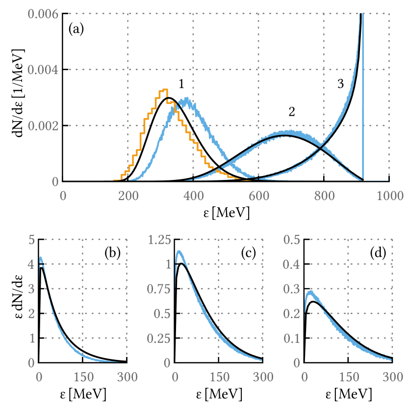
Figure 1: Particle spectra computed with PIC-MC technique (light noisy lines) in the laser pulse — electron beam collision for various pulse duration, and spectra computed in GCFA (black smooth lines), i.e. from Boltzmann’s equations in a constant magnetic field. The magnetic field strength and the interaction time relates with the laser field parameters according to (14)-(15), yielding $\chi=0.1$ in GCFA. Lines 1, 2 and 3 demonstrate the electron spectra, and figures (b), (c) and (d) demonstrate the photon energy spectra for the laser pulse duration of $270$, $68$ and $17\;\mathrm{fs}$, respectively. The orange stepped line 1 in figure (a) shows the result of PIC simulation for a laser pulse with no diffraction. See text for details.

To test GCFA, three dimensional (3D) simulations of the electron beam collision with the laser pulse are performed with PIC code quill [33]. The code quill takes into account photon emission by the Monte Carlo approach similar to rejection sampling [11, 34]. In the simulations the laser pulse longitudinal shape is given by (12), and additional transverse envelope introduced which FWHM along the $y$ and $z$ axes are $y_{s}$ and $z_{s}$, respectively. The duration $x_{L}/c$ and the amplitude of the laser pulse, as well as the initial electron energy $\epsilon_{0}$, are varied to obtain different regimes of the radiation reaction. The interaction time allows complete propagation of all the electrons through the laser pulse. The full electron beam radius ($2\lambda_{L}$) is much smaller than the laser pulse transverse size ($y_{s}=z_{s}=13.4\lambda_{L}$), where $\lambda_{L}=2\pi c/\omega_{L}=1\;\mu\mathrm{m}$ is the laser wavelength.

The results of PIC simulations for unnormalized initial electron energy $\varepsilon_{0}=920\;\mathrm{MeV}$ ($\epsilon=1800$) and $a_{0}=16.5$ are shown in figure 1 with light lines. The maximal quantum parameter reached in this case is $\chi\approx 0.07$. For $x_{L}=82\lambda_{L}\gg 137ct_{rf}$ ($x_{L}/c=270\;\mathrm{fs}$, $137t_{rf}\approx 4.4\;\mathrm{fs}$) FP regime is attained. Accordingly to the central limit theorem, in this case the electron spectrum is close to the Gaussian one [noisy blue line $1$ in figure 1(a)]. The corresponding photon energy spectrum $\epsilon f_{ph}(\epsilon)$ is shown as a light blue line in figure 1(b). Similarly, the electron spectra for $4$ and $16$ times shorter laser pulses ($x_{L}/c=68$ and $17\;\mathrm{fs}$, respectively) are shown as light blue lines $2$ and $3$ in figure 1(a), and the corresponding photon energy spectra are shown in figures 1(c) and (d). Note that for the short laser pulse every electron emits a few photons in the average that makes FP approach [22] and the central limit theorem inapplicable.

The results obtained with Scintillans in GCFA are shown in figure 1 as black lines. Equations (14) and (15) are used to obtain the strength of the constant magnetic field and the interaction time from the parameters of the laser pulses. Thus, black lines $1$, $2$ and $3$ in figure 1(a) are the electron spectra, and in figures 1(b), (c) and (d) are the photon energy distribution $\epsilon f_{ph}(\epsilon)$ for $\mathcal{H}_{0}=250\;\mathrm{kT}$ and $\tau=102$, $26$ and $6.4\;\mathrm{fs}$, respectively. These parameters yield $\mathcal{H}_{0}/E_{S}=5.6\times 10^{-5}$, the initial value of $\chi=0.1$ and the photon emission time $137t_{rf}=3.1\;\mathrm{fs}$.

In Scintillans simulations, as well as in PIC simulation, the electron distribution function is normalised in the same way

$$\int_{0}^{\infty}f_{e}(\epsilon)\,d\epsilon=1.$$ (40)

Note that the parameters of the Scintillans simulation for dark curve $1$ in figure 1(a) are the same as for middle curves in figure 10(c) from Ref. [22], except here initially monoenergetic electron beam with zero temperature is used. Nevertheless, the curve in figure 1(a) is quite close to the corresponding curves from Ref. [22] indicating the consistency between Scintillans and smilei simulations.

For the longest laser pulse an additional PIC simulation is performed in which the laser field is defined analytically in the form (12), with no transverse envelope hence no diffraction. The resulting electron spectrum [orange stepped line 1 in figure 1(a)] is close to that obtained in GCFA, thus the discrepancy between blue and black lines 1 in figure 1(a) is caused by the diffraction. Therefore, it can be concluded from figure 1 that the electron and photon spectra can be described well in GCFA in the classical limit if 1D BE is applicable, even if the number of the emitted photons is small.

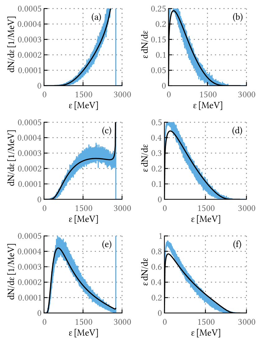
Figure 2: The electron spectrum (left column) and the photon energy spectrum (right column) in laser pulse — electron beam collision computed with PIC-MC technique (light blue lines) and in GCFA (black smooth lines). The laser pulse amplitude varies such that in GCFA initially $\chi=0.3$ for figures (a, b), $\chi=0.6$ for figures (c, d) and $\chi=1.2$ for figures (e, f). See text for details.

Fairly good coincidence between the electron and photon spectra computed in the constant magnetic field and in the laser field forces to test GCFA in the regime of moderate $\chi$ values, $\chi\sim 1$. For this, one should use quite short laser pulses, $x_{L}\lesssim 137t_{rf}$, otherwise the electrons loose almost all initial energy making 1D BE inapplicable. Note that at $\chi\gtrsim 1$ pair photoproduction (which is not taken into account in Scintillans simulations) and subsequent photon emission by secondary electrons and positrons also can spoil BEs. Therefore in the simulations described below $x_{L}/c=17\;\mathrm{fs}$ and $\varepsilon=2.76\;\mathrm{GeV}$ ($\epsilon=5400$) are used. The laser pulse amplitude varies to get different values of $\chi$.

In figure 2 the results of PIC simulations are shown with light blue lines, and the solution of BEs in GCFA obtained with Scintillans are shown with black lines. Figures of the left column demonstrate the electron spectrum $f_{e}(\epsilon)$ whereas the right column is for the photon energy spectrum $\epsilon f_{ph}(\epsilon)$. Figures 2 (a, b), (c, d) and (e, f) correspond to $a_{0}=16.5$, $33$ and $66$, respectively. In GCFA this yields the initial quantum parameter $\chi_{0}=0.3$, $0.6$ and $1.2$. With the increase of the magnetic field strength the photon emission time decreases ($137t_{rf}=3.1$, $1.6$ and $0.8\;\mathrm{fs}$ while $\tau=6.4\;\mathrm{fs}$), the number of photons emitted per electron increases, and the electron distribution tends to lower energies.

From the experimental point of view the mean electron energy

$$\left<\epsilon_{e}\right>=\int_{0}^{\infty}\epsilon f_{e}(\epsilon)\,d\epsilon\times\left[\int_{0}^{\infty}f_{e}(\epsilon)\,d\epsilon\right]^{-1}$$ (41)

and the total energy of gamma photons can characterize the interaction [14, 15]. These quantities are coupled due to energy conservation, and in order to characterize the resulting electron and photon beams one can use instead, for instance, $\left<\varepsilon\right>$, the mean electron energy, and $n_{\gamma}$, the number of photons with energy higher than $100\mathrm{~{}MeV}$, normalized to the number of electrons, which are given in table 1 for all the simulation results depicted in figures 1 and 2. In the table PIC-MC simulation results are noted as ”PIC” and the Scintillans’s results as ”Sc”. The first line of the table includes the results of PIC simulation with laser pulse diffraction incorporated (light blue noisy line 1 in figure 1(a)).

Note that for the parameters of figures 2(a)-(f) almost all assumptions are violated in which equations (14) and (15) are derived. Namely, the emission spectrum is not determined by the classical synchrotron formula and by the critical frequency $\omega_{c}$, e.g. already at $\chi\approx 0.2$ the emission power is only $1/2$ of that computed with the classical formula [10]. Also, the central limit theorem is not valid because the number of the emitted photons is small and the subsequent photon emission events are dependent (the photon energy is of the order of the electron energy). Therefore, a fairly good coincidence between solutions of BEs in GCFA and results of PIC simulations with alternating laser field implies that more reliable basis for the correspondence (14)-(15) can be found.

Table 1: The mean electron energy and the number of photons (per electron) with energy $>100\mathrm{~{}MeV}$ for the simulation results shown in figures 1 and 2.

• figure	$\left<\varepsilon_{e}\right>_{\mathrm{PIC}}\mathrm{[MeV]}$	$\left<\varepsilon_{e}\right>_{\mathrm{Sc}}\mathrm{[MeV]}$	$n_{\gamma,\mathrm{PIC}}$	$n_{\gamma,\mathrm{Sc}}$
  1(a), 1	391	348	0.57	0.83
  1(a), 2	674	667	0.52	0.58
  1(a), 3	845	845	0.18	0.20
  2(a-b)	2347	2335	1.02	0.96
  2(c-d)	1813	1807	2.10	1.91
  2(e-f)	1037	1055	3.66	3.25

5 Conclusion

In this paper we start from the Fokker–Planck (FP) regime of the photon emission when the number of the photons emitted per electron is large and the energy of individual photons is small. For this case two setups are considered: the photon emission by electrons in a constant magnetic field, and the photon emission by electrons in the head-on collision with a laser pulse. The resulting electron spectra are the same in both setups if the setup parameters relate according to (14) and (15). Thus, in FP regime one can compute the electron spectrum in a global constant field approximation (GCFA) instead using alternating laser field. Note that GCFA can be justified also in the supercritical regime $\chi\gg 1$ [35].

PIC simulations demonstrate that the established correspondence (14)-(15) can be used far beyond the FP regime, namely, electron spectrum computed in GCFA fits well the spectrum computed in the laser field for $\chi\approx 1$ (hence the photon energy is comparable with the electron energy) or for small numbers of the emitted photons. Moreover, the spectra of the emitted photons in the constant magnetic field and in the laser field coincides fairly well with each other in these cases.

In GCFA the electron and photon spectra can be efficiently computed from 1D Boltzmann’s equations, for what the Scintillans open source code is developed [31]. The code conserves exactly the number of electrons and the total particle energy. Obviously, in 1D Boltzmann’s equations neither pulse diffraction nor collective effects in the electron beam [15] are taken into account. However, the mentioned effects are generally small and can be neglected for typical parameters of laser pulse — electron beam interactions.

Theoretical analysis of radiation reaction in laser fields, e.g. analysis of the stochasticity effect, is a quite complicated task and often requires numerical simulations [36, 22, 26, 21]. Radiation reaction in a constant magnetic field looks much more simple than in the alternating field, thus GCFA opens perspectives of fully theoretical advance of the topic.

In the context of recent experimental study of radiation reaction [14, 15], GCFA can be useful as well. Scintillans simulations takes time of seconds opposite to PIC simulations that takes at least minutes, hence a search of optimal experimental parameters [37] can be easier in GCFA. Furthermore, in the experiments with electron spectrum known before and after the collision [15], one can find the laser pulse amplitude and duration from a comparison of the experimental results with results of Scintillans simulations in a large region of parameters. Such comparison probably will allow to evade experimental uncertainties and to distinguish clearly different radiation reaction models.

References

- [1] Weller H R, Ahmed M W, Gao H, Tornow W, Wu Y K, Gai M and Miskimen R 2009 Progress in Particle and Nuclear Physics, Volume 62, Issue 1, p. 257-303. 62 257–303
- [2] High intensity gamma-ray source (higs) URL http://www.tunl.duke.edu/facilities/
- [3] Ando A, Amano S, Hashimoto S, Kinosita H, Miyamoto S, Mochizuki T, Niibe M, Shoji Y, Terasawa M, Watanabe T and Kumagai K 1998 J. Synchrotron Rad. 5 342–344
- [4] Newsubaru synchrotron radiation facility URL http://www.lasti.u-hyogo.ac.jp/NS-en/facility/
- [5] Adriani O, Albergo S, Alesini D, Anania M, Angal-Kalinin D, Antici P, Bacci A, Bedogni R, Bellaveglia M, Biscari C et al. 2014 arXiv preprint arXiv:1407.3669
- [6] Extreme light infrastructure - nuclear physics (eli-np) URL http://www.eli-np.ro/
- [7] Balabanski D L 2018 Journal of Physics: Conference Series 966 012018 URL http://stacks.iop.org/1742-6596/966/i=1/a=012018
- [8] Sarri G, Corvan D J, Schumaker W, Cole J M, Di Piazza A, Ahmed H, Harvey C, Keitel C H, Krushelnick K, Mangles S P D, Najmudin Z, Symes D, Thomas A G R, Yeung M, Zhao Z and Zepf M 2014 Physical Review Letters 113 224801
- [9] Yan W, Fruhling C, Golovin G, Haden D, Luo J, Zhang P, Zhao B, Zhang J, Liu C, Chen M, Chen S, Banerjee S and Umstadter D 2017 Nature Photonics 11 514
- [10] Berestetskii V B, Lifshitz E M and Pitaevskii L P 1982 Quantum Electrodynamics (New York: Pergamon)
- [11] Elkina N V, Fedotov A M, Kostyukov I Y, Legkov M V, Narozhny N B, Nerush E N and Ruhl H 2011 Physical Review Special Topics - Accelerators and Beams 14 054401
- [12] Burke D L, Field R C, Horton-Smith G, Spencer J E, Walz D, Berridge S C, Bugg W M, Shmakov K, Weidemann A W, Bula C, McDonald K T, Prebys E J, Bamber C, Boege S J, Koffas T, Kotseroglou T, Melissinos A C, Meyerhofer D D, Reis D A and Ragg W 1997 Phys. Rev. Lett. 79 1626–1629
- [13] Bamber C, Boege S J, Koffas T, Kotseroglou T, Melissinos A C, Meyerhofer D D, Reis D A, Ragg W, Bula C, McDonald K T, Prebys E J, Burke D L, Field R C, Horton-Smith G, Spencer J E, Walz D, Berridge S C, Bugg W M, Shmakov K and Weidemann A W 1999 Phys. Rev. D 60 092004
- [14] Cole J M, Behm K T, Gerstmayr E, Blackburn T G, Wood J C, Baird C D, Duff M J, Harvey C, Ilderton A, Joglekar A S, Krushelnick K, Kuschel S, Marklund M, McKenna P, Murphy C D, Poder K, Ridgers C P, Samarin G M, Sarri G, Symes D R, Thomas A G R, Warwick J, Zepf M, Najmudin Z and Mangles S P D 2018 Physical Review X 8 011020
- [15] Poder K, Tamburini M, Sarri G, Di Piazza A, Kuschel S, Baird C D, Behm K, Bohlen S, Cole J M, Corvan D J, Duff M, Gerstmayr E, Keitel C H, Krushelnick K, Mangles S P D, McKenna P, Murphy C D, Najmudin Z, Ridgers C P, Samarin G M, Symes D R, Thomas A G R, Warwick J and Zepf M 2018 Phys. Rev. X 8 031004 URL https://link.aps.org/doi/10.1103/PhysRevE.97.043209
- [16] Wistisen T N, Di Piazza A, Knudsen H V and Uggerhøj U I 2018 Nature Communications 9 795
- [17] Macchi A 2018 Physics 11 13
- [18] Di Piazza A, Tamburini M, Meuren S and Keitel C H 2019 Phys. Rev. A 99 022125 URL https://link.aps.org/doi/10.1103/PhysRevA.99.022125
- [19] Nerush E N and Kostyukov I Y 2011 Nuclear Instruments and Methods in Physics Research A 653 7–10
- [20] Ridgers C P, Kirk J G, Duclous R, Blackburn T G, Brady C S, Bennett K, Arber T D and Bell A R 2014 Journal of Computational Physics 260 273–285 ISSN 0021-9991 URL http://www.sciencedirect.com/science/article/pii/S0021999113008061
- [21] Vranic M, Grismayer T, Fonseca R A and Silva L O 2016 New Journal of Physics 18 073035 URL http://stacks.iop.org/1367-2630/18/i=7/a=073035
- [22] Niel F, Riconda C, Amiranoff F, Duclous R and Grech M 2018 Phys. Rev. E 97 043209 URL https://link.aps.org/doi/10.1103/PhysRevE.97.043209
- [23] Nerush E N, Bashmakov V F and Kostyukov I Y 2011 Physics of Plasmas 18 083107
- [24] Bulanov S S, Schroeder C B, Esarey E and Leemans W P 2013 Physical Review A 87 62110
- [25] Kirillov A A 2008 An introduction to Lie groups and Lie algebras vol 113 (Cambridge University Press)
- [26] Niel F, Riconda C, Amiranoff F, Lobet M, Derouillat J, Pérez F, Vinci T and Grech M 2018 Plasma Physics and Controlled Fusion 60 094002 URL http://stacks.iop.org/0741-3335/60/i=9/a=094002
- [27] Baier V N and Katkov V M 1967 Physics Letters A, Volume 25, Issue 7, p. 492-493. 25 492–493
- [28] Baier V N, Katkov V and Strakhovenko V 1998 Electromagnetic processes at high energies in oriented single crystals (Singapore: World Scientific)
- [29] Landau L D and Lifshitz E M 1975 (Oxford: Elsevier)
- [30] Bashinov A V, Kim A V and Sergeev A M 2015 Physical Review E 92 043105
- [31] Tool to solve 1d boltzmann’s equations for electrons emitting photons URL https://github.com/EvgenyNerush/scintillans
- [32] Lippmeier B, Chakravarty M, Keller G and Peyton Jones S 2013 ACM SIGPLAN Notices 47 25–36
- [33] Three-dimensional parallel particle-in-cell code quill for investigation of electron-positron cascades development URL http://iapras.ru/english/structure/dep_330/quill.html
- [34] Nerush E N, Serebryakov D A and Kostyukov I Y 2017 The Astrophysical Journal 851 129
- [35] Baumann C, Nerush E N, Pukhov A and Kostyukov I Y 2018 arXiv preprint arXiv:1811.03990
- [36] Duclous R, Kirk J G and Bell A R 2011 Plasma Physics and Controlled Fusion 53 015009
- [37] Arran C, Cole J M, Gerstmayr E, Blackburn T G, Mangles S P D and Ridgers C P 2019 arxiv preprint arXiv:1901.09015