Zoom-in cosmological hydrodynamical simulation of a star-forming barred, spiral galaxy at redshift $z=2$

Abstract

We present gas and stellar kinematics of a high-resolution zoom-in cosmological chemodynamical simulation, which fortuitously captures the formation and evolution of a star-forming barred spiral galaxy, from redshift $z\sim 3$ to $z\sim 2$ at the peak of the cosmic star formation rate. The galaxy disc grows by accreting gas and substructures from the environment. The spiral pattern becomes fully organised when the gas settles from a thick (with vertical dispersion $\sigma_{v}>$ 50 km/s) to a thin ($\sigma_{v}\sim 25$ km/s) disc component in less than 1 Gyr. Our simulated disc galaxy also has a central X-shaped bar, the seed of which formed by the assembly of dense gas-rich clumps by $z\sim 3$. The star formation activity in the galaxy mainly happens in the bulge and in several clumps along the spiral arms at all redshifts, with the clumps increasing in number and size as the simulation approaches $z=2$. We find that stellar populations with decreasing age are concentrated towards lower galactic latitudes, being more supported by rotation, and having also lower velocity dispersion; furthermore, the stellar populations on the thin disc are the youngest and have the highest average metallicities. The pattern of the spiral arms rotates like a solid body with a constant angular velocity as a function of radius, which is much lower than the angular velocity of the stars and gas on the thin disc; moreover, the angular velocity of the spiral arms steadily increases as function of time, always keeping its radial profile constant. The origin of our spiral arms is also discussed.

1 Introduction

The formation and evolution of the basic properties of galaxies can be roughly explained in a cosmological context, with the growth followed by the hierarchical clustering of dark matter (DM) halos and feedback from stars and active galactic nuclei (AGNs). However, the formation and evolution of the detailed internal structural properties of galaxies have not been well explained yet (Conselice, 2014; Dobbs & Baba, 2014). The origin of the Hubble sequence (Hubble, 1926) remains a theoretical challenge (Benson, 2010; Cen, 2014; Genel et al., 2015; Clauwens et al., 2018). Spiral galaxies are one of the most popular Hubble morphological types in the local Universe. (e.g., Willett et al. 2013). The essential components of spiral galaxies include spiral arms, bars, bulges, thin and thick discs.

The spatially-resolved properties of stellar populations in nearby spiral galaxies are obtained with UV, optical, and infrared observations (Rix & Rieke, 1993; Thornley, 1996; Davis et al., 2017; Sánchez-Menguiano et al., 2017; Yu et al., 2018), while the physical properties of the gas can be investigated in detail by means of high-resolution interferometry (e.g. Walter et al. 2008; Schinnerer et al. 2013; Tacconi et al. 2013; Koribalski et al. 2018); to this end, the first observational cycles of the Atacama Large Millimeter Array (ALMA) are providing data of unprecedented quality, probing different phases of the interstellar medium (ISM) by making use of the spatial and velocity distributions of different molecular species in the galaxy (e.g., Faesi et al. 2018; Sun et al. 2018; Wilson 2018).

Observations can now resolve internal structures like spiral arms at high redshift ($z=2-3$), an epoch when the Hubble sequence is speculated to emerge (Law et al., 2012; Conselice, 2014; Yuan et al., 2017). The highest spatial resolution observations at high redshift are usually achieved in small numbers by the technique of gravitational lensing and adaptive-optics aided integral field spectroscopy (IFS). With high accuracy gravitational lensing models, high-redshift galaxies can be resolved on $\sim$100 pc scales (e.g., Sharma et al. 2018). Thanks to ALMA and, in the future, the Square Kilometer Array (SKA), we are reaching the sensitivity and resolution power to probe star-forming disc galaxies at even higher redshifts of $z\gtrsim 3$ (e.g., Hodge et al. 2018). With $\sim$ kpc resolutions, large IFS surveys such as CALIFA (Sánchez et al., 2016), MaNGA (Bundy et al., 2015) and SAMI (Croom et al., 2012) can provide local baselines of dynamical mapping of thousands of late-type galaxies. Seeing-limited SINFONI (Bonnet et al., 2004; Förster Schreiber et al., 2009) and KMOS (Stott et al., 2016) surveys provide similar information on a few kpc scales for large numbers of galaxies at $z\sim 1-2$. In the near future, NIRSpec/JWST (Posselt et al., 2004; Alves de Oliveira et al., 2018) will provide sub-kpc scale observations on rest-frame UV and optical properties of large samples of galaxies at $z\gtrsim 2$. High-resolution cosmological simulations will therefore need to be ready to predict and explain the evolution of galaxy structures at high redshift.

In the past, several works investigated the formation and evolution of star-forming disc galaxies with cosmological simulation techniques, starting – for example – from the very early numerical attempts that did not form realistic discs yet (Katz & Gunn, 1991; Navarro & Steinmetz, 2000; Abadi et al., 2003), to more recent efforts that successfully developed disc-dominated systems (e.g., Scannapieco et al. 2008; Agertz, Teyssier & Moore 2009, 2011; Guedes et al. 2011; Aumer et al. 2013; Stinson et al. 2013; Hopkins, Kereš & Murray 2013; Marinacci, Pakmor & Springel 2014; Übler et al. 2014; Grand, et al. 2015; Colín et al. 2016). Finally, Grand, et al. (2017) showed that cosmological zoom-in simulations can be used to investigate spiral arms and infer their nature at $z\sim 0$.

The Hubble classification defines spiral galaxies with or without bars. The physical processes driving the formation and the growth of such structures, as well as those maintaining the stability of the gaseous and the stellar disc of galaxies against the pulling forces from both the environment and the feedback from the star formation activity, are still a matter of debate in the astronomical community (Dobbs & Baba, 2014; Davis et al., 2015; Schinnerer et al., 2017). In summary, the main theories for the origin of spiral arms in disc galaxies are the density wave theory (Lindblad, 1960; Lin & Shu, 1964, 1966; Kalnajs, 1971); the swing amplification mechanism (e.g., Goldreich & Lynden-Bell 1965; Julian & Toomre 1966; Toomre 1981; Masset & Tagger 1997; D’Onghia, Vogelsberger & Hernquist 2013), the multiple mode theory (e.g., Quillen et al. 2011; Comparetta & Quillen 2012; Sellwood & Carlberg 2014); the manifold theory (e.g., Athanassoula 2012; Efthymiopoulos, Kyziropoulos, Páez, Zouloumi & Gravvanis 2019), and the theory of corotating or dynamical spiral arms (e.g., Wada, Baba & Saitoh 2011; Grand, Kawata & Cropper 2012; Baba, Saitoh & Wada 2013). Bars and tidal interactions can also drive spiral density waves on a galatic scale (Kormendy & Norman, 1979; Salo & Laurikainen, 1993; Dobbs et al., 2010), giving rise to the so-called kinematic density waves (see also Kalnajs 1973; Oh, Kim, Lee & Kim 2008; Struck, Dobbs & Hwang 2011; Oh, Kim & Lee 2015). Finally, another proposed viable mechanism to develop spiral arms is through the accretion of substructures and gas from the environment into the galaxy gravitational potential (Sellwood & Carlberg, 1984). We remark on the fact that almost all simulations have so far found spiral arms as being a transient phenomenon, occurring over a large range of timescales, typically from $\sim 1\,\text{Gyr}$ to $\sim 10\,\text{Gyr}$ (Sellwood & Binney, 2002; Fujii et al., 2011).

The different theories for the formation of spiral arms predict different characteristic evolution of the dynamical properties of the gas and stars on the spiral arms as functions of time. For example, manifold-driven spiral arms have been proven to create an angular velocity pattern which appears as constant as a function of time, because – by assuming a bar co-rotating reference frame – the trajectories of the particles on the spiral arms are confined in the spiral arms themselves, which line up with the unstable Lagrange points of the bar (the invariant manifolds) (Athanassoula, 2012); on the other hand, the kinematic density-wave theory – an other largely favourite theory, giving also rise to a constant angular speed of the spiral arm perturbation as a function of radius – predict the density waves to show up in the Fourier power spectrum as a power along the inner Lindblad resonance (Kalnajs, 1973). Nevertheless, it is not straightforward to compare these theoretical predictions to observations. In the Milky Way, it is possible to measure the ages of individual stars, from which it is possible to derive the dynamical evolution (e.g., Rix & Bovy 2013; Bland-Hawthorn & Gerhard 2016), but for external galaxies, observations provide an instantaneous snapshot of the properties of the stellar populations and gas in the galaxy disc.

Even if we wanted to compare the spatial distribution and the kinematics of stars with different ages lying in the observed galaxy disc, to determine the best scenario for the formation of the spiral arms, the observed integrated spectrum from a given galaxy region is contributed by a mixture of stars with different ages and metallicities. This can be disentangled only by making use of stellar population synthesis models, which – in turn – strongly depend on the assumed initial mass function (IMF), star formation history (SFH), stellar evolutionary tracks, and library of stellar spectra. Therefore, the final observational results may strongly depend on the assumptions of models. For this reason, direct comparisons of observed stellar populations with those predicted from spiral arm formation theories are only available very recently with IFS data of nearby galaxies (e.g., Peterken et al. 2018).

The significant decrease in the observed volume density of spiral galaxies at high redshift implies a close connection between the formation of spiral arms and thin discs (Yuan et al., 2017). Most spiral arms in the local Universe reside in a rotating thin disc (vertical height of 200-300 pc) of high angular momentum (Epinat et al., 2008; Glazebrook, 2013). Studies of the Milky Way show that the thin disc of our Galaxy formed around $z\sim 0.8-1$ (Freeman, & Bland-Hawthorn, 2002; Haywood et al., 2016). However, whether other spiral galaxies follow the same formation history as the Milky Way is unknown. The question of whether the thin disc formed before or after the thick disc is also contentious (Freeman, & Bland-Hawthorn, 2002; Rix & Bovy, 2013). Forming a large rotating disc at $z>1$ is theoretically difficult because it takes considerable time to accumulate angular momentum from the accreted halo gas (Catelan, & Theuns, 1996; Lagos et al., 2017). Due to limited resolutions, the formation and evolution of large thin discs with cosmic time and and their relation to spiral arms are thus far rarely explored in cosmological simulations.

In this paper, we present the first high-resolution chemodynamical zoom-in simulation for the formation of a star-forming barred spiral galaxy at high redshift ($z\geq 2$), within a full cosmological framework. This allows us to study a disc galaxy that forms and evolves though a large-scale gas accretion, as well as undergoes star formation, feedback, and chemical enrichment within the galaxy. We characterise in detail the evolution of the physical and kinematical properties of the gas and stellar populations during the formation of the bar and spiral structures in the galaxy.

This paper is structured as follows. In Section 2, we introduce the basic assumptions of our simulation code, presenting both the parent large-volume cosmological simulation and the zoom-in simulation. In Section 3, we present the results of our paper. Finally, in Section 5, we draw our conclusions.

2 Simulation model and methods

2.1 The simulation code

We make use of our chemodynamical code (Kobayashi et al., 2007; Vincenzo & Kobayashi, 2018b), based on Gadget-3 (Springel, 2005), which adopts the smoothed particle hydrodynamics (SPH) method to solve the equations of motion of the fluid elements, together with their thermodynamical properties (Monaghan, 1992).

Our model takes into account three distinct kinds of particles; we have (i) gas particles, (ii) star particles, and (iii) dark matter (DM) particles. All these three kinds of particles interact with each other via their mutual gravitational interaction, and only the physical attributes of gas particles are computed by means of the SPH solver. For instance, the main physical attributes of gas particles are their position, velocity, mass, density, temperature, pressure, electron density, smoothing length, SFR, and chemical abundances, while the main physical attributes of star particles are their position, velocity, mass, initial mass, formation time, and chemical abundances.

Our scientific target is a young disc galaxy; we do not consider any black hole physics and associated feedback from AGNs. We address the readers to the work of Taylor & Kobayashi (2014, and subsequent papers of the same authors) for more details about how black hole physics and AGN feedback have been included in our simulation code, to reproduce the observational properties of early-type galaxies and AGN-host galaxies as functions of redshift.

Figure 1: In this figure, we show our simulated star-forming disc galaxy within its closest surrounding environment at redshift $z=2$. In the top panel, the galaxy is rotated to be viewed edge-on, while in the bottom panel it is face-on. The colour coding corresponds to the gas density, in logarithmic units, normalised to the maximum gas density within the considered region.

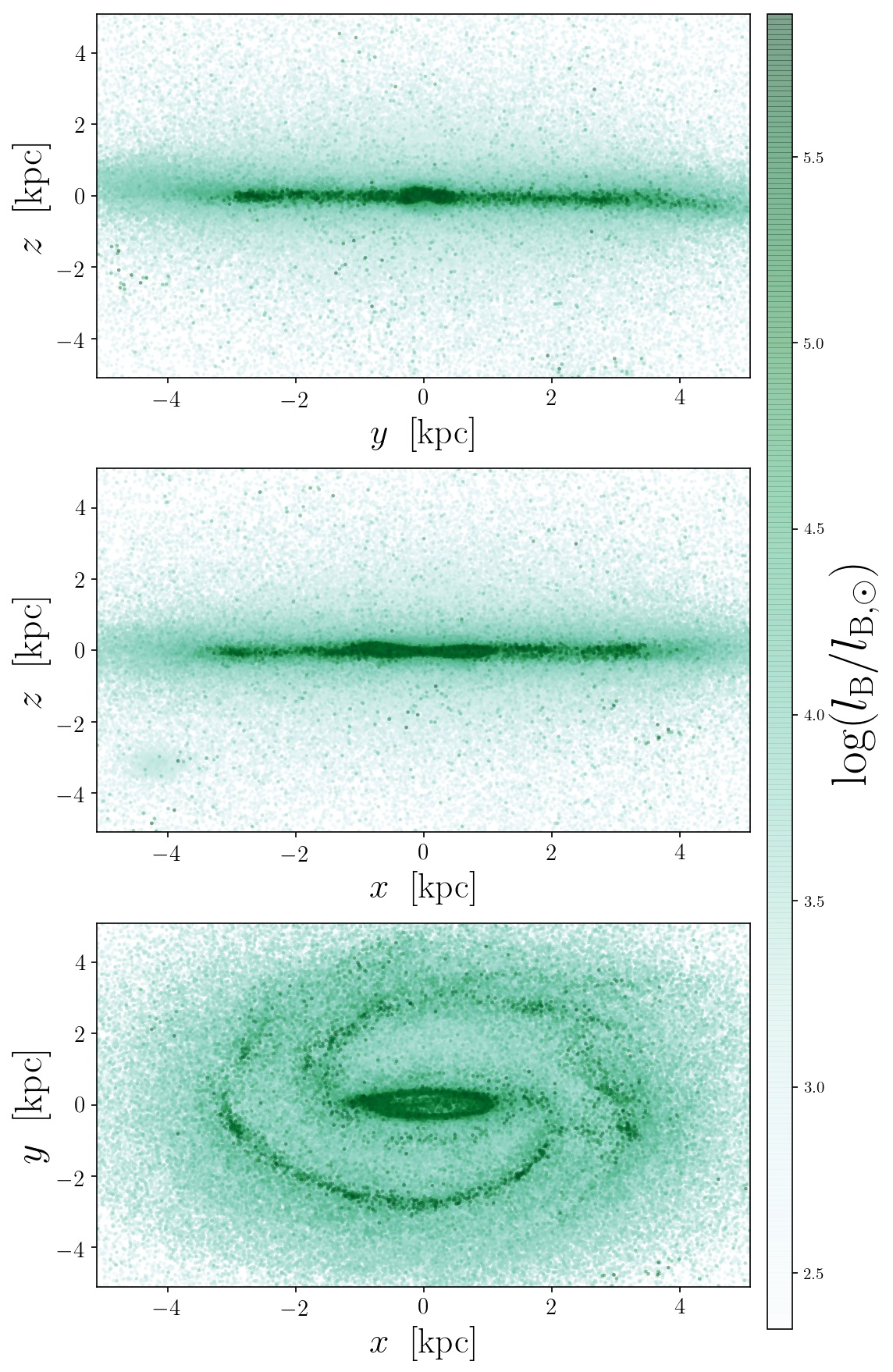
Figure 2: In this figure, we show how our simulated star-forming barred disc galaxy looks like at redshift $z=2$ when its stellar populations are lighted up in the B-band, by using the photometric population synthesis model of Vincenzo et al. (2016); in particular, this figure contains $845,083$ star particles, which are drawn in the order of their B-band luminosity, $l_{\text{B}}$ , which represents also the colour coding (in logarithmic units, normalised to the solar B-band luminosity).

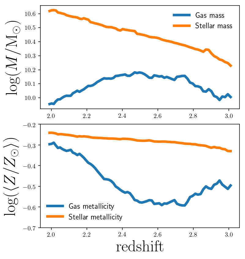
Figure 3: The top panel shows the evolution of the total galaxy stellar and gas mass as functions of redshift. The bottom panel shows the redshift evolution of the average stellar and gas-phase metallicities, in logarithmic units, normalised with respect to the solar metallicity, $Z_{\sun}=0.0134$ by Asplund et al. (2009).

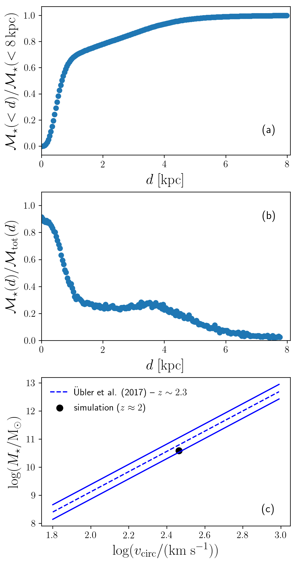
Figure 4: (a) Cumulative galaxy stellar mass as a function of the galactocentric distance. (b) Radial profile of the stellar-to-total mass ratio, where $\mathcal{M}_{\text{tot}}$ includes the DM, star, and gas components. (c) Observed average Tully-Fisher relation at redshift $z\sim 2.3$ from Übler, et al. (2017) is shown as the blue dashed line with the $\pm 1\sigma$ deviations as blue solid lines, as compared with the predicted values at $z\approx 2$ in our simulated disc galaxy.

2.1.1 Chemical enrichment

Our simulation code includes the most detailed chemical enrichment routine, compared with other hydrodynamical codes. All major stellar nucleosynthetic sources are included, namely core-collapse (Type II and hypernovae, HNe) and Type Ia supernovae (SNe), asymptotic giant branch stars (AGBs), and stellar winds from stars of all masses and metallicities. We remark on the fact that the chemical abundances associated to a given star particle, $\mathcal{S}_{i}$, correspond to those of the gas particle, $\mathcal{G}_{j}$, at the time $\mathcal{S}_{i}$ originated in the past.

The feedback from the star formation activity depends on both the metallicity and age of the star particles. For the stellar yields and thermal energy feedback, we follow the same prescriptions as in Kobayashi et al. (2007), but updated to include failed SNe (Vincenzo & Kobayashi, 2018a, b). For Type Ia SNe, we assume the single-degenerate scenario with metallicity-dependent white dwarfs winds (Kobayashi & Nomoto, 2009). Moreover, we assume that the nucleosynthetic products and the thermal energy feedback from the ageing star particles in the simulation box are distributed to $N_{\mathrm{FB}}=288$ of neighbour gas particles, weighted by the smoothing kernel. Finally, the mass spectrum of the stars within each star particle defines the so-called initial mass function (IMF), which – in our model – follows the distribution of Kroupa (2008), very similar to Chabrier (2003).

2.2 The zoom-in simulation

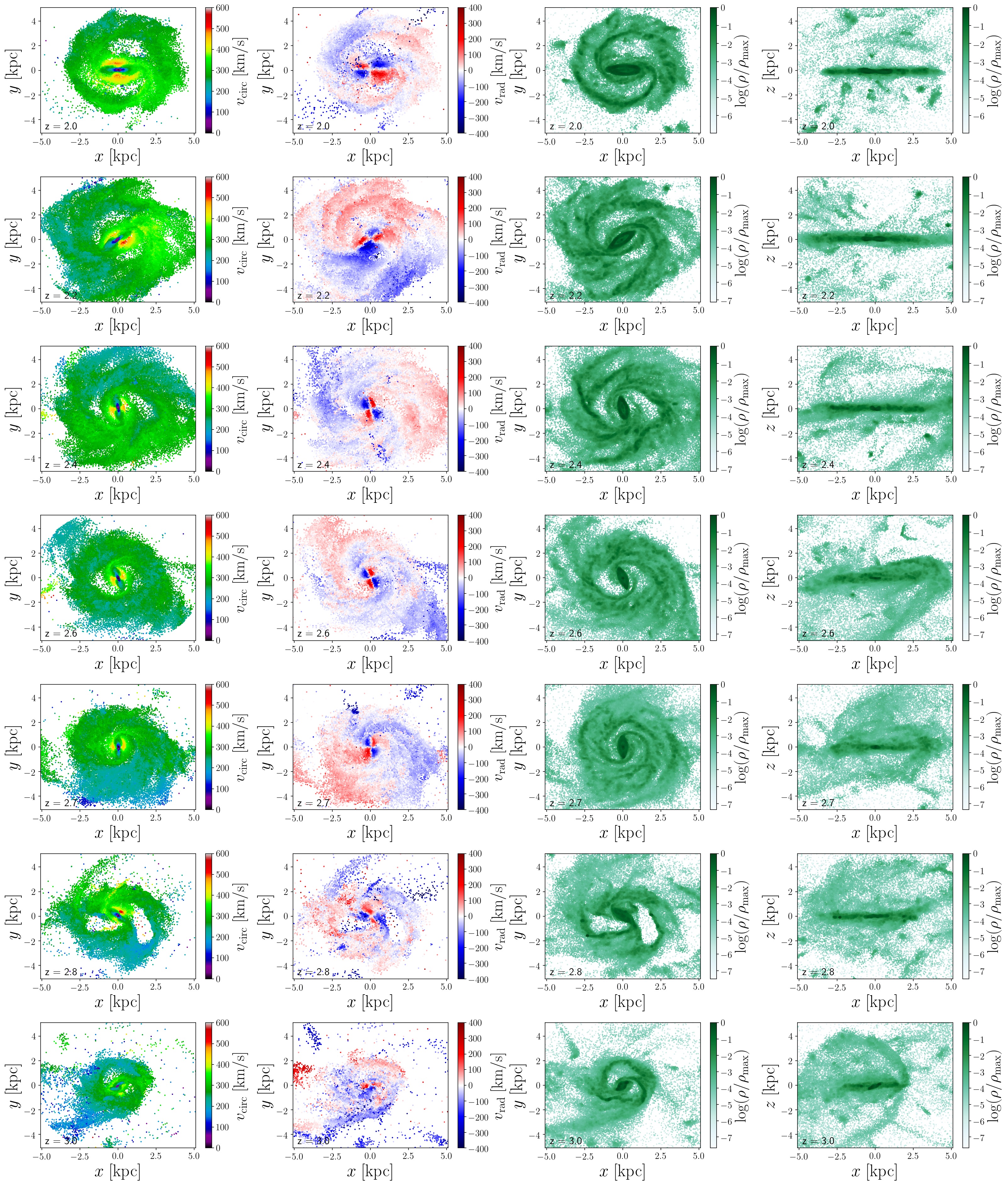
Figure 5: The velocity and density fields within our simulated galaxy as functions of redshift, from $z=3$ to $z=2$ (from the bottom to the top panels). In particular, from left to right, the various columns show similar maps of the simulated galaxy at a given redshift, where the colour coding is given by (i) the circular velocity of the gas particles (where galaxy is seen face-on), (ii) the radial velocity of the gas particles (where galaxy is seen face-on), (iii) the gas density (where galaxy is seen face-on), and (iv) the gas density (where galaxy is seen edge-on).

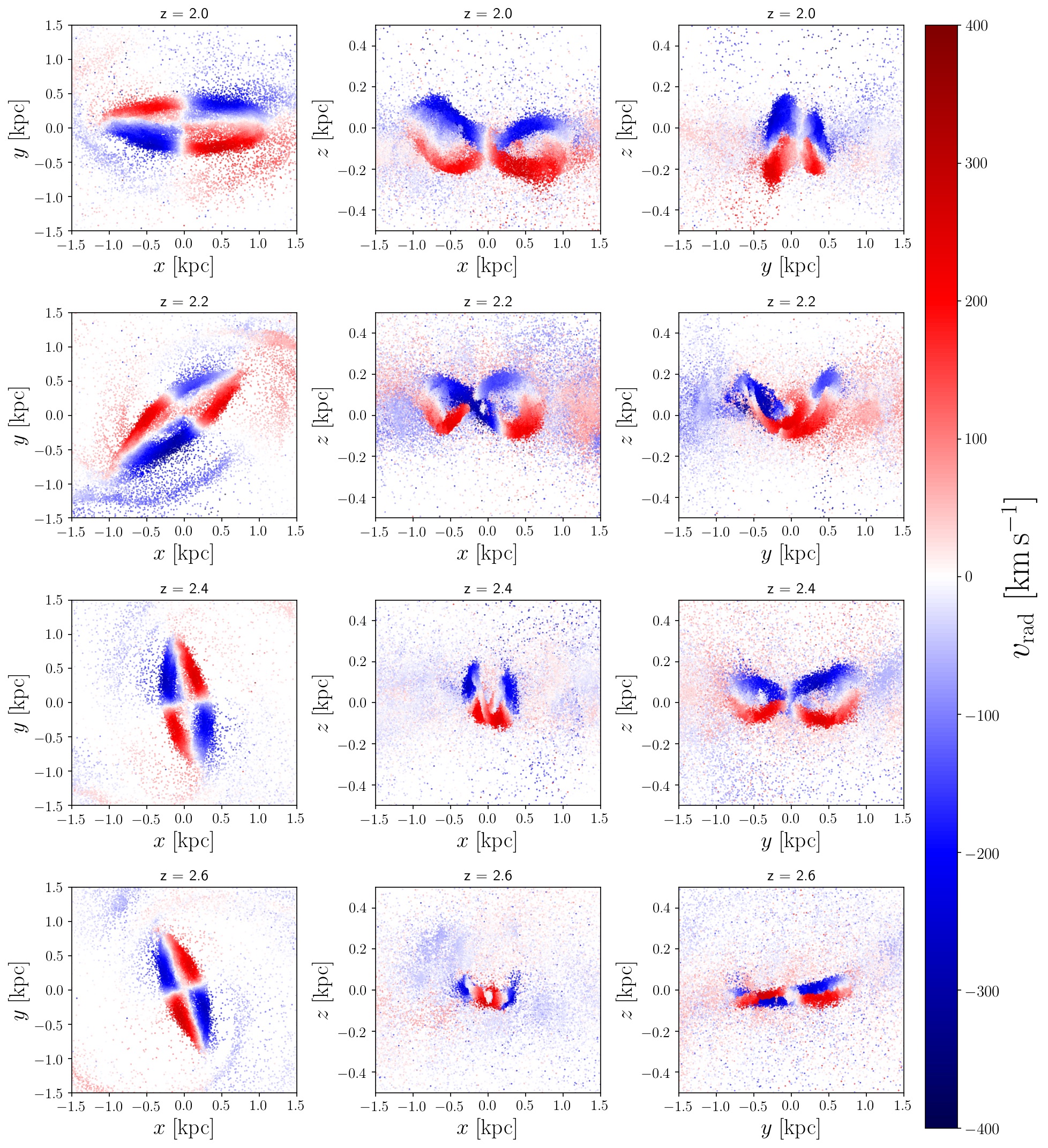
Figure 6: The galaxy bar seen face-on in the $x$-$y$ plane (first column), edge-on in the $x$-$z$ plane (second column), and edge-on in the $y$-$z$ plane (third column). From bottom to top, each row of panels shows the galactic bar at a given redshift, with the colour coding representing the radial component of the velocity field of the gas particles.

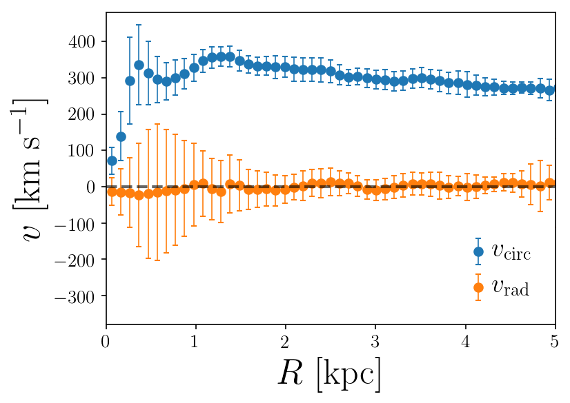
Figure 7: The radial profiles of the circular (blue points) and radial (orange points) velocity patterns of the gas particles in our simulated galaxy as functions of the galactocentric distance at $z=2$.

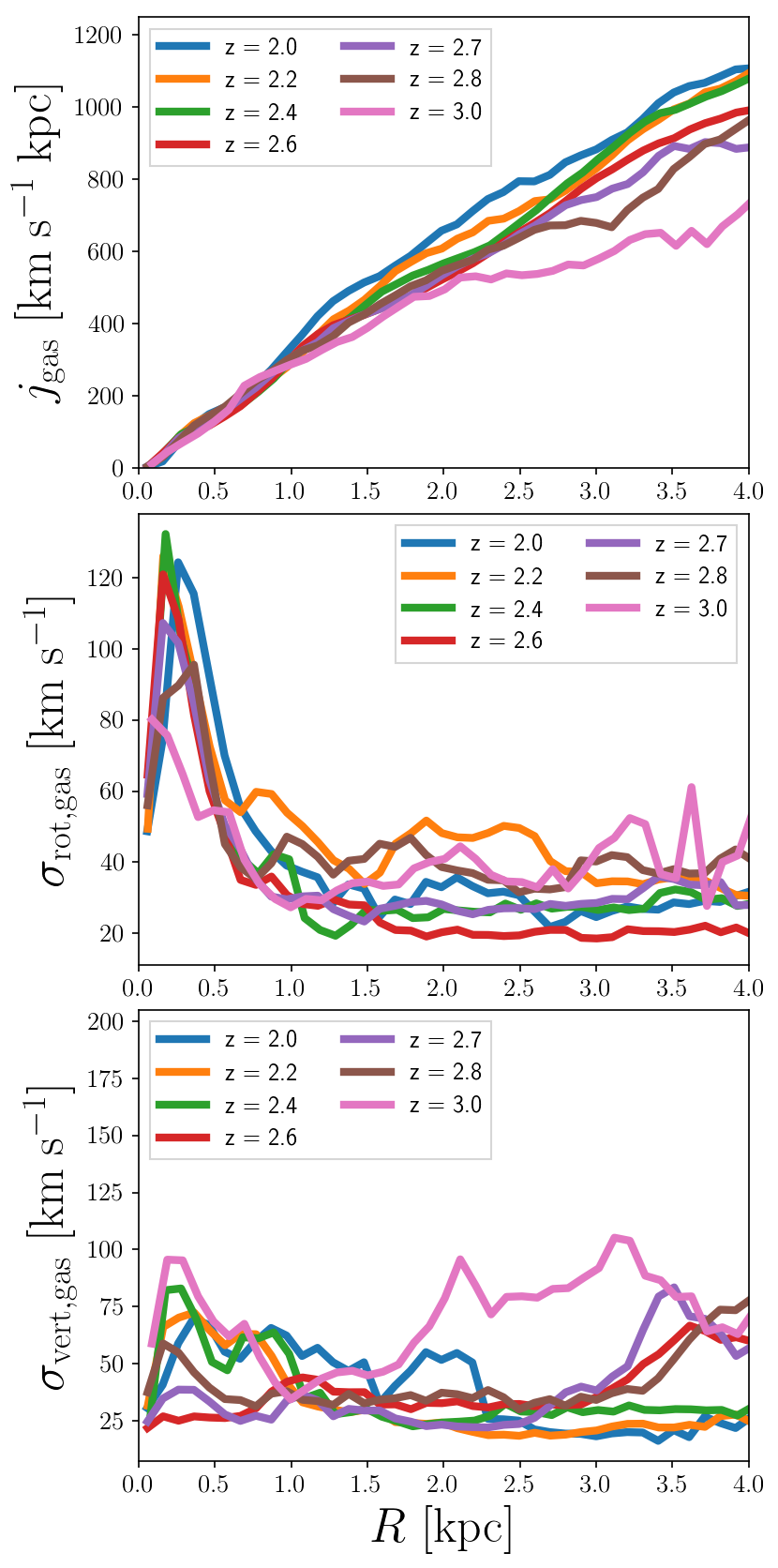
Figure 8: From top to bottom, the various panels show the redshift evolution of the radial profiles of the specific angular momentum, rotational velocity dispersion, and vertical velocity dispersion of the gas particles in our simulated galaxy.

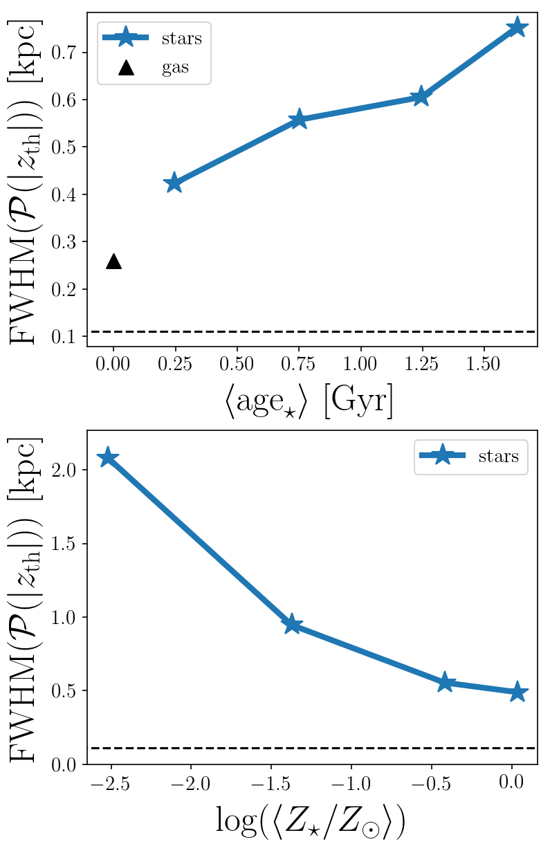
Figure 9: In the top panel, we show how the full width at half maximum (FWHM) of the height distribution of the galaxy stellar populations, $\mathcal{P}(\lvert z_{\text{th}}\rvert)$, varies as a function of the average stellar age at $z=2$; the black triangle corresponds to the FWHM of the height distribution of the galaxy gas particles, which are predicted to lie on a thin disc at $z=2$. The bottom panel shows the FWHM of the height distribution of the galaxy stellar populations as a function of the average stellar metallicity. The dashed horizontal line in both panels represents the softening length of our simulation at redshift $z=2$ in physical units ($\epsilon_{\mathrm{gas}}\approx 0.11\;\mathrm{kpc}$).

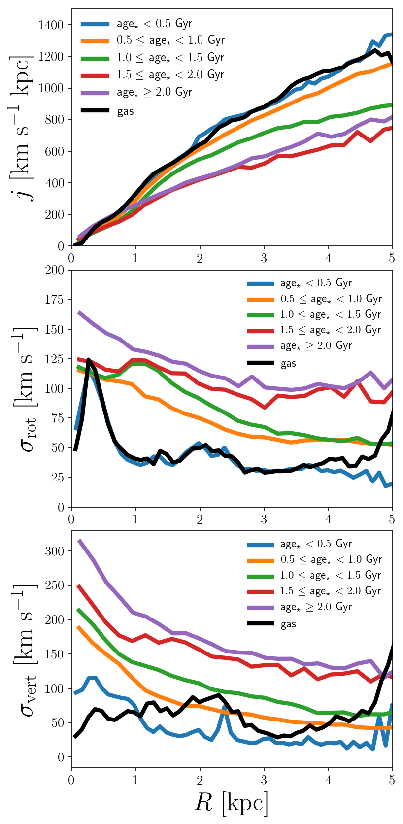
Figure 10: From top to bottom, each panel corresponds to the predicted radial profiles at redshift $z=2$ of the following quantities: (i) specific angular momentum, (ii) rotational velocity dispersion, and (iii) vertical velocity dispersion. The various curves in each panel correspond to stellar populations in different age bins, with the black curve corresponding to the gas particles.

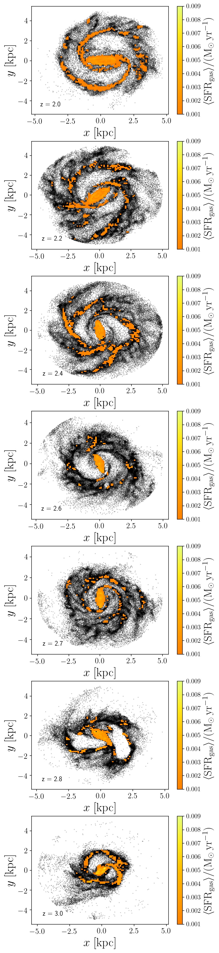
Figure 11: From bottom to top, the redshift evolution from $z=3$ down to $z=2$ of the SFR map within our simulated galaxy, viewed face-on. The black points in the background represent all the gas particles on the disc of our simulated galaxy, while the yellow points highlight the gas particles which are star-forming at the given redshift.

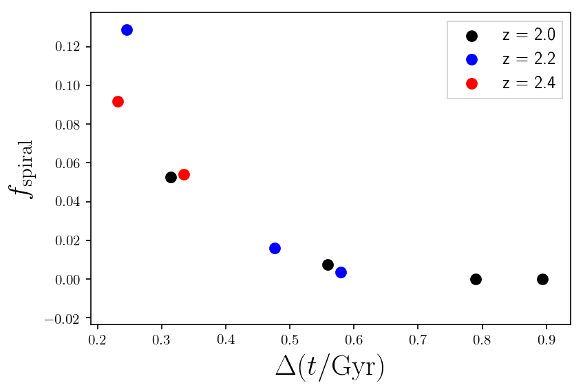
Figure 12: The fraction of star particles, $f_{\text{spiral}}$, which reside on the spiral arms both at redshift $z$ (which represents the colour coding of the figure) and at previous epochs of the galaxy evolution $z^{\prime}=z-\Delta z$. In particular, we compute $f_{\text{spiral}}(z)$ for different values of $z^{\prime}$ in the past, which are then translated into values of look-back time. For example, if we compare the stellar populations on the spiral arms at redshift $z=2$ with those on the spiral arms at a time $0.3\,\text{Gyr}$ before $z=2$, we find that they only have $\sim 5$ per cent of stellar populations on the arms in common.

The starting point of this work is represented by a parent cosmological hydrodynamical simulation of a cubic volume of the Universe, with comoving side $10\,\mathrm{Mpc}\,h^{-1}$, and periodic boundary conditions, from which the zoom-in simulation is later set up.

The parent cosmological simulation — The initial conditions of the parent simulation are drawn by using the MUSIC code (Hahn & Abel, 2011). We assume the standard $\Lambda$-cold DM cosmological model, with the following parameters: $\Omega_{0}=0.31$, $\Omega_{\Lambda}=0.69$, $\Omega_{\mathrm{b}}=0.048$, $h=H_{0}/(100\,\text{km}\,\text{s}^{-1}\,\text{Mpc}^{-1})=0.68$, and $\sigma_{8}=0.82$, as given by Planck Collaboration et al. (2016, 2018). In the parent simulation, we assume a total number of DM and gas particles $N_{\mathrm{DM}}=N_{\mathrm{gas}}=128^{3}$, which leads to the following mass resolutions in the initial conditions: $M_{\mathrm{DM}}\approx 3.47\times 10^{7}\,h^{-1}\,\mathrm{M}_{\sun}$ for the DM particles, and $M_{\mathrm{gas}}=6.35\times 10^{6}\,h^{-1}\,\mathrm{M}_{\sun}$ for the gas particles. The gravitational softnening length is set as $\epsilon_{\mathrm{gas}}\approx 0.84\,h^{-1}\;\mathrm{kpc}$ in comoving units.

The target DM halo — In summary, a target DM halo is selected in the parent cosmological simulation at redshift $z=0$, and then re-simulated from the initial conditions (at redshift $z=49$) with a much larger number of particles, giving rise to a zoom-in cosmological simulation. Our target DM halo in the parent simulation is selected, because it is fairly isolated, it has few substructures, and it lies within a less dense environment than the other DM halos in the simulated cosmological volume. By considering the mass within the virial radius, which is $r_{\text{vir}}\approx 259\,\text{kpc}/h$, the target DM halo in the parent simulation has, at redshift $z=0$, a total mass $M_{\text{DM,h}}=3.35\times 10^{12}\,h^{-1}\,\mathrm{M}_{\sun}$ in the DM component, total stellar mass $M_{\star,\text{h}}=1.78\times 10^{11}\,h^{-1}\,\mathrm{M}_{\sun}$, and total gas mass $M_{\text{gas,h}}=3.76\times 10^{11}\,h^{-1}\,\mathrm{M}_{\sun}$. By looking at the central galaxy in the target DM halo of our parent cosmological simulation at redshift $z=0$, its SFH in the last $3$ Gyr has been steadily quenched as a function of time.

The initial conditions of the zoom-in simulation — The initial conditions of the zoom-in simulation are drawn by using the MUSIC code (Hahn & Abel, 2011). Firstly, we select at redshift $z=0$ all the DM particles of the target DM halo which lie within a spherical region defined by a “zoom-in radius”, $r_{\text{zi}}$, such that $\langle\rho(r_{\text{zi}})\rangle\approx 200\times\rho_{\text{crit}}$, where $\rho_{\text{crit}}$ is the critical density of the Universe. We have checked that there is no artificial boundary effect, namely the DM and gas particles in the less dense regions outside the “zoom-in sphere” remained well in the outskirts of the target halo also at higher redshifts. We then determine the region in the initial conditions of the parent simulation (corresponding to redshift $z=49$) spanned by all the DM particles in the zoom-in sphere at $z=0$. Considering only this zoom-in region, we make use of the MUSIC code to draw new density and velocity fields in the initial conditions, which sample the original fields of the parent simulation but with a larger number of resolution elements.

The zoom-in simulation — We develop a new zoom-in cosmological chemodynamical simulation, which has vacuum boundary conditions, a total number of DM and gas particles $N_{\text{DM}}=N_{\text{gas}}=5,052,912$, which results in mass resolutions $M_{\text{DM}}=5.42\times 10^{5}\,h^{-1}\,\mathrm{M}_{\sun}$ for the DM particles, and $M_{\text{gas}}=9.92\times 10^{4}\,h^{-1}\,\mathrm{M}_{\sun}$ for the gas particles in the initial conditions. The cosmological parameters are the same as in the parent simulation. The gravitational softening length is $\epsilon_{\mathrm{gas}}\approx 0.231\,h^{-1}\;\mathrm{kpc}$ in comoving units, which – at redshift $z=2$ – corresponds to $\epsilon_{\mathrm{gas}}\approx 0.11\;\mathrm{kpc}$ in physical units. We run our zoom-in simulation from $z=49$ down to $z=1.8$ with vacuum boundary conditions.

3 Results

3.1 Basic properties of our zoom-in galaxy

In Fig. 1, we show the outcome of our zoom-in simulation at redshift $z=2$, by focusing on the main central galaxy in the simulated volume, together with its closest surrounding environment. Each point in the figure corresponds to a gas particle, and the colour coding represents the gas density, in logarithmic units, normalised to the maximum gas density in the considered region. The region has been rotated so that the central galaxy can be seen edge-on (top panel) and face-on (bottom panel). By looking at Fig. 1, many substructures are present in the galaxy halo, which represent the gas reservoir from which the central galaxy continuously grows in mass as a function of time, fuelling active star formation and chemical enrichment processes.

In the simulated volume, the formation and growth of a central star-forming barred spiral galaxy begins before redshift $z\approx 3.0$ continuing down to redshift $z\approx 1.8$, corresponding to a time interval of $\approx 1.48\,\text{Gyr}$. The main dynamical features of this galaxy are clear both in the gas and in the stellar components. For instance, Fig. 2 shows the simulated disc galaxy in the B-band luminosity at redshift $z=2$, which highlights the young stellar populations in the galaxy. In the various panels of Fig. 2, the galaxy is drawn edge-on in the plane $y$-$z$ (top panel), edge-on in the plane $x$-$z$ (middle panel), and face-on in the plane $x$-$y$ (bottom panel).

We quantify the disc structure of our simulated galaxy by measuring the disc scale length and scale height in the mocked V-band image. We find that the V-band half-light radius of the stellar disc of our simulated galaxy is $r_{h,\text{V}}=2.97\,\text{kpc}$, and the vertical scale height (by fitting an exponential function to the vertical luminosity profile; Kregel & van der Kruit 2005) is $z_{h}=0.36\,\text{kpc}$. Note that the vertical height of the disc depends on the age of the stellar populations, with younger stars and gas residing in a thinner disc (Section 3.3). From a first glance at the results of our simulation, we find the presence of two spiral arms, departing from the edges of a central bar, which has a major axis $a_{\text{bar}}\approx 1.4\,\text{kpc}$ and minor axis $b_{\text{bar}}\approx 0.3\,\text{kpc}$. Since the two spiral arms point, at the outskirts, towards an opposite direction with the respect to the motion due to the galaxy rotation, we conclude that the simulated disc galaxy has trailing spiral arms. Hence, our zoom-in galaxy is a barred spiral galaxy, although we did not choose the initial conditions or did not tune any parameters of baryon physics in our simulation code.

At high redshifts, forming a stable and persistent disc represents a challenge for galaxy formation and evolution models embedded within a cosmological framework, because of the more turbulent physical conditions of the environment than in the local Universe. Moreover, at high redshifts, galaxies typically cover smaller physical spatial distances and have lower masses than nearby galaxies, making the disc structures more fragile. Therefore, in order not to enhance abruptly the SFR within the galaxy, which would dramatically heat the disc, the accretion of (tidal) substructures and gas from the filaments and the halo needs be very smooth with time, as well as the star formation history needs to be gradual and not bursty as function of time. Finally, the disc galaxy should reside in low density cosmic regions, to avoid major merger events, or high-velocity encounters, which also may make the disc unstable from a dynamical point of view (e.g., Cen 2014).

In our zoom-in simulation, we first witness the formation of a dense clump of gas and stars at redshift $z\approx 3.5$, as a consequence of the assembly of gas-rich and compact stellar systems. This clump represents the “seed” of what will later become the central bar of the simulated disc galaxy. Then, as aforementioned, by redshift $z\approx 3$, a rotating galaxy disc begins to grow with time. In the top panel of Fig. 3, we show the redshift evolution of the total stellar and gas masses of our simulated disc galaxy, while the bottom panel shows the evolution of the stellar and gas-phase metallicities as functions of redshift. At redshift $z=2$, the simulated galaxy has total stellar and gas masses $M_{\star}=4.16\times 10^{10}\,\text{M}_{\sun}$ and $M_{\text{gas}}=9.03\times 10^{9}\,\text{M}_{\sun}$, respectively. The average galaxy stellar and gas metallicities at $z=2$ are $\log(Z_{\star}/Z_{\sun})=-0.24$ and $\log(Z_{\text{gas}}/Z_{\sun})=-0.30$. To compute the average integrated galaxy properties, we firstly fit the distribution of the gas particles along the $x$-, $y$-, and $z$-axis with Gaussian functions, and then we consider only the particles which lie within $4$-$\sigma$ of the three fitting Gaussians.

Both the total galaxy stellar mass and the average stellar metallicity in Fig. 3 continuously increase as functions of time, without any visible sudden increase or decrease, meaning that there are no major merger events in the considered redshift interval. Concerning the total galaxy gas mass, in the first stage of the galaxy evolution, from $z=3$ to $z\approx 2.5$, $M_{\text{gas}}$ smoothly increases as a function of time, because of gas accretion from the intergalactic medium. The accreted gas is of primordial chemical composition, and the average gas-phase metallicity in the galaxy, $\langle Z_{\text{gas}}\rangle$, decreases in this stage. This means that the accretion process dominates over the star formation and chemical enrichment processes inside the galaxy, whose main effects are to consume the gas and deposit metals in the ISM after the star formation activity. From $z\approx 2.5$ to $z=2$, on the other hand, $M_{\text{gas}}$ smoothly decreases as a function of time, and the average galaxy gas-phase metallicity $\langle Z_{\text{gas}}\rangle$ increases, because the star formation process inside the galaxy dominates in this stage over the accretion of gas from the intergalactic medium.

In Fig. 4(a-b), we show how the stellar mass is distributed within our simulated disc galaxy. In particular, the radial profile of the cumulative galaxy stellar mass is shown in Fig. 4(a), and the stellar-to-total mass ratio as a function of the galactocentric distance is shown in Fig. 4(b), where the total mass, $\mathcal{M}_{\text{tot}}$, is defined as the sum of the DM, star, and gas galaxy mass components. In Fig. 4(c), we compare the observed Tully-Fisher relation with the predictions of our simulated galaxy. The observational data (blue lines) are from Übler, et al. (2017) for a sample of star-forming disc galaxies at redshift $z\approx 2.3$ in the KMOS${}^{3\text{D}}$ survey, and the black point corresponds to our simulated disc galaxy at redshift $z=2$.

By looking at Fig. 4(a), we find that approximately $70$ per cent of the galaxy stellar mass is concentrated in the galaxy bulge, with the remaining $30$ per cent contributing to the galaxy stellar disc; this gives rise to a relatively high bulge-to-disc (B/D) mass ratio, which is about $\sim 2.3$, a value typical of the earliest type spirals at $z\sim 0$ (see, for example, Graham & Worley 2008), though there are no available observational data for the B/D ratio for a large sample of high-redshift disc galaxies of different morphological type.

Interestingly, we find that the stellar-to-total mass ratio, $\mathcal{M}_{\star}/\mathcal{M}_{\text{tot}}$, is almost constant on the galaxy disc about a value of $\sim 0.25$-$0.30$ (see Fig. 4b). This means that, in the annulii at galactocentric distances between $2$ and $4\,\text{kpc}$, stars and gas together almost equally contribute to the total galaxy mass as the DM. Our predicted disc-to-total mass ratio is almost one order of magnitude larger than, for example, the assumed value in the simulation of Hu & Sijacki (2016) for an isolated MW-like galaxy. In our simulated galaxy, the dynamical evolution of the spiral structure on the disc may take place in a regime in which self-gravity is important. We also note that the baryon fraction in our bulge is as large as in the nearby early-type galaxies (Cappellari, 2016).

Finally, in Fig. 4(c), we show that our simulated disc galaxy follows the observed Tully-Fisher relation in the same redshift range. Even though the Tully-Fisher relation involves integrated quantities, the qualitative agreement between the observations (B/D mass ratio and Tully-Fisher relation) and our simulation may suggest that our simulated galaxy does not heavily suffer from the overcooling problem (e.g. Steinmetz & Navarro, 1999)

3.2 Kinematical properties of the gas on the galaxy disc

In Fig. 5, from the bottom panel to the top panel, we show how the galaxy velocity and density fields evolve from $z=3$ to $z=2$, after both the disc and the bar are formed. The first column shows the rotational velocity field, which is the colour coding in the figure, and the galaxy is viewed face-on; the second column the radial velocity fields (the galaxy is face-on), and the third and fourth columns show the gas densities within the galaxy, viewed face-on and edge-on, respectively. We remark on the fact that, in Fig. 5, from bottom to top, the galaxy rotates counterclockwise as a function of time.

Depending on whether we draw the rotation curve along the major or minor axis of the bar, there are differences in the radial profiles of the gas rotational velocity. In fact, by looking at the first column of Fig. 5, there is a bump in $v_{\mathrm{circ}}$ next to the bar, along the minor axis; this is due to the bar rotation itself, which increases the gas kinetic energy, both downstream and upstream with respect to the bar rotation. Moreover, we find that the bar has an X-shaped structure, and that the gas particles in the bar are on figure-of-eight orbits (Binney & Tremaine, 2008); this can be better appreciated by looking at Fig. 6, where only the bar region is zoomed at different redshifts (from top to bottom, one moves towards higher redshifts), where the bar is viewed face-on in the first column, and edge-on in the third and fourth columns. The colour coding in all panels of Fig. 6 represents the radial component of the gas velocity field.

In Fig. 7, the radial profile of the circular velocity of the gas at redshift $z=2$ (in blue) is compared with the radial profile of the radial velocity of the gas (in orange). By looking at the circular velocity profile, there is a linear increase in the innermost ($\sim$0.5 kpc) galaxy regions, corresponding to the location of the bar; this is a clear signature of the fact that the bar rotates like a solid body. The linear increase of the circular velocity profile is then followed by a flattening around a mean value $\langle v_{\text{circ}}\rangle=287.0\pm 12.3\,\text{km/s}$, which is computed between $R=2.5$ and $5\,\text{kpc}$ from the galaxy centre. Note that this rotational velocity is faster than in our Milky Way, which is $\sim 4$ times more massive and much more evolved than our simulated galaxy. This is due to the fact that the MW experienced mild gas accretion and star formation activity in the last $\sim 5$ Gyr, building up most of its stellar mass over an extended period of time (Kobayashi & Nakasato, 2011).

Finally, there is a large dispersion of the radial velocities of the gas in the bar region (see also Fig. 6), but both $v_{\text{rad}}$ and the dispersion of $v_{\text{rad}}$ become low on the disc, where $\langle v_{\text{rad}}\rangle=3.9\pm 5.8\,\text{km/s}$, which is computed again between $R=2.5$ and $5\,\text{kpc}$ from the galaxy centre.

In Fig. 8, we show how the main kinematical properties of the gas particles on the galaxy disc are predicted to evolve as functions of redshift; in particular, we show the evolution of the radial profile of the specific angular momentum of the gas (top panel), the evolution of the gas rotational velocity dispersion (middle panel), and the evolution of the gas vertical velocity dispersion (bottom panel). To make Fig. 8, we consider only the gas particles with heights $\lvert z_{\text{th}}\rvert<0.4\,\text{kpc}$, above or below the disc.

Galaxies tend to minimise their energy by concentrating their mass towards the centre, and redistributing angular momentum and hence kinetic energy outwards. By looking at Fig. 8, the specific angular momentum, $j_{\text{gas}}$, monotonically increases as a function of the galactocentric distance on the disc; this is due to the flat rotation curve in the outer disc, which is predicted at almost all redshifts in our simulated galaxy. Interestingly, we predict $j_{\text{gas}}$ to increase, on average, as a function of redshift, for any given galactocentric distance on the disc. This constant increase of $j_{\text{gas}}$ with redshift is due to the kinetic energy deposited onto the disc by the gas and substructures accreted from the intergalactic medium, which make the disc growing in mass and size as a function of time. In particular, the half stellar-mass radii of our simulated galaxy at $z=2$, $2.4$, $2.8$ and $3$ are $r_{h,M}=2.19$, $1.99$, $1.53$, and $1.41$ kpc, respectively.

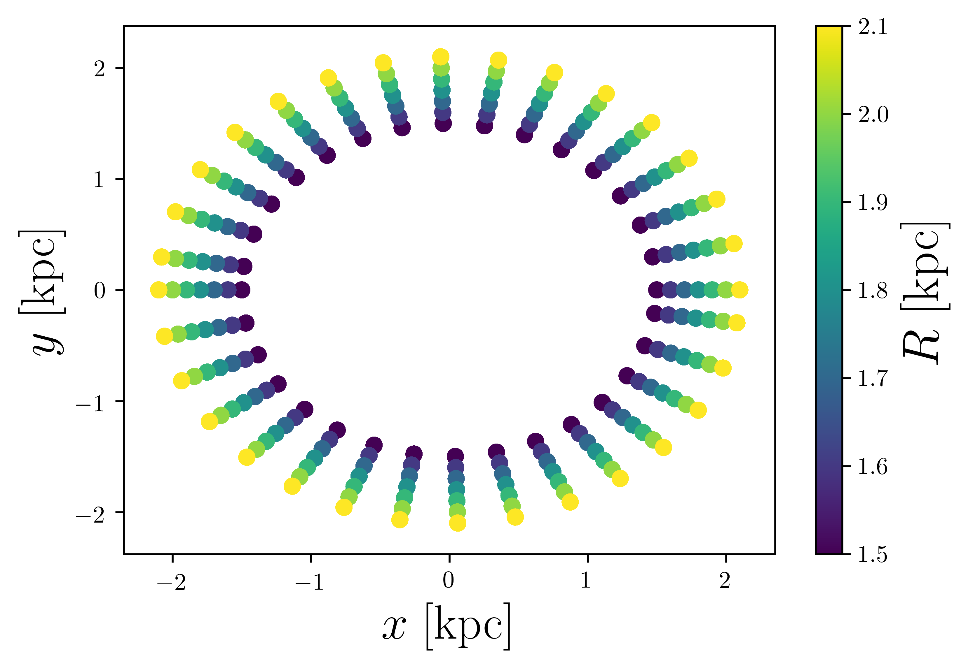
Figure 13: In this figure, we show the position of the ideal observers, sitting at rest on the galaxy disc, that we use to register the passage of the density perturbation driven by the spiral arms, by considering all available snapshots between redshift $z\approx 1.8$ to $z\approx 2.6$. Each individual observer defines a box with size of $0.1\,\text{kpc}$ around them.

The radial profiles of both the rotational and vertical velocity dispersions (middle and bottom panels of Fig. 8, respectively) are predicted be $\lesssim 60\,\text{km/s}$ on the disc. The central peak in $\sigma_{\text{rot}}$ is due to the bar, which – as aforementioned – has a strong effect on the gas kinematics, which is seen in our simulation in terms of a significant increase of the dispersion of the rotational and radial velocity components. The vertical velocity dispersion is not affected by the bar, being more sensitive to the physical conditions of the environment. Since the disc at $z=3$ has a smaller physical size than at $z=2$, the high values of $\sigma_{\text{vert}}$ at large $R$ at $z=3$ correspond to regions outside the main galaxy body. Fig. 8 also demonstrates that in our spiral galaxy, the thick disc formed before the thin disc.

Figure 14: The time evolution of the train of impulses in the gas density, due to the passage of the spiral arms, as seen by each observer of Fig. 13, according to its azimuth angle $\theta$. Each panel corresponds to the galactocentric distance of the observers, and the colour coding goes from $0$ to $1$, being normalised to the maximum number of particles (the maximum amplitude of the impulses) that each observer has ever seen passing through their region. We note that this figure is made by considering all snapshots available from redshift $z\approx 1.8$ (look-back time $t_{\text{lb}}=0$) to $z\approx 2.6$.

The vast majority of observations at redshift $z\sim 1-2$ have measured gas velocity dispersions of the order $\sigma_{v}\sim 40$-$80\;\text{km/s}$ for the thick component of galaxy discs (Genzel et al., 2008; Wisnioski et al., 2015), however, those are usually clumpy disc galaxies without obvious spiral structures. Spiral galaxies at similar redshifts likely have lower velocity dispersions ($\sigma_{v}\sim 20$-$40\;\text{km/s}$) (Yuan et al., 2017; Di Teodoro et al., 2018), with merger-triggered spirals representing an exception (Law et al., 2012). All nearby spirals systematically show low gas velocity dispersion and disc scale height (Epinat et al., 2010). Our simulation is consistent with the idea that long-lived density wave spiral arms reside in low-velocity dispersion thin discs (Yuan et al., 2017).

3.3 Kinematical properties of the stellar populations on the galaxy disc

In Fig. 9, we show how the full width at half maximum (FWHM) of the height distribution of the stellar populations in the galaxy, $\mathcal{P}(\lvert z_{\text{th}}\rvert)$, varies as a function of the age (top panel) and metallicity (bottom panel) of the galaxy stellar populations at redshift $z=2$. The black triangle in the top panel of Fig. 9 corresponds to the FWHM of the height distribution of the galaxy gas particles, which are predicted to reside on a very thin disc at $z=2$.

First of all, by looking at Fig. 9, as we consider older stellar populations, they typically cover larger ranges of galactic altitudes. Secondly, also the stellar metallicity is strongly correlated with the height distribution of the stars in the galaxy, with the metal-poor stars covering much wider ranges of galactic altitudes than the metal-rich stars, which are typically concentrated on thinner discs. Both age and metallicity dependencies are consistent with observations in the Milky Way (Ting & Rix, 2018; Mackereth et al., 2019), and also with predictions of the monolithic collapse scenario (e.g., Larson, 1974) and chemodynamical simulations (e.g., Kobayashi & Nakasato, 2011).

In Fig. 10, stellar populations of different ages are disentangled to show how their main kinematical properties vary as functions of their galactocentric distance. In particular, the various panels show the radial profile of the specific angular momentum of stars in different age bins (top panel), the radial profile of the rotational velocity dispersion (middle panel), and the radial profile of the vertical velocity dispersion (bottom panel). Fig. 10 shows that the old stellar populations are more dominated and supported by their random motions, having – at any galactocentric distance – lower specific angular momenta, and higher rotational and vertical velocity dispersions, than the young stellar populations. It is worth noting that the youngest stellar populations have very similar kinematical properties as the gas in the galaxy, at any galactocentric distances, since they both determine galaxy structures which are rotation-supported. The exponential profiles of the vertical velocity dispersion versus radius relation are consistent with local spiral galaxies (e.g., Aniyan et al. 2018).

3.4 Properties of the stars on the spiral arms

In Fig. 11, we show where the star formation activity takes place in our simulated disc galaxy, from $z=3$ down to $z=2$. In the background, with black dots, we show the spatial distribution of the gas particles in the galaxy, viewed edge-on, and we highlight in yellow all the star-forming gas particles in the galaxy. We find that the SFR is highest in the bar at all redshifts. The SFR is also high in clumps along the spiral arms of the galaxy. We also find more intense star formation activity along the spiral arms as the galaxy approaches redshift $z=2$, where there is the peak in the cosmic star formation rate (Madau & Dickinson, 2014). Our findings are in agreement with the observations in the local Universe, where the star formation activity usually takes place in dense molecular clouds along spiral arms (Schinnerer et al., 2013). In the present-day bulges, however, we do not have any evident sign of ongoing strong star formation activity in nearby disc galaxies, even though bulges are usually heavily obscured by dust extinction (Nelson et al., 2018).

Unlike the instantaneous snapshots of observed galaxies (§1), our simulated galaxy allows us to probe the origin of spiral arms. We did this by tracing the ID numbers of star particles, following the evolution of the spiral structures in the simulated galaxy. In Fig. 12, we quantify the fraction of the stellar populations residing on the spiral arms at different redshifts, by identifying the star particles on the spiral arms at different redshifts. If at two different redshifts we can prove that there are very different populations of stars on the spiral arms, then this is a signature of the fact that spiral arms in our simulated galaxy originate from density wave perturbations propagating on the galaxy disc, and that the spiral arms are not induced by mergers or accretion events.

The $y$-axis in Fig. 12 represents the fraction of stars on the spiral arms, in common between the time indicated by each colour (corresponding to the redshifts $z=2.0$, $2.2$, and $2.4$) and a set of previous epochs of the galaxy evolution. The $x$-axis of Fig. 12 represents the look-back time, starting from the time corresponding to the redshift when we compute $f_{\text{spiral}}$. In Fig. 12, we show the evolution of $f_{\text{spiral}}$ as a function the look-back time, by considering only the stellar populations with B-band luminosity, $l_{\text{B},\star}$, satisfying the following condition:

$$\log(l_{\text{B},\star}/l_{\text{B},\sun})>{3.5}.$$ (1)

Even if we considered either all the stellar populations on the arms (regardless their age, metallicity, B-band luminosity, and so on), or the stellar populations following equation 1, we find results very similar as those shown in Fig. 12.

Fig. 12 shows that – as the spiral pattern rotates – there are always different stellar populations on the spiral arms. In particular, the fraction of stars on the spiral arms in common between different redshifts, $f_{\text{spiral}}$, rapidly decreases as a function of the look-back time, being $<15$ per cent for $\Delta t\approx 0.1\,\text{Gyr}$, and as low as $5$ per cent for $\Delta t\approx 0.5\,\text{Gyr}$, whatever be the initial redshift we consider for reference. If we fit with a decaying exponential function $f_{\text{spiral}}$ as a function of the look-back time in Fig. 12, we predict a decay time-scale $\tau_{\text{spiral}}\approx 193\,\text{Myr}$, over which the stellar populations typically leave the spiral arm, where they were born.

We remark on the fact that the young stellar populations on the spiral arms have initially very similar kinematics as the gas on the galaxy disc (see Fig. 7, where stars with ages $<0.5\,\text{Gyr}$ have similar kinematical properties as the gas), with an average radial velocity component which is consistent with $\approx 0\,\text{km}\,\text{s}^{-1}$ (see Fig. 10); therefore, the evolution of $f_{\text{spiral}}$ as a function of the look-back time in Fig. 12 is not an artifact of the epicyclic motion of stars.

In conclusion, we find that the spiral arms in our simulated high-redshift disc galaxy typically host star-forming gas particles and young stellar populations; moreover, spiral arms are like a perturbation, which propagates on the galaxy disc with a different angular velocity than that of the gas and stars on the disc.

4 The angular velocity of the spiral arms

Whether we are dealing with classical (e.g., Lin & Shu 1964) or kinematical (e.g., Dobbs et al. 2010) spiral density waves or with manifold-driven spiral arms (Athanassoula, 2012), the angular velocity of the spiral pattern perturbation should appear constant as a function of galactocentric distance. In other words, while the stars and gas on the disc show differential angular rotation, the spiral pattern should move like a solid body, with constant radial profile for the angular rotation velocity. In this Section, we investigate all these aspects by looking at the properties of the spiral pattern at different epochs of the galaxy evolution in our simulation.

First of all, we place many ideal observers at different galactocentric distances, $r$, and azimuth angles, $\theta$, sitting at rest on the galaxy disc; the position of these observers is shown in Fig. 13. Each individual observer then registers the train of impulses as a function of time, as due to the passage of the spiral arm density perturbation. We assume that each observer defines a box region around them with size $0.1\,\text{kpc}$.

In Figure 14, we show the time evolution of the train of impulses in the gas density, as registered by the observers of Fig. 13, covering different azimuth angles and distances on the galaxy disc. We consider all available snapshots, from redshift $z\approx 1.8$ to $z\approx 2.6$, with the zero point for the look-back time corresponding to redshift $z\approx 1.8$. Each panel in Fig. 14 corresponds to different galactocentric distances, and – within each panel – the colour-coding represents the normalised number of particles, $\mathcal{N}(r,\theta,t)$, that each observer sees at the given look-back time, where the normalisation factor, $\mathcal{A}(r,\theta)$, corresponds to the maximum impulse in the density perturbation that each observer has ever seen in the considered redshift range.

We can use Fig. 14 to compute the angular velocity of the spiral pattern:

$$\Omega_{\text{spiral}}(r)=\Big{(}\frac{d\theta(r)}{dt}\Big{)}_{\text{spiral}},$$ (2)

which may depend – in principle – on the galactocentric distance and time. We note that, just by overplotting the different panels of Fig. 14, we can see that the various patterns of $\theta$ versus time match with each other for different galactocentric distances, meaning – qualitatively – that the spiral structure perturbation rotates on the disc like a solid body; nevertheless, we would like to develop a simple analysis to quantify more precisely $\Omega_{\text{spiral}}(r)$ on the galaxy disc.

Figure 15: The time evolution of the spiral pattern angular velocity as a function of the galactocentric distance, as determined from the analysis of Fig. 14, by computing the slopes of $\theta(r)$ versus time, in different ranges of time in the past, for different galactocentric distances, $r$.

In order to quantify $\Omega_{\text{spiral}}(r)$, we have computed the slopes of $\theta$ versus $t$ in Fig. 14, by fitting – for different galactocentric distances – the predicted $\theta$–time relations of the overdensities, assuming a simple linear relation. The time evolution of $\Omega_{\text{spiral}}(r)$ is then simply obtained by fitting the predicted $\theta$–time relations of the overdensities in different time intervals. The results of our analysis are shown in Fig. 15, where different colours correspond to different intervals in the look-back time. Finally, the error bars in Fig. 15 correspond to the errors in the best fit parameters, with the shaded coloured areas representing the average angular velocity (with the corresponding $\pm 1\sigma$ deviations), in the considered time interval.

The main findings of our analysis are that (i) $\Omega_{\text{spiral}}$ is almost constant on the main body of the galaxy gaseous disc; (ii) $\Omega_{\text{spiral}}$ increases, on average, as a function of time, which is consistent with the increase of the specific angular momentum as a function of time, seen in Fig. 8. The pattern speed of spiral arms is considered an important feature in secular evolution of disc galaxies (Buta & Zhang, 2009) and is related to the angular momentum transport within the disc (Lynden-Bell & Kalnajs, 1972). In our simulated galaxy, we have continuous gas accretion, which deposit kinetic energy and momentum onto the galaxy disc, enhancing its specific angular momentum as a function of time, particularly in the outer galaxy regions, which are less gravitationally bound; at the same time, the spiral pattern perturbation keeps its constant radial profile as a function of radius.

We note that our estimated values for $\Omega_{\text{spiral}}$ rely on the assumption that we can fit the predicted $\theta$ versus $t$ relations of the overdensities with a simple linear relation; this is the main source of error in our analysis, since it is clear – just by looking at Fig. 14 – that the slope of $\theta$ versus $t$ slightly changes with time, particularly at high-redshifts, when the galaxy disc is developing; moreover, there are also many local, sudden inhomogeneities appearing on the galaxy disc. All these effects are taken into account in the error estimate of $\Omega_{\text{spiral}}$. Nevertheless, we acknowledge that a more precise analysis – measuring the instantaneous $\Omega_{\text{spiral}}$ – would link the evolution of $\Omega_{\text{spiral}}$ to disturbance events from external (e.g., accretion of substructures through the filaments) or internal sources (e.g., star formation activity and feedback).

Figure 16: The radial profile of the angular velocity of the gas (blue points with errorbars) on the galaxy disc of our simulated disc galaxy at redshift $z\approx 2$.

Figure 17: The first column shows the spiral arms (top panel) and the bar (bottom panel) at different epochs of the galaxy evolution in the $r$-$\theta$ diagram, where $r$ represents the galactocentric distance and $\theta$ the azimuthal angle. The second column shows the spiral arms (top panel) and the bar (bottom panel) at three epochs (blue, orange, and red points), with the galaxy being viewed face-on in the $x$-$y$ plane.

The angular velocity of the spiral pattern (see Fig. 15) is much slower than the circular motion of the gas on the disc, which is shown in Fig. 16. This can be better appreciated by computing the co-rotation radius, $r_{\text{cr}}$, which is defined as the galactocentric distance, where the following equivalence is satisfied.

$$\Omega_{\star}(r_{\text{cr}})=\frac{v_{\text{circ}}}{r_{\text{cr}}}\equiv\Big{(}\frac{d\theta}{dt}\Big{)}_{\text{spiral}},$$ (3)

where $\Omega_{\star}$ represents the angular velocity of the stellar populations on the galaxy disc. If we assumed a flat rotation curve which extends well beyond the physical dimensions of our simulated galaxy at $z=2$, then we would have a co-rotation radius $r_{\text{cr}}\approx 13\,\text{kpc}$.

We notice from Fig. 5 and Fig. 8 that the spiral pattern changes from less regular to fully organised when the gas settles from a thick (with vertical dispersion $\sigma_{v}>$ 50 km/s) to a thin ($\sigma_{v}\sim 25$ km/s) disc component from $z\sim 3$ to $z\sim 2$. This co-evolution of spiral arms and thin discs is expected in density wave theories of spiral arm formation (e.g., Lin & Shu 1964; Bottema 2003; Sellwood 2014).

Manifold theory (Athanassoula, 2012) may also be a good alternative explanation for the origin of the spiral arms, and for the constancy of their angular velocity as a function of radius, since the spiral pattern in our simulation is seen – at all redshifts – to co-rotate with the strong central bar (see Fig. 17). In this scenario, the gas naturally accumulates in invariant manifolds, which are defined as regions around the unstable Lagrange points of the bar, co-rotating with the bar. Nevertheless, we remark on the fact that the gas and stars particles in our simulation have intrinsically higher angular velocity than the spiral pattern at the same radius (see Fig. 16). A more careful analysis is needed to disentangle between the kinematic density-wave theory and the manifold theory, because both of them could give rise to a constant pattern speed as a function of radius. We leave this study to a future work, in which we will perform accurate orbital analysis of the star particles in our simulations, by also making use of other available codes (e.g., Bovy 2015).

5 Conclusions

In this paper, we have presented the results of our zoom-in cosmological chemodynamical simulation, which unintentionally demonstrated the formation and evolution of a star-forming, barred spiral galaxy from redshift $z\sim 3$ to $z\sim 2$.

At redshift $z=2$, the simulated galaxy in our zoom-in simulation has a total stellar mass $M_{\star}=4.16\times 10^{10}\,\text{M}_{\sun}$, total gas mass $M_{\text{gas}}=9.03\times 10^{9}\,\text{M}_{\sun}$, V-band half-light radius $\sim 3$ kpc, disc scale height $\sim 0.36$ kpc, and the average circular velocity $\langle v_{\text{circ}}=\rangle 287.0\pm 12.3\,\text{km/s}$, and hence it is a thin disc galaxy. The average stellar and gas-phase metallicities are $\log(Z_{\star}/Z_{\sun})=-0.24$ and $\log(Z_{\text{gas}}/Z_{\sun})=-0.30$, respectively, and the metallicity evolution is driven by a large-scale primordial gas accretion (Fig. 3). Our study demonstrates that high-resolution cosmological hydrodynamical simulations are now ready to examine the formation and evolution of high-redshift spiral galaxies in the same detailed manner as of nearby spiral galaxies. Our main conclusions can be summarised as follows.

1. The seed of our simulated disc galaxy is represented by the central “bulge”, which formed at high redshift from the assembly of many dense, gas-rich clumps. Following the size growth of the disc, the galaxy develops from redshift $z\approx 3.5$, with two trailing spiral arms being present down to redshift $z\approx 1.8$.

2. By identifying star particles during the evolution of the spiral structure, we find that the spiral arms originate from density wave perturbations. The stellar populations newly-born in the arms leave the spiral arms over an average typical time-scale $\tau_{\text{spiral}}\approx 193\,\text{Myr}$, irrespective of redshift (Fig. 11).

3. The pattern of the spiral arms rotates like a solid body, propagating like a perturbation on the galaxy disc, with relatively low constant angular velocity (approximately three rotations per Gyr), setting the galaxy co-rotation radius at $13.6\,\text{kpc}$ (Fig. 12).

4. The central bulge is constituted by an X-shaped bar, with the orbits of the particles in the simulation following a “figure of eight” as a function of time. The bar formed by $z\sim 3$ and the presence of the bar determines an increase (i.e. a heating) of the radial velocities of the gas particles in the galaxy centre.

5. The star formation activity in our simulated disc galaxy takes place in the central bulge and in several clumps on the spiral arms, at all redshifts. The number and size of the star-forming gas clumps on the arms increases as a function of redshift, reaching a maximum at $z\approx 2$, when we have the peak of the cosmic SFR.

6. By analysing the kinematic properties of stellar populations with different age in the galaxy, we find that stellar populations with increasing age are concentrated, on average, towards higher galactic latitudes and have also lower average metallicities. The old stellar populations have lower specific angular momentum and higher velocity dispersion than the young ones, at all galactocentric distances.

7. The specific angular momentum of the gas on the galaxy thin disc increases as a function of redshift, with the angular velocity of the spiral pattern, $\Omega_{\text{spiral}}$, keeping always its radial profile constant. The velocity dispersion in the thin disc remains always lower, on average, than $\sim 50\,\text{km/s}$.

8. The dynamical structure of the spiral arms in the simulation is different than that of the bulk of the stars and gas on the galaxy disc; in particular, $\Omega_{\text{spiral}}$ increases as function of time (like the specific angular momentum of the gas in the disc), maintaining a profile which is constant as a function of radius. This suggests that the spiral pattern is a fundamental process with which angular momentum is transported within our simulated disc galaxy (Lynden-Bell & Kalnajs, 1972). Nevertheless, with our current analysis, we cannot robustly disentangle between kinematic density waves and manifold theory for the origin of the spiral arms, because both theories can give rise to a constant radial profile of the angular velocity of the spiral pattern on the galaxy disc; this will be the subject of our future work

References

- Abadi et al. (2003) Abadi, M. G. et al., 2003, ApJ, 591, 499
- Agertz, Teyssier & Moore (2009) Agertz O., Teyssier R., Moore B., 2009, MNRAS, 397, L64
- Agertz, Teyssier & Moore (2011) Agertz O., Teyssier R., Moore B., 2011, MNRAS, 410, 1391
- Allen et al. (2008) Allen, M. G., Groves, B. A., Dopita, M. A., Sutherland, R. S., & Kewley, L. J. 2008, ApJS, 178, 20
- Alves de Oliveira et al. (2018) Alves de Oliveira, C., Birkmann, S. M., Böker, T., et al. 2018, Observatory Operations: Strategies, Processes, and Systems VII, 10704, 107040Q
- Aniyan et al. (2018) Aniyan, S., Freeman, K. C., Arnaboldi, M., et al. 2018, MNRAS, 476, 1909.
- Asplund et al. (2009) Asplund, M., Grevesse, N., Sauval, A. J., & Scott, P. 2009, ARA&A, 47, 481
- Athanassoula (2012) Athanassoula E., 2012, MNRAS, 426, L46
- Aumer et al. (2013) Aumer M., White S. D. M., Naab T., Scannapieco C., 2013, MNRAS, 434, 3142
- Baba, Saitoh & Wada (2013) Baba J., Saitoh T. R., Wada K., 2013, ApJ, 763, 46
- Baes et al. (2003) Baes, M., Davies, J. I., Dejonghe, H., et al. 2003, MNRAS, 343, 1081
- Baes et al. (2011) Baes, M., Verstappen, J., De Looze, I., et al. 2011, ApJS, 196, 22
- Benson (2010) Benson, A. J. 2010, Phys. Rep., 495, 33.
- Binney & Tremaine (2008) Binney, J., & Tremaine, S. 2008, Princeton University Press, Princeton, NJ USA
- Bonnet et al. (2004) Bonnet, H., Abuter, R., Baker, A., et al. 2004, The Messenger, 117, 17
- Bottema (2003) Bottema, R. 2003, MNRAS, 344, 358.
- Bovy (2015) Bovy J., 2015, ApJS, 216, 29
- Bundy et al. (2015) Bundy, K., Bershady, M. A., Law, D. R., et al. 2015, ApJ, 798, 7
- Buta & Zhang (2009) Buta, R. J. & Zhang, X. 2009, ApJS, 182, 559
- Camps & Baes (2015) Camps, P., & Baes, M. 2015, Astronomy and Computing, 9, 20
- Cappellari (2016) Cappellari M., 2016, ARA&A, 54, 597
- Catelan, & Theuns (1996) Catelan, P., & Theuns, T. 1996, MNRAS, 282, 436.
- Cen (2014) Cen, R. 2014, ApJ, 789, L21.
- Chabrier (2003) Chabrier, G. 2003, PASP, 115, 763
- Comparetta & Quillen (2012) Comparetta J., Quillen A. C., 2012, arXiv e-prints, arXiv:1207.5753
- Conselice (2014) Conselice, C. J. 2014, ARA&A, 52, 291
- Clauwens et al. (2018) Clauwens, B., Schaye, J., Franx, M., et al. 2018, MNRAS, 478, 3994.
- Colín et al. (2016) Colín P., Avila-Reese V., Roca-Fàbrega S., Valenzuela O., 2016, ApJ, 829, 98
- Croom et al. (2012) Croom, S. M., Lawrence, J. S., Bland-Hawthorn, J., et al. 2012, MNRAS, 421, 872
- Davis et al. (2015) Davis, B. L., Kennefick, D., Kennefick, J., et al. 2015, ApJ, 802, L13
- Davis et al. (2017) Davis, B. L., Graham, A. W., & Seigar, M. S. 2017, MNRAS, 471, 2187
- Di Teodoro et al. (2018) Di Teodoro, E. M., Grillo, C., Fraternali, F., et al. 2018, MNRAS, 476, 804
- Dobbs & Baba (2014) Dobbs, C., & Baba, J. 2014, Publ. Astron. Soc. Australia, 31, e035
- Dobbs et al. (2010) Dobbs, C. L., Theis, C., Pringle, J. E., & Bate, M. R. 2010, MNRAS, 403, 625
- D’Onghia, Vogelsberger & Hernquist (2013) D’Onghia E., Vogelsberger M., Hernquist L., 2013, ApJ, 766, 34
- Efthymiopoulos, Kyziropoulos, Páez, Zouloumi & Gravvanis (2019) Efthymiopoulos C., Kyziropoulos P. E., Páez R. I., Zouloumi K., Gravvanis G. A., 2019, MNRAS, 484, 1487
- Epinat et al. (2008) Epinat, B., Amram, P., Marcelin, M., et al. 2008, MNRAS, 388, 500.
- Epinat et al. (2010) Epinat, B., Amram, P., Balkowski, C., & Marcelin, M. 2010, MNRAS, 401, 2113
- Faesi et al. (2018) Faesi, C. M., Lada, C. J., & Forbrich, J. 2018, ApJ, 857, 19
- Förster Schreiber et al. (2009) Förster Schreiber, N. M., Genzel, R., Bouché, N., et al. 2009, ApJ, 706, 1364
- Freeman, & Bland-Hawthorn (2002) Freeman, K., & Bland-Hawthorn, J. 2002, Annual Review of Astronomy and Astrophysics, 40, 487.
- Fujii et al. (2011) Fujii M. S., Baba J., Saitoh T. R., Makino J., Kokubo E., Wada K., 2011, ApJ, 730, 109
- Genel et al. (2015) Genel, S., Fall, S. M., Hernquist, L., et al. 2015, ApJ, 804, L40.
- Genzel et al. (2008) Genzel, R., Burkert, A., Bouché, N., et al. 2008, ApJ, 687, 59
- Glazebrook (2013) Glazebrook, K. 2013, Publications of the Astronomical Society of Australia, 30, e056.
- Goldreich & Lynden-Bell (1965) Goldreich, P., & Lynden-Bell, D. 1965, MNRAS, 130, 125
- Graham & Worley (2008) Graham, A. W., & Worley, C. C. 2008, MNRAS, 388, 1708
- Grand, Kawata & Cropper (2012) Grand R. J. J., Kawata D., Cropper M., 2012, MNRAS, 421, 1529
- Grand, et al. (2015) Grand R. J. J., et al., 2015, MNRAS, 453, 1867
- Grand, et al. (2017) Grand R. J. J., et al., 2017, MNRAS, 467, 179
- Guedes et al. (2011) Guedes J., Callegari S., Madau P., Mayer L., 2011, ApJ, 742, 76
- Haardt & Madau (haardt1996) Haardt, F., & Madau, P. 1996, ApJ, 461, 20
- Hahn & Abel (2011) Hahn, O., & Abel, T. 2011, MNRAS, 415, 2101
- Haywood et al. (2016) Haywood, M., Lehnert, M. D., Di Matteo, P., et al. 2016, A&A, 589, A66.
- Bland-Hawthorn & Gerhard (2016) Bland-Hawthorn, J., & Gerhard, O. 2016, Annual Review of Astronomy and Astrophysics, 54, 529.
- Hodge et al. (2018) Hodge, J. A., Smail, I., Walter, F., et al. 2018, arXiv e-prints , arXiv:1810.12307.
- Hopkins, Kereš & Murray (2013) Hopkins P. F., Kereš D., Murray N., 2013, MNRAS, 432, 2639
- Hubble (1926) Hubble, E. P. 1926, ApJ, 64, 321.
- Hu & Sijacki (2016) Hu S., Sijacki D., 2016, MNRAS, 461, 2789
- Julian & Toomre (1966) Julian, W. H., & Toomre, A. 1966, ApJ, 146, 810
- Kalnajs (1971) Kalnajs, A. J. 1971, ApJ, 166, 275
- Kalnajs (1973) Kalnajs A. J., 1973, PASAu, 2, 174
- Katz & Gunn (1991) Katz N., Gunn J. E., 1991, ApJ, 377, 365
- Katz (1992) Katz, N. 1992, ApJ, 391, 502
- Katz et al. (1996) Katz, N., Weinberg, D. H., & Hernquist, L. 1996, ApJS, 105, 19
- Kobayashi (2004) Kobayashi C., 2004, MNRAS, 347, 740
- Kobayashi et al. (2007) Kobayashi C., Springel V., White S. D. M., 2007, MNRAS, 376, 1465
- Kobayashi & Nomoto (2009) Kobayashi, C., & Nomoto, K. 2009, ApJ, 707, 1466
- Kobayashi & Nakasato (2011) Kobayashi C., Nakasato N., 2011, ApJ, 729, 16
- Kobayashi et al. (2011) Kobayashi C., Karakas A. I., Umeda H., 2011, MNRAS, 414, 3231
- Koribalski et al. (2018) Koribalski, B. S., Wang, J., Kamphuis, P., et al. 2018, MNRAS, 478, 1611
- Kormendy & Norman (1979) Kormendy, J., & Norman, C. A. 1979, ApJ, 233, 539
- Kormendy (2016) Kormendy, J. 2016, Galactic Bulges, 418, 431
- Kregel & van der Kruit (2005) Kregel, M., & van der Kruit, P. C. 2005, MNRAS, 358, 481
- Kroupa (2008) Kroupa, P., 2008, Pathways Through an Eclectic Universe, 390, 3
- Lagos et al. (2017) Lagos, C. del P., Theuns, T., Stevens, A. R. H., et al. 2017, MNRAS, 464, 3850.
- Law et al. (2012) Law, D. R., Shapley, A. E., Steidel, C. C., et al. 2012, Nature, 487, 338
- Larson (1974) Larson, R. B. 1974, MNRAS, 166, 585
- Law et al. (2012) Law, D. R., Steidel, C. C., Shapley, A. E., et al. 2012, ApJ, 759, 29
- Lin & Shu (1964) Lin, C. C., & Shu, F. H. 1964, ApJ, 140, 646
- Lin & Shu (1966) Lin, C. C., & Shu, F. H. 1966, Proceedings of the National Academy of Science, 55, 229
- Lindblad (1960) Lindblad, P. O. 1960, Stockholms Observatoriums Annaler, 21
- Lynden-Bell & Kalnajs (1972) Lynden-Bell, D. & Kalnajs, A. J. 1972, MNRAS, 157, 1
- Mackereth et al. (2019) Mackereth, J. T., Bovy, J., Leung, H. W., et al. 2019, arXiv:1901.04502
- Madau & Dickinson (2014) Madau, P., & Dickinson, M. 2014, ARA&A, 52, 415
- Marinacci, Pakmor & Springel (2014) Marinacci F., Pakmor R., Springel V., 2014, MNRAS, 437, 1750
- Marsh et al. (2018) Marsh, K. A., Whitworth, A. P., Smith, M. W. L., Lomax, O., & Eales, S. A. 2018, MNRAS, 480, 3052
- Masset & Tagger (1997) Masset, F., & Tagger, M. 1997, A&A, 322, 442
- Monaghan (1992) Monaghan, J. J. 1992, ARA&A, 30, 543
- Mosenkov et al. (2018) Mosenkov, A. V., Allaert, F., Baes, M., et al. 2018, A&A, 616, A120
- Navarro & Steinmetz (2000) Navarro J. F., Steinmetz M., 2000, ApJ, 538, 477
- Nelson et al. (2018) Nelson, E. J., Tadaki, K.-i., Tacconi, L. J., et al. 2018, arXiv:1801.02647
- Oh, Kim, Lee & Kim (2008) Oh S. H., Kim W.-T., Lee H. M., Kim J., 2008, ApJ, 683, 94
- Oh, Kim & Lee (2015) Oh S. H., Kim W.-T., Lee H. M., 2015, ApJ, 807, 73
- Peterken et al. (2018) Peterken, T. G. et al. 2018, arXiv:1809.08048
- Planck Collaboration et al. (2016) Planck Collaboration, Ade, P. A. R., Aghanim, N., et al. 2016, A&A, 594, A13
- Planck Collaboration et al. (2018) Planck Collaboration, Aghanim, N., Akrami, Y., et al. 2018, arXiv:1807.06209
- Posselt et al. (2004) Posselt, W., Holota, W., Kulinyak, E., et al. 2004, Proc. SPIE, 5487, 688
- Price (2012) Price, D. J., 2012, Journal of Computational Physics, 231, 759
- Quillen et al. (2011) Quillen A. C., Dougherty J., Bagley M. B., Minchev I., Comparetta J., 2011, MNRAS, 417, 762
- Rix & Rieke (1993) Rix, H.-W., & Rieke, M. J. 1993, ApJ, 418, 123
- Rix & Bovy (2013) Rix, H.-W., & Bovy, J. 2013, Astronomy and Astrophysics Review, 21, 61.
- Rosswog (2009) Rosswog, S. 2009, New Astron. Rev., 53, 78
- Salo & Laurikainen (1993) Salo, H., & Laurikainen, E. 1993, ApJ, 410, 586
- Sánchez et al. (2016) Sánchez, S. F., García-Benito, R., Zibetti, S., et al. 2016, A&A, 594, A36
- Sánchez-Menguiano et al. (2017) Sánchez-Menguiano, L., Sánchez, S. F., Pérez, I., et al. 2017, A&A, 603, A113
- Scannapieco et al. (2008) Scannapieco C., Tissera P. B., White S. D. M., Springel V., 2008, MNRAS, 389, 1137
- Scannapieco et al. (2012) Scannapieco, C., Wadepuhl, M., Parry, O. H., et al. 2012, MNRAS, 423, 1726
- Schinnerer et al. (2013) Schinnerer, E., Meidt, S. E., Pety, J., et al. 2013, ApJ, 779, 42
- Schinnerer et al. (2017) Schinnerer, E., Meidt, S. E., Colombo, D., et al. 2017, ApJ, 836, 62
- Sellwood & Carlberg (1984) Sellwood, J. A., & Carlberg, R. G. 1984, ApJ, 282, 61
- Sellwood & Binney (2002) Sellwood J. A., Binney J. J., 2002, MNRAS, 336, 785
- Sellwood (2014) Sellwood, J. A. 2014, Reviews of Modern Physics, 86, 1.
- Sellwood & Carlberg (2014) Sellwood J. A., Carlberg R. G., 2014, ApJ, 785, 137
- Sharma et al. (2018) Sharma, S., Richard, J., Yuan, T., et al. 2018, MNRAS, 481, 1427.
- Springel et al. (2001) Springel, V., Yoshida, N., & White, S. D. M. 2001, New Astron., 6, 79
- Springel (2005) Springel V., 2005, MNRAS, 364, 1105
- Steinmetz & Navarro (1999) Steinmetz M., Navarro J. F., 1999, ApJ, 513, 555
- Stinson et al. (2013) Stinson G. S., et al., 2013, MNRAS, 436, 625
- Stott et al. (2016) Stott, J. P., Swinbank, A. M., Johnson, H. L., et al. 2016, MNRAS, 457, 1888
- Struck, Dobbs & Hwang (2011) Struck C., Dobbs C. L., Hwang J.-S., 2011, MNRAS, 414, 2498
- Sun et al. (2018) Sun, J., Leroy, A. K., Schruba, A., et al. 2018, ApJ, 860, 172
- Sutherland & Dopita (1993) Sutherland, R. S., & Dopita, M. A. 1993, ApJS, 88, 253
- Tacconi et al. (2013) Tacconi, L. J., Neri, R., Genzel, R., et al. 2013, ApJ, 768, 74
- Taylor & Kobayashi (2014) Taylor, P., & Kobayashi, C. 2014, MNRAS, 442, 2751
- Thornley (1996) Thornley, M. D. 1996, ApJ, 469, L45
- Ting & Rix (2018) Ting, Y.-S., & Rix, H.-W. 2018, arXiv:1808.03278
- Toomre (1981) Toomre, A. 1981, Structure and Evolution of Normal Galaxies, 111
- Tremblay et al. (2014) Tremblay, P.-E., Kalirai, J. S., Soderblom, D. R., Cignoni, M., & Cummings, J. 2014, ApJ, 791, 92
- Trussler et al. (2018) Trussler, J., Maiolino, R., Maraston, C., et al. 2018, arXiv:1811.09283
- Übler et al. (2014) Übler H., Naab T., Oser L., Aumer M., Sales L. V., White S. D. M., 2014, MNRAS, 443, 2092
- Übler, et al. (2017) Übler H., et al., 2017, ApJ, 842, 121
- Vincenzo et al. (2016) Vincenzo, F., Matteucci, F., de Boer, T. J. L., Cignoni, M., & Tosi, M. 2016, MNRAS, 460, 2238
- Vincenzo & Kobayashi (2018a) Vincenzo, F., & Kobayashi, C. 2018, A&A, 610, L16
- Vincenzo & Kobayashi (2018b) Vincenzo, F., & Kobayashi, C. 2018, MNRAS, 478, 155
- Wada, Baba & Saitoh (2011) Wada K., Baba J., Saitoh T. R., 2011, ApJ, 735, 1
- Walter et al. (2008) Walter, F., Brinks, E., de Blok, W. J. G., et al. 2008, AJ, 136, 2563
- Willett et al. (2013) Willett, K. W., Lintott, C. J., Bamford, S. P., et al. 2013, MNRAS, 435, 2835.
- Wilson (2018) Wilson, C. D. 2018, MNRAS, 477, 2926
- Wisnioski et al. (2015) Wisnioski, E., Förster Schreiber, N. M., Wuyts, S., et al. 2015, ApJ, 799, 209
- Yu et al. (2018) Yu, S.-Y., Ho, L. C., Barth, A. J., & Li, Z.-Y. 2018, ApJ, 862, 13
- Yuan et al. (2017) Yuan, T., Richard, J., Gupta, A., et al. 2017, ApJ, 850, 61