H-T Phase Diagram of Rare-Earth – Transition Metal Alloy in the Vicinity of the Compensation Point

Abstract

Anomalous hysteresis loops of ferrimagnetic amorphous alloys in high magnetic field and in the vicinity of the compensation temperature have so far been explained by sample inhomogeneities. We obtain H-T magnetic phase diagram for ferrimagnetic GdFeCo alloy using a two-sublattice model in the paramagnetic rare-earth ion approximation and taking into account rare-earth (Gd) magnetic anisotropy. It is shown that if the magnetic anisotropy of the $f$-sublattice is larger than that of the $d$-sublattice, the tricritical point can be at higher temperature than the compensation point. The obtained phase diagram explains the observed anomalous hysteresis loops as a result of high-field magnetic phase transition, the order of which changes with temperature. It also implies that in the vicinity of the magnetic compensation point the shape of magnetic hysteresis loop is strongly temperature dependent.

I Introduction

Rare-earth amorphous alloys and intermetallics is a large class of magnetic materials allowing to change their magnetic properties in a wide range by a subtle change of the composition, temperature or application of magnetic field Buschow (1977); Franse and Radwański (1993); Belov et al. (1976); Duc et al. (2002); Sechovskỳ et al. (1994). The materials have already found applications as hard magnets or recording media and they still offer a rich playground in the areas of spintronics Žutić et al. (2004), magnonics Kruglyak et al. (2010) and ultrafast magnetism Stanciu et al. (2007a); Vahaplar et al. (2009); Moser et al. (2002); Ostler et al. (2012); Khorsand et al. (2012); Radu et al. (2011); Graves et al. (2013); Stanciu et al. (2007b); Le Guyader et al. (2012); Xu et al. (2010).

GdFeCo is a particular example of such amorphous alloys. It is a 3$d$-4$f$ ferrimagnet with compensation temperature Taylor and Gangulee (1980), at which the magnetizations of the two sublattices become equal. At temperatures lower than the compensation temperature, the magnetization of the rare-earth (Gd) sublattice $M_{f}$ is larger than that of the transition metal (Fe) $M_{d}$ ($M_{f}-M_{d}>0$), whereas at higher temperatures $M_{f}-M_{d}<0$. Many studies of GdFeCo, GdFe and GdCo compounds as well as magnets with different rare-earth ion in high magnetic field revealed triple hysteresis loops in the vicinity of the magnetization compensation point Esho (1976); Chen and Malmhäll (1983); Okamoto and Miura (1989); Amatsu et al. (1977); Becker et al. (2017). The observed triple loops are clearly different from a hysteresis loop normally expected for a single thin film, where one would not expect a sudden decrease in magnetization in the strong applied magnetic field. However, hysteresis loops of this form are typical for multilayered structures. To emphasize the difference, we will refer to the the loops in single-layer structures as anomalous. These loops are strongly dependent on temperature. Earlier similar behavior was explained by sample inhomogeneities Amatsu et al. (1977) or strong exchange bias between surface and bulk layers that have different stochiometric composition of the alloy; in particular, this lead to estimation of the strongest ever reported exchange bias field of several Tesla Chen et al. (2015). However, to date no theoretical model has been proposed that would allow to calculate magnetization curves that would explain experimental data. Here we use a model for a homogeneous two-sublattice ferrimagnet film and suggest an alternative explanation for the observed anomalous hysteresis loops.

Figure 1 shows the results of high magnetic field measurements of the magneto-optical Kerr effect in GdFeCo Becker et al. (2017). The composition of the alloy with 24 $\%$ Gd, 66.5 $\%$ Fe and 9.5 $\%$ Co resulted in the compensation temperature $T_{comp}$=283 K. The field was applied at the normal to the sample, which is also the easy magnetization axis. The measurements were done at the probe wavelength of 630 nm in the polar Kerr geometry. In this case the probe is predominantly sensitive to the magnetization of the Fe-sublattice. Therefore the obtained hysteresis loops reveal the field dependence of the orientation of the Fe-magnetization. It is seen upon an increase of the field first a minor hysteresis loop shows up, which corresponds to the magnetization reversal. Further increase of the field does not change the orientation of the magnetization until a critical field is reached. This field launches spin-flop transition which is seen as a decrease of the magneto-optical signal. At this field the magnetizations of the sublattices turn from the normal of the sample, get canted and form a non-collinear state. The character of the spin-flop transition changes with temperature. Below the magnetic compensation temperature the spin-flop transition occurs gradually (see loops for 260 K and 277 K in Fig. 1). Just above the compensation point at the spin-flop field one observes abrupt change in the magnetic structure (see loops for 289 K and 291 K in Fig. 1). Upon further increase of the sample temperature the transition is seen as gradual again (see loop at 321 K in Fig. 1). Abrupt and gradual changes in magnetization induced by external magnetic field are characteristic features of first- and second-order phase transitions, respectively. Hence, these measurements imply that the order of the phase transition changes from second to first and back to second upon a temperature increase across the compensation point. Such a temperature-dependent order of the spin-flop transition has not been described for GdFeCo in literature before.

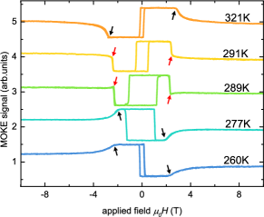
Figure 1: Static magneto-optic Kerr effect in GdFeCo sample measured at 630 nm probe wavelength at different temperatures from 260 to 321 K. A paramagnetic background was subtracted from the measurements. The compensation temperature is 283 K. Ref. Becker et al. (2017). Black and red arrows indicate second- and first-order transitions, respectively.

Note that, although phase diagrams for 3$d$-4$f$ ferrimagnets were first obtained theoretically almost 50 years ago Goransky and Zvezdin (1969); Zvezdin and Matveev (1972) and supported by numerous experiments (see [Zvezdin, 1995] and references therein), in the studies performed so far the anisotropy of the transition metal sublattice was taken to be larger than that of the rare-earth sublattice. The existing results on the magnetic phase diagrams fail to explain the anomalous hysteresis loops observed experimentally Amatsu et al. (1977); Becker et al. (2017); Chen et al. (2015). Unusual behavior of the critical fields in rare-earth intermetallics in the case of prevailing anisotropy of the rare-earth sublattice was recently investigated by some of co-authors theoretically for HoFe_xAl_12-x Sabdenov et al. (2017a, b). Here we show that if the rare-earth anisotropy is larger than that of the transition metal, the tricritical point on the phase diagram lies at higher temperatures with respect to the compensation point. As a result, the observed hysteresis loops can be explained in terms of intrinsic first- and second-order phase transitions in the intermetallic samples.

II Magnetic phase diagram

To obtain the $H$-$T$ phase diagram, we derive the thermodynamic potential for a two-sublattice ferrimagnet in paramagnetic rare-earth ion approximation Goransky and Zvezdin (1969); Zvezdin (1995); Zvezdin and Matveev (1972). We start with the Hamiltonian for a system of $f$- and $d$- ions in external magnetic field in the form Zvezdin et al. (1985):

$$\begin{split}\mathcal{H}=\mathcal{H}_{f}+\mathcal{H}_{f-d}+\mathcal{H}_{d},\end{split}$$ (1)

where

$$\begin{split}&\mathcal{H}_{d}=\mathcal{H}^{d}_{cr}-\sum_{i_{1},i_{2}\in d}\mathcal{J}^{d}_{i_{1}i_{2}}\bm{S}_{i_{1}}\bm{S}_{i_{2}}+|g_{J}^{d}|\mu_{B}\bm{H}\sum_{i\in d}\bm{J}_{i},\\ &\mathcal{H}_{f-d}=-\sum_{i_{1}\in f,i_{2}\in d}\mathcal{J}^{f-d}_{i_{1}i_{2}}\bm{S}_{i_{1}}\bm{S}_{i_{2}},\\ &\mathcal{H}_{f}=\mathcal{H}^{f}_{cr}+|g_{J}^{f}|\mu_{B}\bm{H}\sum_{i\in f}\bm{J}_{i},\end{split}$$ (2)

In one-sublattice Hamiltonian $\mathcal{H}_{d}$ for $d$-sublattice the first term represents the crystal field Hamiltonian (see Appendix A), the second term is intra-sublattice exchange interactoin and the last term is the Zeeman energy in the external magnetic field $\bm{H}$. The second component $H_{f-d}$ of the total Hamiltonian is the intrasublattice exchange interaction. The $f$-sublattice Hamiltonian $\mathcal{H}_{d}$ consists of crystal field and Zeeman energy. We neglect the exchange within $f$-sublattice because its magnitude is several orders smaller than $f-d$ exchange Zvezdin et al. (1985). The summation is performed over the ions belonging to $f$ and $d$ sublattices, $\bm{J}_{i}=\bm{L}_{i}+\bm{S}_{i}$ is the total angular momentum of an operator for the $i$-th ion, $\mathcal{J}^{d}$ and $\mathcal{J}^{f-d}$ are the matrices of the exchange interaction within one sublattice and between sublattices, correspondingly. In the following, we assume the g-factors for rare-earth and transition metal $s$-ions to be $g\equiv|g^{f}_{J}|\approx|g^{d}_{J}|\approx 2$.

Using the procedure described in Appendix A we derive the thermodynamic potential of nonequilibrium state (effective free energy) where the parameter is the orientation of the $d$-sublattice magnetization vector $\bm{M}_{d}$. The value of this magnetization is assumed to be saturated due to the large $d$-$d$ exchange with corresponding exchange field of the order of $10^{6}-10^{7}$ Oe. We also assume that the magnetization of the $f$-sublattice is defined by the effective magnetic field acting on it $\bm{H}_{eff}=\bm{H}-\lambda\bm{M}_{d}$, where $\lambda$ is the $f$-$d$ exchange coupling constant (see Appendix A). Finally, we arrive at the thermodynamic potential in the form given by eq. (3). Finally, we obtain:

$$\Phi=-\bm{M}_{d}\cdot\bm{H}-\int_{0}^{H_{eff}}gJB_{J}(\frac{gJ\mu_{B}h}{kT})\mathrm{d}h+K_{f}\sin^{2}\theta_{f}+K_{d}\sin^{2}\theta_{d},$$ (3)

where $B_{J}(x)$ is the Brillouin function, $J=7/2$ is the ground state total angular momentum of Gd ion, and $K_{f}$, $K_{d}$ denote the uniaxial magnetic anisotropy constants for the two sublattices, which are assumed to have different values. In our spherical coordinate system, the polar axis lies in the direction of the easy magnetization axis, and the angles $\theta_{f}$ and $\theta_{d}$ are the polar angles for magnetizations of rare-earth and transition metal sublattices, respectively.

When the magnetic field $\bm{H}$ is applied along the easy axis, the effective free energy may be represented as a function of the single order parameter $\theta_{d}$:

$$\begin{split}\Phi=-M_{d}H\cos\theta_{d}-\int_{0}^{H_{eff}(\theta_{d})}gJB_{J}\left(\frac{gJ\mu_{B}h}{kT}\right)\mathrm{d}h+K_{f}\left(\frac{\lambda M_{d}\sin\theta_{d}}{H_{eff}(\theta_{d})}\right)^{2}+K_{d}\sin^{2}\theta_{d},\end{split}$$ (4)

where $H_{eff}(\theta_{d})=\sqrt{H^{2}+\lambda^{2}M_{d}^{2}-2H\lambda M_{d}\cos\theta_{d}}$.

Using the expression for the thermodynamic potential (4) and the method described in Ref. Zvezdin (1995) we numerically calculate the magnetic phase diagram in the coordinates ’$H$-$T$’ (Fig. 2). The ground states of the system are found by minimization of the thermodynamic potential (4) with regard to the order parameter $\theta_{d}$. At the minima one finds $\frac{\partial\Phi}{\partial\theta_{d}}=0$ and $\frac{\partial^{2}\Phi}{\partial\theta_{d}^{2}}>0$. The lines of stability loss, where $\frac{\partial^{2}\Phi}{\partial\theta_{d}^{2}}=0$, are found for each phase. In terms of Landau theory of the phase transitions, if the thermodynamics potential is written in terms of Taylor series with respect to the order parameter $\Phi=a(H,T)\theta_{d}^{2}+\frac{1}{2}b(H,T)\theta_{d}^{4}+c(H,T)\theta_{d}^{6}+...$, the second-order phase transition is observed when $a(H,T)=0$ and $b(H,T)$ is positive. If $a(H,T)>0$, $c(H,T)>0$, but $b(H,T)<0$, the system undergoes the first-order phase transition. Near the first-order phase transition two possible stationary states coexist, corresponding to one local (metastable) and one global (stable) minimum of the thermodynamic potential, respectively.

For the numerical calculations, we used the following set of parameters: $T_{comp}$ = 283 K, $T_{C}$ = 500 K, $M_{f}(0)=7$ $\mu_{B}$/f.u., $M_{d}(0)=6.5$ $\mu_{B}$/f.u., where f.u. means 1 formula unit, and the exchange constant $\lambda=22$ T/$\mu_{B}$. To the best of our knowledge, no experimental data about the strength of the magnetic anisotropy of the rare-earth sublattice is available for GdFeCo alloy. Nevertheless, until now it has been believed that the magnetic anisotropy of the Gd-sublattice is smaller than the one of the iron sublattice. Here we show that if $K_{f}-K_{d}\approx 0.6$ K/f.u. one obtains a qualitative agreement of the calculated magnetic phase diagram with the experimental data from the recent study Becker et al. (2017).

For analytical investigation of the phase diagram, we describe the two- sublattice ferrimagnet in terms of the antiferromagnetic vector $\bm{L}=\bm{M}_{f}-\bm{M}_{d}$ and the net magnetization $\bm{M}=\bm{M}_{f}+\bm{M}_{d}$. Note that in the vicinity of the compensation point the difference between the sublattice magnetizations $|M_{f}-M_{d}|\ll L$ is small but not zero. These two vectors are parametrized using sets of angles $\theta,\varepsilon$, $\varphi$ and $\beta$. The angles are defined so that:

$$\begin{split}\theta_{f}&=\theta-\varepsilon,\ \theta_{d}=\pi-\theta-\varepsilon,\\ \varphi_{f}&=\varphi-\beta,\ \varphi_{d}=\pi+\varphi+\beta,\end{split}$$ (5)

where $\varphi_{f}$ and $\varphi_{d}$ are the azimuthal angles for magnetizations of rare-earth and transition metal sublattices, respectively. In the chosen coordinate system the azimuthal axis lies in plane perpendicular to the easy axis. In this case the antiferromagnetic vector may be naturally defined as $\bm{L}=(L\sin\theta\cos\varphi,L\sin\theta\sin\varphi,L\cos\theta)$. In the vicinity of the second-order phase transition the expansion of the thermodynamic potential (3) may be performed in the series of angles $\theta$, $\varepsilon$, $\varphi$, and $\beta$, which can be seen as the order parameters. Using the expansion, we obtain analytical expressions that describe the behavior of the order parameters in different phases in the vicinity of the compensation temperature.

In the collinear phase to the left from the compensation point (green area in Fig. 2(a)) the parameter $\theta$ is equal to $0$. To the right from the compensation temperature a collinear phase with $\theta=\pi$ is the stable phase (blue area in Fig. 2(a)). The noncollinear phase, which is shown in Fig. 2(a) by yellow area can be described by analytical expression:

$$\begin{split}\cos\theta\approx-\frac{\chi\left(H^{2}-H_{1}^{2}\right)}{6\chi H\Delta H_{A}}\pm\frac{\sqrt{\chi^{2}\left(H^{2}-H_{1}^{2}\right)^{2}+12\chi H^{2}\Delta H_{A}\left[\left(M_{f}-M_{d}\right)+\chi\Delta H_{A}\right]}}{6\chi H\Delta H_{A}},\end{split}$$ (6)

where $\chi=\left(M_{f}+M_{d}\right)^{2}/(2M_{d}M_{f}\lambda)$, $H_{1}^{2}=2\frac{K_{d}+K_{f}}{\chi}$ and $\Delta H_{A}=2\frac{K_{f}-K_{d}}{M_{f}+M_{d}}$. If the condition $\Delta H_{A}>0$ is satisfied, the first-order transition between the non-collinear and the collinear phase $\theta=\pi$ will occur at temperatures higher than the compensation point, which follows from expression (6).

III Results and discussion

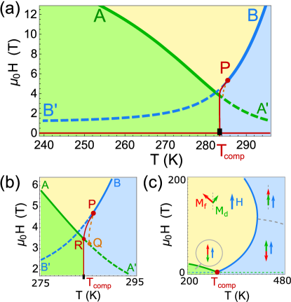
Figure 2: (a) The $H$-$T$ phase diagram near the compensation point $T_{comp}$ for GdFeCo in magnetic field directed along the easy magnetization axis. The dashed lines are the stability loss lines for the corresponding phases, solid lines correspond to the second-order phase transition, and the line $PQ$ corresponds to the stability loss of the non-collinear phase. (b) The magnified area of the $H$-$T$ phase diagram near the tricritical point $P$. (c) The qualitative zoomed out $H$-$T$ phase diagram up to magnetic fields of the order of 200 T.

Three different phases are present in the magnetic phase diagram. Figure 2 shows these phases: low-temperature collinear $\theta=0$ (green area), high-temperature collinear $\theta=\pi$ (blue area) and the non-collinear (angular) phase $\theta=\theta(H,T)$ (yellow area), which is described by Eq. (6). The collinear phase $\theta=0$ exists below $AA^{\prime}$ line, whereas the collinear phase $\theta=\pi$ exists below $BB^{\prime}$ line. These lines are the stability loss lines for the corresponding phases. The area of the angular phase is limited from below by $AQPB$-curve. The zoomed in area of the phase diagram around the point $P$ is shown in Fig. 2(b) and the zoomed out phase diagram is shown in Fig. 2(c) along with schematically drawn directions of the sublattice magnetizations in each phase. At the dashed gray line in Fig. 2(c) the condition $H_{eff}(T)=0$ is fulfilled.

There are several first- and second-order phase transitions in the vicinity of the magnetization compensation temperature $T_{comp}$. The second-order phase transitions are denoted by lines $AR$ and $PB$ and characterized by a continuous change of the order parameter across the line. The dashed lines in Fig. 2 are the lines of the stability loss and denote the theoretical temperature-dependent boundaries for the field hysteresis around the first-order phase transition at the line $H=0$. The line between $T_{comp}$ and point $P$ corresponds to another and less trivial first-order phase transition. Magnified area of the magnetic phase diagram in the vicinity of the point $P$ is shown in Fig. 2(b). The line $T_{comp}R$ corresponds to the line at which the two collinear phases phases ($\theta=0$ and $\theta=\pi$) have equal thermodynamic potentials $\Phi(0)=\Phi(\pi)$. Both phases coexist to the left and to the right from $T_{comp}R$. Above line $AR$ there is no minimum of the thermodynamic potential for the collinear phase $\theta=0$ anymore and the spins turn continuously into the non-collinear phase. At line $RP$ the first-order phase transition continues, but now it is the transition between the angular phase and the collinear $\theta=\pi$ phase. At point $P$ the order of the transition changes from first to second. According to the conventional classification, this is the tricritical point Lawrie and Sarbach (1984), in the vicinity of which many physical quantities, such as heat capacity or magnetic susceptibility, experience anomalous behavior.

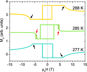
Figure 3: Dependence of the component of the $d$-sublattice magnetization along the easy axis direction on the magnetic field at different temperatures. Black and red arrows indicate second- and first-order transition points, respectively.

The first-order phase transition across $T_{comp}P$ line and the tricritical point $P$ in rare-earth ferrimagnets with similar properties were reported earlier Goransky and Zvezdin (1969); Zvezdin and Matveev (1972). However, in the previous studies it was claimed that the temperature corresponding to the tricritical point is smaller than the magnetization compensation temperature $T_{P}<T_{comp}$. The possibility for anomalous temperature dependent hysteresis loops in the vicinity of the compensation point of ferrimagnets had been overseen and it had been believed that the observed hysteresis loops are due to inhomogeneities. The relation between this previously overseen first-order phase transition and the observed hysteresis behavior is as follows. Applying an external magnetic field and measuring the magnetization behavior, one expects to observe a minor hysteresis loop corresponding to the first-order phase transition between two collinear phases $\theta=0$ and $\theta=\pi$. The coercive field of this minor hysteresis loop increases upon approaching the compensation temperature. In the temperature range between the compensation and the tricritical points ($T_{comp}<T<T_{P}$) upon an increase of the external magnetic field the compound undergoes not one, but two first-order phase transitions. First - the one, which results in a hysteresis loop around $H=0$, as explained above. Second - the spin-flop transition to the non-collinear phase, which will also result in a hysteresis at higher magnetic fields. The size of the second jump of magnetization and its hysteresis will then decrease and, subsequently, vanish at the tricritical point. Figure 3 shows the calculated magnetic field dependencies of the normal component of the $d$-sublattice magnetization at various temperatures in the vicinity of the compensation point. One can see a remarkable qualitative agreement of the calculations with anomalous temperature dependent hysteresis loops earlier observed in rare-earth transition metal alloys experimentally. Hence, here we have suggested an alternative explanation of the anomalous hysteresis loops without relying on inhomogeneities and large exchange-bias field. The observed hysteresis loops can be seen as an intrinsic property and explained in terms of first- and second-order phase transitions in the compound.

In the last decade the spin dynamics of rare-earth transition-metal alloys has been attracting an intense research interest due to the unique capability of these materials to reverse their magnetization at the record-breaking speed under action of sub-picosecond laser pulses Stanciu et al. (2007a). In the research aiming to understand the mechanisms of the ultrafast laser-induced magnetization reversal computational methods have been playing a decisive role Vahaplar et al. (2009); Ostler et al. (2012); Radu et al. (2011); Atxitia et al. (2013); Moreno et al. (2017); Chimata et al. (2015). It is clear that the value of the magnetic anisotropy of the rare-earth sublattice in ferrimagnets is an important input parameter which may greatly influence the outcome of such simulations. In GdFeCo, the rare-earth anisotropy constant may be expected to be larger than that of iron because the strength of the spin-orbit coupling depends on the nucleus charge $Z$ very close to $Z^{4}$-law (for more accurate evaluations, see Refs. Blume and Watson (1963); Blume et al. (1964)). Taking into account excited multiplets with nonzero orbital angular momentum $L$, the large single-ion anisotropy can be explained as a result of the spin-orbit coupling and the crystal field. More specifically, the large rare-earth anisotropic contribution can be calculated from microscopic theory by taking into account local crystal field of single rare-earth ion environment and spin-orbit coupling simultaneously: $\hat{V}=\sum_{i}\lambda_{SO}\hat{\bm{l}_{i}}\hat{\bm{s}_{i}}+\sum_{i}\sum_{k,q}B^{q}_{k}\hat{C}^{k}_{q}({\bm{l}_{i}})$, where $\lambda_{SO}$ is the spin-orbit coupling constant, index $i$ spans $f$-electrons of Gd³⁺ ion, $B^{q}_{k}$ are the crystal field parameters and $\hat{C}^{k}_{q}({\bm{l}_{i}})$ are the irreducible tensor operators. In perturbation theory of the third order and by taking into account states from both ground ${}^{8}S$ and excited ${}^{6}P$ terms one obtains the spin-hamiltonian with contribution of the form $D\left(S^{2}_{z}-\frac{1}{3}S(S+1)\right)$ Van Vleck and Penney (1934); Watanabe (1957); Hutchison et al. (1957). The existing estimations of $D$ from both theory and experiment Altshuler and Kozyrev (1972) are of the order of $10^{-2}-10^{-1}$ cm^-1/ion. Such a value corresponds to the large gadolinium anisotropy constant $K_{R}$ used in our calculations.

Moreover, it is expected that in compounds with rare-earth ions with non-zero orbital momentum in the ground state (Tb, Dy, Sm), the effect of the rare-earth magnetic anisotropy will be even more pronounced than in the case of Gd. For instance, in the simulations of TbCo Moreno et al. (2017) in order to mimic the experimentally observed dependence of magnetic anisotropy on concentration of Tb, it was necessary to set 10 times larger anisotropy for the Tb subllatice compared to the one of Co. Our work provides an approach for experimental verification of element-specific magnetic anisotropies in the rare-earth transition metal ferrimagnets.

IV Conclusion

In conclusion, we investigated the $H$-$T$ phase diagram for a rare-earth - transition metal ferrimagnet in the case of magnetic field directed along the easy magnetization axis. We showed that if the rare-earth anisotropy is larger than that of the $d$-sublattice, the spin-flop transition from collinear to noncollinear phase is either the first- or the second-order phase transition. Just above the compensation temperature the phase transition is of the first order. Starting from the tricritical point $P$, and at higher temperatures the spin-flop becomes a phase transition of the second order. Such a temperature dependent order of the transition from collinear to non-collinear spin phase allows us to explain anomalous hysteresis loops in rare-earth-transition metal alloys without involving the exchange bias between the surface and the bulk. Hence, we suggest that such hysteresis loops are an intrinsic property of the alloys of GdFeCo-type, which have become model materials in spintronics Dai et al. (2012), magnonics Stanciu et al. (2007b, 2006) and ultrafast magnetism Hohlfeld et al. (2001, 2009); Stanciu et al. (2007c); Graves et al. (2013). Note that at the tricritical point many response functions (heat capacity, magnetic susceptibility, etc.) experience anomalous behavior, which open totally new opportunities for fundamental and applied research of the alloys.

V Acknowledgements

This research has been supported by RSF grant No. 17-12-01333.

Appendix A Derivation of the thermodynamic potential

We start from a more general form of the Hamiltonian introduced in eq. (1) that includes exchange interaction within $f$-sublattice. This term can often be neglected due to its smallnessZvezdin et al. (1985). First, we restrict ourselves to a ground state term and use Wigner-Eckart theorem to express the spin operators $\bm{S}_{i}$ through total mechanical momentum $\bm{J}_{i}$. We obtain the components of the total Hamiltonian:

$$\begin{split}\mathcal{H}_{f,d}&=\mathcal{H}^{f,d}_{cr}-\frac{1}{2}(g_{J}^{f,d})^{2}\mu_{B}^{2}\sum_{i_{1},i_{2}\in f,d}\bm{J}_{i_{1}}T^{f,d}_{i_{1}i_{2}}\bm{J}_{i_{2}}+|g_{J}^{f,d}|\mu_{B}\bm{H}\sum_{i\in f,d}\bm{J}_{i},\\ \mathcal{H}_{f-d}&=-g_{J}^{d}g_{J}^{f}\mu_{B}^{2}\sum_{i_{1}\in f,i_{2}\in d}\bm{J}_{i_{1}}T^{f-d}_{i_{1}i_{2}}\bm{J}_{i_{2}},\end{split}$$ (7)

where exchange matrices $T_{d,f}$ and $T_{f-d}$ are linearly proportional to those of $\mathcal{J}^{d,f}$ and $\mathcal{J}^{f-d}$. We introduce an effective free energy (the thermodynamic potential of nonequilibrium state, see ref. [Zvezdin et al., 1985]) that is the function of both magnetic field and magnetizations $\bm{M}_{f,d}$:

$$\Phi=F+\bm{h}_{f}\bm{M}_{f}+\bm{h}_{d}\bm{M}_{d},$$ (8)

where

$$F=-T\ln\mathrm{Tr}\left\{\exp\left(\mathcal{H}-\bm{h}_{f}\hat{\bm{M}}_{f}-\bm{h}_{d}\hat{\bm{M}}_{d}\right)\right\}$$ (9)

is the thermodynamic free energy and the total sublattice magnetization operators are $\hat{\bm{M}}_{f,d}=g\mu_{B}\sum_{i\in f,d}\bm{J}_{i}$. The equations for the sublattice magnetizations $\bm{M}_{f,d}=-\frac{\partial F}{\partial\bm{h}_{f,d}}$ are viewed as the conditions defining the values of Lagrange multipliers $\bm{h}_{f}$ and $\bm{h}_{d}$. In the derivation, we take the trace over the ground state terms, whereas tracing for the excited states may account for a large rare-earth ion anisotropy. This question was discussed above in the paper.

Using that the intersublattice exchange energy is 2-3 orders of magnitude smaller than the exchange within the $d$ subsystem we assume the $f$-$d$ homogeneous Hisenberg exchange being equal to

$$\mathcal{H}_{f-d}=\widetilde{\mathcal{H}}_{f-d}=-\frac{1}{N_{d}}g\mu_{B}\sum_{i_{1}\in f,i_{2}\in d}\bm{J}_{i_{1}}T^{f-d}_{i_{1}i_{2}}\bm{M}_{d}$$ (10)

and treat the $d$-subsystem in the mean-field approximation Zvezdin et al. (1985). From this equation, the $f-d$ exchange coupling constant $\lambda$ can be determined.

In our approximation, the absolute value of the magnetization $\bm{M}_{d}$ is saturated by the $d$-exchange and only its direction is varying. The matrix elements of the crystal field Hamiltonian are small in comparison to both exchanges, thus we can treat it perturbatively; we also neglect the $f$-$f$ exchange. We obtain:

$$\Phi=-\bm{M}_{d}\cdot\left(\bm{H}-\bm{h}_{d}\right)+\left\langle\mathcal{H}_{cr}^{d}\right\rangle-T\ln\mathrm{Tr}_{f}\left\{\exp\left(\mathcal{H}_{f}+\widetilde{\mathcal{H}}_{f-d}-\bm{h}_{f}\hat{\bm{M}}_{f}\right)\right\}+\bm{h}_{f}\bm{M}_{f},$$ (11)

where $\mathrm{Tr}_{f}$ denotes the trace over the $f$-subsystem ground state term states. This is a quite general result that allows for a high accuracy treatment of $f$-$d$ magnets. For subsequent consideration we simplify this expression further. For a GdFeCo-like alloy the single-ion crystal field for both sublattices may be represented by its first term of expansion $\left(\mathcal{H}^{f,d}_{cr}\right)_{i}=\left(A^{2}_{0}\right)_{i}\sum_{j}C^{0}_{2}(\bm{l}_{j})$, where $C^{n}_{m}$ are the Steven’s operators Abragam and Bleaney (2012) and $\bm{l}_{j}$ is the angular momentum of $j$-th electron belonging to $i$-th ion. According to Wigher-Eckart theorem if we restrain our consideration to the ground state term with given $J$, the result can be represented as a function of total angular momentum of the ion: $\left(\mathcal{H}^{f,d}_{cr}\right)_{i}=\left(B^{2}_{0}\right)_{i}Y^{0}_{2}(\bm{J}_{i})$. When viewing the crystal field as a perturbation, we introduce the quantization axis along the external field and find $d$-sublattice $\left\langle\mathcal{H}^{d}_{cr}\right\rangle=-4/3\sqrt{\pi/5}K_{d}Y^{0}_{2}(\bm{M}_{d}/M_{d})$ Abragam and Bleaney (2012), where $Y^{0}_{2}$ are the spherical harmonics and we have introduced the uniaxial magnetocrystalline anisotropy $K_{d}$.

Treating the crystal field acting on $f$ ions as perturbation (similarly to $d$-crystal field), we also assume the magnetization $\bm{M}_{f}$ to be aligned with the effective magnetic field acting on it and release the Lagrangian multiplier $\bm{h}_{f}$, obtaining the Brillouin function for after tracing the third term in expression (11): $M_{f}\approx gJ_{f}\mu_{B}N_{f}B_{J}\left(\frac{gJ_{f}\mu_{B}{H}_{eff}}{kT}\right)$, where $\bm{H}_{eff}=\bm{H}-\lambda\bm{M}_{d}$ and the $f$-$d$ exchange coupling constant $\lambda=\mathcal{J}$. The total angular momentum eigenvalue $J_{f}$ for the ground state term ${}^{8}S$ of Gd ions is equal to 7/2. Finally, we arrive at the thermodynamic potential in the form given by eq. (3).

References

- Buschow (1977) K. Buschow, Rep. Prog. Phys. 40, 1179 (1977).
- Franse and Radwański (1993) J. Franse and R. Radwański, Handbook of Magnetic Materials 7, 307 (1993).
- Belov et al. (1976) K. P. Belov, A. K. Zvezdin, A. M. Kadomtseva, and R. Levitin, Sov. Phys. Usp. 19, 574 (1976).
- Duc et al. (2002) N. Duc, D. K. Anh, and P. Brommer, Physica B: Condensed Matter 319, 1 (2002).
- Sechovskỳ et al. (1994) V. Sechovskỳ, L. Havela, K. Prokeš, H. Nakotte, F. De Boer, and E. Brück, J. Appl. Phys. 76, 6913 (1994).
- Žutić et al. (2004) I. Žutić, J. Fabian, and S. Das Sarma, Rev. Mod. Phys. 76, 323 (2004).
- Kruglyak et al. (2010) V. Kruglyak, S. Demokritov, and D. Grundler, Journal of Physics D: Applied Physics 43, 264001 (2010).
- Stanciu et al. (2007a) C. D. Stanciu, F. Hansteen, A. V. Kimel, A. Kirilyuk, A. Tsukamoto, A. Itoh, and T. Rasing, Phys. Rev. Lett. 99, 047601 (2007a).
- Vahaplar et al. (2009) K. Vahaplar, A. M. Kalashnikova, A. V. Kimel, D. Hinzke, U. Nowak, R. Chantrell, A. Tsukamoto, A. Itoh, A. Kirilyuk, and T. Rasing, Phys. Rev. Lett. 103, 117201 (2009).
- Moser et al. (2002) A. Moser, K. Takano, D. T. Margulies, M. Albrecht, Y. Sonobe, Y. Ikeda, S. Sun, and E. E. Fullerton, Journal of Physics D: Applied Physics 35, R157 (2002).
- Ostler et al. (2012) T. Ostler, J. Barker, R. Evans, R. Chantrell, U. Atxitia, O. Chubykalo-Fesenko, S. El Moussaoui, L. Le Guyader, E. Mengotti, L. Heyderman, et al., Nature communications 3 (2012), 10.1038/ncomms1666.
- Khorsand et al. (2012) A. R. Khorsand, M. Savoini, A. Kirilyuk, A. V. Kimel, A. Tsukamoto, A. Itoh, and T. Rasing, Phys. Rev. Lett. 108, 127205 (2012).
- Radu et al. (2011) I. Radu, K. Vahaplar, C. Stamm, T. Kachel, N. Pontius, H. Dürr, T. Ostler, J. Barker, R. Evans, R. Chantrell, et al., Nature 472, 205 (2011).
- Graves et al. (2013) C. Graves, A. Reid, T. Wang, B. Wu, S. De Jong, K. Vahaplar, I. Radu, D. Bernstein, M. Messerschmidt, L. Müller, et al., Nature materials 12, 293 (2013).
- Stanciu et al. (2007b) C. D. Stanciu, F. Hansteen, A. V. Kimel, A. Tsukamoto, A. Itoh, A. Kirilyuk, and T. Rasing, Phys. Rev. Lett. 98, 207401 (2007b).
- Le Guyader et al. (2012) L. Le Guyader, S. El Moussaoui, M. Buzzi, R. Chopdekar, L. Heyderman, A. Tsukamoto, A. Itoh, A. Kirilyuk, T. Rasing, A. Kimel, et al., App. Phys. Lett. 101, 022410 (2012).
- Xu et al. (2010) C. Xu, Z. Chen, D. Chen, S. Zhou, and T. Lai, Applied Physics Letters 96, 092514 (2010), https://doi.org/10.1063/1.3339878 .
- Taylor and Gangulee (1980) R. C. Taylor and A. Gangulee, Phys. Rev. B 22, 1320 (1980).
- Esho (1976) S. Esho, Japanese Journal of Applied Physics 15, 93 (1976).
- Chen and Malmhäll (1983) T. Chen and R. Malmhäll, Journal of Magnetism and Magnetic Materials 35, 269 (1983).
- Okamoto and Miura (1989) K. Okamoto and N. Miura, Physica B: Condensed Matter 155, 259 (1989).
- Becker et al. (2017) J. Becker, A. Tsukamoto, A. Kirilyuk, J. C. Maan, T. Rasing, P. C. M. Christianen, and A. V. Kimel, Phys. Rev. Lett. 118, 117203 (2017).
- Amatsu et al. (1977) M. Amatsu, S. Honda, and T. Kusuda, IEEE Trans. Magn. 13, 1612 (1977).
- Chen et al. (2015) K. Chen, D. Lott, F. Radu, F. Choueikani, E. Otero, and P. Ohresser, Scientific reports 5 (2015), 10.1038/srep18377.
- Goransky and Zvezdin (1969) B. Goransky and A. Zvezdin, JETP Lett. 10, 196 (1969).
- Zvezdin and Matveev (1972) A. Zvezdin and V. Matveev, JETP 35, 140 (1972).
- Zvezdin (1995) A. Zvezdin, Handbook of Magnetic Materials 9, 405 (1995).
- Sabdenov et al. (2017a) C. K. Sabdenov, M. Davydova, K. Zvezdin, A. Zvezdin, A. Andreev, D. Gorbunov, E. Tereshina, Y. Skourski, J. Šebek, and I. Tereshina, Journal of Alloys and Compounds 708, 1161 (2017a).
- Sabdenov et al. (2017b) C. K. Sabdenov, M. Davydova, K. Zvezdin, D. Gorbunov, I. Tereshina, A. Andreev, and A. Zvezdin, J. Low. Temp. Phys 43, 551 (2017b).
- Zvezdin et al. (1985) A. Zvezdin, V. Matveev, A. Mukhin, and A. Popov, Moscow Izdatel Nauka (1985).
- Abragam and Bleaney (2012) A. Abragam and B. Bleaney, Electron paramagnetic resonance of transition ions (OUP Oxford, 2012).
- Lawrie and Sarbach (1984) I. D. Lawrie and S. Sarbach, Phase transitions and critical phenomena, Vol. 9 (Academic, London, 1984) pp. 1–161.
- Atxitia et al. (2013) U. Atxitia, T. Ostler, J. Barker, R. F. L. Evans, R. W. Chantrell, and O. Chubykalo-Fesenko, Phys. Rev. B 87, 224417 (2013).
- Moreno et al. (2017) R. Moreno, T. A. Ostler, R. W. Chantrell, and O. Chubykalo-Fesenko, Phys. Rev. B 96, 014409 (2017).
- Chimata et al. (2015) R. Chimata, L. Isaeva, K. Kádas, A. Bergman, B. Sanyal, J. H. Mentink, M. I. Katsnelson, T. Rasing, A. Kirilyuk, A. Kimel, O. Eriksson, and M. Pereiro, Phys. Rev. B 92, 094411 (2015).
- Blume and Watson (1963) M. Blume and R. Watson, in Proc. R. Soc. Lond. A, Vol. 271 (The Royal Society, 1963) pp. 565–578.
- Blume et al. (1964) M. Blume, A. J. Freeman, and R. E. Watson, Phys. Rev. 134, A320 (1964).
- Van Vleck and Penney (1934) J. Van Vleck and W. Penney, The London, Edinburgh, and Dublin Philosophical Magazine and Journal of Science 17, 961 (1934).
- Watanabe (1957) H. Watanabe, Progress of Theoretical Physics 18, 405 (1957).
- Hutchison et al. (1957) C. Hutchison, B. Judd, and D. Pope, Proceedings of the Physical Society. Section B 70, 514 (1957).
- Altshuler and Kozyrev (1972) S. A. Altshuler and B. M. Kozyrev, Electron paramagnetic resonance of compounds of elements of intermediate groups (Nauka, 1972).
- Dai et al. (2012) B. Dai, T. Kato, S. Iwata, and S. Tsunashima, IEEE Trans. Magn. 48, 3223 (2012).
- Stanciu et al. (2006) C. D. Stanciu, A. V. Kimel, F. Hansteen, A. Tsukamoto, A. Itoh, A. Kirilyuk, and T. Rasing, Phys. Rev. B 73, 220402 (2006).
- Hohlfeld et al. (2001) J. Hohlfeld, T. Gerrits, M. Bilderbeek, T. Rasing, H. Awano, and N. Ohta, Phys. Rev. B 65, 012413 (2001).
- Hohlfeld et al. (2009) J. Hohlfeld, C. D. Stanciu, and A. Rebei, Appl. Phys. Lett. 94, 152504 (2009).
- Stanciu et al. (2007c) C. D. Stanciu, A. Tsukamoto, A. V. Kimel, F. Hansteen, A. Kirilyuk, A. Itoh, and T. Rasing, Phys. Rev. Lett. 99, 217204 (2007c).