Truly Proximal Policy Optimization

Abstract

Proximal policy optimization (PPO) is one of the most successful deep reinforcement-learning methods, achieving state-of-the-art performance across a wide range of challenging tasks. However, its optimization behavior is still far from being fully understood. In this paper, we show that PPO could neither strictly restrict the likelihood ratio as it attempts to do nor enforce a well-defined trust region constraint, which means that it may still suffer from the risk of performance instability. To address this issue, we present an enhanced PPO method, named Truly PPO. Two critical improvements are made in our method: 1) it adopts a new clipping function to support a rollback behavior to restrict the difference between the new policy and the old one; 2) the triggering condition for clipping is replaced with a trust region-based one, such that optimizing the resulted surrogate objective function provides guaranteed monotonic improvement of the ultimate policy performance. It seems, by adhering more truly to making the algorithm proximal — confining the policy within the trust region, the new algorithm improves the original PPO on both sample efficiency and performance.

Keywords: proximal policy optimization, trust region policy optimization, policy constraint, policy metric, policy gradient

1 Introduction

Deep model-free reinforcement learning has achieved great successes in recent years, notably in video games (Mnih et al., 2015), board games (Silver et al., 2017), robotics (Levine et al., 2016; Liu et al., 2018), and challenging control tasks (Schulman et al., 2016; Rai et al., 2019). Policy gradient (PG) methods are useful model-free policy search algorithms, updating the policy with an estimator of the gradient of the expected return (Peters and Schaal, 2008; Hu et al., 2019). One major challenge of PG-based methods is to estimate the right step size for the policy updating, and an improper step size may result in severe policy degradation due to the fact that the input data strongly depends on the current policy (Kakade and Langford, 2002; Schulman et al., 2015). For this reason, the trade-off between learning stability and learning speed is an essential issue to be considered for a PG method.

The well-known trust region policy optimization (TRPO) method addressed this problem by imposing onto the objective function a trust region constraint so as to control the KL divergence between the old policy and the new one (Schulman et al., 2015). This can be theoretically justified by showing that optimizing the policy within the trust region leads to guaranteed monotonic performance improvement. However, the complicated second-order optimization involved in TRPO makes it computationally inefficient and difficult to scale up for large scale problems when extending to complex network architectures. Proximal Policy Optimization (PPO) significantly reduces the complexity by adopting a clipping mechanism so as to avoid imposing the hard constraint completely, allowing it to use a first-order optimizer like the Gradient Descent method to optimize the objective (Schulman et al., 2017). As for the mechanism for dealing with the learning stability issue, in contrast with the trust region method of TRPO, PPO tries to remove the incentive for pushing the policy away from the old one when the likelihood ratio between them is out of a clipping range. PPO is proven to be very effective in dealing with a wide range of challenging tasks, while being simple to implement and tune.

However, despite its success, the actual optimization behavior of PPO is less studied, highlighting the need to study the “proximal” property of PPO. Some researchers have raised concerns about whether PPO could restrict the likelihood ratio as it attempts to do (Wang et al., 2019b; Ilyas et al., 2018), and since there exists an obvious gap between the heuristic likelihood ratio constraint and the theoretically justified trust region constraint, it is natural to ask whether PPO enforces a trust region-like constraint as well to ensure its stability in learning?

In this paper, we formally address both the above questions and give negative answers to both of them. In particular, we found that PPO could neither strictly restrict the likelihood ratio nor enforce a trust region constraint. The former issue is mainly caused by the fact that PPO could not entirely remove the incentive for pushing the policy away, while the latter is mainly due to the inherent difference between the two types of constraints adopted by PPO and TRPO respectively.

Inspired by the insights above, we propose an enhanced PPO method, named Truly PPO. In particular, we apply a negative incentive to prevent the policy from being pushed away during training, which we called a rollback operation. Furthermore, we replace the triggering condition for clipping with a trust region-based one, such that optimizing the resulting surrogate objective function provides guaranteed monotonic improvement of the ultimate policy performance. Truly PPO actually combines the strengths of TRPO and PPO — it is theoretically justified and is simple to implement with first-order optimization. Extensive results on several benchmark tasks show that the proposed methods significantly improve both the policy performance and the sample efficiency. Source code is available at https://github.com/wangyuhuix/TrulyPPO.

A preliminary version of this work appears in (Wang et al., 2019a). This expanded version aims to provide more in-depth investigations of the characteristics of the proposed methods. Specifically, we propose a new objective function combining trust region-based clipping with rollback operation on KL divergence. We show that it owns a better theoretical characteristic of the monotonic improvement and performs much better in practice. Moreover, the detailed proofs of the theorems and more derivation details are included to provide a more detailed description of the theoretical properties. More experiments and comparison with the state-of-art methods have been added to show the effectiveness of the proposed methods. Last but not least, we give an elaborate summary of the relation with prior works on constraining policy and show how could our finds guide future research.

In what follows, we first introduce the preliminaries of proximal policy optimization in Section 2, then we give an analysis of the “proximal” property of PPO in Section 3. Next, we propose three variants of PPO to enhance its ability in restricting policy in Section 4. We give a detailed relation with prior works in Section 5. The main experimental results are given in Section 6, and the paper is concluded in Section 7.

2 Preliminaries

A Markov Decision Processes (MDP) is described by the tuple $(\mathcal{S},\mathcal{A},{\cal T},c,\rho_{1},\gamma)$. $\mathcal{S}$ and $\mathcal{A}$ are the state space and action space; ${\cal T}:\mathcal{S}\times\mathcal{A}\times\mathcal{S}\rightarrow{\mathbb{R}}$ is the transition probability distribution; $c:\mathcal{S}\times\mathcal{A}\rightarrow\mathbb{R}$ is the reward function; $\rho_{1}$ is the distribution of the initial state $s_{1}$, and $\gamma\in(0,1)$ is the discount factor. The performance of a policy $\pi$ is defined as $\eta(\pi)={\mathbb{E}_{s\sim{\rho^{\pi}},a\sim\pi}}\left[{c(s,a)}\right]$ where ${\rho^{{\pi}}}(s)=(1-\gamma)\mathop{\sum}_{t=1}^{\infty}{\gamma^{t-1}}{\rho_{t}^{{\pi}}}(s)$, $\rho_{t}^{\pi}$ is the density function of state at time $t$.

Policy gradients methods (Sutton et al., 1999) update the policy by the following surrogate performance objective,

$$L^{\rm PG}_{\pi_{\rm old}}(\pi)={{\mathbb{E}_{s,a}}\left[{\ratio[s,a][\pi][\pi_{\rm old}]A_{s,a}^{\pi_{\rm old}}}\right]+\eta(\pi_{\rm old})}$$ (1)

where $\ratio[s,a][\pi][\pi_{\rm old}]={\pi(a|s)}/{\pi_{\rm old}(a|s)}$ is the likelihood ratio between the new policy $\pi$ and the old policy $\pi_{\rm old}$, $A_{s,a}^{\pi_{\rm old}}\triangleq\mathbb{E}[R_{t}^{\gamma}|s_{t}=s,a_{t}=a;\pi_{\rm old}]-\mathbb{E}[R_{t}^{\gamma}|s_{t}=s;\pi_{\rm old}]$ is the advantage value function of the old policy $\pi_{\rm old}$. For simplicity, we will omit writing superscript/subscript $\pi_{\rm old}$ explicitly, e.g., $L^{\rm PG}(\pi),\ratio[s,a][\pi],A_{s,a}$.

In practical deep RL algorithms, the policy are usually parametrized by Deep Neural Networks (DNNs). For discrete action space tasks where $|{\cal A}|=D$, the policy is parametrized by $\pi_{\theta}(s_{t})=f^{p}_{\theta}(s_{t})$, where $f^{p}_{\theta}$ is the DNN outputting a vector which represents a $D$-dimensional discrete distribution. For continuous action space tasks, it is standard to represent the policy by a Gaussian policy, i.e., $\pi_{\theta}(a|s_{t})=\mathcal{N}(a|f^{\mu}_{\theta}(s_{t}),f^{\Sigma}_{\theta}(s_{t}))$ (Williams, 1992; Mnih et al., 2016), where $f^{\mu}_{\theta}$ and $f^{\Sigma}_{\theta}$ are the DNNs which output the mean and the covariance matrix of the Gaussian distribution.

2.1 Trust Region Policy Optimization

The well-known Trust Region Policy Optimization (TRPO) is derived the following performance bound:

Theorem 1

Let

$C=\mathop{\max}\limits_{s,a}\left|{{A_{s,a}}}\right|{4\gamma}/{{{(1-\gamma)}^{2}}}$, $D_{{\rm{KL}}}^{{s}}\left({\pi_{\rm old},\pi}\right)\triangleq D_{{\rm{KL}}}\left({\pi_{\rm old}(\cdot|s)||\pi(\cdot|s)}\right)$, ${M}(\pi)={L^{\rm PG}}(\pi)-C\max_{s\in{\cal S}}D_{\rm{KL}}^{\rm{s}}\left({\pi_{\rm old},\pi}\right).$ We have

$$\eta(\pi)\geq{M}(\pi),\eta(\pi_{\rm old})={M}(\pi_{\rm old}).$$ (2)

This theorem implies that maximizing ${M}(\pi)$ guarantee non-decreasing of the performance of the new policy $\pi$. TRPO imposed a constraint on the KL divergence:

$$\mathop{\max}\limits_{\pi} L^{\rm PG}(\pi)$$ (3a)

s.t. $$\max_{s\in{\cal S}}D_{\rm{KL}}^{\rm{s}}\left({\pi_{\rm old},\pi}\right)\leq\delta$$ (3b)

Constraint (3b) is called the trust region-based constraint, which is a constraint on the KL divergence between the old policy and the new one.

2.2 Proximal Policy Optimization

Proximal policy optimization (PPO) attempts to restrict the policy by a clipping function (Schulman et al., 2017).

$$L^{\rm{{\rm CLIP}}}(\pi)=\mathbb{E}\left[\min\left(\ratio[s,a][\pi]A_{s,a},{{\cal F}^{\rm{\rm CLIP}}}\left({\ratio[s,a][\pi],\epsilon}\right)A_{s,a}\right)\right]$$ (4)

where ${\cal F}^{\rm{\rm CLIP}}$ is defined as

$${\cal F}^{\rm{\rm CLIP}}({\ratio[s,a][\pi],\epsilon})=\begin{cases}1-\epsilon&\ratio[s,a][\pi]\leq 1-\epsilon\\ 1+\epsilon&\ratio[s,a][\pi]\geq 1+\epsilon\\ \ratio[s,a][\pi]&\text{otherwise}\end{cases}$$ (5)

where $(1-\epsilon,1+\epsilon)$ is called the clipping range, $0<\epsilon<1$ is the parameter.

Given $s_{t}\sim{\rho^{\pi_{\theta_{\rm old}}}},a_{t}\sim{\pi_{\theta_{\rm old}}}(\cdot|s_{t})$, which are sampled using the parametrized policy $\pi_{\theta_{\rm old}}$. For simplicity, we will use subscript $t$ to denote the corresponding value for sample $(s_{t},a_{t})$, e.g., $\ratio[t][\pi_{\theta}]\triangleq\ratio[s_{t},a_{t}][\pi_{\theta}]$, $A_{t}\triangleq A_{s_{t},a_{t}}$; and we will also use functions of $\theta$ and the ones of $\pi$ alternatively, e.g., $\ratio[t][\theta]\triangleq\ratio[t][\pi_{\theta}]$, $L^{\rm{CLIP}}(\theta)\triangleq L^{\rm{CLIP}}(\pi_{\theta})$ and $D_{\rm KL}^{s}(\theta_{\rm old},\theta)\triangleq D_{\rm KL}^{s}(\pi_{\theta_{\rm old}},\pi_{\theta})$. The overall empirical objective function of data $\{s_{t},a_{t},A_{t}\}_{t=1}^{T}$ is $\hat{L}^{\rm{{\rm CLIP}}}(\theta)$. To provide a more intuitive form on how the clipping function works, the objective function for a single sample $(s_{t},a_{t})$ can be rewritten in the following form:

$$[left={L^{\rm{{\rm CLIP}}}_{t}(\theta)=\empheqlbrace} {(1-\epsilon)}A_{t}$$ (6a)

$${(1+\epsilon)}A_{t}$$ (6b)

$$r_{t}(\theta)A_{t}$$ otherwise

The case (6a) and (6b) are called the clipping condition. As the equation implies, once $r_{t}(\theta)$ is out of the clipping range (with a certain condition of $A_{t}$), the gradient of $L^{\rm{{\rm CLIP}}}_{t}(\theta)$ w.r.t. $\theta$ will be zero. As a result, $\ratio[t][\theta]$ could stop moving outward and the policy could be restricted.

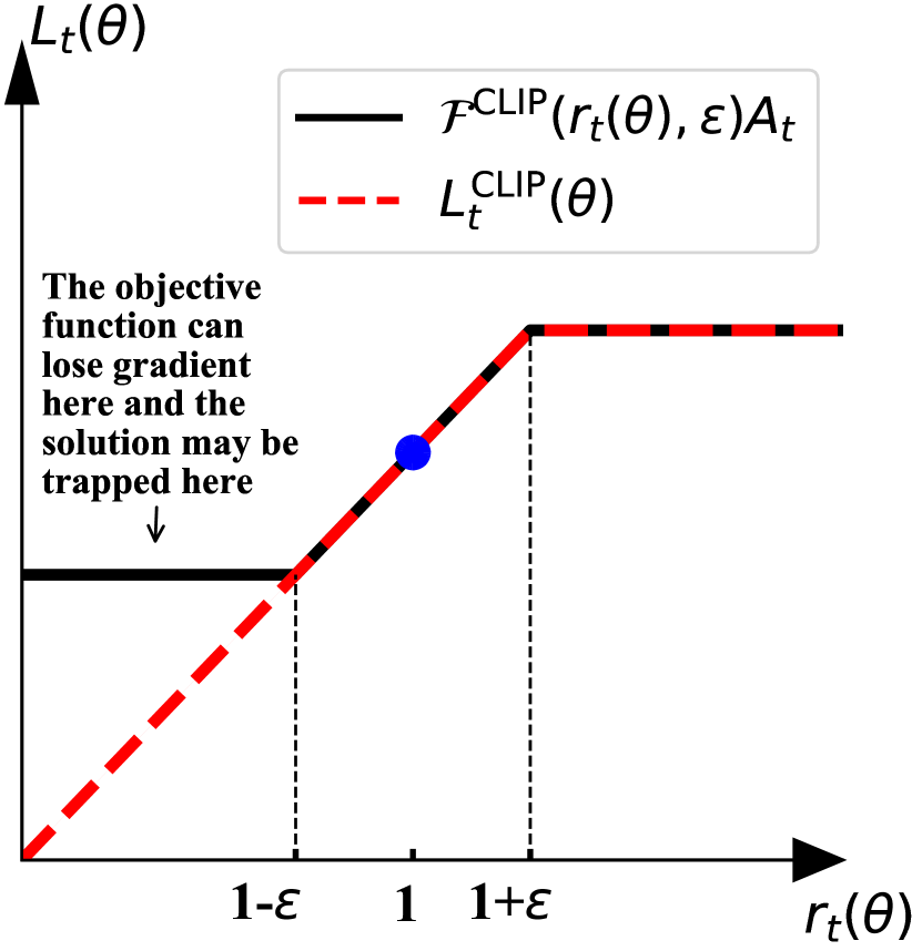
(a) $A_{t}>0$

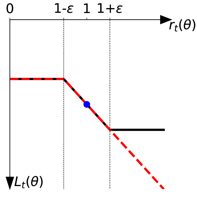
(b) $A_{t}<0$

Figure 1: Plots showing the surrogate function as functions of the likelihood ratio $\ratio[t][\theta]$ for positive advantages (left) and negative advantages (right). For the one without the minimum operation (black solid line), i.e., ${\cal F}^{\rm{\rm CLIP}}({r_{t}(\theta),\epsilon})A_{t}$, it can lose gradient for improving $\ratio[t][\theta]$ once $|\ratio[t][\theta]-1|>\epsilon$, even the $\ratio[t][\theta]$ is not improved ($\ratio[t][\theta]<1-\epsilon$ when $A_{t}<0$ or $\ratio[t][\theta]>1+\epsilon$ when $A_{t}<0$). While the one with the minimum operation (red dashed line), i.e., $L^{\rm{CLIP}}_{t}(\theta)$, does not suffer from this issue.

The minimum between the clipped and unclipped objective in eq. 4 is designed to make the final objective $L^{\rm{CLIP}}(\theta)$ to be a lower bound on the unclipped objective (Schulman et al., 2017). It should also be noted that such operation is important for optimization, which is not referred to by prior literature. As implied in eq. 5, the clipped objective without minimum operation, i.e., ${\cal F}^{\rm CLIP}({r_{t}(\theta),\epsilon})A_{t}$, would lose gradient for improving the ratio $\ratio[t][\theta]$ once the ratio goes past the clipping range, even the objective value is worse than the initial one, i.e., $r_{t}(\theta)A_{t}<r_{t}(\theta_{old})A_{t}$. The minimum operation actually provides a remedy for this issue. To see this, eq. 6 is rewritten as

$$[left={L^{\rm{CLIP}}_{t}(\theta)=\empheqlbrace}]$$ const (6ga)

$$r_{t}(\theta)A_{t}$$ otherwise

Condition (6a) combined with (6b) is equivalent to condition (6ga). As can be seen, the ratio $\ratio[t][\theta]$ is clipped only if the objective value is improved $r_{t}(\theta)A_{t}\geq r_{t}(\theta_{{}_{\rm old}})A_{t}$ . Figure 1 depicts the mechanism of the minimum operation. We also experimented with the direct-clipping method, i.e., ${\cal F}^{\rm{\rm CLIP}}({r_{t}(\theta),\epsilon})A_{t}$, and found it performs extremely bad in practice. See Section 6.5 for more detail.

3 Analysis of the “Proximal” Property of PPO

PPO attempts to restrict the policy by clipping the likelihood ratio between the new policy and the old one. Recently, researchers have raised concerns about whether this clipping mechanism can really restrict the policy (Wang et al., 2019b; Ilyas et al., 2018). We investigate the following questions of PPO. The first one is that whether PPO could bound the likelihood ratio as it attempts to do. The second one is that whether PPO could enforce a well-defined trust region constraint, which is primarily concerned since that it is a theoretical indicator on the performance guarantee (see eq. 2) (Schulman et al., 2015). We give an elaborate analysis of PPO to answer these two questions.

Question 1

Could PPO bound the likelihood ratio within the clipping range as it attempts to do?

In general, PPO could generate an effect of preventing the likelihood ratio from exceeding the clipping range too much, but it could not strictly bound the likelihood ratio.

As we have discussed in Sec 2.2, the gradient of $L^{\rm{{\rm CLIP}}}_{t}(\theta)$ w.r.t. $\theta$ will be zero only if $r_{t}(\theta)$ is out of the clipping range. As a result, the incentive, deriving from $L^{\rm{{\rm CLIP}}}_{t}(\theta)$, for driving $r_{t}(\theta)$ to go farther beyond the clipping range is removed.

However, in practice the likelihood ratios are known to be not bounded within the clipping range (Ilyas et al., 2018). The likelihood ratios are larger than 4. on almost all the tasks, which are much larger than the upper clipping range 1.2 ($\epsilon=0.2$, see our empirical results in Section 6). One main factor for this problem is that the clipping mechanism could not entirely remove incentive deriving from the overall objective $\hat{L}^{\rm{{\rm CLIP}}}(\theta)$, which possibly push these out-of-the-range $r_{t}(\theta)$ to go farther beyond the clipping range. We formally describe this claim as follows.

Theorem 2

Given $\theta_{0}$ that $r_{t}(\theta_{0})$ satisfies the clipping condition (either condition 6a or 6b). Let $\nabla\hat{L}^{\rm{{\rm CLIP}}}(\theta_{0})$ denote the gradient of $\hat{L}^{\rm{{\rm CLIP}}}$ at $\theta_{0}$, and similarly $\nabla r_{t}(\theta_{0})$. Let $\theta_{1}=\theta_{0}+\beta\nabla\hat{L}^{\rm{{\rm CLIP}}}(\theta_{0})$, where $\beta$ is the step size. If

$$\langle\nabla\hat{L}^{\rm{{\rm CLIP}}}(\theta_{0}),\nabla r_{t}(\theta_{0})\rangle A_{t}>0$$ (6h)

then there exists some $\bar{\beta}>0$ such that for any $\beta\in(0,\bar{\beta})$, we have

$$\left|r_{t}({\theta_{1}})-1\right|>\left|r_{t}({\theta_{0}})-1\right|>\epsilon.$$ (6i)

Proof  Consider $\phi(\beta)=r_{t}(\theta_{0}+\beta\nabla\hat{L}^{\rm{{\rm CLIP}}}(\theta_{0}))$.

By chain rule, we have

$$\phi^{\prime}(0)=\langle\nabla\hat{L}^{\rm{{\rm CLIP}}}(\theta_{0}),\nabla r_{t}(\theta_{0})\rangle$$

For the case where $r_{t}(\theta_{0})\geq 1+\epsilon$ and $A_{t}>0$, we have $\phi^{\prime}(0)>0$. Hence, there exists $\bar{\beta}>0$ such that for any $\beta\in(0,\bar{\beta})$

$$\phi(\beta)>\phi(0)$$

Thus, we have

$$r_{t}(\theta_{1})>r_{t}(\theta_{0})\geq 1+\epsilon$$

We obtain

$$|r_{t}(\theta_{1})-1|>|r_{t}(\theta_{0})-1|$$

Similarly, for the case where $r_{t}(\theta_{0})\leq 1-\epsilon$ and $A_{t}<0$, we also have $|r_{t}(\theta_{1})-1|>|r_{t}(\theta_{0})-1|$.  

As this theorem implies, even the likelihood ratio $r_{t}(\theta_{0})$ is already out of the clipping range, it could be driven to go farther beyond the range (see eq. 6i). The condition (6h) requires the gradient of the overall objective $\hat{L}^{\rm{{\rm CLIP}}}(\theta_{0})$ to be similar in direction to that of $r_{t}(\theta_{0})A_{t}$. This condition possibly happens due to the similar gradients of different samples or optimization tricks. In addition, the Momentum optimization methods preserve the gradients attained before, which could possibly make this situation happen. Such condition occurs quite often in practice. We made statistics over 1 million samples on benchmark tasks in Section 6, and the condition occurs at a percentage from 25% to 45% across different tasks.

Question 2

Could PPO enforce a trust region constraint?

PPO does not explicitly attempt to impose a trust region constraint, i.e., the KL divergence between the old policy and the new one. Nevertheless, our previous work revealed that a different scale of the clipping range can affect the scale of the KL divergence (Wang et al., 2019b). Under state-action $(s_{t},a_{t})$, if the likelihood ratio $r_{t}(\theta)$ is not bounded, then neither could the corresponding KL divergence $D_{\rm KL}^{s_{t}}(\theta{{}_{\rm old}},\theta)$ be bounded. Thus, together with the previous conclusion in Question 1, we can know that PPO could not bound KL divergence. In fact, even the likelihood ratio $r_{t}(\theta)$ is bounded, the corresponding KL divergence $D_{\rm KL}^{s_{t}}(\theta{{}_{\rm old}},\theta)$ is not necessarily bounded. Formally, we have the following theorem.

Theorem 3

Assume that for discrete action space tasks where $|{\cal A}|\geq 3$, the policy is parametrized by $\pi_{\theta}(s_{t})=p_{t}\in{\mathbb{R}}^{+|{\cal A}|}$, where $\sum_{d}^{|{\cal A}|}p^{(d)}_{t}=1$; for continuous action space tasks, the policy is parametrized by $\pi_{\theta}(a|s_{t})=\mathcal{N}(a|\mu_{t},\Sigma_{t})$. Let $\Theta=\{\theta|1-\epsilon\leq r_{t}(\theta)\leq 1+\epsilon\}$. We have $\max_{\theta\in\Theta}D_{\rm KL}^{s_{t}}(\theta{{}_{\rm old}},\theta)=+\infty$ for both discrete and continuous action space tasks.

Proof  The problem $\max_{\theta\in\Theta}D_{\rm KL}^{s_{t}}(\theta{{}_{\rm old}},\theta)$ is formalized as

$$\max_{\theta} D_{\rm KL}^{s_{t}}(\theta{{}_{\rm old}},\theta)$$ (6j)

$$s.t. 1-\epsilon\leq r_{t}(\theta)\leq 1+\epsilon$$

We first prove the discrete action space case, where the problem can be transformed into the following form,

$$\max_{p} \sum_{d}p_{\rm old}^{(d)}\log\frac{p_{\rm old}^{(d)}}{p^{(d)}}$$ (6k)

$$s.t. 1-\epsilon\leq\frac{p^{(a_{t})}}{p_{\rm old}^{(a_{t})}}\leq 1+\epsilon$$

$$\sum_{d}{p^{(d)}}=1$$

where $p_{\rm old}=f^{p}_{\theta_{\rm old}}(s_{t})$. We could construct a $p_{\rm new}$ satisfies 1) $p_{\rm new}^{(d^{\prime})}=0$ for a $d^{\prime}\neq a_{t}$ where $p_{\rm old}^{(d^{\prime})}>0$; 2) $1-\epsilon\leq\frac{p^{(a_{t})}_{\rm new}}{p_{\rm old}^{(a_{t})}}\leq 1+\epsilon$. Thus we have

$$\sum_{d}p_{\rm old}^{(d)}\log\frac{p_{\rm old}^{(d)}}{p_{\rm new}^{(d)}}=+\infty$$

Then we prove the continuous action space case where $dim({\cal A})=1$. The problem (6k) can be transformed into the following form,

$$\max_{\mu,\sigma} F(\mu,\sigma)=\frac{1}{2}{\left[{-2\log\frac{\sigma}{\sigma{{}_{\rm old}}}+\frac{\sigma}{\sigma{{}_{\rm old}}}+{(\mu-\mu_{\rm old})^{2}}\sigma_{\rm old}^{-1}-1}\right]}$$ (6l)

$$s.t. 1-\epsilon\leq\frac{{\cal N}(a_{t}|\mu,\sigma)}{{\cal N}(a_{t}|\mu_{\rm old},\sigma_{\rm old})}\leq 1+\epsilon$$

where $\mu_{\rm old}=f^{\mu}_{\theta_{\rm old}}(s_{t})$, $\sigma_{\rm old}=f^{\Sigma}_{\theta_{\rm old}}(s_{t})$,

$${{\cal N}(a|\mu,\sigma)}=\frac{1}{\sqrt{2\pi}\sigma}\exp{\left(-\frac{(\mu-a)^{2}}{2\sigma^{2}}\right)}$$

As can be seen, $\lim_{\sigma\rightarrow 0}F(\mu,\sigma)=+\infty$, we just need to prove that given any $\sigma_{\rm new}<\sigma_{\rm old}$, there exists $\mu_{\rm new}$ such that

$${{\cal N}(a_{t}|\mu_{\rm new},\sigma_{\rm new})}={{\cal N}(a_{t}|\mu_{\rm old},\sigma_{\rm old})}$$

In fact, if $\sigma_{\rm new}<\sigma_{\rm old}$, then $\max_{a}{{\cal N}(a|\mu_{\rm new},\sigma_{\rm new})}>\max_{a}{{\cal N}(a|\mu_{\rm old},\sigma_{\rm old})}$ for any $\mu_{\rm new}$. Thus given any $\sigma_{\rm new}<\sigma_{\rm old}$, there always exists $\mu_{\rm new}$ such that ${{\cal N}(a_{t}|\mu_{\rm new},\sigma_{\rm new})}={{\cal N}(a_{t}|\mu_{\rm old},\sigma_{\rm old})}$.

Similarly, for the case where $dim({\cal A})>1$, we also have $\max_{\theta\in\Theta}D_{\rm KL}^{s_{t}}(\theta{{}_{\rm old}},\theta)=+\infty$.  

           

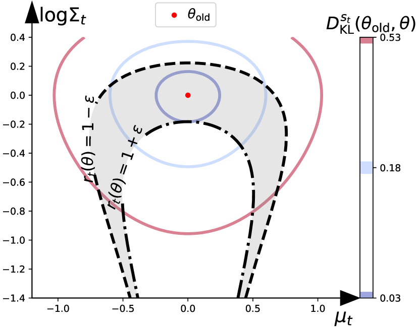
(a) Case in Continuous Action Space

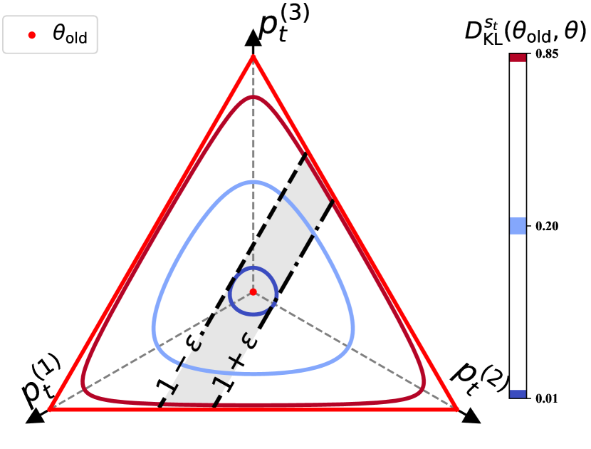
(b) Case in Discrete Action Space

Figure 2: The grey area shows the sublevel sets of $r_{t}(\theta)$, i.e., $\Theta=\{\theta|1-\epsilon\leq r_{t}(\theta)\leq 1+\epsilon\}$. The solid lines are the level sets of the KL divergence, i.e., $\{\theta|D_{\rm KL}^{s_{t}}(\theta{{}_{\rm old}},\theta)=\delta\}$. (a) A case of continuous action space, where $dim({\cal A})=1$. The action distribution under state $s_{t}$ is $\pi_{\theta}(s_{t})=\mathcal{N}(\mu_{t},\Sigma_{t})$. (b) A case of discrete action space, where $|{\cal A}|=3$. The action distribution under state $s_{t}$ is $\pi_{\theta}(s_{t})=(p_{t}^{(1)},p_{t}^{(2)},p_{t}^{(3)})$. Note that the level sets are plotted on the hyperplane $\sum_{d=1}^{3}{p_{t}^{(d)}}=1$ and the figure is showed from the view of elevation$=45^{\circ}$ and azimuth$=45^{\circ}$.

To attain an intuition on how this theorem holds, we plot the sublevel sets of $r_{t}(\theta)$ and the level sets of $D_{\rm KL}^{s_{t}}(\theta{{}_{\rm old}},\theta)$ for the continuous and discrete action space tasks respectively. As Figure 2 illustrates, the KL divergences (solid lines) within the sublevel sets of likelihood ratio (grey area) could go to infinity.

It can be concluded that there is an obvious gap between bounding the likelihood ratio and bounding the KL divergence. Approaches which manage to bound the likelihood ratio could not necessarily bound KL divergence theoretically.

4 Method

In the previous section, we have shown that PPO could neither strictly restrict the likelihood ratio nor enforce a trust-region constraint. We address these problems in the scheme of PPO with a general form for sample $(s,a)$,

$$L_{s,a}(\pi)=\min\left(\ratio[s,a][\pi]A_{s,a},{{\cal F}}\left({\ratio[s,a][\pi],\cdot}\right)A_{s,a}\right)$$ (6m)

where ${{\cal F}}$ is a clipping function which attempts to restrict the policy $\pi$, “$\cdot$” in ${{\cal F}}$ means any hyperparameters of it. For example, in PPO, ${{\cal F}}$ is a ratio-based clipping function ${\cal F}^{\rm{\rm CLIP}}(\ratio[s,a][\pi],\epsilon)$ (see eq. 5). We modify this function to promote the ability in bounding the likelihood ratio and the KL divergence. We now detail how to achieve this goal in the following sections. For simplicity, we will use functions of $\theta$ and use subscript $t$ to denote the function for sample $(s_{t},a_{t})$, e.g., $\ratio[t][\theta]\triangleq\ratio[s_{t},a_{t}][\pi_{\theta}]$ and $L_{t}(\theta)\triangleq L_{s_{t},a_{t}}(\pi_{\theta})$.

4.1 PPO with Rollback (PPO-RB)

As discussed in Question 1, PPO can not strictly confine the likelihood ratio within the clipping range: the likelihood ratio $\ratio[t][\theta]$ could be driving to go farther beyond the clipping range $(1-\epsilon,1+\epsilon)$, as the incentive for moving $\ratio[t][\theta]$ could derive from the overall objective $\hat{L}^{\rm{CLIP}}(\theta)$, which can not be removed by the clipping function. We address this issue by introducing a rollback operation once the likelihood ratio exceeds, which is defined as

$${\cal F}^{\rm{\rm{RB}}}({\ratio[s,a][\pi],\epsilon,\alpha})= \begin{cases}{-\alpha\ratio[s,a][\pi]}{+(1+\alpha)(1-\epsilon)}&\ratio[s,a][\pi]\leq 1-\epsilon\\ {-\alpha\ratio[s,a][\pi]}{+(1+\alpha)(1+\epsilon)}&\ratio[s,a][\pi]\geq 1+\epsilon\\ \ratio[s,a][\pi]&\text{otherwise}\end{cases}$$ (6n)

where $\alpha>0$ is a hyperparameter to decide the force of the rollback. Figure 3 plots $L^{\rm{{\rm{RB}}}}_{s,a}(\pi)$ and $L^{\rm{{\rm CLIP}}}_{s,a}(\pi)$ as functions of the likelihood ratio $\ratio[s,a][\pi]$. As the figure depicted, when $\ratio[s,a][\pi]$ is over the clipping range, the slope of $L^{\rm{{\rm{RB}}}}_{s,a}(\pi)$ is reversed, while that of $L^{\rm{{\rm CLIP}}}_{s,a}(\pi)$ is zero.

We now show how the rollback operation can improve the ability in confining the likelihood ratio. Let $L^{\rm{{\rm{RB}}}}_{t}(\theta)$ denote the corresponding objective function for sample $(s_{t},a_{t})$; and let $\hat{L}^{\rm{{\rm{RB}}}}(\theta)$ denote the overall empirical objective. The rollback function ${\cal F}^{\rm{\rm{RB}}}\left({\ratio[t][\theta],\epsilon,\alpha}\right)$ generates a negative incentive when $r_{t}(\theta)$ is outside of the clipping range. Thus it could somewhat neutralize the incentive deriving from the overall objective $\hat{L}^{\rm{{\rm{RB}}}}(\theta)$. The rollback operation could more forcefully prevent the likelihood ratio from being pushed away compared to the original clipping function. Formally, we have the following theorem.

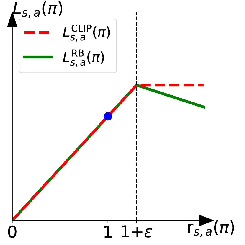
(a) $A_{s,a}>0$

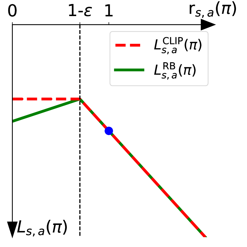
(b) $A_{s,a}<0$

Figure 3: Plots showing $L^{\rm{{\rm{RB}}}}_{s,a}(\pi)$ and $L^{\rm{{\rm CLIP}}}_{s,a}(\pi)$ as functions of the likelihood ratio $\ratio[s,a][\pi]$, for positive advantages (left) and negative advantages (right). The blue circle on each plot shows the starting point for the optimization, i.e., $\ratio[s,a][\pi]=1$. When $\ratio[s,a][\pi]$ crosses the clipping range, the slope of $L^{\rm{{\rm{RB}}}}_{s,a}$ is reversed, while that of $L^{\rm{{\rm CLIP}}}_{s,a}$ is flattened.

Theorem 4

Given parameter $\theta_{0}$, let $\theta_{1}^{{\rm CLIP}}=\theta_{0}+\beta\nabla\hat{L}^{\rm{{\rm CLIP}}}(\theta_{0})$, $\theta_{1}^{{\rm{RB}}}=\theta_{0}+\beta\nabla\hat{L}^{\rm{{\rm{RB}}}}(\theta_{0})$. The set of indexes of the samples which satisfy the clipping condition is denoted as $\Omega=\{t|1\leq t\leq T,|r_{t}(\theta_{0})-1|\geq\epsilon\text{ and }r_{t}(\theta_{0})A_{t}\geq r_{t}(\theta_{{}_{\rm old}})A_{t}\}$. If $t\in\Omega$ and $r_{t}(\theta_{0})$ satisfies $\sum_{t^{\prime}\in\Omega}{\langle\nabla r_{t}({\theta_{0}}),\nabla r_{t^{\prime}}({\theta_{0}})\rangle A_{t}A_{t^{\prime}}}>0$, then there exists some $\bar{\beta}>0$ such that for any $\beta\in(0,\bar{\beta})$, we have

$$\left|r_{t}({\theta_{1}^{{\rm{RB}}}})-1\right|<\left|r_{t}({\theta_{1}^{{\rm CLIP}}})-1\right|.$$ (6o)

Proof  Consider $\phi(\beta)=r_{t}(\theta_{0}+\beta\nabla\hat{L}^{\rm{{\rm{RB}}}}(\theta_{0}))-r_{t}(\theta_{0}+\beta\nabla\hat{L}^{\rm{{\rm CLIP}}}(\theta_{0}))$,

By chain rule, we have

$$\phi^{\prime}(0) =\nabla r_{t}^{\top}(\theta_{0})(\nabla\hat{L}^{\rm{{\rm{RB}}}}(\theta_{0})-\nabla\hat{L}^{\rm{{\rm CLIP}}}(\theta_{0}))$$ (6p)

$$=-\alpha\sum_{t^{\prime}\in\Omega}{\langle\nabla r_{t}({\theta_{0}}),\nabla r_{t^{\prime}}({\theta_{0}})\rangle A_{t^{\prime}}}$$

For the case where $r_{t}(\theta_{0})\geq 1+\epsilon$ and $A_{t}>0$, we have $\phi^{\prime}(0)<0$.

Hence, there exists $\bar{\beta}>0$ such that for any $\beta\in(0,\bar{\beta})$

$$\phi(\beta)<\phi(0)$$

Thus, we have

$$r_{t}(\theta_{1}^{{\rm{RB}}})<r_{t}(\theta_{1}^{{\rm{RB}}})$$

We obtain

$$\left|r_{t}({\theta_{1}^{{\rm{RB}}}})-1\right|<\left|r_{t}({\theta_{1}^{{\rm CLIP}}})-1\right|.$$

Similarly, for the case where $r_{t}(\theta_{0})\leq 1-\epsilon$ and $A_{t}<0$, we also have $\left|r_{t}({\theta_{1}^{{\rm{RB}}}})-1\right|<\left|r_{t}({\theta_{1}^{{\rm CLIP}}})-1\right|$.  

This theorem implies that the rollback function can improve its ability in preventing the out-of-the-range ratios from going farther beyond the range. Ideally, if $\alpha$ is sufficiently large, then the new policy are guaranteed to be confined within the clipping range.

Theorem 5

Let $\pi_{\rm new}=\mathop{argmax}_{\pi}L^{\rm{{\rm{RB}}}}(\pi)$. If $\alpha\rightarrow+\infty$, then for any $(s,a)$ we have

$$\left|r_{s,a}(\pi{{}_{\rm new}})-1\right|\leq\epsilon.$$

Proof  Similar to eq. 6, $L^{\rm{{\rm{RB}}}}_{s,a}(\pi)$ can be rewritten as

$$[left={L^{\rm{{\rm{RB}}}}_{s,a}(\pi)=\empheqlbrace}] {\quad\left({-\alpha\ratio[s,a][\pi]}{+(1+\alpha)(1-\epsilon)}\right)}A_{s,a}$$

$$\quad{\left({-\alpha\ratio[s,a][\pi]}{+(1+\alpha)(1+\epsilon)}\right)}A_{s,a}$$

$$\quad\ratio[s,a][\pi]A_{s,a}$$ otherwise

We prove the converse-positive of this theorem. Assume that given an optimal policy $\pi^{\prime}$, there exists $(s^{\prime},a^{\prime})$ which satisfies $\left|r_{s^{\prime},a^{\prime}}(\pi{{}^{\prime}})-1\right|>\epsilon$. We consider the following cases:

• If $A_{s^{\prime},a^{\prime}}>0$ and $r_{s^{\prime},a^{\prime}}(\pi^{\prime})>1+\epsilon$, then $L^{\rm{{\rm{RB}}}}_{s^{\prime},a^{\prime}}(\pi^{\prime})=-\infty<L^{\rm{{\rm{RB}}}}_{s^{\prime},a^{\prime}}(\pi_{\rm old})=A_{s^{\prime},a^{\prime}}$.

• If $A_{s^{\prime},a^{\prime}}>0$ and $r_{s^{\prime},a^{\prime}}(\pi^{\prime})<1-\epsilon$, then $L^{\rm{{\rm{RB}}}}_{s^{\prime},a^{\prime}}(\pi^{\prime})<(1-\epsilon)A_{s^{\prime},a^{\prime}}<L^{\rm{{\rm{RB}}}}_{s^{\prime},a^{\prime}}(\pi_{\rm old})=A_{s^{\prime},a^{\prime}}$.

Similarly, if $A_{s^{\prime},a^{\prime}}<0$, we also have $L^{\rm{{\rm{RB}}}}_{s^{\prime},a^{\prime}}(\pi^{\prime})<L^{\rm{{\rm{RB}}}}_{s^{\prime},a^{\prime}}(\pi_{\rm old})$.

Finally, we can construct a policy ${\pi^{\prime\prime}}(\cdot|s)=\begin{cases}\pi_{\rm old}(\cdot|s)&\text{if }\exists a\text{ such that }\left|r_{s^{\prime},a}(\pi^{\prime})-1\right|>\epsilon\\ \pi^{\prime}(\cdot|s)&\text{otherwise}\end{cases}$, for which we have $L^{\rm{{\rm{RB}}}}(\pi^{\prime})<L^{\rm{{\rm{RB}}}}(\pi^{\prime\prime})$. This means that $\pi^{\prime}$ is not an optimal solution of $L^{\rm{RB}}$.  

4.2 Trust Region-based PPO (TR-PPO)

As discussed in Question 2, there is a gap between the ratio-based constraint and the trust region-based one: bounding the likelihood ratio is not sufficient to bound the KL divergence. However, bounding the KL divergence is what we primarily concern about, since it is a theoretical indicator on the performance guarantee (see Theorem 1). Therefore, new mechanism incorporating the KL divergence should be taken into account.

The original clipping function of PPO employs the likelihood ratio as the element of the trigger condition for clipping. Inspired by this thinking, we substitute the ratio-based triggering condition with a trust region-based one. Formally, the likelihood ratio is clipped when the policy $\pi$ is out of the trust region,

$${\cal F}^{\rm{\rm{TR}}}({\ratio[s,a][\pi],\delta})=\begin{cases}\ratio[s,a][\pi_{\rm old}]&D_{\rm KL}^{s}(\pi{{}_{\rm old}},\pi)\geq\delta\\ \ratio[s,a][\pi]&\text{otherwise}\end{cases}$$ (6r)

where $\delta$ is the parameter, $\ratio[s,a][\pi_{\rm old}]=1$ is a constant. The incentive for updating policy is removed when the parametrized policy $\pi_{\theta}$ is out of the trust region, i.e., $D_{\rm KL}^{s_{t}}(\theta{{}_{\rm old}},\theta)\geq\delta$. Although the clipped value $\ratio[t][\theta_{\rm old}]$ may make the surrogate objective discontinuous, this discontinuity does not affect the optimization of the parameter $\theta$ at all, since the value of the constant does not affect the gradient.

In general, TR-PPO can combine both the strengths of PPO and TRPO: it is simple to implement (requiring the first-order optimization) while it is somewhat theoretically justified (by the trust region constraint). Like PPO, TR-PPO uses the clipping technique to restrict the policy. The difference is that they use different policy metrics: TR-PPO uses the KL divergence while PPO employs the likelihood ratio. On the other hand, TR-PPO attempts to restrict the policy within the trust region as TRPO does. What makes TR-PPO distinctive is that the trust region-based constraint is used to decide whether to clip the likelihood ratio $\ratio[s,a][\pi]$ or not, without leading to optimizing the objective with a difficult constraint. As a result, it allows using the first-order optimizer like Gradient Descent and significantly reduce the optimization complexity. In other words, it can avoid the complex computation of higher-order optimization which are usually inaccurate (e.g. the second-order optimization of TRPO), resulting in a more stable process of optimization and leading to better solutions.

4.3 Combining TR-PPO with Rollback (Truly PPO)

The trust region-based clipping still possibly suffers from the unbounded KL divergence problem, since we do not enforce any negative incentive when the policy is out of the trust region. Thus we integrate the trust region-based clipping with the rollback operation on KL divergence. We do not use the rollback operation on the likelihood ratio (like PPO-RB) as our goal is to restrict the KL divergence. To make the formalism more intuitive, instead of using the clipping function ${\cal F}$, we use the “case” form to formulate the objective (similar to eq. 6g),

$$[left={{L^{\rm{\rm truly}}_{s,a}(\pi)}=\ratio[s,a][\pi]A_{s,a}-\empheqlbrace}] \alpha D_{\rm KL}^{s}(\pi{{}_{\rm old}},\pi)$$ (6ta)

$$\quad\delta$$ otherwise (6tb)

As the equation implies, the objective generates a negative incentive on the KL divergence when $\pi_{\theta}$ is out of the trust region and the objective is improved. The improvement condition ${\ratio[s,a][\pi]A_{s,a}\geq\ratio[s,a][\pi_{\rm old}]A_{s,a}}$ is the same as the one in eq. 6g (as we have discussed in Section 2.2).

The “rollback” operation on the KL divergence can also be regarded as a penalty (regularization) term, which is also proposed as a variant of PPO (Schulman et al., 2017),

$$L^{\rm{penalty}}_{s,a}(\pi)=\ratio[s,a][\pi]A_{s,a}-\alpha D_{\rm KL}^{s}(\pi_{\rm old},\pi)$$

The penalty-based methods are usually notorious by the difficulty of adjusting the trade-off coefficient. And PPO-penalty addresses this issue by adaptively adjusting the rollback coefficient $\alpha$ to achieve a target value of the KL divergence. However, the penalty-based PPO does not perform well as the clipping-based one, as it is difficult to find an effective coefficient-adjusting strategy across different tasks. Our method introduces the “clipping” strategy to assist in restricting policy, i.e., the penalty is enforced only when the policy is out of the trust region. As for when the policy is inside the trust region, the objective function is not affected by the penalty term. Such a mechanism could relieve the difficulty on adjusting the trade-off coefficient, and it will not alter the theoretical property of monotonic improvement (as we will show below). In practice, we found Truly PPO to be more robust to the coefficient and achieve better performance across different tasks. The clipping technique may be served as an effective method to enforce the restriction, which enjoys low optimization complexity and seems to be more robust.

To analyse the monotonic improvement property, we use the maximum KL divergence instead, i.e.,

$$[left={{L^{\rm{\rm truly}}_{s,a}(\pi)}=\ratio[s,a][\pi]A_{s,a}-\empheqlbrace}] \alpha\max_{s^{\prime}\in{\cal S}}D_{\rm KL}^{s^{\prime}}(\pi{{}_{\rm old}},\pi)$$ (6ua)

$$\quad\delta$$ otherwise (6ub)

in which the maximum KL divergence is also used in TRPO for theoretical analysis. Such objective function also possesses the theoretical property of the guaranteed monotonic improvement. Let $\pi_{\rm new}^{\rm\rm truly}=\mathop{argmax}_{\pi}L^{\rm{\rm truly}}(\pi)$ and $\pi_{\rm new}^{\rm TRPO}=\mathop{argmax}_{\pi}M(\pi)$ denote the optimal solution of Truly PPO and TRPO respectively. We have the following theorem.

Theorem 6

If $\alpha=C\triangleq\mathop{\max}\limits_{s,a}\left|{{A_{s,a}}}\right|{4\gamma}/{{{(1-\gamma)}^{2}}}$ and $\delta\leq\max_{s\in{\cal S}}D_{\rm KL}^{s}(\pi_{\rm old},\pi_{\rm new}^{\rm TRPO})$, then $\eta(\pi_{\rm new}^{\rm\rm truly})\geq\eta(\pi_{\rm old})$.

Proof  First, we prove two properties of $\pi_{\rm new}^{\rm TRPO}$.

• Note that $M(\pi)=E_{s,a}\left[r_{s,a}(\pi)A_{s,a}\right]-\alpha\max_{s^{\prime}\in{\cal S}}D_{\rm KL}^{s^{\prime}}(\pi_{\rm old},\pi).$ As $\pi_{\rm new}^{\rm TRPO}$ is the optimal solution of $M(\pi)$, we have

  $$\footnotesize\mathbb{E}_{a}\left[\ratio[s,a][\pi_{\rm new}^{\rm TRPO}]A_{s,a}\right]\geq\mathbb{E}_{a}\left[\ratio[s,a][\pi_{\rm old}]A_{s,a}\right]\text{ for any }s$$ (6v)

  Suffice it to prove the counter-positive of eq. 6v. Assume $\pi^{\prime}$ is an optimal solution of $M(\pi)$ and there exists some $s^{\prime}$ such that $\mathbb{E}_{a}\left[\ratio[s^{\prime},a][\pi^{\prime}]A_{s^{\prime},a}\right]<\mathbb{E}_{a}\left[\ratio[s^{\prime},a][\pi_{\rm old}]A_{s^{\prime},a}\right]$, then we can construct a new policy

  $$\small{\pi^{\prime\prime}}(\cdot|s)=\begin{cases}\pi_{\rm old}(\cdot|s)&\text{if }\mathbb{E}_{a}\left[\ratio[s,a][\pi^{\prime}]A_{s,a}\right]<\mathbb{E}_{a}\left[\ratio[s,a][\pi_{\rm old}]A_{s,a}\right]\\ \pi^{\prime}(\cdot|s)&\text{otherwise}\end{cases}$$

  We have $M(\pi^{\prime})<M(\pi^{\prime\prime})$, which contradicts that $\pi^{\prime}$ is an optimal policy.

• Besides, by eq. 6v, we can also obtain that for any $s$ there exists at least one $a^{\prime}$ such that ${\ratio[s,a^{\prime}][\pi]A_{s,a^{\prime}}\geq\ratio[s,a^{\prime}][\pi_{\rm old}]A_{s,a^{\prime}}}$. Therefore, by condition (6ua), we have

  $$L^{\rm truly}(\pi_{\rm new}^{\rm TRPO})+\eta(\pi_{\rm old})$$ (6w)

  $$= L^{\rm PG}(\pi_{\rm new}^{\rm TRPO})-\alpha{\max_{s\in{\cal S}}D_{\rm KL}^{s}(\pi{{}_{\rm old}},\pi_{\rm new}^{\rm TRPO})}.$$

Then, we prove that $\pi_{\rm new}^{\rm TRPO}$ is the optimal solution of $Ltruly$. There are three cases.

• For $\pi^{\prime}$ which satisfies ${\max_{s\in{\cal S}}D_{\rm KL}^{s}(\pi{{}_{\rm old}},\pi^{\prime})\geq\delta}$ and there exists some $a^{\prime}$ such that ${\ratio[s,a^{\prime}][\pi^{\prime}]A_{s,a^{\prime}}\geq\ratio[s,a^{\prime}][\pi_{\rm old}]A_{s,a^{\prime}}}$ for any $s$, we have

  $$Ltruly(\pi^{\prime})+\eta(\pi_{\rm old})$$ (6x)

  $$= L^{\rm PG}(\pi^{\prime})-\alpha{\max_{s\in{\cal S}}D_{\rm KL}^{s}(\pi{{}_{\rm old}},\pi^{\prime})}$$ (6y)

  $$\leq L^{\rm PG}(\pi_{\rm new}^{\rm TRPO})-\alpha{\max_{s\in{\cal S}}D_{\rm KL}^{s}(\pi{{}_{\rm old}},\pi_{\rm new}^{\rm TRPO})}$$ (6z)

  $$= Ltruly(\pi_{\rm new}^{\rm TRPO})+\eta(\pi_{\rm old})$$ (6aa)

• For $\pi^{\prime}$ which satisfies ${\max_{s\in{\cal S}}D_{\rm KL}^{s}(\pi{{}_{\rm old}},\pi^{\prime})<\delta}$, we have

  $$Ltruly(\pi^{\prime})+\eta(\pi_{\rm old})$$ (6ab)

  $$= LPG(\pi^{\prime})-\alpha\delta$$ (6ac)

  $$< LPG(\pi^{\prime})-\alpha{\max_{s\in{\cal S}}D_{\rm KL}^{s}(\pi{{}_{\rm old}},\pi^{\prime})}$$ (6ad)

  $$\leq LPG(\pi_{\rm new}^{\rm TRPO})-\alpha{\max_{s\in{\cal S}}D_{\rm KL}^{s}(\pi{{}_{\rm old}},\pi_{\rm new}^{\rm TRPO})}$$ (6ae)

  $$= Ltruly(\pi_{\rm new}^{\rm TRPO})+\eta(\pi_{\rm old})$$ (6af)

• We now prove the case of $\pi^{\prime}$ which satisfies ${\max_{s\in{\cal S}}D_{\rm KL}^{s}(\pi{{}_{\rm old}},\pi^{\prime})\geq\delta}$ and there exists some $s^{\prime}$ such that ${\ratio[s^{\prime},a][\pi^{\prime}]A_{s^{\prime},a}<\ratio[s^{\prime},a][\pi_{\rm old}]A_{s^{\prime},a}}\text{ for any }a.$ We have

  $$\mathbb{E}_{a}\left[L_{s^{\prime},a}^{\rm truly}(\pi^{\prime})\right]$$ (6ag)

  $$= \mathbb{E}_{a}\left[r_{s^{\prime},a}(\pi^{\prime})\right]-\alpha\delta$$ (6ah)

  $$< \mathbb{E}_{a}\left[r_{s^{\prime},a}(\pi_{\rm old})\right]-\alpha\delta$$ (6ai)

  $$\leq \mathbb{E}_{a}\left[r_{s^{\prime},a}(\pi_{\rm new}^{\rm TRPO})\right]-\alpha\max_{s\in{\cal S}}D_{\rm KL}^{s}(\pi_{\rm new}^{\rm TRPO})$$ (6aj)

  $$= \mathbb{E}_{a}\left[L_{s^{\prime},a}^{\rm truly}(\pi_{\rm new}^{\rm TRPO})\right]$$ (6ak)

  We can construct a new policy

  $$\small{\pi^{\prime\prime}}(\cdot|s)=\begin{cases}\pi_{\rm new}^{\rm TRPO}(\cdot|s)&\text{if }s\in\{s^{\prime}\}\\ \pi^{\prime}(\cdot|s)&\text{otherwise}\end{cases}$$

  for which we have

  $$L^{\rm truly}(\pi^{\prime})+\eta(\pi_{\rm old})$$ (6al)

  $$= \mathbb{E}_{s,a}\left[L_{s,a}^{\rm truly}(\pi^{\prime})\right]+\eta(\pi_{\rm old})$$ (6am)

  $$< \mathbb{E}_{s,a}\left[L_{s,a}^{\rm truly}(\pi^{\prime\prime})\right]+\eta(\pi_{\rm old})$$ (6an)

  $$= L^{\rm PG}(\pi^{\prime\prime})-\alpha\max_{s\in{\cal S}}D_{\rm KL}^{s}(\pi^{\prime\prime})$$ (6ao)

  $$\leq M(\pi_{\rm new}^{\rm TRPO})$$ (6ap)

  $$= L^{\rm truly}(\pi_{\rm new}^{\rm TRPO})+\eta(\pi_{\rm old})$$ (6aq)

Finally, by Theorem 1, we have $\eta(\pi_{\rm new}^{\rm\rm truly})=\eta(\pi_{\rm new}^{\rm TRPO})\geq M(\pi_{\rm new}^{\rm TRPO})\geq M(\pi_{\rm old})=\eta(\pi_{\rm old})$.

 

5 Related Work

Many researchers have extensively studied different approaches to enforce the constraint on policy updating. Policy gradient-based methods (Sutton et al., 1999; Kakade, 2001) update the parameter of the policy by several steps, which could be considered as a constraint in the parameter space. Kakade and Langford firstly stated that improving the policy within a region in policy space leads to a better policy. Followed by their work, the well-known trust region policy optimization (TRPO) incorporates a KL divergence constraint on policy, and Wu et al. proposed an enhanced method which uses Kronecker-Factored trust regions (ACKTR). Proximal Policy Optimization (PPO) (Schulman et al., 2017) uses a clipping mechanism to enforce the constraint, which allows using the first-order optimization.

Several studies focus on investigating the clipping mechanism of PPO. In our previous work, we show that the ratio-based clipping with a constant clipping range may fail when the policy is initialized from a bad one. To address this problem, we proposed a method that adaptively adjusts the clipping ranges guided by the trust region criterion. In this paper, we also propose a method based on the trust-region criterion, but we use it as a triggering condition for clipping, which is much simpler to implement. Ilyas et al. performed a fine-grained examination and found that the PPO’s performance depends heavily on optimization tricks but not the core clipping mechanism (Ilyas et al., 2018). However, as we found, although the clipping mechanism could not strictly restrict the policy, it does exert an essential effect in restricting the policy and maintain stability. We provide a detailed discussion with empirical results in Section 6.

Our methods are mostly related to several prior methods of constraining policy. We give detail on the relation and difference between these methods. We make comparisons from the following perspectives: Restriction approach — the form of the objective function designing to restrict the policy, which could decide the optimization complexity; Boundness — whether the method could theoretically bound the policy by the corresponding metric; Policy metric — the metric of the policy difference that the algorithm attempts to restrict. Table 1 summarizes the properties of the algorithms.

Algorithm	Restriction Approach	Optimization	Boundness	Policy Metric
TRPO	constraint	second-order	✓	KL
PPO	clipping	first-order	$\times$	likelihood ratio
PPO-RB	clipping	first-order	✓	likelihood ratio
TR-PPO	clipping	first-order	$\times$	KL
Truly PPO	clipping	first-order	✓	KL
PPO-penalty	penalty	first-order	✓	KL

Table 1: Properties of the algorithms.

5.1 Restriction Approach: constraint vs. clipping vs. penalty

TRPO restricts the policy by explicitly imposing a constraint, whereas the variants of PPO make restrictions by the clipping mechanism. Schulman et al. also proposed a penalty-based method, PPO-penalty, which imposes a penalty on the KL divergence and adaptively adjusts the penalty coefficient (Schulman et al., 2017).

The different restriction approaches could lead to different optimization complexity. To solve the constrained problem, TRPO involves second-order optimization and employs conjugate gradient optimization. Such computation could be inaccurate in high-dimensional tasks, leading to incorrect policy gradient. While the clipping-based and penalty-based methods can use stochastic gradient descent (SGD) to train directly, which are much easier to implement and require relatively less computation.

These different restriction approaches could also result in different solutions. The constraint-based method attempts to find an optimal solution within the policy constraint. And the penalty-based methods can also be interpreted in this way by Lagrangian dual. While the clipping-based methods attempt to find a sub-optimal solution within the policy constraint, as these methods stop updating when the policy violates the constraint. However, in practice, the clipping-based methods usually perform much better than the other two ones. One explanation is that the quality of the solution of the constraint-based methods heavily depends on the optimization, which is usually inaccurate, especially for DNNs. While for the penalty-based methods, it is hard to determine the coefficient of the penalty.

5.2 Boundness

The restriction approach and the optimization method could also affect the boundness on the policy. Both constraint-based and penalty-based methods are guaranteed to bound the policy theoretically. As for the original clipping-based methods, as we have discussed in section 3, it suffers from the unbounded problem. However, by incorporating the rollback operation, such an issue is relieved, and the policy is also guaranteed to be bounded theoretically.

5.3 Policy metric: KL divergence vs. likelihood ratio

These algorithms restrict the policy by a different metric. PPO and its variant with rollback operation (PPO-RB) employ the ratio-based metric, while the other algorithms use the metric of KL divergence. The divergence-based metric, $D_{\rm KL}^{s}(\pi_{\rm old},\pi)=\mathbb{E}_{a}\left[\log\frac{\pi_{\rm old}(a|s)}{\pi(a|s)}\right]\leq\delta$, imposes a summation constraint over the action space; while the ratio-based one, $1-\epsilon\leq\frac{\pi(a|s)}{\pi_{\rm old}(a|s)}\leq 1+\epsilon$, is an element-wise one on each action point. The KL divergence metric is more theoretically justified according to the trust-region theorem. In fact, as we have discussed in Section 3, bounding the likelihood ratio at one action point does not necessarily lead to bounded KL divergence.

In our previous work, we showed that different metrics of the policy difference could result in different algorithmic behavior (Wang et al., 2019b). We found that the ratio-based constraint is prone to make the policy be trapped in a bad local optimum when the policy is initialized from a bad solution. To show this, the constraint $1-\epsilon\leq\pi(a|s)/\pi_{\rm old}(a|s)\leq 1+\epsilon$ can be rewritten as $-\pi_{\rm old}(a|s)\epsilon\leq\pi(a|s)-\pi_{\rm old}(a|s)\leq\pi_{\rm old}(a|s)\epsilon$, which can reflect the allowable change of the likelihood $\pi(a|s)$. We can observe that such constraints impose relatively strict restrictions on actions which are not preferred by the old policy (i.e., $\pi_{\rm old}(a_{t}|s_{t})$ is small). Such bias may continuously weaken the likelihood of choosing the optimal action when the initial likelihood $\pi_{\rm old}(a_{\rm optimal}|s)$ is small. We refer interested readers to Wang et al. (2019b) for further details. While the trust region-based one is averaged over the action space and thus has no such bias. We found it usually could learn better in practice.

6 Experiment

We conducted experiments to investigate whether the proposed methods could improve ability in restricting the policy and accordingly benefit the learning. We will first describe the experimental setup. Then the effect on restricting policy and improving performance will be presented. Finally, comparison with several baseline methods and the state-of-the-art methods will be demonstrated.

6.1 Experimental Setup

To measure the behavior and the performance of the algorithm, we evaluate the likelihood ratio, the KL divergence, and the episode reward during the training process. The likelihood ratio and the KL divergence are measured between the new policy and the old one at each epoch. We refer one epoch as: 1) sample state-actions from a behavior policy $\pi_{\theta_{\rm old}}$; 2) optimize the policy $\pi_{\theta}$ with the surrogate function and obtain a new policy $\pi_{\theta_{\rm new}}$.

We evaluate the following algorithms. (a) PPO: the original PPO algorithm. We used $\epsilon=0.2$, which is recommended by Schulman et al. (2017). We also tested PPO with $\epsilon=0.6$, denoted as PPO-0.6. (b) PPO-RB: PPO with the extra rollback trick. The rollback coefficient is set to be $\alpha=0.3$ for all tasks (except for the Humanoid task we use $\alpha=0.02$). (c) TR-PPO: trust region-based PPO. The trust-region coefficient is set to be $\delta=0.35$ for all tasks (except for the Humanoid task we use $\delta=0.05$). (d) Truly PPO: the coefficients are set to be $\delta=0.03$ and $\alpha=5$ (except for the Humanoid task we use $\delta=0.05$). (e) PPO-penalty: a a variant of PPO which adaptively adjust the coefficient of the KL divergence penalty (Schulman et al., 2017). (f) TRPO: restricting the policy by enforcing a hard constraint. (g) A2C: a classic policy gradient method. (h) SAC: Soft Actor-Critic (Haarnoja et al., 2018), a state-of-the-art off-policy RL algorithm. (i) TD3: Twin Delayed Deep Deterministic policy gradient (Fujimoto et al., 2018), a state-of-the-art off-policy RL algorithm which is competitive with SAC. All our proposed methods and PPO adopts the same implementations given by Dhariwal et al. (2017). This ensures that the differences are due to the algorithm changes instead of the implementations. The implementation details of the proposed methods are given in Appendix A. For SAC and TD3, we adopt the implementations published by the original users (Haarnoja et al., 2018; Fujimoto et al., 2018).

The algorithms are evaluated on continuous control benchmark tasks implemented in OpenAI Gym (Brockman et al., 2016) simulated by MuJoCo (Todorov et al., 2012) and Arcade Learning Environment (Bellemare et al., 2013). For Mujoco, each algorithm was run with 10 random seeds, 1 million timesteps (except for the Humanoid task was 20 million timesteps); the trained policies are evaluated after sampling every 2048 timesteps data. For Atari, the algorithms was run 4 random seeds, 10 million timesteps; we report the episode rewards of the policy during the training process.

6.2 The Effect on Policy Restriction

Question 1

Does PPO suffer from the issue in bounding the likelihood ratio and KL divergence as we have analysed?

In general, PPO could not strictly bound the likelihood ratio within the predefined clipping range. As shown in Figure 4, a reasonable proportion of the likelihood ratios of PPO are out of the clipping range on all tasks. Notably on Hopper, Reacher, and Walker2d, over 30% of the likelihood ratios exceed. Moreover, as can be seen in Figure 5, the maximum likelihood ratios of PPO achieve more than 4 on all tasks (the upper clipping range is 1.2). In addition, the maximum KL divergence also grows as timestep increases (see Figure 6).

Nevertheless, the clipping technique of PPO still exerts an important effect on restricting the policy. To show this, we tested two variants of PPO: one uses $\epsilon=0.6$, denoted as PPO-0.6; another one entirely removes the clipping mechanism, which collapses to the vanilla A2C algorithm. As expected, the maximum likelihood ratios and KL divergences of these two variants are significantly larger than those of PPO. Moreover, the performance of these two methods fail on all the tasks and fluctuate dramatically during the training process (see Figure 10).

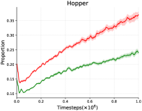
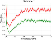
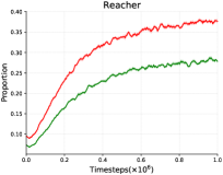
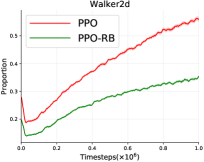
Figure 4: The proportions of the likelihood ratios which are out of the clipping range, i.e., $|r_{t}(\theta_{\rm new})-1|\geq\epsilon$, where $\theta_{\rm new}$ is the parameter at the end of each training epoch. The proportions are calculated over all sampled state-actions at that epoch.

In summary, it could be concluded that although the core clipping mechanism of PPO could not strictly restrict the likelihood ratio within the predefined clipping range, it could somewhat take effect on restricting the policy and benefit the policy learning. This conclusion is partly different from that of Ilyas et al. (2018). They drew a conclusion that “PPO’s performance depends heavily on optimization tricks but not the core clipping mechanism”. They got this conclusion by examining a variant of PPO which implements only the core clipping mechanism and removes additional optimization tricks (e.g., clipped value loss, reward scaling). This variant also fails in restricting policy and learning. However, as can be seen in our results, arbitrarily enlarging the clipping range or removing the core clipping mechanism can also result in failure. These results confirm the critical and indispensable efficacy of the core clipping mechanism.

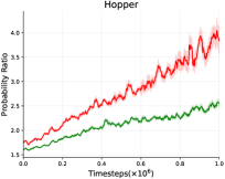
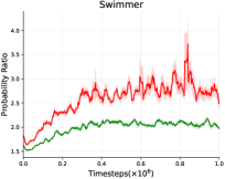
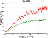
Figure 5: The maximum ratio over all sampled sates of each update during the training process, i.e., $\max_{t}r_{t}(\theta_{\rm new})$.

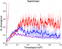
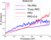
Figure 6: The maximum KL divergence over all sampled states of each update during the training process, i.e., $\max_{t}D_{\rm KL}^{s_{t}}(\theta_{\rm old},\theta_{\rm new})$. The curves of PPO-$0.6$ are clipped as the values can reach 40 which is too large on these tasks.

Question 2

Could the rollback operation and the trust region-based clipping improve its ability in bounding the likelihood ratio or the KL divergence?

In general, our new methods could take a significant effect in restricting the policy compared to PPO. As can be seen in Figure 4, the proportions of out-of-range likelihood ratios of PPO-RB are much less than those of the original PPO during the training process. Besides, the likelihood ratios of PPO-RB are much smaller than those of PPO (see Figure 5). For the trust region-based clipping methods (TR-PPO and Truly PPO), the KL divergences are also smaller than those of PPO (see Figure 6). The maximum KL divergences of Truly PPO are slightly larger than that of TR-PPO on some tasks. This is because Truly PPO retains the term of the likelihood ratio even when the policy is out of the trust region, which could push the KL divergences to increase. However, maintaining the likelihood term could benefit the policy performance of interest, as we will show below.

6.3 The Effect on Policy Performance

LABEL:tab_reward_hit lists learning speed and final rewards on Mujoco tasks. Figure 7 and Figure 8 plots episode rewards during the training process on Mujoco and Atari tasks, respectively.

In general, our Truly PPO method, combining both the rollback operation and the trust region-based clipping, significantly outperform the original PPO on hard tasks characterized by high dimension (e.g., Walker2d with $|{\cal A}|=6$), both in terms of learning speed and final rewards; and Truly PPO is comparable to PPO on the easier tasks with low dimension (e.g., Reacher with $|{\cal A}|=2$). Notably, on Mujoco tasks like Walker2d and Hopper, Truly PPO requires almost 60% and 50% timesteps of PPO to hit the thresholds; and it achieves about 15% and 24% higher final rewards than PPO does on these tasks. On Atari tasks like Breakout, Truly PPO achieves almost twice the final rewards of PPO. We now investigate the effect of the two newly proposed techniques independently.

Question 3

Could the rollback operation benefit policy learning?

We first consider two groups of comparisons: (1) PPO vs. PPO-RB; (2) TR-PPO vs. Truly PPO. The only difference within each group is the existence of the rollback operation.

The results show that the methods with rollback operation outperform the ones without that operation on most of the tasks. For example, Truly PPO achieves fairly better performance than TR-PPO on 5 of 6 Mujoco tasks (see Figure 7) and 5 of 6 Atari tasks (see Figure 8). PPO-RB also performs much better than PPO on 4 of 6 Mujoco tasks. However, the improvements of PPO-RB in comparison of PPO are not significant on Atari tasks. One reason is that the ratio-based constraint may lead to bad local optimum when the policy is initialized from a bad solution (as we have discussed in Section 5.3). While enhancing the ability of restriction may aggravate the issue, especially in the discrete action space tasks.

In summary, the compared methods possess different ability to confine the policy and performs differently in practice. According to the restriction ability in ascending order, the methods can be generally sorted as: without clipping (A2C), with loose clipping (PPO-$0.6$), with proper clipping (PPO, TR-PPO), with rollback operation (PPO-RB, Truly PPO). As we have seen, the performance generally increases as the restriction ability increases. These results confirm the necessity of restricting the policy difference with the old policy. Such improvements may be considered as a justification of the “trust region” theorem — making the policy less greedy to the evaluated value of another policy (old policy) result in a better policy.

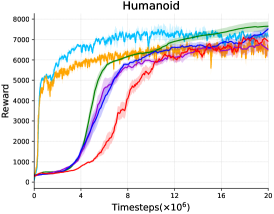
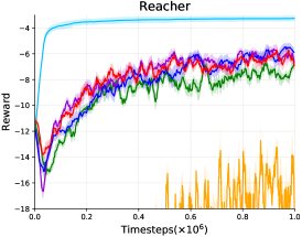
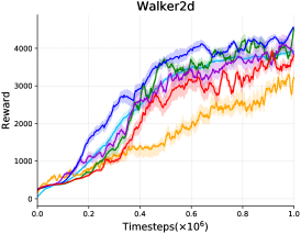
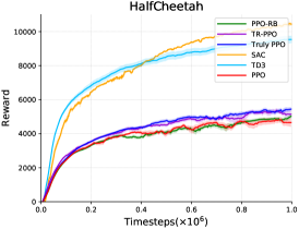
Figure 7: Episode rewards of the policy during the training process averaged over 10 random seeds on Mujoco Tasks, comparing our methods with PPO and the state-of-the-art methods. The shaded area depicts the mean $\pm$ half the deviation.

Question 4

How well do the likelihood ratio-based methods perform compared to the trust region-based ones?

We then consider two groups of comparisons: (1) PPO vs. TR-PPO; (2) PPO-RB vs. Truly PPO. The only difference within each group is whether the method uses constraint by ratio-based metric or KL divergence-based (trust region-based) one.

The results imply that the trust region-based methods perform more sample efficient than the ratio-based ones, and they usually obtain a better policy on most of the tasks. As listed in LABEL:tab_reward_hit (a), TR-PPO learns faster than PPO does on almost all the 6 Mujoco tasks. For example, TR-PPO requires almost half of the episodes than PPO does on Swimmer, and the reductions are more than 30% on Hopper and Walker2d. Similar results can be seen in the comparison of Truly PPO with PPO-RB. Besides, TR-PPO and Truly PPO achieve much higher reward than PPO and PPO-RB do on 4 of the 6 Mujoco tasks (see LABEL:tab_reward_hit (b) and Figure 7) and 5 of 6 Atari tasks (see Figure 8).

As we have discussed in Section 5.3, the constraints with different metrics have different preferences on the actions, leading to the unusual algorithmic behavior. For the ratio-based constraint, the larger likelihood of the action is allowed to update more, making the policy be less random and explore less. While the trust region-based constraint does not has such bias and usually could explore more. To show this, we plot the entropies during the training process in Figure 9. The entropies of trust region-based methods tend to be remarkably larger than those of ratio-based on all tasks. These results confirm the effect on learning behavior with different policy metrics.

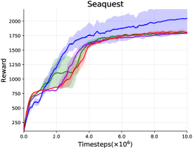
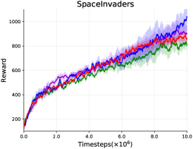
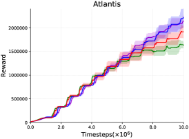
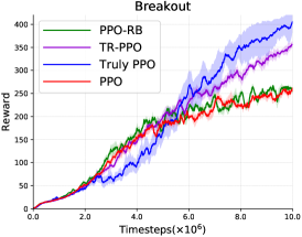
Figure 8: Episode rewards of the policy during the training process on Atari Tasks.

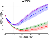
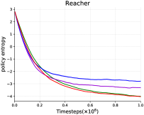
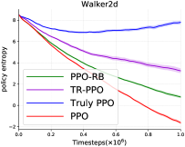
Figure 9: Policy entropy during the training process.

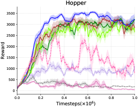
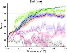
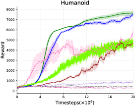
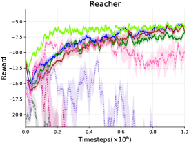
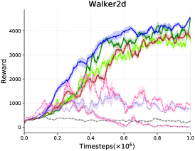
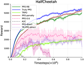
Figure 10: Comparison with several baseline methods. The learning curves show the episode rewards of the policy during the training process on Mujoco Tasks,

6.4 Comparison with Other “Proximal” Approaches

We also compare our variants with TRPO and PPO-penalty which also attempts to enforce proximal constraint. As shown in Figure 10, our methods achieve higher episode rewards than TRPO on 5 tasks. TRPO performs better on low dimensional tasks like Reacher and Swimmer (with $dim({\cal A})=2$ ), whereas it performs much worse on high-dimensional tasks, especially on Humanoid (with $dim({\cal A})=17$). One reason is that the second-order optimization involved in TRPO could be inaccurate, especially on the high-dimensional action space tasks. Such inaccuracy may result in a worse solution. Compared to PPO-penalty, our methods outperform it on all the tasks, which confirms the superiority of the clipping technique that it is more robust across different tasks and requires relatively less effort on hyperparameter tuning.

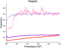
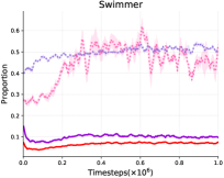
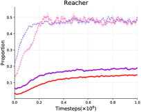
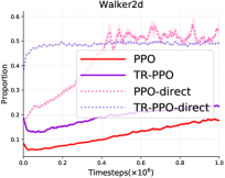
Figure 11: The proportions of the objectives which are not improved but the policy satisfies the clipping condition. Formally, the following conditions are considered: for PPO and PPO-direct, $r_{t}(\theta_{\rm new})A_{t}<r_{t}(\theta_{\rm old})A_{t}$ and $|r_{t}(\theta_{\rm new})-1|\geq\epsilon$; for TR-PPO and TR-PPO-direct, $r_{t}(\theta_{\rm new})A_{t}<r_{t}(\theta_{\rm old})A_{t}$ and $D_{\rm KL}^{s_{t}}(\theta_{\rm old},\theta_{\rm new})\geq\delta$.

6.5 The Minimization Operation

We have discussed the importance of the minimization operation (the improvement condition) of PPO in Section 2.2 (see eq. 4 and eq. 6g). We have stated that without the minimization operation, the likelihood ratios may be trapped in the ones which make the surrogate objective worse. To validate our speculation, we evaluate two variants for PPO, which remove minimization operation for PPO and TR-PPO, named PPO-direct and TR-PPO-direct, respectively. As shown in Figure 10, both these two methods fail on all the tasks (dotted line). We have stated that the minimization operation provide remedy for the case when the objective is not improved while violating the constraint, e.g., $r_{t}(\theta_{\rm new})A_{t}<r_{t}(\theta_{\rm old})A_{t}$ and $|r_{t}(\theta_{\rm new})-1|\geq\epsilon$ ( $D_{\rm KL}^{s_{t}}(\theta_{\rm old},\theta_{\rm new})\geq\delta$ ). We make statistics of these samples. As can be seen in Figure 11, with the minimization operation, the proportions of such un-improved samples are significantly reduced.

6.6 Comparison with the State-of-the-art Methods

We compare our methods with two state-of-the-art methods: Soft Actor Critic (SAC) (Haarnoja et al., 2018) and Twin Delayed Deep Deterministic policy gradient (TD3) (Fujimoto et al., 2018). We use their implementations by the authors, respectively. In general, our methods perform stably across different tasks. As Figure 7 shows and LABEL:tab_reward_hit lists, our methods outperform SAC on 5 tasks except for HalfCheetah. Compared to TD3, our methods perform much better on Swimmer, and are slightly better on Hopper, Walker2d and Humanoid, while performing worse on Reacher and HalfCheetah. On Humanoid task, our methods are not as sample efficient as SAC and TD3 but achieves higher final reward. This may due to that our methods are on-policy algorithms while SAC and TD3 are off-policy ones. Furthermore, our methods require relatively less effort on hyperparameter tuning, as we use the same hyperparameter across most of the tasks. In addition, the variants of PPO are much more computationally efficient than SAC. As can be seen in Table 2, all the variants of PPO require almost 1/10 and 1/50 time of TD3 with 1 million and 20 million timesteps, respectively.

Task	Variants of PPO	SAC	TD3
$1\times 10^{6}$ timesteps	24 min	182 min	238 min
$20\times 10^{6}$ timesteps (Humanoid)	2 h	72 h	108 h

Table 2: Training wall-clock time of the algorithms.

7 Conclusion

Despite the effectiveness of the well-known PPO, it somehow lacks theoretical justification, and its actual optimization behaviour is less studied. To our knowledge, this is the first work to reveal the reason why PPO could neither strictly bound the likelihood ratio nor enforce a well-defined trust region constraint. Based on this observation, we proposed a trust region-based clipping objective function with a rollback operation. The trust region-based clipping is more theoretically justified while the rollback operation could enhance its ability in restricting policy. Both these two techniques significantly improve ability in confining policy and maintaining training stability. Extensive results show the effectiveness of the proposed methods.

In conclusion, our results highlight the necessity to confine the policy difference, leading to a stable improvement of the policy. Besides, different policy metric of the constraint could result in different algorithmic behavior. We found that the KL divergence-based ones outperform the likelihood ratio-based ones. We advocate more studies on how the metric affects the underlying algorithmic behavior. Moreover, the results show that the clipping technique could be served as an effective approach to address the problems with constraint or the one dragged with an adjusted regularization term. We hope our results may inspire approaches for solving these problems. We hope it may inspire approaches for solving other problems with a similar structure. Last but not least, deep RL algorithms have been notorious in its tricky implementations and require much effort to tune the hyperparameters (Islam et al., 2017; Henderson et al., 2018). Our proposed methods are equally simple to implement and tune as PPO but perform much better. They may be considered as useful alternatives to PPO.

Acknowledgments

This work is partially supported by National Science Foundation of China (61976115,61672280, 61732006), AI+ Project of NUAA(56XZA18009), research project no. 6140312020413, Postgraduate Research & Practice Innovation Program of Jiangsu Province (KYCX19_0195).

A Implementation Details

Table 3 and Table 4 list the hyperparameters used for Mujoco and Atari tasks respectively.

Hyperparameter	Value
coefficient of PPO	$\epsilon=0.2$
coefficient of PPO-RB	$\epsilon=0.2$ $\alpha=0.02$ (Humanoid), $0.3$ (Other)
coefficient of TR-PPO	$\delta=0.05$ (Humanoid), $0.035$ (Other)
coefficient of Truly PPO	$\delta=0.05$ (Humanoid), $0.03$ (Other) $\alpha=5$
learning rate	$3\times 10^{-4}$
number of parallel environments	64 (Humanoid) 2 (Other tasks)
timesteps per epoch	1024
initial logstd of policy	-1.34 (HalfCheetah,Humanoid) 0 (Other tasks)
policy	Gaussian
$\lambda$ (GAE)	0.95

Table 3: Hyperparameters for the proposed methods on Mujoco tasks.

Hyperparameter	Value
coefficient of PPO	$\epsilon=\text{LinearAnneal}(0.1,0)$
coefficient of PPO-RB	$\epsilon=\text{LinearAnneal}(0.1,0)$ $\alpha=0.01$
coefficient of TR-PPO	$\delta=\text{LinearAnneal}(0.001,0)$
coefficient of Truly PPO	$\delta=\text{LinearAnneal}(0.0008,0)$ $\alpha=20$
learning rate	$2.5\times 10^{-4}$
number of parallel environments	8
timesteps per epoch	128
policy	CNN
$\lambda$ (GAE)	0.95
coefficient of entropy	0.01

Table 4: Hyperparameters for the proposed methods on Atari tasks.

References

- Bellemare et al. (2013) Marc G Bellemare, Yavar Naddaf, Joel Veness, and Michael Bowling. The arcade learning environment: An evaluation platform for general agents. Journal of Artificial Intelligence Research, 47:253–279, 2013.
- Brockman et al. (2016) Greg Brockman, Vicki Cheung, Ludwig Pettersson, Jonas Schneider, John Schulman, Jie Tang, and Wojciech Zaremba. Openai gym, 2016. cite arxiv:1606.01540.
- Dhariwal et al. (2017) Prafulla Dhariwal, Christopher Hesse, Oleg Klimov, Alex Nichol, Matthias Plappert, Alec Radford, John Schulman, Szymon Sidor, and Yuhuai Wu. Openai baselines. https://github.com/openai/baselines, 2017.
- Fujimoto et al. (2018) Scott Fujimoto, Herke van Hoof, and David Meger. Addressing function approximation error in actor-critic methods. In Jennifer Dy and Andreas Krause, editors, International Conference on Machine Learning (ICML), volume 80 of Machine Learning Research, pages 1587–1596, Stockholmsmässan, Stockholm Sweden, 10–15 Jul 2018. PMLR. URL http://proceedings.mlr.press/v80/fujimoto18a.html.
- Haarnoja et al. (2018) Tuomas Haarnoja, Aurick Zhou, Pieter Abbeel, and Sergey Levine. Soft actor-critic: Off-policy maximum entropy deep reinforcement learning with a stochastic actor. In International Conference on Machine Learning (ICML), pages 1856–1865, 2018.
- Henderson et al. (2018) Peter Henderson, Riashat Islam, Philip Bachman, Joelle Pineau, Doina Precup, and David Meger. Deep reinforcement learning that matters. In National Conference on Artificial Intelligence (AAAI), 2018.
- Hu et al. (2019) Yazhou Hu, Wenxue Wang, Hao Liu, and Lianqing Liu. Reinforcement learning tracking control for robotic manipulator with kernel-based dynamic model. IEEE transactions on neural networks and learning systems, 2019.
- Ilyas et al. (2018) Andrew Ilyas, Logan Engstrom, Shibani Santurkar, Dimitris Tsipras, Firdaus Janoos, Larry Rudolph, and Aleksander Madry. Are deep policy gradient algorithms truly policy gradient algorithms? arXiv preprint arXiv:1811.02553, 2018.
- Islam et al. (2017) Riashat Islam, Peter Henderson, Maziar Gomrokchi, and Doina Precup. Reproducibility of benchmarked deep reinforcement learning tasks for continuous control. arXiv preprint arXiv:1708.04133, 2017.
- Kakade and Langford (2002) Sham Kakade and John Langford. Approximately optimal approximate reinforcement learning. In International Conference on Machine Learning (ICML), volume 2, pages 267–274, 2002.
- Kakade (2001) Sham M Kakade. A natural policy gradient. In Advances in Neural Information Processing Systems (NeurIPS), volume 14, pages 1531–1538, 2001.
- Levine et al. (2016) Sergey Levine, Chelsea Finn, Trevor Darrell, and Pieter Abbeel. End-to-end training of deep visuomotor policies. Journal of Machine Learning Research, 17(1):1334–1373, 2016.
- Liu et al. (2018) Yan-Jun Liu, Shu Li, Shaocheng Tong, and CL Philip Chen. Adaptive reinforcement learning control based on neural approximation for nonlinear discrete-time systems with unknown nonaffine dead-zone input. IEEE transactions on neural networks and learning systems, 30(1):295–305, 2018.
- Mnih et al. (2015) Volodymyr Mnih, Koray Kavukcuoglu, David Silver, Andrei A Rusu, Joel Veness, Marc G Bellemare, Alex Graves, Martin Riedmiller, Andreas K Fidjeland, Georg Ostrovski, et al. Human-level control through deep reinforcement learning. Nature, 518(7540):529, 2015.
- Mnih et al. (2016) Volodymyr Mnih, Adria Puigdomenech Badia, Mehdi Mirza, Alex Graves, Timothy Lillicrap, Tim Harley, David Silver, and Koray Kavukcuoglu. Asynchronous methods for deep reinforcement learning. In International Conference on Machine Learning (ICML), pages 1928–1937, 2016.
- Peters and Schaal (2008) Jan Peters and Stefan Schaal. Reinforcement learning of motor skills with policy gradients. Neural networks, 21(4):682–697, 2008.
- Rai et al. (2019) Akshara Rai, Rika Antonova, Franziska Meier, and Christopher G. Atkeson. Using simulation to improve sample-efficiency of bayesian optimization for bipedal robots. Journal of Machine Learning Research, 20(49):1–24, 2019.
- Schulman et al. (2015) John Schulman, Sergey Levine, Pieter Abbeel, Michael Jordan, and Philipp Moritz. Trust region policy optimization. In International Conference on Machine Learning (ICML), pages 1889–1897, 2015.
- Schulman et al. (2016) John Schulman, Philipp Moritz, Sergey Levine, Michael I. Jordan, and Pieter Abbeel. High-dimensional continuous control using generalized advantage estimation. International Conference on Learning Representations, 2016.
- Schulman et al. (2017) John Schulman, Filip Wolski, Prafulla Dhariwal, Alec Radford, and Oleg Klimov. Proximal policy optimization algorithms. arXiv preprint arXiv:1707.06347, 2017.
- Silver et al. (2017) David Silver, Thomas Hubert, Julian Schrittwieser, Ioannis Antonoglou, Matthew Lai, Arthur Guez, Marc Lanctot, Laurent Sifre, Dharshan Kumaran, Thore Graepel, et al. Mastering chess and shogi by self-play with a general reinforcement learning algorithm. arXiv preprint arXiv:1712.01815, 2017.
- Sutton et al. (1999) Richard S. Sutton, David A. McAllester, Satinder P. Singh, and Yishay Mansour. Policy gradient methods for reinforcement learning with function approximation. In Advances in Neural Information Processing Systems (NeurIPS), pages 1057–1063, 1999.
- Todorov et al. (2012) Emanuel Todorov, Tom Erez, and Yuval Tassa. Mujoco: A physics engine for model-based control. In IEEE/RSJ International Conference on Intelligent Robots and Systems, pages 5026–5033. IEEE, 2012.
- Wang et al. (2019a) Yuhui Wang, Hao He, and Xiaoyang Tan. Truly proximal policy optimization. In Uncertainty in Artificial Intelligence (UAI), 2019a.
- Wang et al. (2019b) Yuhui Wang, Hao He, Xiaoyang Tan, and Yaozhong Gan. Trust region-guided proximal policy optimization. In Advances in Neural Information Processing Systems (NeurIPS), 2019b.
- Williams (1992) Ronald J Williams. Simple statistical gradient-following algorithms for connectionist reinforcement learning. Machine learning, 8(3-4):229–256, 1992.
- Wu et al. (2017) Yuhuai Wu, Elman Mansimov, Roger B Grosse, Shun Liao, and Jimmy Ba. Scalable trust-region method for deep reinforcement learning using kronecker-factored approximation. In Advances in Neural Information Processing Systems (NeurIPS), pages 5279–5288, 2017.