newtx \externaldocument[Q-]quadrics-bowshock
Bow shocks, bow waves, and dust waves. II. Beyond the rip point
Abstract
Dust waves are a result of gas–grain decoupling in a stream of dusty plasma that flows past a luminous star. The radiation field is sufficiently strong to overcome the collisional coupling between grains and gas at a rip-point, where the ratio of radiation pressure to gas pressure exceeds a critical value of roughly 1000. When the rip point occurs outside the hydrodynamic bow shock, a separate dust wave may form, decoupled from the gas shell, which can either be drag-confined or inertia-confined, depending on the stream density and relative velocity. In the drag-confined case, there is a minimum stream velocity of roughly that allows a steady-state stagnant drift solution for the dust wave apex. For lower relative velocities, the dust dynamics close to the axis exhibit a limit cycle behavior (rip and snap back) between two different radii. Strong coupling of charged grains to the plasma’s magnetic field can modify these effects, but for a quasi-parallel field orientation the results are qualitatively similar to the non-magnetic case. For a quasi-perpendicular field, on the other hand, the formation of a decoupled dust wave is strongly suppressed.
keywords:
circumstellar matter – radiation: dynamics – stars: winds, outflows1 Introduction
Stellar bow shocks are predicted to occur whenever a star moves supersonically relative to its surrounding medium, which may either be due to the star’s own motion runaways, e.g., Blaauw, 1961, or due to an independent environmental flow weather vanes, e.g., Povich et al., 2008. Bow shocks are associated with a large variety of different types of stars, for example: AGB stars and red super-giants (Cox et al., 2012); OB stars (Kobulnicky et al., 2017); T Tauri stars (Gull & Sofia, 1979; Henney et al., 2013); photoevaporating protoplanetary disks (García-Arredondo et al., 2001; Smith et al., 2005); neutron stars (Cordes et al., 1993; Brownsberger & Romani, 2014); planetary nebula halos (Ali et al., 2012); and Galactic Center sources (Geballe et al., 2004; Sanchez-Bermudez et al., 2014). The dominant emission mechanism can vary considerably between the different classes of sources, but recombination line radiation such as H, infrared continuum radiation from warm dust, and free-free radio continuum are common (Cantó et al., 2005; Acreman et al., 2016; Meyer et al., 2016). In nearly all cases, stellar bow shocks are easily spatially resolved and mapped, allowing their shapes to be compared with theoretical predictions (Wilkin, 1996; Tarango-Yong & Henney, 2018). A different class of stellar bow shocks are found in interacting binary systems (Stevens et al., 1992), but these typically emit by non-thermal mechanisms and are only resolvable using radio interferometry techniques (Contreras & Rodríguez, 1999; Dzib et al., 2013).
In Henney & Arthur (2019) (hereafter, Paper I) we studied the formation of bows around OB stars by the combined action of their winds and radiation. For the case of strong collisional coupling between gas and dust grains, we showed that three different regimes of interaction are possible, according to the relative values of stellar wind radiative momentum efficiency and the UV optical depth of the bow shell :
-
Wind-supported bow shocks (WBS) where . These are purely hydrodynamic (or MHD) interactions, in which the stellar radiation is dynamically unimportant. This regime dominates for fast-moving stars and for low-density environments.
-
Radiation-supported bow waves (RBW) where . In these optically thin bows, the stellar radiative momentum gradually decelerates the oncoming stream in a broad shell. This regime is important for B stars and weak-wind O stars in moderate density environments ().
-
Radiation-supported bow shocks (RBS) where . These are optically thick shells, internally supported by the trapped stellar radiation pressure. This regime applies to slow-moving O stars in dense environments.
In this paper, we investigate under what circumstances the strong gas–grain coupling might break down, leading to a fourth regime: a separate dust wave outside of the hydrodynamic bow shock (see Fig. 1 of Paper I).
In neutral and molecular regions, the drag forces are relatively weak and so divergent dynamics of gas and grains are frequently found in the context of molecular clouds Hopkins & Lee, 2016; Lee et al., 2017; Mattsson et al., 2019, but see Tricco et al., 2017 and protoplanetary disks (Weidenschilling, 1977; Birnstiel et al., 2010; Dipierro et al., 2018). In ionized regions, the electrostatic forces between charged dust grains and charged gas particles (principally protons) leads to greatly increased drag forces, which tend to maintain a tight coupling between dust and gas (Draine, 2011). However, in a photoionized H ii region around a high-mass star, the dust feels a much larger radiation force than does the gas. This leads to a slow relative drift between the two components in the outer regions of the nebula (Gail & Sedlmayr, 1979; Akimkin et al., 2015, 2017; Ishiki et al., 2018) and a total decoupling very close to the central star (Fig. 8 of Draine, 2011).
With respect to stellar bow shocks, gas–grain decoupling has been previously studied in the context of post-shock flow, where it is the sudden deceleration of the gas that is the primary impetus for the dust to separate. The case of a cool red supergiant was simulated by van Marle et al. (2011), where large grains present in the stellar wind are not stopped in the inner termination shock, but are carried through the contact discontinuity by their inertia, penetrating into the interstellar medium. Katushkina et al. (2017) simulated the opposite case, where grains in the ambient medium become decoupled from the gas after passing the outer bow shock, and subsequently gyrate about the magnetic field, forming filamentary structures (see also Katushkina et al., 2018). In this paper, we study a different decoupling mechanism, where it is the stellar radiation force acting on the grains that causes a separation from the gas before the stream reaches the bow shock. This mechanism was first proposed by Ochsendorf et al. (2014a) to explain the infrared emission arc around the high-mass multiple system Ori.
The plan of the paper is as follows. In § 2 we give some results from Paper I that we will need in later sections. In § 3 we calculate analytical models of the shape of dust waves in the drag-free limit. In § 4 we calculate in detail the grain charging and dynamics, subject to radiation and drag forces, in order to determine the rip point, which is where gas–grain coupling catastrophically breaks down. This is used to determine existence conditions for the presence of a decoupled dust wave. In § 5 we consider the coupling between the grains and the plasma’s magnetic field, and how this effects the existence and structure of dust waves. In § 6 we discuss our results in the context of previous studies. In § 7 we summarise our findings. In Appendix A we provide additional technical information on the numerical calculation of grain trajectories.
2 Recapitulation of Paper I
In Paper I, we found approximate expressions for the bow radius in each of the three regimes discussed in the introduction:
| RBS | (1) | |||||
| RBW | ||||||
| WBS |
In these expressions, we use a fiducial radius
| (2) |
a fiducial optical depth
| (3) |
and a factor that describes the efficiency of the stellar wind as the fraction of the stellar radiation momentum that is converted to wind momentum
| (4) |
Paper I’s equation (11) allows a more exact value for to be found numerically in intermediate cases. Note that is the star–apex distance measured along the symmetry axis of the bow see Tarango-Yong & Henney, 2018 for explanation of nomenclature and discussion of bow shapes, and is calculated in the limit that the momentum transfer occurs at a surface. In cases where the shell’s finite width is significant, , should correspond approximately to the astropause (contact discontinuity) in the WBS regime, or a UV optical depth of unity (as measured from the star) in the RBS regime. The total perpendicular optical depth of the shell to stellar radiation can be found as
| (5) |
In the foregoing, we employ the stellar bolometric luminosity, , wind mass-loss rate, , and terminal velocity, , together with the ambient stream’s mass density, , relative velocity , and effective dust opacity, . It is convenient to define dimensionless versions of these parameters by normalizing to typical values:
where is the mean mass per hydrogen nucleon ( for solar abundances). In terms of these dimensionless parameters, equations (2–4) take the convenient forms:
| (6) | ||||
| (7) | ||||
| (8) |
3 Dust waves in the drag-free limit
(a)
 (b)
(b)
In the optically thin limit, a spherical dust grain of radius situated a distance from a point source of radiation with luminosity spectrum will experience a repulsive, radially directed radiative force (e.g., Spitzer, 1978)
| (9) |
where is the frequency-dependent radiation pressure efficiency111 For absorption efficiency , scattering efficiency , and asymmetry parameter (mean scattering cosine) , we have (e.g., § 4.5 of Bohren & Huffman, 1983). of the grain, and is the speed of light.
If is the only force experienced by the grain, then it will move on a ballistic trajectory, determined by its initial speed at large distance, , and its impact parameter, . For , the grain radially approaches the source with initial radial velocity , which is decelerated to zero at the distance of closest approach, , given by energy conservation:
| (10) |
where we have defined a frequency-averaged single-grain opacity () as
| (11) |
in which is the grain mass and is the bolometric source luminosity. The grain then turns round and recedes from the source along the same radius, reaching a velocity of at large distance. Note that as given by equation (10) is almost the same as Paper I’s equation (6), but with the important difference that it is for a single grain considered in isolation, rather than a well-coupled dusty plasma. Since we are here ignoring collisional effects, there is no pressure, and therefore nothing to stop the spatial coexistence of an inbound and outbound dust stream. For the well-coupled case, this is not possible and a shocked shell must form (see Paper I’s Fig. 5b).
For , the problem is formally identical to that of Rutherford scattering, or (modulo a change of sign) planetary orbits. The method of solution (via introduction of a centrifugal potential term and reduction to a 1-dimensional problem) can be found in any classical mechanics text (e.g., Landau & Lifshitz, 1976, § 14). The trajectory, , is found to be hyperbolic, characterized by an eccentricity, , and polar angle of closest approach, . The trajectory is symmetrical about and can be written as
| (12) |
with a total deflection angle of , which is equal to when .
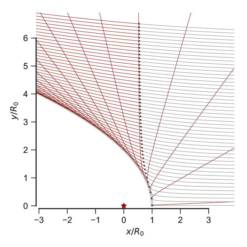
3.1 Parallel dust stream
If the incoming dust grains initially travel along parallel trajectories with varying but the same , then deflection by the radiative force will form a bow-shaped dust wave around the radiation source, as shown in Figure 1. However, the inner edge of the dust wave, is not given by the closest approach along individual trajectories, , but instead must found by minimizing over all for each value of , which yields
| (13) |
This is the polar form of the equation for the confocal parabola, which is discussed in detail in § LABEL:Q-sec:conic and Appendix LABEL:Q-app:parabola of Tarango-Yong & Henney (2018). In that paper, the dimensionless quantities planitude and alatude are introduced as a way of efficiently characterizing bow shapes. The confocal parabola has planitude and alatude of and these are unchanged under projection at any inclination.
3.2 Divergent dust stream
If the dust grains are assumed to originate from a second point source, located at a distance from the radiation source, then the incoming stream will be divergent instead of plane parallel. The individual streamlines are not affected by this change and are still described by equation (12), except that the trajectory axes for are no longer aligned with the global symmetry axis, so we must make the substitution , where (see Fig. LABEL:Q-fig:crw-schema of Tarango-Yong & Henney, 2018). We parameterize the degree of divergence as and, as before, is minimized over all trajectories to find the shape of the bow wave’s inner edge. This time, the result is a confocal hyperbola:
| (14) |
where the eccentricity is (to first order in ) . An example is shown in Figure 1b for . Unsurprisingly, the resulting bow shape is more open than in the parallel stream case, increasingly so with increasing . The planitude and alatude are both equal: ( in Fig. 1b).
3.3 Magnetized dust waves
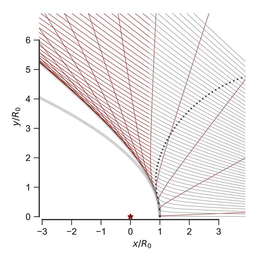
We will show in § 5 that for sufficiently small grains the Larmor magnetic gyration radius, , is small compared with other length scales of interest, and so the grains are effectively tied to the magnetic field lines. In this approximation, we can calculate the grain dynamics in the drag-free limit using as the sole force as above, but this time allowing acceleration only along the field lines. Assuming a uniform magnetic field, the only extra parameter needed is , the angle between the field direction and the direction of the dust stream (assumed to be plane parallel).
We now calculate in detail the grain trajectories in this limit for two cases, with the magnetic field oriented parallel and perpendicular to the stream direction, respectively. In both cases, the stream trajectories are assumed parallel to one another, as in § 3.1. These two cases are sufficient to give a flavor of the effects of a magnetic field on the dust wave structure. Further models at intermediate angles, and which also include the effects of gas drag, are presented in § 5.
3.3.1 Parallel magnetic field
For , the trajectory is identical to the non-magnetic case since the grain velocity and radiation force are both parallel to the field, which yields zero Lorentz force and zero drift. Therefore, the axial turnaround radius, , is still given by equation (10), whatever the value of . For , has a component perpendicular to , which will induce a helical gyromotion around the field lines, but the guiding center must move parallel to the axis if . Thus, the guiding center motion can be found from conservation of potential plus kinetic energy in one dimension:
| (15) |
where is a suitably normalized potential of the projected radiation force along the field lines ( axis, where ):
| (16) |
From equation (15), the trajectory must turn around when , and equation (16) shows that this occurs at the same spherical radius, , for all impact parameters, , so that the inner boundary of the dust wave is hemispherical in shape:
| (17) |
yielding planitude and alatude of . Note, however, that this only applies to streamlines with . For those with , the maximum , which occurs at , is smaller than unity, so that grains on these streamlines do not turn around, although they do slow down temporarily as they go past the star.
The grain density of the inflowing stream follows from mass continuity as:
| (18) |
where for simplicity we assume a single grain species of mass and dust-gas ratio . The outflowing stream has exactly the same velocity profile as the inflowing one, apart from a change of sign for those streamlines that turn round. Therefore, in the region where the two streams co-exist (, , and ), the total density is double that given by equation (18). This is illustrated in Figure 2.
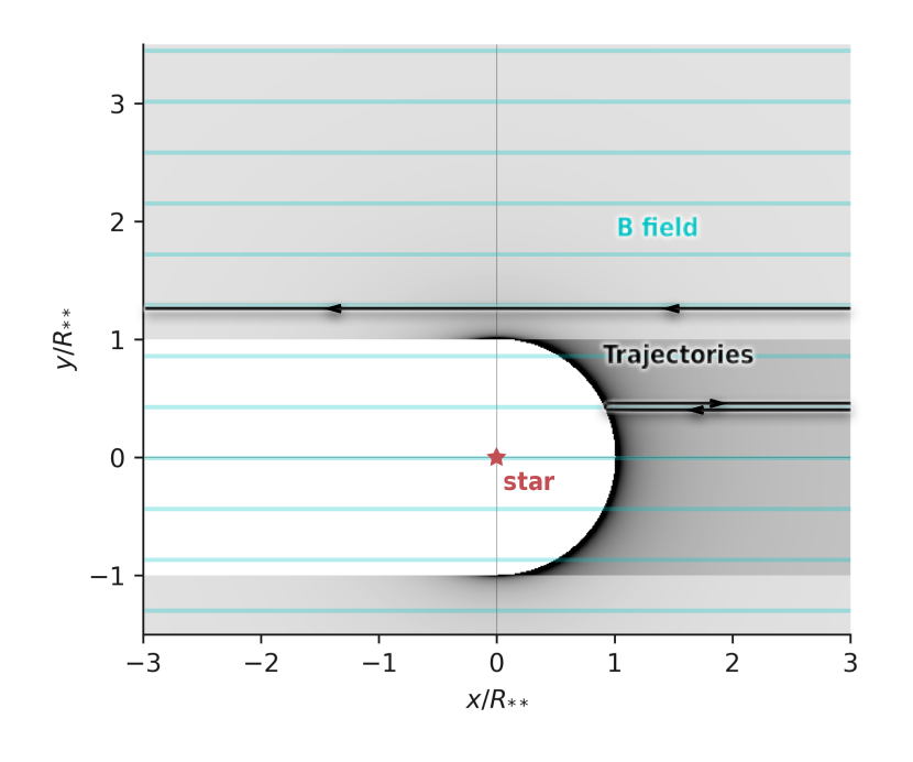
3.3.2 Perpendicular magnetic field
For , the guiding center is forced to move at a constant speed in the direction, so that , while the motion in the direction obeys the ODE:
| (19) |
We have been unable to find an analytic solution to this equation, but a numerical solution is shown in Figure 3a. When the impact parameter is larger than , the trajectories are very similar to in the non-magnetic case (Fig. 1a). As shown in Figure 3b, the interaction of the grain with the radiation field in this large- regime can be approximated as an impulsive acceleration of magnitude and duration , producing a final velocity of . Since the velocity is constant, the total deflection angle is also of order . The overlap of the outgoing trajectories produces a dense concentration of grains at the inner edge, which is roughly parabolic in shape. However, for the remorseless advance of the magnetic field does not allow the grains to slow down and turn round, as they do in the non-magnetic and parallel-field cases. As a result, no dense shell forms in the apex region, but instead there is a diffuse minimum in the density of grains around the star due to the high grain velocities reached there. This means that the apparent morphology of a pure dust wave becomes very sensitive to the radial dependence of the grain emissivity. If this is sufficiently steep, then the apex would coincide with the position of the star, although in practice the presence of a wind-supported bow shock, however small, will complicate the picture. Since there is no unambiguous definition of the star–apex distance in this case, it is not possible to define the shape parameters and either.
4 Gas–grain coupling and decoupling
We now consider how the results of the previous section are changed when drag forces from the gas are taken into account. After considering the general form of these forces in § 4.1, we study the behavior of the grain electrostatic potential in § 4.2 and the nature of the decoupling that occurs for sufficiently strong radiation fields in § 4.3. In § 4.4 we use this information to deduce conditions for the existence of dust waves, and calculate grain trajectories in § 4.5 and estimate the back-reaction on the plasma in § 4.6.
4.1 Drag force on grains
| Regime | Approximate criteria | ||
|---|---|---|---|
| I | Epstein subsonic | and | |
| II | Epstein supersonic | and | |
| III | Coulomb p+ subthermal | and | |
| IV | Coulomb p+ superthermal | and | |
| V | Coulomb e- subthermal | and |
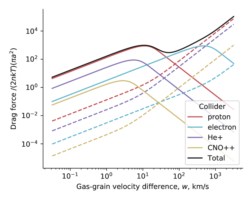
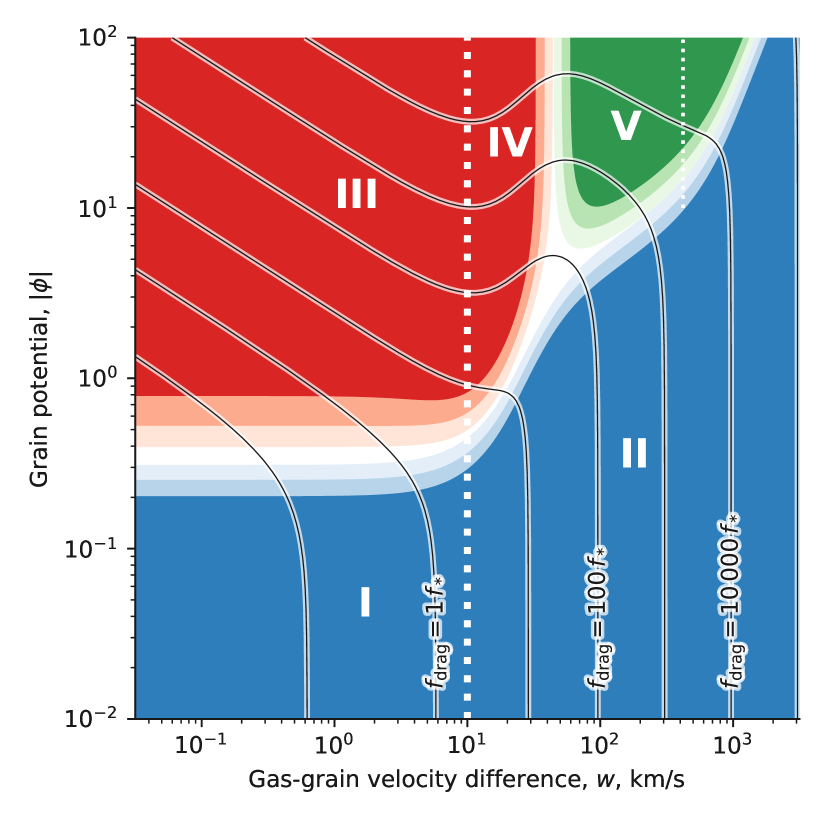
The drag force on a charged dust grain moving at a relative speed through a plasma has contributions from both direct collisions and from electrostatic Coulomb interactions with ions and electrons (Draine & Salpeter, 1979). Full details of the equations and collider species used are given in Appendix A. Results are shown in Figure 4, where dashed lines correspond to direct solid body collisions and solid lines to electrostatic interactions. The latter depend on the grain potential, which is described in dimensionless terms by , the electrostatic potential energy of a unit charge at the surface of a grain of charge and radius , in units of the characteristic thermal energy of a gas particle:
| (20) |
The electrostatic contributions to are proportional to (results are shown for ), whereas the solid-body contributions are independent of . The drag force is put in dimensionless units by dividing by a characteristic force:
| (21) |
which is approximately the ionized gas pressure multiplied by the grain geometric cross section.
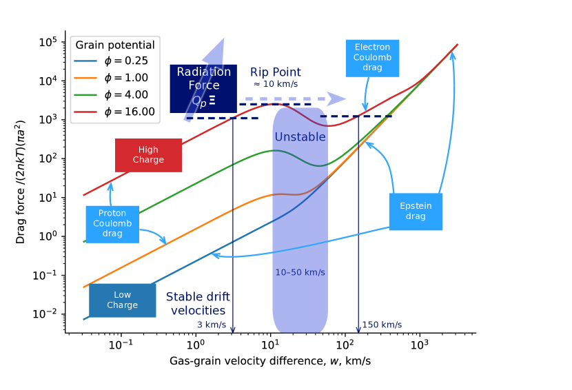
For grains with low electric charge, , the drag force is dominated by direct collisions of protons with the grain (dashed red line in Fig. 4). The gas collisional mean free path is much larger than the grain size, so the drag is in the Epstein regime (Weidenschilling, 1977). As the relative gas–grain slip speed, , increases, first increases linearly with reaching at , then transitions to a quadratic increase in the supersonic regime.
As increases, long-range electrostatic interactions with protons within the Debye radius (Coulomb drag) become increasingly important at subsonic relative velocities, as shown by the solid lines in Figure 4). However, the Coulomb drag has a peak when is equal to the thermal speed of the colliders, which is for protons, giving a maximum strength from equation (48) of
| (22) |
where is the plasma parameter (number of particles within a Debye volume), such that . At highly super-thermal speeds, the Coulomb drag falls asymptotically as . The thermal speed of electrons is higher than that of the protons by a factor of , so that the electron Coulomb drag (solid light blue line) gives a second peak of similar strength, but at . The behavior of in all these different regimes is summarised in Table 1, in terms of and . This is further illustrated in Figure 5, where each of the drag regimes is located on the plane.
| Sp. Type | / | ||||||||
|---|---|---|---|---|---|---|---|---|---|
| B1.5 V | |||||||||
| Main-sequence OB stars | O9 V | ||||||||
| O5 V | |||||||||
| Blue supergiant star | B0.7 Ia |
4.2 Grain charging and gas–grain coupling
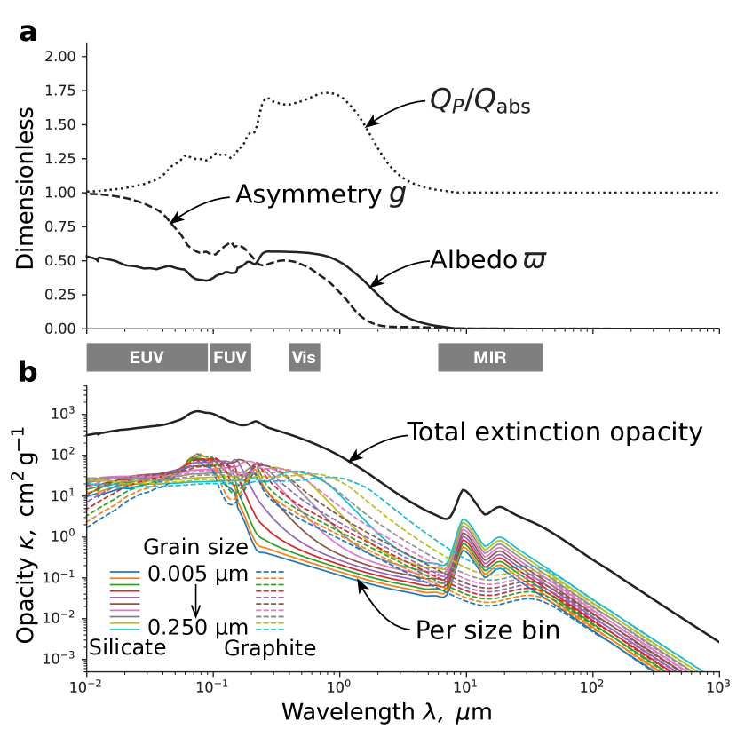
We calculate models of the physical properties of dust grains using the plasma physics code Cloudy (Ferland et al., 2013, 2017), which self-consistently solves the multi-frequency radiative transfer together with thermal, ionization, and excitation balance of all plasma constituents. Cloudy incorporates grain charging as described in Baldwin et al. (1991) and van Hoof et al. (2004) with photoelectric emission theory from Weingartner & Draine (2001a) and Weingartner et al. (2006). We use the default “ISM” dust mixture included in Cloudy, which comprises ten size bins each for spherical silicate and graphite grains in the range to , and which is designed to reproduce the average Galactic extinction curve (Weingartner & Draine, 2001b; Abel et al., 2008). The optical properties of each grain species are calculated using Mie theory (Bohren & Huffman, 1983), assuming solid spheres. The resultant wavelength-dependent extinction properties of the mixture are summarised in Figure 6.
To ascertain the expected variation in grain properties in the circumstellar environs of luminous stars, we calculate a series of spherically symmetric, steady-state, constant density Cloudy simulations, illuminated by the stars listed in Table 2, which are the same ones as used in Paper I. Stellar spectra are taken from the OSTAR2002 and BSTAR2006 grids, calculated with the TLUSTY model atmosphere code (Lanz & Hubeny, 2003, 2007). Simulations are run for hydrogen densities of and assuming standard H ii region gas phase abundances. The calculation is stopped when the ionization front is reached and the inner radius is chosen to be roughly 1% of this.
.
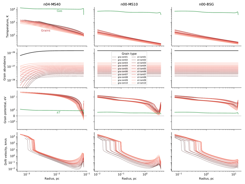
Figure 7 shows resultant radial profiles of dust properties for representative simulations: grain temperature, grain abundance, grain potential, and grain drift velocity. Line types correspond to the different size bins of graphite and silicate grains, as indicated in the key from smallest to largest. The left hand panels show results for a high-density (), compact () region around an early O star, where the grain temperature is very high, especially for the smaller silicate grains, and sublimation significantly reduces the grain abundance in the inner regions (Arthur et al., 2004). The remaining columns show low-density (), extended () regions around main-sequence and supergiant B-type stars, in which the grain temperatures are much lower, ranging from in the outer parts up to in the inner parts.
Unlike the strong differences in thermal properties, the radial dependence of grain electrostatic potential (third row in Fig. 7) is qualitatively similar for all the simulations. The grains are predominantly positively charged, with high potentials ( times the thermal energy of gas particles) close to the star due to the strong EUV and FUV photo-ejection. The potential falls to much lower values in the outer ionized region, as the EUV flux falls off, and then climbs again at the ionization front due to the fall in electron density, while the FUV photo-ejection persists well into the neutral region. There are small differences between the simulations due to the increasing relative importance of the EUV radiation for hotter stars, which leads to a deeper dip in the potential just inside the ionization front for the case, even reaching negative values for some grain species.
Equilibrium drift velocity for each grain species is calculated in the Cloudy simulations using the same Draine & Salpeter (1979) theory as described in § 4.1 and Appendix A. The way that this is implemented by default in Cloudy means that if the only solution at the inner radius is a superthermal one, then the superthermal solution branch is followed as far as possible through the outer spatial zones. We have modified the code so as to instead always prefer the slower subthermal branch whenever multiple solutions are available. This makes more sense than the default behavior for our context, where the grains are moving towards the star and so the radiative force is gradually increasing from an initial low value.
Example results are shown in the bottom row of Figure 7 and again they are qualitatively similar for all the simulations. Close to the star, the radiation force is higher than the upper limit on the Coulomb drag force (eq. [22]), so that the equilibrium drift velocity is exceedingly high. We discuss this situation in greater detail below in § 4.1. Note that such high drift velocities are much higher than any realistic true relative velocity between grains and gas, since they are based on the assumption that the radiation force remains constant while the grain is accelerated, which is not the case under these conditions. Instead, they are simply an indication that the gas and grains have completely decoupled.
As the radial distance from the star increases, the radiation field is increasingly diluted but the grain potential falls only slowly, so eventually a point is reached where an equilibrium between Coulomb drag and radiation force can be established, which corresponds to a discontinuity in the drift velocity. The drift velocity carries on falling towards the outside of the H ii region, but then increases again just inside the ionization front due to the drop in grain potential there.
4.3 Gas–grain separation: drift and rip
In § 3 we calculate the behaviour of an incoming stream of dust grains, subject only to the repulsive radiation force from a star. For an initial inward radial trajectory, the dust grain motion is decelerated and turned around, reaching a minimum radius , given by equation (10). This drag-free radiative turnaround radius, , is smaller for higher initial inward velocities, but is independent of the density of the incoming stream. We are now in a position to see how gas–grain drag will modify this picture.
We introduce the local radiation parameter, , defined as the ratio of direct stellar radiation pressure to gas pressure:
| (23) |
where the last expression corresponds to the optically thin limit. If we define the grain’s frequency-averaged radiation pressure efficiency as
| (24) |
then equations (9) and (21) give the radiation force acting on a grain as
| (25) |
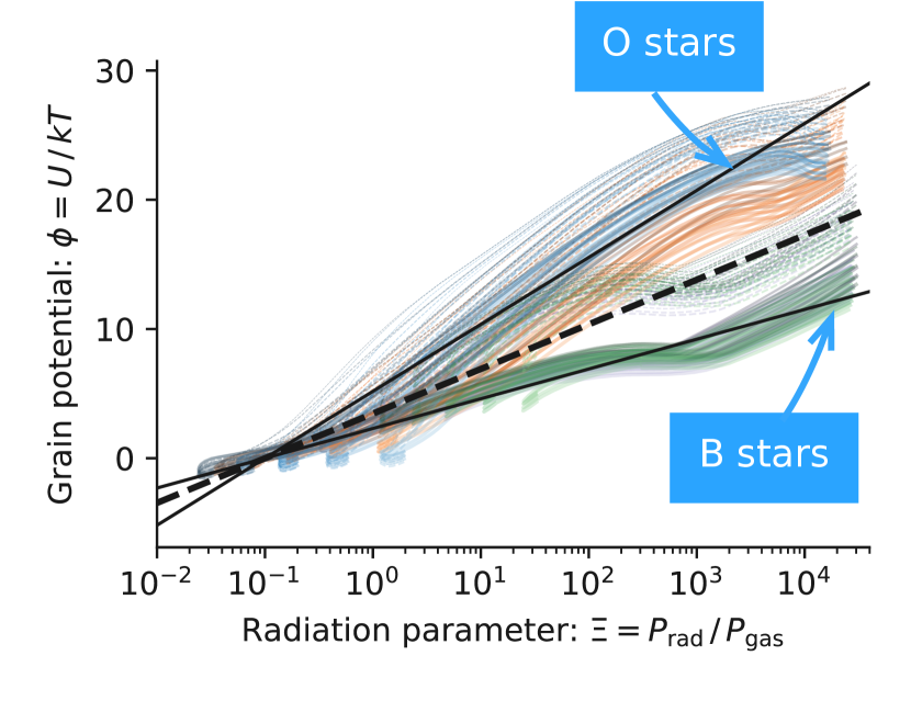
The grain potential , which is crucial for determining (Tab. 1), is due to competition between the photons and the charged particles that interact with the grain. It is therefore reasonable to suppose that should also be primarily determined by . This is confirmed in Figure 8 using the Cloudy simulations of § 4.2, for which we find a slow dependence that can be approximated as
| (26) |
There are also slight secondary dependencies on the grain composition and stellar spectrum. The relationship given in eq. (26) is appropriate for graphite grains and for stellar effective temperatures in the range . For hotter stars than this, should be multiplied by a further factor of , while for silicate grains it should be divided by .
In the outer regions of the photoionized volume around an OB star, close to the ionization front, the radiation parameter is low, with typical value . In this regime, the negative charge current at the grain surface due to electron collisions is roughly in balance with the positive current due to the ultraviolet photoelectric effect (Weingartner & Draine, 2001a), leading to a low grain potential, , which may be positive or negative. The low means that the radiative force is also weak: from equation (25) if at UV wavelengths, which is true for all but the smallest grains. Thus, from the equations for given in Table 1, the radiative force can be balanced by Epstein drag if , leading to a small equilibrium drift velocity, , of the grains with respect to the gas. This drift is much smaller than the inward stream velocities that we are considering (), so the dust follows the gas stream at a slightly reduced velocity (), and (by mass conservation) a slightly increased density. Each grain exerts an exactly opposite force to upon the gas, but since the dust-gas mass ratio, , is small, this produces a negligible acceleration of the gas.
| Grain composition | ||
| Spectrum | Graphite | Silicate |
| B star | ||
| O star | ||
| Calculated from the Cloudy models shown in Figure 10. Uncertainties represent variations with grain size and gas density. | ||
As the dusty stream approaches the star, the radiation parameter will increase, with a dependence of once the stream is well inside the ionization front, assuming roughly constant pressure in the H ii region. This increases (eq. [25]), but also increases the grain potential (eq. [26]) due to the increasing dominance of grain charging by photoelectric ejection. Initially, this results in a lowering of the equilibrium drift velocity to as the Coulomb drag kicks in (see lower panels of Fig. 7). However, at smaller radii the slow logarithmic increase in means that the drift velocity must start increasing again to accommodate the linear increase of . Eventually, exceeds , the maximum drag force that proton Coulomb interactions can provide (eq. [22]). This occurs at a critical value of the radiation parameter, which we denote the rip point: . The process is illustrated in Figure 9, which shows the regions of stability and instability as a function of gas–grain slip velocity as the grain potential and radiation force are increased.
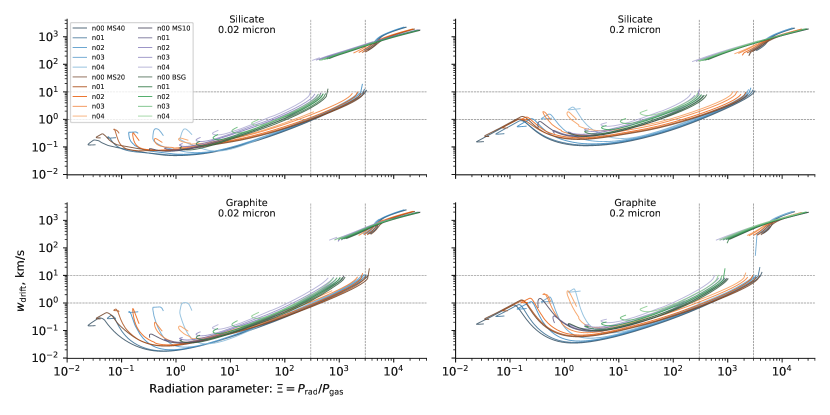
To test these ideas, we plot in Figure 10 the grain drift velocity from the Cloudy simulations as a function of , showing results for four different grain types and for all combinations of stellar parameters and ambient densities for which we have run simulations. It can be seen that the radiation parameter at the rip point is indeed confined to a narrow range. The fundamental explanation for this is that both the charge balance and the force balance are essentially due to competition between the photons and the charged particles that interact with the grain. The small variations in with stellar type and grain composition, which are of order , are listed in Table 3. The gas density and grain size have very little influence on this critical value , with the only exception being the very smallest grains (, not illustrated), which show , but such grains are only minor contributors to the UV opacity for our adopted dust mixture ( in EUV and in FUV, see Fig. 6).
The radius of the rip point, , can be expressed in terms of , the fiducial optically thick bow shock radius (eq. [2]):
| (27) |
where we have made use of equation (23) and the final approximate equality assumes a typical H ii region temperature of .
4.4 Existence conditions for dust waves
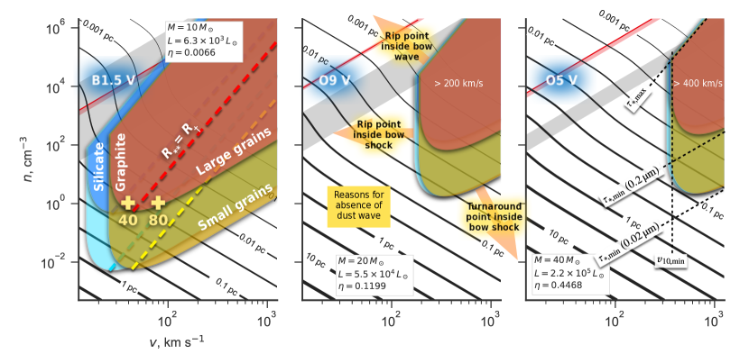
In order for a separate outer dust wave to exist, it is necessary for the grains to decouple from the incoming gas stream before the stream hits the hydrodynamic bow shock caused by the stellar wind. The wind bow shock radius is (eq. [1]), where is the wind momentum efficiency (eq. [8]). Therefore, the condition becomes from equation (27):
| (28) |
For early O main-sequence stars and OB supergiants, the wind efficiency is generally high () and (Tab. 3), so that dust waves can only exist when the stream velocity is very high (). For main-sequence B stars, in contrast, the wind can be much weaker () and is also smaller, so that dust waves are permitted by this criterion for much lower stream velocities: (). The same will be true of the “weak-wind” class of late O main-sequence stars, which also show (see Paper I, § 4).
However, there are other conditions that need to be satisfied in order for the dust wave to exist. For instance, the drag-free turnaround radius must also be outside the bow shock: , otherwise the radiation is incapable of repelling the grain opportunely, even once it has decoupled from the gas. From equation (10), together with Paper I’s equations (2, 3), we find
| (29) |
so the condition becomes
| (30) |
The average value of the factor over the entire grain population must be equal to the dust–gas mass ratio, , but the factor will vary between grains, according to their size and composition.222Recall that is the opacity per unit mass of gas, while is the opacity per unit mass of a particular grain. In both cases, averaged over the stellar spectrum. In particular, it will be relatively larger for the largest grains (), which dominate the total dust mass, and smaller for the smaller grains (), which dominate the UV opacity. Given the dependence of on the stream parameters (eq. [7]), for a given stellar luminosity this condition corresponds to a minimum value for .
A third condition comes from requiring in the radiation bow wave regime (see Paper I’s § 2.1), where . This yields
| (31) |
which, for a given stellar luminosity, corresponds to a maximum value for . Thus, for a given stream velocity that satisfies equation (28), equations (30, 31) determine respectively the minimum and maximum stream density for which a dust wave can exist.
The combined effects of the three conditions are illustrated in Figure 11 for each of the three example main sequence stars from Table 2. Further restrictions on the existence of dust waves arise when the effects of magnetic fields are considered, as will be discussed in § 5 below. Note that the three conditions are restrictions solely on the formation of an outer dust wave, that is, outside of the wind-supported hydrodynamic bow shock. In the case of the equation (30) condition, there is a further possibility: if the gas–grain coupling (and magnetic coupling) is so weak that it is still unimportant at the higher densities found in the bow shock shell, then an inertia-confined inner dust wave may form inside the bow shock, even when . This is similar to the case studied by Katushkina et al. (2017, 2018), which requires simultaneous modeling of the grain dynamics with the magnetohydrodynamics of the bow shock. Note that unlike with equation (30), violation of equation (28) cannot lead to an inner dust wave, since the density compression in the bow shock will reduce the radiation parameter, , which moves the rip point, , to an even smaller radius. Therefore, if radiation has not managed to decouple a grain before it passes through the shock, it is unlikely to be able to do so afterwards.
4.5 Post-rip grain dynamics
We now investigate the trajectory of the dust grain following the catastrophic breakdown of gas–grain coupling at the rip point. Two regimes are possible, depending on the relation between the rip point radius, , and the drag-free radiative turnaround radius, . If , then the grain’s inertia will still carry it in as far as and the initial trajectory will be almost identical to that described in § 3 for the drag-free case. But once the grain has been turned around by the radiation field and pushed out past again, it will recouple to the gas. We will refer to this as an inertia-confined dust wave (IDW). From equations (27, 29, 31), the condition corresponds to
| (32) |
which is indicated by dashed lines in the left panel of Figure 11. If, on the other hand, , then the tail wind provided by the gas carries the grain closer to the star than its inertia would naturally take it. When the grain finally decouples at it experiences a much higher unbalanced , which can initially accelerate it to outward velocities significantly higher than the inflow velocity if . We will refer to this case as a drag-confined dust wave (DDW). As in the IDW case, the expelled grain will eventually recouple to the gas once it moves away from the star.
What happens to the grain after recoupling depends on the sign of when . If this derivative is positive, as is the case in drag regimes II and V (see Tab. 1 and Fig. 5), then the grain can reach a stable equilibrium drift at rest with respect to the star at a point , which we call the stagnant drift radius. If the stream velocity is not excessively high ( when , or when ), then the equilibrium is less than the value at the rip point, requiring a lower value of the radiation parameter: . The resultant stagnant drift radius is therefore outside the rip point: . Of course, a static equilibrium is only possible when the impact parameter is exactly zero. Otherwise, there will be an unbalanced lateral component of the radiation force, which will cause a sideways drift. However, as we show below, strong coupling to the magnetic field means that the strictly on-axis calculation is a reasonable approximation over a range of impact parameters in the case where the angle between the magnetic field direction and the stream velocity is not too large.
On the other hand, if when , then the equilibrium is unstable and no stagnant drift is possible. This occurs for drag regime IV, which applies when and , as illustrated in Figure 9. There is also a second unstable regime (partially visible in the upper-right corner of Fig. 5), which is related to the thermal peak in the electron Coulomb drag when and . This is not relevant to bow shocks around OB stars since does not reach such high values, but it may apply in other contexts, such as outflows from AGN, where grain potentials as high as can be achieved (Weingartner et al., 2006).
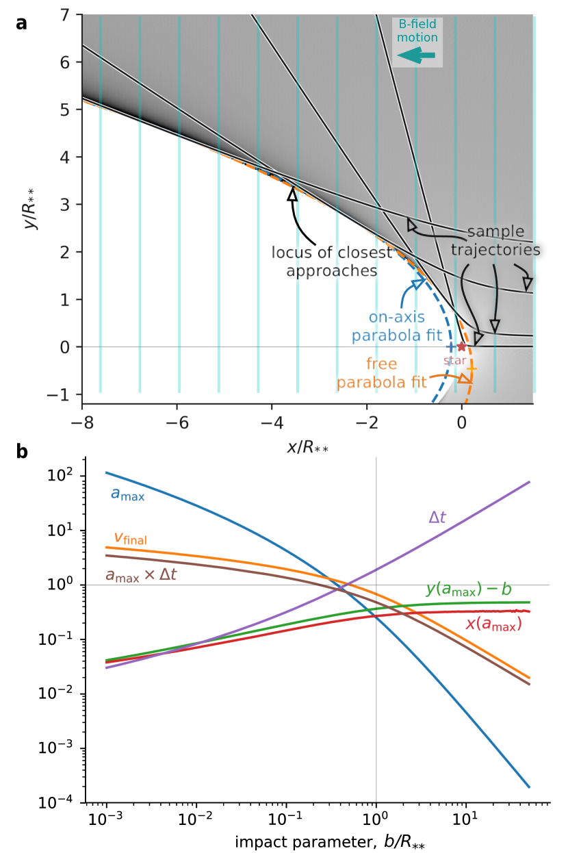
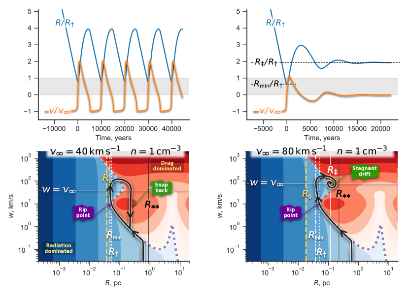
An example of each of these two behaviors is illustrated in Figure 12. The left panels show the case where , which is in the unstable regime, resulting in periodic “limit-cycle” behavior (the parameters of this model correspond to the yellow “plus” symbol labeled “40” in the left panel of Fig. 11). During the grain’s first approach, it starts to follow a phase trajectory (lower left panel) along the contour, corresponding to equilibrium drift, in which the grain begins to move a few slower than the gas stream. Then, when it reaches the rip point (, ) it suddenly experiences a large unbalanced outward radiation force (blue region of phase space in Fig. 12). The grain’s inward momentum carries it to the point , before it is expelled at roughly twice the inflow speed. However, after moving outward, it finds itself in a drag-dominated region of phase space (red in the figure), and so recouples to the inflowing gas stream. The recoupling initiates gradually, as the grain’s outward motion is slowed and turns around, but is completed suddenly once again falls below , in what we term snap back. The net result is that the grain has returned to exactly the same phase track that it started in on, and so repeats the cycle indefinitely.
The right panels of Figure 12 show the case where the stream velocity is doubled to , but all other parameters remain the same. At this velocity, the equilibrium drift is stable and so the grain can achieve a stagnant drift solution, where it is stationary with respect to the star. The trajectory during the first approach is similar to the previous case, except that the overshoot of the rip point is greater, so that in this case. This is a consequence of the fact that the rip point is closer to the drag-free turnaround radius ( is larger than in the lower velocity case), so that the grain inertia is relatively more important. A second consequence of this is that the speed of the initial expulsion is not so large, being only a little higher than the inflow velocity. The qualitative difference between the two cases emerges after the first recoupling: instead of the snap back and endless limit cycle, the grain oscillates about the stagnant drift radius with ever decreasing amplitude, so that after a few oscillation periods it has come to almost a complete rest.
4.6 Back reaction on the gas flow
So far we have ignored the effect of the drag force on the gas stream itself, but it is clear that this must become important as approaches , since that is the point where the dust wave transitions to a bow wave, in which the dust and gas are perfectly coupled. A full treatment of this problem would require solving the hydrodynamic equations simultaneously with the equations of motion of the dust grains, which is beyond the scope of this paper. Instead, we outline a heuristic approach that qualitatively captures the physics involved.
The maximum drag force experienced by a grain is at the rip point. Since the grain follows a zero-net-force phase track up until that point, this can be written with the help of equations (9, 10) as
| (33) |
The timescale of the flow can be characterized by the crossing time , but the residence time of the grain at the bow apex will be several times larger than this (see previous section). On the other hand, the average drag force during this residence will be several times smaller than if , which is typically the case. We therefore parameterize our ignorance via a dimensionless factor, , which we expect to be of order unity, and write the total impulse imparted to the grain by drag as
| (34) |
By Newton’s Third Law, an equal and opposite impulse is imparted to the gas, which will act to decelerate the gas stream as it decouples from the grains. Realistically, should be summed over the grain size distribution, but for simplicity we assume that all grains are identical, so that the mass of gas that accompanies each grain is given by
| (35) |
If the gas remains supersonic after decoupling, then thermal pressure can be ignored and the gas will suffer a change in momentum equal to , so that its velocity is reduced by , which by equations (27, 29, 31, 34, 35) is
| (36) |
This deceleration reduces the gas stream’s ram pressure before it interacts with the central star’s stellar wind. The radius of the dust-free bow shock formed by this interaction is therefore increased by a factor with respect to the value given by equation (1), yielding
| (37) |
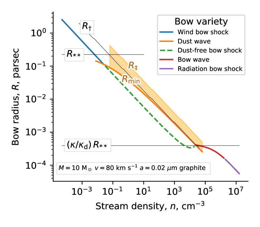
An example is illustrated in Figure 13, where the dust-free bow shock radius is shown by the green dashed line as a function of stream density, . This is calculated for fixed stream velocity and grain and star properties, so that (eq. [7]). In order for to match the dust-wave and bow-wave radii at the point where they cross at , we find is required. It can be seen that the gas deceleration is negligible over most of the density range for which a separate dust wave arises. Only for does begin to curve up from the general trend, becoming essentially flat at a value until full-coupling is established at . Note, however, that the treatment described here is very approximate: it does not take into account the shock that must form once reaches an appreciable fraction of and, additionally, it includes a factor, , whose value has not been rigorously justified. More detailed modeling is required to fully understand the bow behavior in this transition regime.
5 Magnetic coupling of grains
It remains to calculate in detail the effects on grain dynamics of the plasma’s magnetic field, in order to justify the approach taken in § 3.3 and extend those results to include the effects of drag forces from the gas. The Lorentz force on charged grains due to a magnetic field is
| (38) |
The direction of the force is perpendicular both to the magnetic field, , and to the relative velocity, , of the grain with respect to the plasma. If and (as seen by the grain) are changing slowly, compared with the gyrofrequency, , then the grain motion perpendicular to is constrained to be a circle of radius equal to the Larmor radius:
| (39) |
where and is the perpendicular component of . The component of parallel to is unaffected by , so the resultant trajectory is helical.
The relative importance of the magnetic field can be characterized by the ratio of the Larmor radius to the minimum radius, , reached by the grain in the dust wave (see § 4.5), where for drag-confined dust waves (DDW), or for inertia-confined dust waves (IDW). We write the field strength in terms of the Alfvén speed,
| (40) |
and the grain charge in terms of the potential (eq. [20]) to obtain
| (41) |
and
| (42) |
where , is the grain material density in , and we have made use of equations (6, 10, 27).
If , then the grains are so strongly coupled to the field that they can be treated in the guiding-center approximation, in which the trajectory is decomposed into a tight circular gyromotion around the field lines, plus a sliding of the guiding center along the field lines, which is governed by the radiation and drag forces. The radiation force will also produce an out-of-plane drift, given by
| (43) |
but from equations (39, 9, 10) it follows that
| (44) |
so it is valid to ignore this drift in the limit of small . This is the limit that was applied in § 3.3 for the case of zero drag. In the opposite limit, , magnetic coupling is so weak that the non-magnetic results of § 4 are scarcely modified. Assuming and adopting a threshold of , equations (41, 42) can be transformed into conditions on the stream velocity (in ) where tight magnetic coupling will apply: , where
| (45) | ||||
in which we have substituted typical values of the minor parameters , , , , .333The most significant systematic variation in from these suppressed parameters is due to grain composition, yielding slightly higher values for graphite than for silicate (). It is apparent that is very sensitive to the grain size. For instance, taking a typical H ii region value of (Arthur et al., 2011) and (Tab. 2, B1.5 V star), then for the drag-confined case for grains but for grains. Thus, for typical stream velocities of , the small grains are always tightly coupled to the magnetic field, but the large grains are only loosely coupled for the faster streams.
5.1 Grain trajectories with tight magnetic coupling
We can now investigate how the results of the section 4 are modified by magnetic fields in the tight coupling limit. For simplicity, we assume a uniform field in the incoming stream, with field lines oriented at an angle to the velocity vector that defines the bow axis. We also assume a super-alfvénic stream, , so that the radius, , of the wind bow shock is unaffected by the magnetic field, and additionally assume , so that the back-reaction of the grain drag on the plasma is negligible (§ 4.6) and remains uniform in magnitude and direction in the dust wave region, outside of the bow shock.
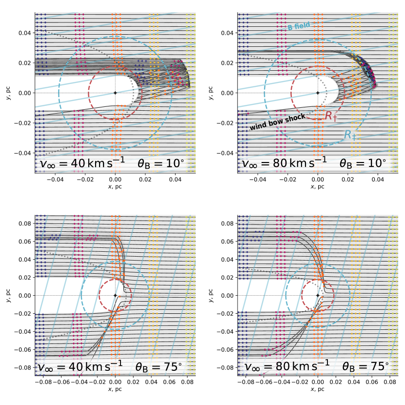
In § 3.3, we derived analytic and semi-analytic results in the limit of zero gas–grain drag, which is appropriate for inertia-confined dust waves. The resultant dust wave structure is highly dependent on the field orientation. For a parallel field (Fig. 2), the apex of the dust wave occurs at the same point, , as in the non-magnetic case, but the shape of the dust wave wings is more closed, being hemispherical rather than parabolic in shape. For a perpendicular field (Fig. 3), on the other hand, grains in the apex region are dragged very close to the star and no dust wave forms there. A dust wave can form in the wings, with impact parameter , which is roughly parabolic in shape, but more swept-back than in the non-magnetic case. Whether such a dust wave will exist in practice depends critically on the size and shape of the interior MHD wind-supported bow shock.
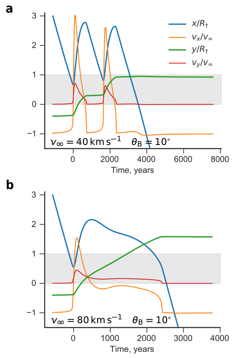
In Figures 14 and 15 we show example results for drag-confined dust waves, which are calculated by numerically integrating the grain’s equation of motion, as described in Appendix A. Apart from the inclusion of the magnetic field, the model parameters are the same as used in Figure 12, with the exception that the stream density is increased to .444The reason for using a higher density is to decrease the amplitude of the radial oscillations of the trajectories, which allows the dust wave structure to be more clearly perceived in the figures. This time, we use quasi-parallel () and quasi-perpendicular () field orientations. The quasi-parallel field is most similar to the non-magnetic case, and the models shown in the two upper panels of Figure 14 closely mirror the cases shown in Figure 12, with a limit cycle behavior when and stagnant drift when .
The principle difference from the 1-D axial trajectories discussed in § 4.5 is that the small misalignment of from the incident stream direction causes a slow sideways migration, which puts a finite limit on the time a grain can reside in front of the star. This can be appreciated more clearly in Figure 15, which shows the grain position and velocity along a sample streamline with initial impact parameter for the two quasi-parallel models. In panel a, corresponding to , we see the same rip-and-snap-back cycle of de-coupling and re-coupling that was discussed previously, but only two periods of the cycle are completed before the grain’s lateral migration takes it as far as , at which point nothing can stop the gas stream from dragging it past the star and away. All told, the grain remains in the apex region for about times longer than the crossing time, .
In panel b, corresponding to , the grain settles for a while around the stagnant drift radius, , after the initial rip and turn around. Again, it slowly migrates sideways, and eventually recouples to the incident stream, but this time after reaching . The grain residence time in the apex region, measured in crossing times, is slightly longer than in panel a, but is of the same order. In both these cases a second, exterior dust shell is formed in addition to the hemispherical one produced by the initial turn around inside . In the limit-cycle case, it forms at the snap-back point, while in the stagnant-drift case, it forms at and is significantly denser than the interior shell (upper right panel of Fig. 14).
The assumptions behind these models break down when the grain trajectory intersects the outer shock of the dust-free wind-supported bow shock. The increased gas pressure in the bow shock shell will reduce , which is likely to cause gas–grain recoupling in the case of drag-confined dust waves (see also discussion in the final paragraph of § 4.4). However, detailed modeling of this requires magnetohydrodynamical simulations, which are beyond the scope of this paper. In Figure 14 we show in gray dotted lines the Wilkinoid surface (Wilkin, 1996), which is an approximation to the shape of the inner bow shock, see Tarango-Yong & Henney (2018). It can be seen that the majority of dust streamlines do not cross this surface until well into the wings of the bow, so that a separate exterior dust wave can exist for this quasi-parallel magnetic field orientation.
This is no longer the case for the quasi-perpendicular field orientation, as illustrated in the lower panels of Figure 14, where the behavior is similar to the perpendicular inertia-confined case studied in § 3.3.2. Although the grains decouple from the gas inside the rip point, for small impact parameters the magnetic geometry does not allow the radiation field to expel them until they are much nearer to the star. Since the inner wind-supported bow shock radius is only a few times smaller than , it is possible that they will pass through the shock surface and re-couple before expulsion can occur. For the model (lower left panel), all of the streamlines with impact parameters intersect the Wilkinoid surface before they are deflected, and so no separate dust wave would form in this case. For the model (lower left panel), some of the streamlines (mainly those with ) do manage to avoid crossing the bow shock surface, so it is possible that a dust wave may still form, although it would be on only one side of the axis.
6 Discussion
In this section we briefly discuss our predictions for the appearance of dust waves and place our results in the context of previous work on gas–grain coupling in the environs of high-mass stars. We concentrate on conceptual and theoretical aspects, postponing empirical questions about particular sources for later papers.
6.1 Predicted appearance of dust waves
By definition, dust waves do not correspond to any structure in the gas and so are only detectable via the mid-infrared thermal emission of the grains. The emissivity is proportional to the grain density but also depends on the grain temperature, which is a decreasing function of radius, , from the star see, for example, synthetic observations in Mackey et al., 2016; Acreman et al., 2016; Meyer et al., 2017. In radiative equilibrium, the bolometric emissivity is proportional to the stellar flux , but the radial dependence of the monochromatic emissivity will be much steeper than this on the short-wavelength side of the average grain thermal spectrum. With this in mind, we can crudely estimate the appearance of the example dust waves calculated in §§ 3 and 5.1.
In the inertia-confined case, the radius is proportional to the single-grain opacity and will therefore vary with grain size and composition. For a spherical grain of size and solid density , equation (11) yields
| (46) |
The radiation pressure efficiency is for , but falls as for smaller grains (e.g., Fig. 7 of Draine, 2011). Therefore, all the smallest grains will form the dust wave at the same point, but grains larger than will be spread out with . It might be thought that this would produce a very broad diffuse appearance to the dust wave, but this is mitigated by the fact that it is the smaller grains that dominate the UV opacity and mid-IR emissivity. Also, the larger grains may be destroyed by radiative torques (see § 6.4). For the drag-confined case, the situation is clearer since the dust wave will form just inside the rip point, , which is relatively insensitive to the grain size.
The effect of a roughly parallel magnetic field is mainly seen in the shape of the dust wave, which becomes hemispherical (Fig. 2) instead of parabolic as was found in the non-magnetic case (Fig. 1). Interestingly, this effect is the opposite of what is seen in simulations of MHD bow shocks (Meyer et al., 2016), where a parallel B-field leads to flatter-nosed bow shapes with a high planitude see Fig. 25 of Tarango-Yong & Henney, 2018. Figure 14ab shows that the field orientation has a similar effect on the dust wave shape for drag-confined magnetic dust waves, but with the added complication that a second dense shell forms on one side of the axis at the stagnant drift radius, , in cases where . However, since is several times larger than , the emission from this outer shell is likely to be weak, given the steep radial dependence of the mid-IR emissivity discussed above.
6.2 Gas–grain dynamics in H ii regions
The distinction that we draw in § 4.4 between inertia-confined dust waves and drag-confined dust waves is novel. However, the concept of the rip point can be found in previous works, although not under that name and it has generally been assumed to be of little interest. For instance, Figure 8 of Draine (2011) clearly shows the discontinuity in drift velocity that occurs at small radii within an H ii region (differences from our own Figs. 7 and 10 are due to Draine’s assumption of constant grain potential). However, the region of supersonic drift involves a very small fraction of the total dust in the H ii region, so it was not relevant to the concerns of that paper. Similarly, in § 3.1 of Hopkins & Squire (2018b) the possibility is raised of a “decoupling instability” in the case that coupling strength decreases with increasing slip velocity, but they go on to dismiss this as physically irrelevant. On the contrary, we show in this paper that it is relevant so long as the grain potential is high, so that a distinct local maximum occurs in the drag-versus-velocity profile (see Fig. 9). In § 9 of Hopkins & Squire (2018a), various issues relating to grain charging and drag are discussed. The quantity from § 9.1.4 of that paper is the same as our radiation parameter, . In § 9.2.3 they give an expression for the critical radius that divides subsonic from supersonic drift, which is exactly equivalent to our equation (27) for the rip point radius. The parameters assumed by Hopkins & Squire yield , which is within the range of values that we find for O stars in Table 3.
Akimkin et al. (2017) studied the effect of radiation pressure on the time-dependent evolution of an H ii region, taking full account of dynamical coupling between grains and gas, thus extending a previous study (Akimkin et al., 2015) that had ignored the back-reaction on the gas (see our § 4.6). They found that the dust completely decouples from the gas in the zone around the star ( on timescales ), which produces an inner dust hole but partially eliminates the inner gas density hole that is found in models that assume perfect coupling (Mathews, 1967; Draine, 2011; Kim et al., 2016). The decoupling is more pronounced for stars of lower effective temperature, which is probably related to the fact that we find the critical radiation parameter to be lower for B stars than for O stars (Table 3). A similar dust hole for the central region is found by Ishiki et al. (2018).
The gas–grain decoupling that we have discussed so far occurs at high radiation parameter, , but there is another regime of potential decoupling that occurs at low . It has long been recognized (Gail & Sedlmayr, 1979) that Coulomb gas–grain coupling should weaken in the outer zones of an H ii region due to the fact that the grain potential passes through (or close to) zero as a result of electron collisions becoming competitive with photoelectric ejection as the radiation field weakens. This is the regime around in Figure 10, giving drift velocities of order for larger grains (), which may be sufficient to produce significant spatial variations in grain abundance on Myr timescales (Ishiki et al., 2018). It remains to be seen whether this is still true once effects that have been neglected in existing models are accounted for, such as the H ii region’s magnetic field (Krumholz et al., 2007; Arthur et al., 2011; Gendelev & Krumholz, 2012) and internal turbulence (Arthur et al., 2016). On the other hand, grain abundance variations may be enhanced by the resonant drag instability (Squire & Hopkins, 2018; Hopkins & Squire, 2018a). Yet another regime of potential decoupling occurs in the neutral shell outside the H ii region (Gustafsson, 2018), but since the drift velocity in both these cases is much less than interesting values of the stream velocity, , neither low- regime is relevant to dust waves.
6.3 Gas–grain dynamics in stellar bows
The term dust wave was first coined to described the radiative decoupling of grains from the plasma flowing past a massive star by Ochsendorf et al. (2014a), who attempted to explain the infrared emission arc around Ori. The concept was subsequently applied to additional dust arcs in RCW 82 and RCW 120 (Ochsendorf et al., 2014b) and a refined model was applied to further observations of Ori (Ochsendorf & Tielens, 2015). These works provided the inspiration for the present paper, where we have attempted to take a more a priori and systematic approach to the problem, including factors such as the Lorentz force that were neglected by Ochsendorf et al..
The most detailed simulations to date of the combined dynamics of dust, gas, and magnetic field in an OB bow was carried out by Katushkina et al. (2017), who followed the trajectories of dust particles after passing through an MHD bow shock, under the influence of the stellar radiation force and Lorentz force. The gas is decelerated in the shock, but the dust initially carries on with its pre-shock motion, which produces a relative velocity with respect to the plasma. The component of this velocity perpendicular to the magnetic field induces gyration about the field lines (cf § 5), which forms filaments of enhanced dust density that are oriented perpendicular to the bow axis and with characteristic separation equal to the bulk plasma velocity times the gyration period. In Katushkina et al. (2018), similar such simulations are applied to observations of the runaway B1 supergiant Cas, moving at , in order to explain the filaments of infrared dust emission seen at . It is found that the simulations can only fit the observations with very large dust grains () and a very strong perpendicular magnetic field . The stellar parameters of Cas are roughly those given in the last row of Table 2 and the observed radius of the dust arc (assumed to correspond to the astropause) is for a distance of . The Katushkina et al. simulations do not explicitly include the Coulomb drag force on the dust grains, although our own results (§ 4.2) suggest that this must be important around Cas. Katushkina et al. (2018) argue that small grains are swept out by stellar radiation before reaching the bow shock, and this would indeed be true if drag forces were negligible. However, we find for the Cas shell, implying strong gas–grain coupling and that even small grains cannot be repelled by the radiation force. The root cause of our difference with these authors is that they are assuming a grain potential , as seen in the ISM in the Solar neighborhood, as opposed to , which is more appropriate to the environs of an OB star. We also note that even when the Lorentz force vastly exceeds all other forces, it does not necessarily follow that the other forces are unimportant. For example, in the magnetized dust wave models that we present in § 3.3 and § 5.1, the Lorentz force is infinitely stronger than other forces. Nevertheless, the radiation and drag forces are crucial in determining the structure of the dust waves, which is possible because the component of the Lorentz force projected along the field lines is zero.
6.4 Grain survival
The survival of dust grains of different sizes in close proximity to OB stars is something that must be considered. Potential destruction mechanisms include thermal evaporation, particle sputtering, and radiative torque destruction. Thermal evaporation requires that the grain radiative equilibrium temperature exceed the sublimation temperature (, depending on composition), which occurs for radiative fluxes about imes higher than the interstellar radiation field. For a drag-confined dust wave, we have a fixed radiation parameter , so this becomes a threshold on the gas density, requiring . Combining this with the maximum allowed density for a dust wave (eq. [31]), we also obtain a condition on the stream velocity: . Therefore, thermal evaporation is generally unimportant in dust waves, except for fast-moving stars in very high density environments.
Ion sputtering is only effective for collider kinetic energies in excess of (Draine, 1995; Field et al., 1997), which is significantly larger than thermal energies in photoionized gas. It therefore requires supersonic gas–grain slip velocities , but this does not necessarily imply that the stream velocity need be quite so high. For inertia-confined dust waves, has a maximum value of and for drag-confined dust waves it can be even higher (for instance, reaching in Fig. 15a), so that is probably sufficient. However, in order to be destroyed by sputtering it is also necessary that a dust grain of radius should traverse a gas column density of (Draine, 2011). For magnetic field orientations close to parallel (which is the case that most favors dust wave formation), the grains linger in the dust wave for several dynamical times (see § 5.1), so we estimate a total column of . Using equations (6, 27) then implies that grains smaller than can be destroyed by sputtering in the dust wave.
Radiative torque disruption (Hoang et al., 2018) is the centrifugal rupture of an irregular grain of non-zero helicity that has been suprathermally spun up by the anisotropic absorption of radiation (Dolginov & Mitrofanov, 1976; Draine & Weingartner, 1996; Lazarian & Hoang, 2007). The process has a very steep size dependence, being most effective in destroying larger grains. Using equation (27) of Hoang et al. (2018) and assuming a grain tensile strength of § 2.4 of Borkowski & Dwek, 1995, we find that grains larger than are efficiently destroyed by this mechanism at a distance from the star. The spin-up timescales are less than , which is short compared with the dust wave dynamic timescale.
In summary, refractory grains in the size range are predicted to survive in dust waves. Larger grains than this are unlikely to be able to resist disintegration by radiative torques and smaller grains may be destroyed by sputtering.
7 Summary
We have extended our previous study of bows around OB stars (Paper I) in order to consider the weak coupling case, in which a radiation-supported dust wave decouples from the gas to form an infrared emission arc outside of any hydrodynamic bow shock. Our principle findings are as follows:
-
1.
Dust waves can only exist when the star’s relative velocity with respect to its environment exceeds a critical value (eq. [28]). For O stars with strong winds, , although for weak-wind stars and B stars it can be as low as .
-
2.
Additionally, the ambient density is constrained to lie within a certain range, . For the lowest allowed relative velocities, , these are , for B stars and , for strong-wind O stars (see Fig. 11). Both these limits increase for higher velocities, as and .
-
3.
Dust waves may either be inertia-confined or drag-confined, where the inertia-confined regime (in which gas drag is always negligible) corresponds to a relatively narrow range of densities above .
-
4.
In drag-confined dust waves, the gas–grain decoupling occurs suddenly at a rip point, where the Coulomb drag catastrophically breaks down. The rip point occurs at a particular value of the radiation-to-gas pressure ratio: , with little dependence on other parameters.
-
5.
The post-rip grain trajectories are unstable for , exhibiting limit-cycle decoupling/recoupling behavior of repeated rip followed by snap-back. For higher velocities a quasi-stationary stagnant drift shell can form on the axis.
-
6.
Grain coupling to magnetic fields can modify these results, but this depends critically on the angle between the field and the star’s relative velocity vector. For the quasi-parallel case (), the axial structure of the dust wave is little-changed, but the shape of the dust wave wings become more closed (hemispherical) than in the non-magnetic case. For the quasi-perpendicular case (), a dust wave cannot form on the axis, although it is possible it may do so in the wings.
Acknowledgements
We are grateful for financial support provided by Dirección General de Asuntos del Personal Académico, Universidad Nacional Autónoma de México, through grants Programa de Apoyo a Proyectos de Investigación e Inovación Tecnológica IN112816 and IN107019. This work has made extensive use of Python language libraries from the SciPy (Jones et al., 2019) and AstroPy (Astropy Collaboration et al., 2013, 2018) projects. We thank Olga Katushkina for useful discussions.
References
- Abel et al. (2008) Abel N. P., Hoof P. A. M. v., Shaw G., Ferland G. J., Elwert T., 2008, ApJ, 686, 1125
- Acreman et al. (2016) Acreman D. M., Stevens I. R., Harries T. J., 2016, MNRAS, 456, 136
- Akimkin et al. (2015) Akimkin V. V., Kirsanova M. S., Pavlyuchenkov Y. N., Wiebe D. S., 2015, MNRAS, 449, 440
- Akimkin et al. (2017) Akimkin V. V., Kirsanova M. S., Pavlyuchenkov Y. N., Wiebe D. S., 2017, MNRAS, 469, 630
- Ali et al. (2012) Ali A., Sabin L., Snaid S., Basurah H. M., 2012, A&A, 541, A98
- Arthur et al. (2004) Arthur S. J., Kurtz S. E., Franco J., Albarrán M. Y., 2004, ApJ, 608, 282
- Arthur et al. (2011) Arthur S. J., Henney W. J., Mellema G., de Colle F., Vázquez-Semadeni E., 2011, MNRAS, 414, 1747
- Arthur et al. (2016) Arthur S. J., Medina S.-N. X., Henney W. J., 2016, MNRAS, 463, 2864
- Astropy Collaboration et al. (2013) Astropy Collaboration et al., 2013, A&A, 558, A33
- Astropy Collaboration et al. (2018) Astropy Collaboration et al., 2018, AJ, 156, 123
- Baines et al. (1965) Baines M. J., Williams I. P., Asebiomo A. S., 1965, MNRAS, 130, 63
- Baldwin et al. (1991) Baldwin J. A., Ferland G. J., Martin P. G., Corbin M. R., Cota S. A., Peterson B. M., Slettebak A., 1991, ApJ, 374, 580
- Birnstiel et al. (2010) Birnstiel T., Dullemond C. P., Brauer F., 2010, A&A, 513, A79
- Blaauw (1961) Blaauw A., 1961, Bull. Astron. Inst. Netherlands, 15, 265
- Bohren & Huffman (1983) Bohren C. F., Huffman D., 1983, Absorption and scattering of light by small particles. Wiley-VCH
- Borkowski & Dwek (1995) Borkowski K. J., Dwek E., 1995, ApJ, 454, 254
- Brownsberger & Romani (2014) Brownsberger S., Romani R. W., 2014, ApJ, 784, 154
- Cantó et al. (2005) Cantó J., Raga A. C., González R., 2005, Rev. Mex. Astron. Astrofis., 41, 101
- Chandrasekhar (1941) Chandrasekhar I. S., 1941, ApJ, 93, 285
- Contreras & Rodríguez (1999) Contreras M. E., Rodríguez L. F., 1999, ApJ, 515, 762
- Cordes et al. (1993) Cordes J. M., Romani R. W., Lundgren S. C., 1993, Nature, 362, 133
- Cox et al. (2012) Cox N. L. J., et al., 2012, A&A, 537, A35
- Dipierro et al. (2018) Dipierro G., Laibe G., Alexander R., Hutchison M., 2018, MNRAS, 479, 4187
- Dolginov & Mitrofanov (1976) Dolginov A. Z., Mitrofanov I. G., 1976, Ap&SS, 43, 291
- Draine (1995) Draine B. T., 1995, Ap&SS, 233, 111
- Draine (2011) Draine B. T., 2011, ApJ, 732, 100
- Draine & Salpeter (1979) Draine B. T., Salpeter E. E., 1979, ApJ, 231, 77
- Draine & Weingartner (1996) Draine B. T., Weingartner J. C., 1996, ApJ, 470, 551
- Dzib et al. (2013) Dzib S. A., Rodríguez L. F., Loinard L., Mioduszewski A. J., Ortiz-León G. N., Araudo A. T., 2013, ApJ, 763, 139
- Ferland et al. (2013) Ferland G. J., et al., 2013, Rev. Mex. Astron. Astrofis., 49, 137
- Ferland et al. (2017) Ferland G. J., et al., 2017, Rev. Mex. Astron. Astrofis., 53, 385
- Field et al. (1997) Field D., May P. W., Pineau des Forets G., Flower D. R., 1997, MNRAS, 285, 839
- Gail & Sedlmayr (1979) Gail H. P., Sedlmayr E., 1979, A&A, 77, 165
- García-Arredondo et al. (2001) García-Arredondo F., Henney W. J., Arthur S. J., 2001, ApJ, 561, 830
- Geballe et al. (2004) Geballe T. R., Rigaut F., Roy J.-R., Draine B. T., 2004, ApJ, 602, 770
- Gendelev & Krumholz (2012) Gendelev L., Krumholz M. R., 2012, ApJ, 745, 158
- Gull & Sofia (1979) Gull T. R., Sofia S., 1979, ApJ, 230, 782
- Gustafsson (2018) Gustafsson B., 2018, A&A, 616, A91
- Henney & Arthur (2019) Henney W. J., Arthur S. J., 2019, arXiv e-prints, 1903.03737 MNRAS submitted (Paper I)
- Henney et al. (2013) Henney W. J., García-Díaz M. T., O’Dell C. R., Rubin R. H., 2013, MNRAS, 428, 691
- Hindmarsh (1983) Hindmarsh A. C., 1983, IMACS Transactions on Scientific Computation, 1, 55
- Hoang et al. (2018) Hoang T., Tram L. N., Lee H., Ahn S.-H., 2018, arXiv, 1810.05557
- Hopkins & Lee (2016) Hopkins P. F., Lee H., 2016, MNRAS, 456, 4174
- Hopkins & Squire (2018a) Hopkins P. F., Squire J., 2018a, MNRAS, 479, 4681
- Hopkins & Squire (2018b) Hopkins P. F., Squire J., 2018b, MNRAS, 480, 2813
- Ishiki et al. (2018) Ishiki S., Okamoto T., Inoue A. K., 2018, MNRAS, 474, 1935
- Jones et al. (2019) Jones E., Oliphant T., Peterson P., et al., 2001–2019, SciPy: Open source scientific tools for Python, http://www.scipy.org/
- Katushkina et al. (2017) Katushkina O. A., Alexashov D. B., Izmodenov V. V., Gvaramadze V. V., 2017, MNRAS, 465, 1573
- Katushkina et al. (2018) Katushkina O. A., Alexashov D. B., Gvaramadze V. V., Izmodenov V. V., 2018, MNRAS, 473, 1576
- Kim et al. (2016) Kim J.-G., Kim W.-T., Ostriker E. C., 2016, ApJ, 819, 137
- Kobulnicky et al. (2017) Kobulnicky H. A., Schurhammer D. P., Baldwin D. J., Chick W. T., Dixon D. M., Lee D., Povich M. S., 2017, AJ, 154, 201
- Krumholz et al. (2007) Krumholz M. R., Stone J. M., Gardiner T. A., 2007, ApJ, 671, 518
- Landau & Lifshitz (1976) Landau L., Lifshitz E., 1976, Mechanics, 3rd edn. Course of Theoretical Physics S Vol. 1, Butterworth-Heinemann
- Lanz & Hubeny (2003) Lanz T., Hubeny I., 2003, ApJS, 146, 417
- Lanz & Hubeny (2007) Lanz T., Hubeny I., 2007, ApJS, 169, 83
- Lazarian & Hoang (2007) Lazarian A., Hoang T., 2007, MNRAS, 378, 910
- Lee et al. (2017) Lee H., Hopkins P. F., Squire J., 2017, MNRAS, 469, 3532
- Mackey et al. (2016) Mackey J., Haworth T. J., Gvaramadze V. V., Mohamed S., Langer N., Harries T. J., 2016, A&A, 586, A114
- Mathews (1967) Mathews W. G., 1967, ApJ, 147, 965
- Mattsson et al. (2019) Mattsson L., Bhatnagar A., Gent F. A., Villarroel B., 2019, MNRAS, 483, 5623
- Meyer et al. (2016) Meyer D. M.-A., van Marle A.-J., Kuiper R., Kley W., 2016, MNRAS, 459, 1146
- Meyer et al. (2017) Meyer D. M.-A., Mignone A., Kuiper R., Raga A. C., Kley W., 2017, MNRAS, 464, 3229
- Ochsendorf & Tielens (2015) Ochsendorf B. B., Tielens A. G. G. M., 2015, A&A, 576, A2
- Ochsendorf et al. (2014a) Ochsendorf B. B., Cox N. L. J., Krijt S., Salgado F., Berné O., Bernard J. P., Kaper L., Tielens A. G. G. M., 2014a, A&A, 563, A65
- Ochsendorf et al. (2014b) Ochsendorf B. B., Verdolini S., Cox N. L. J., Berné O., Kaper L., Tielens A. G. G. M., 2014b, A&A, 566, A75
- Povich et al. (2008) Povich M. S., Benjamin R. A., Whitney B. A., Babler B. L., Indebetouw R., Meade M. R., Churchwell E., 2008, ApJ, 689, 242
- Sanchez-Bermudez et al. (2014) Sanchez-Bermudez J., Schödel R., Alberdi A., Muzić K., Hummel C. A., Pott J.-U., 2014, A&A, 567, A21
- Smith et al. (2005) Smith N., Bally J., Shuping R. Y., Morris M., Kassis M., 2005, AJ, 130, 1763
- Spitzer (1978) Spitzer L., 1978, Physical processes in the interstellar medium. New York: Wiley-Interscience
- Squire & Hopkins (2018) Squire J., Hopkins P. F., 2018, ApJ, 856, L15
- Stevens et al. (1992) Stevens I. R., Blondin J. M., Pollock A. M. T., 1992, ApJ, 386, 265
- Tarango-Yong & Henney (2018) Tarango-Yong J. A., Henney W. J., 2018, MNRAS, 477, 2431
- Tricco et al. (2017) Tricco T. S., Price D. J., Laibe G., 2017, MNRAS, 471, L52
- Weidenschilling (1977) Weidenschilling S. J., 1977, MNRAS, 180, 57
- Weingartner & Draine (2001a) Weingartner J. C., Draine B. T., 2001a, ApJS, 134, 263
- Weingartner & Draine (2001b) Weingartner J. C., Draine B. T., 2001b, ApJ, 548, 296
- Weingartner et al. (2006) Weingartner J. C., Draine B. T., Barr D. K., 2006, ApJ, 645, 1188
- Wilkin (1996) Wilkin F. P., 1996, ApJ, 459, L31
- van Hoof et al. (2004) van Hoof P. A. M., Weingartner J. C., Martin P. G., Volk K., Ferland G. J., 2004, MNRAS, 350, 1330
- van Marle et al. (2011) van Marle A. J., Meliani Z., Keppens R., Decin L., 2011, ApJ, 734, L26
Appendix A Equation of motion for grains with radiation, gas drag, and magnetic field
Following Draine & Salpeter (1979), the drag force on a grain that is moving at relative velocity through a partially ionized gas can be written as a sum over each collider species, , with mass , abundance relative to hydrogen and charge . If the relative speed, , is normalized to the thermal speed of each species:
| (47) |
then the magnitude of the force is
| (48) |
where is a characteristic thermal force on the grain (see eq. [21]). The dimensionless functions of normalized speed and are given by
| (49) | ||||
| (50) |
The term is due to inelastic solid-body collisions in the Epstein limit, and is derived in § 4 of Baines et al. (1965). The term is due to electrostatic Coulomb interactions, with being the grain potential in thermal units (eq. [20]) and the plasma parameter. It was first derived in the different context of dynamical friction in stellar systems by Chandrasekhar (1941).
Figures 4–9 show example applications of these equations to gas–grain drag in a photoionized region. The included collider species are protons, electrons, helium ions, and metal ions. Helium is assumed to be singly ionized, leading to only a small contribution to the drag force. For much hotter stars, such as the central stars of planetary nebulae, helium may be doubly ionized, which leads to a fourfold increase in its Coulomb drag contribution, which is significant for . All metals are lumped together as a single species, assuming standard H ii region gas-phase abundances. They are dominated by C and O, with minor contributions from N and Ne. The total abundance is and the effective atomic weight is . All are assumed to be doubly ionized. Their largest relative contribution to the drag force is for , but is less than 1% even there.
The grain trajectories presented in § 4.5 and 5.1 are calculated by numerically solving the grain equation of motion:
| (51) |
The total force is the sum of radiation, drag, and Lorentz terms:
| (52) |
with given by equation (48) and where is the unit vector in the radial direction and is the unit vector along the direction of gas–grain relative motion. In the strong magnetic coupling limit (see § 5.1 and 3.3), the Lorentz term is not included explicitly, but instead the equation of motion is solved for the guiding center by replacing by its projection along the magnetic field:
| (53) |
where .
If distances are measured in units of the radiative turnaround radius, (eq. [10]), and times in units of , then the grain acceleration in the non-magnetic case can be written in non-dimensional form as
| (54) |
where is a characteristic acceleration scale and the dimensionless drag constant is
| (55) |
A collection of python programs that implement the equations of this appendix is available at https://github.com/div-B-equals-0/dust-trajectories, including programs to generate all the grain trajectory figures of this paper plus additional figures and movies. The integration of equation (54) is carried out using the python library function scipy.integrate.odeint, which wraps the Fortran ODEPACK library (Hindmarsh, 1983; Jones et al., 2019).