Bounds on the probability of radically different opinions

Abstract.

We establish bounds on the probability that two different agents, who share an initial opinion expressed as a probability distribution on an abstract probability space, given two different sources of information, may come to radically different opinions regarding the conditional probability of the same event.

Key words: Conditional probability, opinion, maximal inequality, joint distribution of conditional expectations

AMS 2010 Mathematics Subject Classification: 60E15

1. Introduction

Let $A\in\mathcal{F}$ be an event in some probability space $(\Omega,\mathcal{F},P)$, and let

$$X=P(A{\,|\,}\mathcal{G})\qquad\mbox{and}\qquad Y=P(A{\,|\,}\mathcal{H})$$ (1.1)

for two sub-$\sigma$-fields $\mathcal{G},\mathcal{H}\subseteq\mathcal{F}$. Equivalently, $X$ and $Y$ are random variables with

$$0\leq X,Y\leq 1\mbox{ and }X=P(A{\,|\,}X)\mbox{ and }Y=P(A{\,|\,}Y),\mbox{ hence }EX=EY=P(A)=p$$ (1.2)

for some $p\in[0,1]$. Following [DDM95], we interpret $X$ and $Y$ as the opinions of two experts about the probability of $A$ given different sources of information $\mathcal{G}$ and $\mathcal{H}$, assuming the experts agree on some initial assignment of probability $P$ to events in $\mathcal{F}$. We use the term coherent, as in [DDM95], for $(X,Y)$ as in (1.1) or (1.2), or for the joint distribution of such $(X,Y)$ on $[0,1]^{2}$. This term has been used with several other meanings in the theory of subjective probability, risk assessment, and reliability. But we use it here only in the sense above, for two or more conditional probabilities of some common event in a probability space. Note the obvious reflection symmetry that

$$\mbox{ if $(X,Y)$ is coherent\ then so are }(Y,X),(1-X,1-Y),\mbox{ and }(1-Y,1-X).$$ (1.3)

Coherent opinions $(X,Y,\ldots)$ based on information represented by an increasing sequence of $\sigma$-fields form a martingale. The notion of a coherent family of random variables also includes reversed martingales, and martingales relative to a directed index set [DP80a, Kho02].

As remarked in [DDM95, p.284], with just a change of notation $(X,Y)\leftrightarrow(\Pi_{1},\Pi_{2})$,

If $X$ and $Y$ are both produced by “experts”, then one should not expect them to be wildly different. For example, it would seem paradoxical if, with $X$ say uniform on $[0,1]$, one always had $Y=1-X$. This suggests that not all joint distributions on $[0,1]^{2}$ for $(X,Y)$ are coherent.

Indeed, it follows easily from Proposition 2.1 below that

• the distribution of $(X,1-X)$ is coherent iff $P(X=\mbox{$\frac{1}{2}$})=1$;

• for non-constant coherent $X$ and $Y$, the correlation $\rho(X,Y)\neq-1$.

This suggests the rough idea that coherent opinions cannot be too negatively dependent. However, elementary examples in [DDM95, §4.1] show that for any prescribed value of $EX=EY=P(A)\in(0,1)$, the correlation between coherent opinions $X$ and $Y$ about $A$ can take any value in $(-1,1]$. Consider for instance, for $\delta\in(0,1)$, the distribution of $(X,Y)$ concentrated on the three points $(1-\delta,1-\delta)$ and $(0,1-\delta)$ and $(1-\delta,0)$, with

$$P(X=Y)=P(1-\delta,1-\delta)=\frac{1-\delta}{1+\delta}\qquad\mbox{and}\qquad P(0,1-\delta)=P(1-\delta,0)=\frac{\delta}{1+\delta}.$$ (1.4)

This example from [DP80a] gives a pair of coherent opinions $(X,Y)$ about the event $A=(X=Y)$, with correlation $\rho(X,Y)=-\delta$ which can be any value in $(-1,0)$.

The idea expressed above, that coherent opinions $X$ and $Y$ should not be too radically different, leads to the following precise problem, posed in [Bur09] and [Pit14]: for $0\leq\delta\leq 1$, evaluate

$$\varepsilon(\delta):=\sup_{\text{coherent{} }(X,Y)}P(|X-Y|\geq 1-\delta)=\sup_{\text{coherent{} }(X,Y)}P(1-|X-Y|\leq\delta).$$ (1.5)

For $m,n=1,2,3,\ldots$ consider also $\varepsilon_{{m\times n}}(\delta)=\varepsilon_{n\times m}(\delta)$ defined by restricting the above supremum to ${m\times n}$ coherent $(X,Y)$, meaning that $X$ takes at most $m$ and $Y$ at most $n$ possible values. Let $\varepsilon_{\text{\rm finite}}(\delta):=\sup_{m,n}\varepsilon_{{m\times n}}(\delta)$, which is the supremum in (1.5) restricted to $(X,Y)$ with a finite number of possible values. Each of these functions of $\delta$ is evidently non-decreasing and bounded above by $1$. Then for all $\delta\in[0,1]$

$$\frac{2\delta}{1+\delta}\,\leq\,\varepsilon_{{2\times 2}}(\delta)\,\leq\,\varepsilon_{\text{\rm finite}}(\delta)\,\leq\,\varepsilon(\delta)\,\leq\lim_{a\downarrow\delta}\varepsilon_{\text{\rm finite}}(a).$$ (1.6)

The first inequality is due to the example (1.4). The second and third are obvious, and the last is by elementary construction of $n\times n$ coherent $(X_{n},Y_{n})$ with $|X_{n}-X|+|Y_{n}-Y|\leq 2/n$ for any coherent $(X,Y)$. We use the notation $x\wedge y:=\min(x,y)$ and $x\vee y:=\max(x,y)$, and either $\mathds{1}_{A}$ or $\mathds{1}(A)$ for an indicator function whose value is $1$ if $A$ and $0$ else.

Proposition 1.1.

There are the following evaluations and bounds: for $\delta\in[0,1]$ and $n\geq 2$,

$$\varepsilon_{{1\times n}}(\delta) =\,\,\,\,\,\,\delta\,\,\,\,\,\mbox{ if }\delta\in[0,\mbox{$\frac{1}{2}$})\mbox{ and }1\mbox{ if }\delta\in[\mbox{$\frac{1}{2}$},1],$$ (1.7)

$$\varepsilon_{{2\times 2}}(\delta) =\frac{2\delta}{1+\delta}\mbox{ if }\delta\in[0,\mbox{$\frac{1}{2}$})\mbox{ and }1\mbox{ if }\delta\in[\mbox{$\frac{1}{2}$},1],$$ (1.8)

$$\varepsilon_{{2\times 2}}(\delta) \leq\,\,\varepsilon(\delta)\,\,\leq\,\,(2\delta)\wedge 1.$$ (1.9)

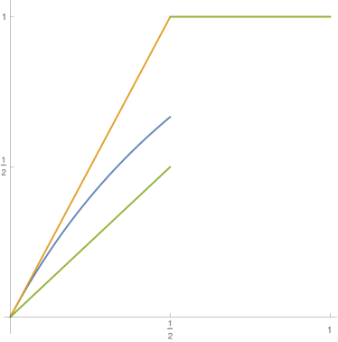
Figure 1. Graphs of $\varepsilon_{1\times n}(\delta)\leq\varepsilon_{{2\times 2}}(\delta)\leq(2\delta)\wedge 1$ in Proposition 1.1, for $\delta\in[0,1]$.

The bounds (1.6) and (1.9) were given in [Bur09, Theorem 14.1], [Pit14] and [Bur16, Theorem 18.1], while (1.7) and (1.8) are new. Our renewed interest in these results is prompted by

Claim 1.2.

[BP19] $\qquad\varepsilon_{{2\times 2}}(\delta)=\varepsilon_{\text{\rm finite}}(\delta)=\varepsilon(\delta)\qquad$ for all $\delta\in[0,1]$.

Proposition 1.1 implies that this identity holds with all values $0$ for $\delta=0$, and all values $1$ for $\delta\in[\mbox{$\frac{1}{2}$},1]$. The evaluations for $\delta\in[\mbox{$\frac{1}{2}$},1]$ come from the coherent $1\times 2$ distribution of $(X,Y)$ with equal probability $\frac{1}{2}$ at the points $(\mbox{$\frac{1}{2}$},0)$ and $(\mbox{$\frac{1}{2}$},1)\in[0,1]^{2}$. That is

$$X=E(Y)=\mbox{$\frac{1}{2}$}\mbox{ for }Y=B_{1/2}$$ (1.10)

where $B_{p}$ for $0\leq p\leq 1$ denotes a random variable with the Bernoulli$(p)$ distribution

$$P(B_{p}=1)=p P(B_{p}=0)=1-p$$ and . (1.11)

For $\delta\in(0,\mbox{$\frac{1}{2}$})$, Claim 1.2 is that equality holds in all the easy inequalities (1.6). The first of these equalities is proved here as (1.8). Equality in the second inequality of (1.6) for $\delta\in(0,\mbox{$\frac{1}{2}$})$ is much less obvious. The proof of this in [BP19] is at present quite long and difficult, by recursive reduction of $m$ and $n$ for $m\times n$ coherent $(X,Y)$, until the problem is reduced to the ${2\times 2}$ case treated here by (1.8). We hope this exposition of the easier evaluations in Proposition 1.1 might provoke someone to find a simpler proof of Claim 1.2.

Note from (1.7) and (1.8) that each of the functions $\varepsilon_{{1\times n}}$ and $\varepsilon_{{2\times 2}}$ is continuous on each of the intervals $[0,\mbox{$\frac{1}{2}$})$ and $[\mbox{$\frac{1}{2}$},1]$, but has an upward jump to $1$ at $\delta=\mbox{$\frac{1}{2}$}$, as shown in Figure 1. If Claim 1.2 is accepted for $\delta\in(0,\mbox{$\frac{1}{2}$})$, then $\varepsilon(\delta)$ too jumps up to $1$ at $\frac{1}{2}$.

Some further interpretations of these maximal probability functions, without assuming Claim 1.2, are presented in the following proposition, which is a specialization of Corollary 4.3 below. This involves the usual notion of stochastic ordering of real random variables $V$ and $W$, that is $V\leq_{d}W$ iff $P(V>x)\leq P(W>x)$ for all real $x$. This is well known to be equivalent to existence of a coupling of $V$ and $W$ on a common probability space with $P(V\leq W)=1$, and again to $Ef(V)\leq Ef(W)$ for all bounded increasing $f$.

Proposition 1.3.

The definition (1.5) of $\varepsilon(\delta)$ implies that for all coherent $(X,Y)$,

$$P(|X-Y|\geq 1-\delta)\leq\varepsilon(\delta)=P(\Delta\leq\delta)$$ (1.12)

for a random variable $\Delta$ with $0\leq\Delta\leq 1/2$. Moreover:

• For each $\delta\in[0,1]$ there is a coherent $(X,Y)$ which attains equality in (1.12).

• For all coherent $(X,Y)$, $|X-Y|\leq_{d}1-\Delta$. In particular, for $r>0$

$$E|X-Y|^{r}=\int_{0}^{1}ru^{r-1}P(|X-Y|\geq u)du\leq\int_{0}^{1}ru^{r-1}\varepsilon(1-u)du\leq\frac{2-2^{-r}}{1+r}.$$ (1.13)

For ${m\times n}$ coherent $(X,Y)$, the same conclusions hold, with the distribution of $\Delta_{{m\times n}}$ on $[0,\mbox{$\frac{1}{2}$}]$ defined by (1.12) with $\varepsilon_{{m\times n}}(\delta)$ in place of $\varepsilon(\delta)$.

The second inequality in (1.13) uses the upper bound in (1.9), followed by exact evaluation of the integral. Accepting Claim 1.2 gives a slightly smaller integral involving an incomplete beta function. For instance, for $r=1$ these upper bounds on $E|X-Y|$ are

$$0.75=\mbox{$\frac{3}{4}$}>\mbox{$\frac{3}{2}$}+\log 4-\log 9\approx 0.68907.$$

Corollary 2.5 shows that the supremum of $E|X-Y|$ over all coherent $(X,Y)$ is actually $\frac{1}{2}$.

The rest of this article is organized as follows. Section 2 recalls some background related to Proposition 1.1, which is proved in Section 3. Section 4 recalls some known characterizations of coherent distributions of $(X,Y)$. For reasons we do not understand well, these general characterizations seem to be of little help in establishing the evaluations of $\varepsilon(\delta)$ discussed above, or in settling a number of related problems about coherent distributions, which we present in Section 5. So much is left to be understood about the limitations on coherent opinions.

2. Background

Let $(X_{i},i\in I)$ be a finite collection of random variables defined on some common probability space $(\Omega,\mathcal{F},P)$, and suppose that each $X_{i}$ is the conditional expectation of some integrable random variable $X_{*}$ given some sub-$\sigma$-field $\mathcal{F}_{i}$ of $\mathcal{F}$:

$$X_{i}=E(X_{*}{\,|\,}\mathcal{F}_{i})\qquad(i\in I).$$ (2.1)

Doob’s well known bounds for tail probabilities and moments of the distributions of $\max_{i\in I}X_{i}$ and $\max_{i\in I}|X_{i}|$, for either an increasing or decreasing family of $\sigma$-fields, and extensions of these inequalities to families of $\sigma$-fields indexed by a directed set $I$, with suitable conditional independence conditions, play a central role in the theory of martingale convergence. See for instance [Kho02, HLOST16] and [Osȩ17] for recent refinements of Doob’s inequalities, and further references. For the diameter of a martingale

$$\max_{i,j\in I}|X_{i}-X_{j}|=\big{(}\max_{i\in I}X_{i}\big{)}+\big{(}-\max_{i\in I}(-X_{i})\big{)}\leq 2\max_{i\in I}|X_{i}|$$ (2.2)

there is no difficulty in bounding tail probabilities and moments, with an additional factor of $2$ to a suitable power. But finer results with best constants for the diameter have also been obtained in [DGM09, Osȩ15].

Much less is known about limitations on the distributions of such maximal variables for finite collections of $\sigma$-fields $(\mathcal{F}_{i},i\in I)$ without conditions of nesting or conditional independence. We focus here on joint distributions of $X_{i}=E(X_{*}{\,|\,}\mathcal{F}_{i})$ for $X_{*}$ with $0\leq X_{*}\leq 1$, and no restrictions except $\mathcal{F}_{i}\subseteq\mathcal{F}$ in a probability space $(\Omega,\mathcal{F},P)$. Setting $X_{J}:=E[X_{*}{\,|\,}\sigma(\cup_{i\in J}\mathcal{F}_{i})]$ makes $((X_{J},\mathcal{F}_{J}),J\subseteq I)$ a martingale indexed by subsets of $J$ of $I$, with $(X_{i},i\in I)$ the random vector of values of this martingale on singleton subsets of $I$. Assuming the basic probability space is sufficiently rich, there is a random variable $U$ with uniform distribution on $[0,1]$, with $U$ independent of $X_{*}$ and $\mathcal{F}_{I}$. Then $X_{*}$ can be be replaced by the indicator random variable $\mathds{1}(U\leq X_{*})$. So there is no loss of generality in supposing $X_{*}=\mathds{1}(A)$ is the indicator of some event $A$ with $P(A)=p\in[0,1]$. It follows that each $X_{i}$ is the conditional probability of $A$ given $\mathcal{F}_{i}$:

$$X_{i}=P(A{\,|\,}\mathcal{F}_{i})\mbox{ implying }EX_{i}\equiv p:=P(A)\qquad(i\in I).$$ (2.3)

Then either $(X_{i},i\in I)$ or its joint distribution on $[0,1]^{I}$ will be called coherent. Besides $EX=EY$, another necessary condition for a pair $(X,Y)$ to be coherent is provided by the following simplification and extension of [DDM95, Theorem 5.2]. See also Proposition 4.1 for some conditions that are both necessary and sufficient for $(X,Y)$ to be coherent.

Proposition 2.1.

Consider a pair of real-valued random variables $(X,Y)$ and assume that there exist disjoint intervals $G$ and $H$ and Borel sets $G^{\prime}\subseteq G$ and $H^{\prime}\subseteq H$ such that the events $(X\in G^{\prime})$ and $(Y\in H^{\prime})$ are almost surely identical, with $P(X\in G^{\prime})>0$. Then there is no integrable $Z$ with $X=E(Z{\,|\,}X)$ and $Y=E(Z{\,|\,}Y)$. In particular, this condition on $(X,Y)$ with values in $[0,1]^{2}$ implies that $(X,Y)$ is not coherent.

Proof.

Suppose that $G^{\prime}\subseteq G$ and $H^{\prime}\subseteq H$. If $X=E(Z{\,|\,}X)$ and $Y=E(Z{\,|\,}Y)$ for some integrable $Z$ then it is easily seen that

$$G\ni E(Z{\,|\,}X\in G^{\prime})=E(Z{\,|\,}Y\in H^{\prime})\in H,$$ (2.4)

where $E(Z{\,|\,}B)$ denotes $E(Z\mathds{1}_{B})/P(B)$ for any $B$ with $P(B)>0$. Since $G\cap H=\emptyset$, we obtain the conclusion. ∎

For disjoint intervals $G^{\prime}=G=[0,a)$ and $H^{\prime}=H=(b,1]$, Proposition 2.1 yields:

Corollary 2.2.

If $X-a$ and $Y-b$ are sure to be of opposite sign for some $0\leq a\leq b\leq 1$:

$$P((X-a)(Y-b)<0)=1,$$ (2.5)

and $P(Y>b)>0$, then the distribution of $(X,Y)$ is not coherent.

This corrects the claim above [DDM95, Theorem 5.2] that (2.5) alone makes $(X,Y)$ not coherent. (This is false if $P(Y>b)=0$; take $a=\mbox{$\frac{1}{4}$},b=\mbox{$\frac{3}{4}$}$ and $X=Y=\mbox{$\frac{1}{2}$}$).

The following construction of a coherent distribution of $n$ variables $(X_{1},\ldots,X_{n})$ was used in [DP80a] to build counterexamples in the theory of almost sure convergence of martingales relative to directed sets.

Example 2.3.

(The $(n,p)$-daisy, with $n$ petals and a Bernoulli$(p)$ center) [DP80a]. Let $A,A_{1},\ldots,A_{n}$ be a measurable partition of $\Omega$ with

$$P(A)=p\mbox{ and }P(A_{i})=\frac{1-p}{n}\mbox{ for }1\leq i\leq n.$$

For $1\leq i\leq n$ let $\mathcal{F}_{i}$ be the $\sigma$-field generated by $A\cup A_{i}$. Then set

$$X_{i}:=P(A{\,|\,}\mathcal{F}_{i})=p_{n}\mathds{1}(A\cup A_{i})\mbox{ with }p_{n}:=\frac{np}{np-p+1}.$$ (2.6)

To explain the daisy mnemonic, imagine $\Omega$ is the union of $n+1$ parts of a daisy flower, with center $A$ of area $p$, surrounded by $n$ petals $A_{i}$ of equal areas, with total petal area $1-p$. For each petal $A_{i}$, an $i$th petal observer learns whether or not a point picked at random from the daisy area has fallen in (the center $A$ or their petal $A_{i}$), or in some other petal. Each petal observer’s conditional probability $X_{i}$ of $A$ is then as in (2.6). The sequence of $n$ variables $(X_{1},\ldots,X_{n})$ is both coherent  and exchangeable, with constant expectation $p$:

• given $A$ the sequence $(X_{1},\ldots,X_{n})$ is identically equal to the constant $p_{n}$;

• given the complement $A^{c}$, the sequence $(X_{1},\ldots,X_{n})$ is $p_{n}$ times an indicator sequence with a single $1$ at a uniformly distributed index in $\{1,\ldots,n\}$.

The $(n,p)$-daisy example was designed to make $\max_{1\leq i\leq n}X_{i}=p_{n}$, a constant, as large as possible with $EX_{i}\equiv p$. As observed in [DP80b, p.224], this $p_{n}$ is the largest possible essential infimum of values of $\max_{i}X_{i}$ for any coherent distribution of $(X_{1},\ldots,X_{n})$ with $EX_{i}\equiv p$. This special property involves the $n$-petal daisy in the solution in various extremal problems for coherent opinions. For instance, $(X,Y)=(X_{1},X_{2})$ derived from the $(2,p)$ daisy with $p=(1-\delta)/(1+\delta)$, so $p_{2}=1-\delta$, is the coherent pair in (1.4). This provides the lower bound for $\varepsilon_{{2\times 2}}(\delta)$ in (1.6), which according to (1.8) is attained with equality for $\delta\in[0,\mbox{$\frac{1}{2}$})$. Also:

Proposition 2.4.

[DP80b] For every coherent distribution of $(X_{i},1\leq i\leq n)$ with $EX_{i}\equiv p$,

$$E\max_{1\leq i\leq n}X_{i}\leq\frac{p(n-p)}{1+p(n-2)}.$$ (2.7)

Moreover, this bound is attained by taking $(X_{1},\ldots,X_{n-1})$ to be the $(n-1,p)$-daisy sequence, and $X_{n}=\mathds{1}_{A}$, the Bernoulli$(p)$ indicator of the daisy center.

For example, if $(X_{1},\ldots,X_{n})$ is the $(n,p)$ daisy sequence, the left hand side of (2.7) is $p_{n}$ in (2.6), which is strictly less than the right side of (2.7). Proposition 2.4 implies:

Corollary 2.5.

For every coherent distribution of $(X,Y)$ on $[0,1]^{2}$ with $EX=EY=p$,

$$E|X-Y|\leq 2p(1-p)\leq\mbox{$\frac{1}{2}$}$$ (2.8)

with equality in the first inequality if $X=p$ and $Y\stackrel{{\scriptstyle d}}{{=}}B_{p}$ as in (1.11).

Proof.

Take $n=2$ in (2.7) and use $|X-Y|=2(X\vee Y)-X-Y$. ∎

As noted below Proposition 1.3, the bound (2.8) is better than what is obtained by integration of the least upper bounds (1.5) on tail probabilities of $|X-Y|$. Combine (2.8) with Markov’s inequality to see that

$$P(|X-Y|\geq 1-\delta)\leq\frac{2p(1-p)}{(1-\delta)}\leq\frac{1}{2(1-\delta)}.$$ (2.9)

But without restricting $p$ to be close to $0$ or $1$, this does not reduce the upper bound of (1.12). See also Problems 5.3 and 5.4.

3. Proof of Proposition 1.1

The evaluation (1.7) in Proposition 1.1 is implied by Lemma 3.1 for $\delta\in[0,\mbox{$\frac{1}{2}$})$ and by example (1.10) for $\delta\in[\mbox{$\frac{1}{2}$},1]$.

Lemma 3.1.

If $X=E(Y{\,|\,}X)$ and $0\leq Y\leq 1$ then $P(|Y-X|\geq 1-\delta)\leq\delta\mbox{ for }\delta\in[0,\mbox{$\frac{1}{2}$})$, with equality if $X=\delta$ and $Y=B_{\delta}$.

Proof.

Suppose $X=p$ is constant and $Y=Y_{p}\in[0,1]$ has $EY_{p}=p$. By consideration of $Y_{1-p}=1-Y_{p}$ it can be supposed that $p\in[0,\mbox{$\frac{1}{2}$}]$. But then for $\delta\in[0,\mbox{$\frac{1}{2}$})$

$$|Y_{p}-p|\geq 1-\delta\mbox{ iff }Y_{p}\geq 1-\delta+p,$$

so Markov’s inequality gives

$$P(|Y_{p}-p|\geq 1-\delta)\leq\frac{p\,\mathds{1}(p\leq\delta)}{1-\delta+p}\leq\delta\mbox{ for }0\leq p\leq\mbox{$\frac{1}{2}$}\mbox{ and }0\leq\delta<\mbox{$\frac{1}{2}$}.$$ (3.1)

The more general assertion of the lemma follows by conditioning on $X$. ∎

Turning to consideration of (1.8), we start with a lemma of independent interest, which controls the variability of $P(A{\,|\,}G)$ as a function of $G$ with $P(G)>0$ by a bound that does not depend on $A$. We work here with the elementary conditional probability which is the number $P(A{\,|\,}G):=P(AG)/P(G)$ rather than a random variable. Let $G\triangle H:=GH^{c}\cup G^{c}H$ denote the symmetric difference of $G$ and $H$.

Lemma 3.2.

For events $A$, $G$ and $H$ with $P(G)>0$ and $P(H)>0$,

$$|P(A{\,|\,}G)-P(A{\,|\,}H)|\leq P(G\triangle H{\,|\,}G\cup H)=1-\frac{P(GH)}{P(G)+P(H)-P(GH)}.$$ (3.2)

Consequently, for each $0\leq\delta\leq 1$,

$$|P(A{\,|\,}G)-P(A{\,|\,}H)|\geq 1-\delta\implies P(GH)\leq\frac{\delta}{(1+\delta)}(P(G)+P(H)).$$ (3.3)

Proof.

Let $p=P(GH^{c}),q=P(GH),r=P(G^{c}H)$ and $a=P(A{\,|\,}GH^{c}),b=P(A{\,|\,}GH),c=P(A{\,|\,}G^{c}H)$, with the convention that $a=0$ if $P(GH^{c})=0$, and a similar convention for $b$ and $c$. Then

$$P(A{\,|\,}G)-P(A{\,|\,}H)=\frac{pa+qb}{p+q}-\frac{qb+rc}{q+r}\leq\frac{p+r}{p+q+r}$$ (3.4)

from which (3.2)-(3.3) follow easily. To check the inequality in (3.4), observe that for fixed $p,q,r$ the difference of fractions in the middle is obviously maximized by taking $a=1,c=0$. That done, the difference is a linear function of $b$, whose maximum over $0\leq b\leq 1$ is attained either at $b=0$ or at $b=1$, when the inequality is obvious. ∎

It is easily checked that for $p,q,r$ as above, with $p+q>0$ and $q+r>0$, there is equality in (3.4) iff one of the following three conditions holds, where in each case the condition on $G$, $H$, and $A$ should be understood modulo events of probability $0$:

• either $p>0,q=0,r>0,a=1,b=c=0$, meaning $G\cap H=\emptyset$ and $A=G$;

• or $p=0,q>0,r>0,a=0,b=1,c=0$, meaning $G\subseteq H$ and $A=G$;

• or $p>0,q>0,r=0,a=1,b=c=0$, meaning $H\subseteq G$ and $A=GH^{c}$.

Consequently, there is equality in (3.2) iff one of these three conditions holds, either exactly as above or with $G$ and $H$ switched.

Lemma 3.3.

Suppose that $X=P(A{\,|\,}X)$ and $Y=P(A{\,|\,}Y)$ have discrete distributions. Fix $0<\delta<1/2$, and suppose that for each pair of possible $(x,y)$ of $(X,Y)$ with $|y-x|\geq 1-\delta$ there is no other such pair $(x^{\prime},y^{\prime})$ with either $x^{\prime}=x$ or $y^{\prime}=y$. Then

$$P(|Y-X|\geq 1-\delta)\leq\frac{2\delta}{1+\delta}\qquad(0<\delta<1/2).$$ (3.5)

Proof.

Application of (3.3) gives for each pair $(x,y)$ with $|y-x|\geq 1-\delta$

$$P(X=x,Y=y)\leq\frac{\delta}{1+\delta}\left(P(X=x)+P(Y=y)\right).$$ (3.6)

The assumption is that as $(x,y)$ ranges over pairs $(x,y)$ with $|y-x|\geq 1-\delta$, the events $(X=x)$ are disjoint, and so are the events $(Y=y)$. So (3.5) follows by summation of (3.6) over such $(x,y)$. ∎

Proof of (1.8).

In view of (1.7), and the examples (1.10) and (1.4), it is enough to establish (3.5) for ${2\times 2}$ coherent $(X,Y)$ whose possible values are contained in the $4$ corners of a rectangle $R:=[x_{1},x_{2}]\times[y_{1},y_{2}]\subseteq[0,1]^{2}$ with $x_{1}<x_{2}$ and $y_{1}<y_{2}$. Fix $0<\delta<\mbox{$\frac{1}{2}$}$. Then $\{(x,y):|y-x|\geq 1-\delta\}=T\cup T^{\prime}$ for right triangles $T$ and $T^{\prime}$ in the upper left and lower right corners of $[0,1]^{2}$. If neither $T$ nor $T^{\prime}$ contains two corners on the same side of $R$, then (3.5) holds by the above lemma. Otherwise, by the reflection symmetries (1.3), it is enough to discuss the case when $T$ contains the two left corners of $R$. Then $T$ contains no more corners of $R$; for that would make

$$(EX,EY)\in\{(p,p),0\leq p\leq 1\}\cap([0,\delta]\times[1-\delta,1])=\emptyset\mbox{ by }\delta<\mbox{$\frac{1}{2}$}.$$

Finally, for $R$ with two left corners in $T$ and two right corners not in $T\cup T^{\prime}$, replacing $(X,Y)$ by $(X,EY)$ gives a $2\times 1$ example with the same $P(|X-Y|\geq 1-\delta)$, which is at most $\delta$ by (1.7). ∎

Proof of (1.9).

This argument from [Pit14] was presented in [Bur16, Theorem 18.1], but is included here for the reader’s convenience. The lower bound in (1.9) is obvious from (1.6). For the upper bound, it is enough to discuss the case $\delta\in[0,\mbox{$\frac{1}{2}$})$. Observe that

$$(|X-Y|\geq 1-\delta)\subseteq(X\leq\delta,Y\geq 1-\delta)\cup(Y\leq\delta,X\geq 1-\delta).$$ (3.7)

But since $X=P(A{\,|\,}X)$ and $1-Y=P(A^{c}{\,|\,}Y)$,

$$P(X\leq\delta,Y\geq 1-\delta,A) \leq P(X\leq\delta,A)=E\mathds{1}(X\leq\delta)X\leq\delta P(X\leq\delta),$$

$$P(X\leq\delta,Y\geq 1-\delta,A^{c}) \leq P(Y\geq 1-\delta,A^{c})=E\mathds{1}(1-Y\leq\delta)(1-Y))\leq\delta P(Y\geq 1-\delta).$$

It follows that

$$P(X\leq\delta,Y\geq 1-\delta) \leq \delta[P(X\leq\delta)+P(Y\geq 1-\delta)],$$ (3.8)

$$P(Y\leq\delta,X\geq 1-\delta) \leq \delta[P(Y\leq\delta)+P(X\geq 1-\delta)].$$ (3.9)

For $\delta<1/2$ the events $(X\leq\delta)$ and $(X\geq 1-\delta)$ are disjoint, so $P(X\leq\delta)+P(X\geq 1-\delta)\leq 1$, and the same for $Y$. Add (3.8) and (3.9) and use (3.7) to obtain the upper bound in (1.9). ∎

4. Coherent distributions

The following proposition summarizes a number of known characterizations of the set of coherent distributions of $(X,Y)$, due to [DP80b], [GKRS91] and [DDM95].

Proposition 4.1.

Let $(X,Y)$ be a pair of random variables defined on a probability space $(\Omega,\mathcal{F},P)$, on which there is also defined a random variable $U$ with uniform distribution, independent of $(X,Y)$. Then the following conditions are equivalent:

• The joint law of $(X,Y)$ is coherent.

• There exists a random variable $Z$ defined on $(\Omega,\mathcal{F},P)$, with $0\leq Z\leq 1$, such that both

  $$E[Zg(X)]=E[Xg(X)]\quad\mbox{ and }\quad E[Zg(Y)]=E[Yg(Y)]$$ (4.1)

  either for all bounded measurable functions $g$ with domain $[0,1]$, or for all bounded continuous functions $g$.

• There exists a measurable function $\phi:[0,1]^{2}\mapsto[0,1]$ such that

  $$E[\phi(X,Y)g(X)]=E[Xg(X)]\quad\mbox{ and }\quad E[\phi(X,Y)g(Y)]=E[Yg(Y)]$$ (4.2)

  either for all bounded measurable $g$, or for all bounded continuous $g$.

• $EX=EY=p$ for some $0\leq p\leq 1$, and

  $$E\big{[}X\mathds{1}(X\in B)\big{]}+E\big{[}Y\mathds{1}(Y\in C)\big{]}\leq p+P(X\in B,Y\in C)$$ (4.3)

  for all $B,C\in\mathcal{B}$, where $\mathcal{B}$ may be either the collection of all Borel subsets of $[0,1]$, or the collection of all finite unions of intervals contained in $[0,1]$.

Proof.

Condition (i) is just (ii) for $Z$ an indicator variable, while (ii) for $0\leq Z\leq 1$ implies (iii) for $\phi(X,Y)=E(Z{\,|\,}X,Y)$. Assuming (iii), (ii) holds with $Z=\mathds{1}(U\leq\phi(X,Y))$ for the uniform $[0,1]$ variable $U$ independent of $(X,Y)$. So (i), (ii) and (iii) are equivalent. The equivalence of (iii) and (iv) is an instance of [Str65, Theorem 6], according to which for any finite measure $m$ on $[0,1]^{2}$, a pair of probability distributions $Q$ and $R$ on $[0,1]$ are the marginals of the measure $\phi(x,y)m(dx\,dy)$ on $[0,1]^{2}$, for $\phi$ a product measurable function with $0\leq\phi\leq 1$, iff

$$Q(B)+R(C)\leq 1+m(B\times C)$$

for all Borel sets $B$ and $C$. This is equivalent to the same condition for all finite unions of intervals, by elementary measure theory. After dismissing the trivial case $p=0$, this result is applied here to $m(\cdot)=P((X,Y)\in\cdot)/p$ for $X$ and $Y$ with mean $p$, with $Q(B):=E\left[X\mathds{1}(X\in B)\right]/p$ and $R(C):=E\left[Y\mathds{1}(Y\in C)\right]/p$. ∎

The characterizations (ii) and (iii) above extend easily to a coherent family $(X_{i},i\in I)$, while (iv) does not [DDM95, p. 288].

Corollary 4.2.

[DP80b] For any finite $I$, the set of coherent distributions of $(X_{i},i\in I)$ is a convex, compact subset of probability distributions on $[0,1]^{I}$ with the usual weak topology.

Proof.

To check convexity, suppose that $(X_{i},i\in I)$ is subject to the extension of (4.1). That is for some additional index $*\notin I$ and $X_{*}=Z\in[0,1]$,

$$E[X_{*}g(X_{i})]=E[X_{i}g(X_{i})]\mbox{ for all bounded continuous }g\mbox{ and }i\in I,$$ (4.4)

and the same for $Y=(Y_{i},i\in I_{*})$ instead of $X$, with $I_{*}:=I\cup\{*\}$. Construct these random vectors $X$ and $Y$ on a common probability space with a Bernoulli$(p)$ variable $B_{p}$, with $X,Y$ and $B_{p}$ independent. Let $W:=B_{p}X+(1-B_{p})Y$, so the law of $W$ is the mixture of laws of $X$ and $Y$ with weights $p$ and $1-p$. Then (4.4) for $X$ and $Y$ implies (4.4) for $W$. The proof of sequential compactness is similar. Define $X$ to be a subsequential limit in distribution of some sequence of random vectors $X_{n}:=(X_{n,i},i\in I_{*})$ subject to (4.4) for each $n$, to deduce (4.4) for $X$ by bounded convergence. ∎

Corollary 4.3.

Let $\mathcal{C}$ be a non-empty set of distributions of $X=(X_{i},i\in I)$ on $\mathbb{R}^{I}$ that is compact in the topology of weak convergence, such as coherent distributions of $X$ on $[0,1]^{I}$. Let $G(x):=\sup_{\mathcal{C}}P(g(X)\leq x)$ for some particular continuous function $g$, and $x\in\mathbb{R}$, where the $\sup_{\mathcal{C}}$ is over $X$ with a distribution in $\mathcal{C}$. Then

• for each fixed $x\in\mathbb{R}$ there exists a distribution of $X$ in $\mathcal{C}$ with $G(x)=P(g(X)\leq x)$;

• $G(x)=P(\gamma\leq x)$ is the cumulative distribution function of a random variable $\gamma$ which is stochastically smaller than $g(X)$ for every distribution of $X$ in $\mathcal{C}$: $\gamma\leq_{d}g(X)$.

Proof.

By definition of $G(x)$, for each fixed $x$ there exists a sequence of random vectors $X_{n}$ with distributions in $\mathcal{C}$ such that $F_{n}(x):=P(g(X_{n})\leq x)\uparrow G(x)$. By compactness of $\mathcal{C}$, it may be supposed that $X_{n}\stackrel{{\scriptstyle d}}{{\to}}X$, meaning the distribution of $X_{n}$ converges to that of some $X\in\mathcal{C}$. That implies $g(X_{n})\stackrel{{\scriptstyle d}}{{\to}}g(X)$. Let $F(x):=P(g(X)\leq x)$. Since $F_{n}(x)$ and $F(x)$ are the probabilities assigned by the laws of $g(X_{n})$ and $g(X)$ to the closed set $(-\infty,x]$, [Bil95, Theorem 29.1] gives

$$G(x)\geq F(x)\geq\limsup_{n}F_{n}(x)=G(x).$$

For (ii), the only property of a cumulative distribution function that is not an obvious property of $G$ is right continuity. To see this, take $x_{n}\downarrow x$ and $X_{n}$ with $P(g(X_{n})\leq x)=F_{n}(x)$ such that $F_{n}(x_{n})=G(x_{n})$, and $X_{n}\stackrel{{\scriptstyle d}}{{\to}}X$ with distribution in $\mathcal{C}$. Let $F(x):=P(g(X)\leq x)$. Then for each fixed $m$, by the same result of [Bil95],

$$F(x_{m})\geq\limsup_{n}F_{n}(x_{m})\geq\limsup_{n}F_{n}(x_{n})=\limsup_{n}G(x_{n})=G(x+).$$

Finally, letting $m\to\infty$ gives $G(x)\geq F(x)=F(x+)\geq G(x+)\geq G(x)$. ∎

Returning to discussion of a just pair random variables $(X,Y)$ with values in $[0,1]^{2}$, as in Proposition 4.1, suppose further that $X$ and $Y$ are independent, with $EX=EY=p$. Then the inequality (4.3) becomes

$$EX\mathds{1}(X\in B)+EY\mathds{1}(Y\in C)\leq p+P(X\in B)P(Y\in C).$$ (4.5)

It was shown in [GKRS91, Theorem 4] that this condition, just for $B=(s,1]$ and $C=(t,1]$ for $0\leq s,t\leq 1$, characterizes all possible pairs of marginal distributions on $[0,1]$ of independent $X$ and $Y$ with mean $p$ such that $(X,Y)$ is coherent. See also [Lau03, Proposition 3].

5. Open problems

Problem 5.1.

Give a simple proof of Claim 1.2.

A check on this claim is to try to confirm it first with additional assumptions, such as independence of $X$ and $Y$, using (4.5). But this does not seem easy. It leads rather to:

Conjecture 5.2.

If $(X,Y)$ is coherent, and $X$ and $Y$ are independent, then

$$P(|X-Y|\geq 1-\delta)\leq 2\delta(1-\delta)\qquad\text{ for }\delta\in[0,\mbox{$\frac{1}{2}$}).$$ (5.1)

Equality is attained in (5.1) for independent $X$ and $Y$ with

$$X\stackrel{{\scriptstyle d}}{{=}}Y\stackrel{{\scriptstyle d}}{{=}}(1-\delta)B_{1-\delta} A=(X=Y=1-\delta)$$ and . (5.2)

The method of proof of (1.8) establishes (5.1) for ${2\times 2}$ laws of $(X,Y)$. But like Claim 1.2, the extension of (5.1) to general distributions of $X$ and $Y$ seems quite challenging.

The problems solved by (1.8) for $t(X,Y)=1(|X-Y|\geq 1-\delta)$ and by the case $n=2$ of (2.7) for $t(X,Y)=X\vee Y$, are instances of the following more general problem, with further variants as above, assuming $X$ and $Y$ are independent.

Problem 5.3.

[DP80b, p.224] Given some target function $t(X,Y)$ defined on $[0,1]^{2}$, evaluate $\sup_{\mathcal{C}}Et(X,Y)$, the supremum of $Et(X,Y)$ as the law of $(X,Y)$ ranges over the set $\mathcal{C}$ of coherent laws on $[0,1]^{2}$. Or the same for $\mathcal{C}(p)$, coherent laws of $(X,Y)$ with $EX=EY=p$.

This problem seems to be open even for $XY$, or $|X-Y|^{r}$ for $r\neq 1$, when (1.13) gives only a crude upper bound. Another instance of this problem is to evaluate

$$\varepsilon(\delta,p):=\sup_{\mathcal{C}(p)}P(|X-Y|\geq 1-\delta).$$ (5.3)

For each $\delta\in(0,1)$, examples of coherent $(X,Y)$ with

$$P(|X-Y|\geq 1-\delta)=p(\delta):=2\delta/(1+\delta)$$ (5.4)

are the ${2\times 2}$ example (1.4), say $(X_{\delta},Y_{\delta})$, its reflection $(1-X_{\delta},1-Y_{\delta})$, and any mixture of these two laws, which is a $4\times 4$ law in $\mathcal{C}(p)$ for $p$ between $p(\delta)$ and $1-p(\delta)$. So

$$p(\delta)\leq\varepsilon(\delta,p)\leq\varepsilon(\delta)\mbox{ for }p\mbox{ between }p(\delta)\mbox{ and }1-p(\delta).$$ (5.5)

If Claim 1.2 is accepted, both inequalities are equalities for $\delta\in(0,\mbox{$\frac{1}{2}$}]$. But that leaves open:

Problem 5.4.

Find $\varepsilon(\delta,p)$ for $\delta\in(0,\mbox{$\frac{1}{2}$}]$, and $p$ not covered by (5.5).

For a bounded upper semicontinuous $t$, such as the indicator of a closed set, the $\sup_{\mathcal{C}}Et(X,Y)$ will be attained at a distribution of $(X,Y)$ in ${\text{\rm ext}}(\mathcal{C})$, the set of extreme points of the compact, convex set $\mathcal{C}$ of coherent distributions [BS91]. This leads to:

Problem 5.5.

[DP80b, p.224] [DDM95, p.273]. Characterize ${\text{\rm ext}}(\mathcal{C})$.

For the particular target functions $t$ involved in (2.7) and in Claim 1.2, the $\sup_{\mathcal{C}}Et(X,Y)$ is attained by $2\times 2$ distributions of $(X,Y)$. Hence the following:

Conjecture 5.6.

Every extreme coherent law of $(X,Y)$ is a $2\times 2$ law.

Let $\mathcal{M}$ be the convex, compact subset of $\mathcal{C}$ comprising laws of two term martingales $(X,Y)$, with $X=E(Y{\,|\,}X)$, $Y\in[0,1]$. It is elementary and well known that ${\text{\rm ext}}(\mathcal{M})$ is the set of $1\times 2$ laws of $(p,Y_{p})$ for two-valued $Y_{p}\in[0,1]$ with $E(Y_{p})=p$. But the extension of this result conjectured above does not seem obvious. It may be relatively easy to settle whether or not every extreme $m\times n$ coherent $(X,Y)$ is actually $2\times 2$, for some small $m$ and $n$. In view of (4.3), for any particular $t$, the evaluation of $\sup_{\mathcal{C}}Et(X,Y)$, with restriction to a fixed set of $m$ values for $X$ and $n$ values for $Y$, is a linear programming problem, with a finite number of constraints depending on the given values. This problem may be solved by modern programming techniques, at least for small $m$ and $n$. By solving such $2\times 3$ problems, a solution might be found which is not attained by any $2\times 2$ coherent law. Then Conjecture 5.6 would be false. On the other hand, if Conjecture 5.6 is true, that would increase interest in the structure of $2\times 2$ extreme laws. The following proposition is easily proved using (4.3):

Proposition 5.7.

For each a rectangle $R=[x_{1},x_{2}]\times[y_{1},y_{2}]\subseteq[0,1]^{2}$, let $\mathcal{C}_{{2\times 2}}(R)$ denote the set of coherent laws of $(X,Y)$ on the corners of $R$. Then

• $\mathcal{C}_{{2\times 2}}(R)$ is non-empty iff $R$ intersects the diagonal $\{(p,p),0\leq p\leq 1\}$, that is iff $x_{1}\vee y_{1}\leq x_{2}\wedge y_{2}$.

• If $x_{1}\vee y_{1}=x_{2}\wedge y_{2}=p$, then $(p,p)$ is a corner of $R$, and the unique law in $\mathcal{C}_{{2\times 2}}(R)$ is degenerate with $X=Y=p$.

• If $x_{1}\vee y_{1}<x_{2}\wedge y_{2}$, the set ${\text{\rm ext}}\,\mathcal{C}_{{2\times 2}}(R)$ of extreme points of the convex set $\mathcal{C}_{{2\times 2}}(R)$ is identical to the set of all extreme coherent laws supported by the set of corners of $R$. This set of laws ${\text{\rm ext}}\,\mathcal{C}_{{2\times 2}}(R)$ forms a convex polygon in a $2$-dimensional affine subspace of the set of probability distributions on those corners, with at least $2$ and at most $8$ vertices.

Examples show that the number of vertices of this polygon varies as a function of the rectangle $R$, from $2$ if $R$ is pushed into a corner of $[0,1]^{2}$, to at least $6$ for some more central locations. Regardless of the status of Conjecture 5.6, this leads to:

Problem 5.8.

Provide an accounting of the extreme $2\times 2$ coherent laws of $(X,Y)$ which is adequate to recover (1.8) and (2.8), and to find the extrema of $Et(X,Y)$ over $2\times 2$ coherent laws for other functions $t$, such as $t(X,Y)=XY$ or $|X-Y|^{r}$ for $r>0$.

Problem 5.9.

Extensions of above problems to $n>2$ coherent opinions.

6. Acknowledgments

We are grateful to David Aldous and Soumik Pal for very helpful advice.

References

• [Bil95] Patrick Billingsley. Probability and measure. Wiley Series in Probability and Mathematical Statistics. John Wiley & Sons, Inc., New York, third edition, 1995. A Wiley-Interscience Publication.
• [BP19] Krzysztof Burdzy and Soumik Pal. Contradictory predictions. (forthcoming), 2019.
• [BS91] Viktor Benes and Josef Stepan. Extremal solutions in the marginal problem. In Advances in Probability Distributions with Given Marginals, pages 189–206. Springer, 1991.
• [Bur09] Krzysztof Burdzy. The search for certainty. On the clash of science and philosophy of probability. World Scientific Publishing Co. Pte. Ltd., Hackensack, NJ, 2009.
• [Bur16] Krzysztof Burdzy. Resonanceβ€”from probability to epistemology and back. Imperial College Press, London, 2016.
• [DDM95] A.Β P. Dawid, M.Β H. DeGroot, and J.Β Mortera. Coherent combination of experts’ opinions. Test, 4(2):263–313, Dec 1995.
• [DGM09] LesterΒ E. Dubins, David Gilat, and Isaac Meilijson. On the expected diameter of an $L_{2}$-bounded martingale. Ann. Probab., 37(1):393–402, 2009.
• [DP80a] LesterΒ E. Dubins and Jim Pitman. A divergent, two-parameter, bounded martingale. Proc. Amer. Math. Soc., 78(3):414–416, 1980.
• [DP80b] LesterΒ E. Dubins and Jim Pitman. A maximal inequality for skew fields. Z. Wahrsch. Verw. Gebiete, 52(3):219–227, 1980.
• [GKRS91] Sam Gutmann, J.Β H.Β B. Kemperman, J.Β A. Reeds, and L.Β A. Shepp. Existence of probability measures with given marginals. Ann. Probab., 19(4):1781–1797, 1991.
• [HLOST16] Pierre Henry-LabordΓ¨re, Jan ObΕ‚Γ³j, Peter Spoida, and Nizar Touzi. The maximum maximum of a martingale with given $n$ marginals. Ann. Appl. Probab., 26(1):1–44, 2016.
• [Kho02] Davar Khoshnevisan. Multiparameter processes. Springer Monographs in Mathematics. Springer-Verlag, New York, 2002. An introduction to random fields.
• [Lau03] SteffenΒ L. Lauritzen. Rasch models with exchangeable rows and columns. In Bayesian statistics, 7 (Tenerife, 2002), pages 215–232. Oxford Univ. Press, New York, 2003.
• [OsΘ©15] Adam OsΘ©kowski. Estimates for the diameter of a martingale. Stochastics, 87(2):235–256, 2015.
• [OsΘ©17] Adam OsΘ©kowski. Method of moments and sharp inequalities for martingales. In Inequalities and extremal problems in probability and statistics, pages 1–27. Academic Press, London, 2017.
• [Pit14] Jim Pitman. Bounds on the probability of radically different opinions. Unpublished, 2014.
• [Str65] Volker Strassen. The existence of probability measures with given marginals. The Annals of Mathematical Statistics, 36(2):423–439, 1965.