11institutetext: University of Illinois at Urbana-Champaign 11email: {cx2,sanmi,indy}@illinois.edu

SLSGD: Secure and Efficient Distributed On-device Machine Learning

Cong Xie 11    Sanmi Koyejo 11    Indranil Gupta 11
Abstract

We consider distributed on-device learning with limited communication and security requirements. We propose a new robust distributed optimization algorithm with efficient communication and attack tolerance. The proposed algorithm has provable convergence and robustness under non-IID settings. Empirical results show that the proposed algorithm stabilizes the convergence and tolerates data poisoning on a small number of workers.

Keywords:
Distributed SGD.

1 Introduction

Edge devices/IoT such as smart phones, wearable devices, sensors, and smart homes are increasingly generating massive, diverse, and private data. In response, there is a trend towards moving computation, including the training of machine-learning models, from cloud/datacenters to edge devices [1, 24]. Ideally, since trained on massive representative data, the resulting models exhibit improved generalization. In this paper, we consider distributed on-device machine learning. The distributed system is a server-worker architecture. The workers are placed on edge devices, which train the models on the private data. The servers are placed on the cloud/datacenters which maintain a shared global model. Distributed settings require addressing some novel engineering challenges, including the following:

  • Limited, heterogeneous computation. Edge devices, including smart phones, wearable devices, sensors, or vehicles typically have weaker computational ability, compared to the workstations or datacenters used in typical distributed machine learning. Thus, simpler models and stochastic training are usually applied in practice. Furthermore, different devices have different computation capabilities.

  • Limited communication The connection to the central servers are not guaranteed. Communication can be frequently unavailable, slow, or expensive (in money or in the power of battery). Thus, frequent high-speed communication is typically unaffordable.

  • Decentralized, non-IID training data. Privacy needs and legal requirements (e.g., US HIPAA laws [12] in a smart hospital, or Europe’s GDPR law [8]) may necessitate that training be performed on-premises using IoT devices and edge machines, and that data and models must not be deposited in the cloud or cloudlets. In more general cases, the users simply dislike sharing their on-device data which potentially reveals private information. As a result, the data distribution on different devices are neither mixed nor IID i.e. unlike standard settings, device data are non-identically distributed samples from the population. This is particularly true when each device is controlled by a specific user whose behavior is supposed to be unique. Furthermore, the sampled data on nearby devices are potentially non-independent, since such devices can be shared by the same user or family. For example, the data of a step counter from a wearable fitness tracker and a smart phone owned by the same user can have different distributions of motion data with mutual dependency. Imagine that the fitness tracker is only used when the user is running, and the smart phone is only used when the user is walking, which results in different distributions. On the other hand, the complementation yields dependency.

  • Untrusted workers and data poisoning. The servers have limited control over the users’ behavior. To protect the privacy, the users are in general anonymous to the servers. Although it is possible to verity the identity of workers/devices [25], nefarious users can feed poisoned data with abnormal behaviors without backdooring OS. As a result, some workers may push models learned on poisoned data to the servers.

To overcome the challenges above, we introduce Secure Local Stochastic Gradient Descent (SLSGD), which reduces the communication overhead with local updates, and secures the global model against nefarious users and poisoned data. We summarize the key properties of SLSGD below:

  • Local SGD. SGD is widely used for training models with lower computation overhead. To reduce communication overhead, we use SGD with local updates. The workers do not synchronize with the server after each local gradient descent step. After several local iterations, the workers push the updated model to the servers, which is different from the traditional distributed synchronous SGD where gradients are pushed in each local gradient descent step. To further reduce the communication overhead, the training tasks are activated on a random subset of workers in each global epoch.

  • Secure aggregation. In each global epoch, the servers send the latest global model to the activated workers, and aggregate the updated local models. In such procedure, there are two types of threats: i) poisoned models pushed from comprised devices, occupied or hacked by nefarious users; ii) accumulative error, variance, or models over-fitted on the local dataset, caused by infrequent synchronization of local SGD. To secure the global model against these two threats, we use robust aggregation which tolerates abnormal models, and moving average which mitigates the errors caused by infrequent synchronization.

To our knowledge, there is limited work on local SGD with theoretical guarantees [29, 26]. The existing convergence guarantees are based on the strong assumption of IID training data or homogeneous local iterations, which we have argued is inappropriate for distributed learning on edge devices.

We propose SLSGD, which is a variant of local SGD with provable convergence under non-IID and heterogeneous settings, and tolerance to nefarious users. In summary, the main contributions are listed as follows:

  • We show that SLSGD theoretically converges to global optimums for strongly convex functions, non-strongly convex functions, and a restricted family of non-convex functions, under non-IID settings. Furthermore, more local iterations accelerate the convergence.

  • We show that SLSGD tolerates a small number of workers training on poisoned data. As far as we know, this paper is the first to investigate the robustness of local SGD.

  • We show empirically that the proposed algorithm stabilizes the convergence, and protects the global model from data poisoning.

2 Related Work

Our algorithm is based on local SGD introduced in [29, 26]. The major differences are:

  1. 1.

    We assume non-IID training data and heterogeneous local iterations among the workers. In previous work, local SGD and its convergence analysis required IID training data, or same number of local iterations within each global epoch (or both). However, these assumptions are unreasonable for edge computing, due to privacy preservation and heterogeneous computation capability.

  2. 2.

    Instead of using the averaged model to overwrite the current global model on the server, we take robust aggregation, and use a moving average to update the current model. These techniques not only secure the global model against data poisoning, but also mitigate the error caused by infrequent synchronization of local SGD.

The limited communication power of edge devices also motivates federated learning [16, 17, 22], whose algorithm is similar to local SGD, and scenario is similar to our non-IID and heterogeneous settings. Unfortuntaely, federated learning lacks provable convergence guarantees. Furthermore, the issues of data poisoning have not been addressed in previous work. To the best of our knowledge, our proposed work is the first that considers both convergence and robustness, theoretically and practically, on non-IID training data.

Similar to the traditional distributed machine learning, we use the server-worker architecture, which is similar to the Parameter Server (PS) architecture. Stochastic Gradient Descent (SGD) with PS architecture, is widely used in typical distributed machine learning [19, 13, 20]. Compared to the traditional distributed learning on PS , SLSGD has much less synchronization. Furthermore, in SLSGD, the workers push trained models instead of gradients to the servers.

Approaches based on robust statistics are often used to address security issues in the PS architecture [28, 27]. This enables procedures which tolerate multiple types of attacks and system failures. However, the existing methods and theoretical analysis do not consider local training on non-IID data. So far, the convergence guarantees are based on robust gradient aggregation. In this paper, we provide convergence guarantees for robust model aggregation. Note that gradients and models (parameters) have different properties. For example, the gradients converge to 00 for unconstrained problems, while the models do not have such property. On the other hand, recent work has considered attacks targeting federated learning [3, 9, 4], but do not propose defense techniques with provable convergence.

There is growing literature on the practical applications of edge and fog computing [10, 14] in various scenarios such as smart home or sensor networks. More and more big-data applications are moving from the cloud to the edge, including for machine-learning tasks [5, 21, 30]. Although computational power is growing, edge devices are still much weaker than the workstations and datacenters used in typical distributed machine learning e.g. due to the limited computation and communication capacity, and limited power of batteries. To this end, there are machine-learning frameworks with simple architectures such as MobileNet [15] which are designed for learning with weak devices.

3 Problem Formulation

Consider distributed learning with n𝑛n devices. On each device, there is a worker process that trains the model on local data. The overall goal is to train a global model xd𝑥superscript𝑑x\in{\mathbb{R}}^{d} using data from all the devices.

To do so, we consider the following optimization problem:

minxdF(x),subscript𝑥superscript𝑑𝐹𝑥\displaystyle\min_{x\in{\mathbb{R}}^{d}}F(x),

where F(x)=1ni[n]𝔼zi𝒟if(x;zi)𝐹𝑥1𝑛subscript𝑖delimited-[]𝑛subscript𝔼similar-tosuperscript𝑧𝑖superscript𝒟𝑖𝑓𝑥superscript𝑧𝑖F(x)=\frac{1}{n}\sum_{i\in[n]}{\mathbb{E}}_{z^{i}\sim\mathcal{D}^{i}}f(x;z^{i}), for i[n]for-all𝑖delimited-[]𝑛\forall i\in[n], zisuperscript𝑧𝑖z^{i} is sampled from the local data 𝒟isuperscript𝒟𝑖\mathcal{D}^{i} on the i𝑖ith device.

Table 1: Notations and Terminologies
Notation/Term Description
n𝑛n Number of devices
k𝑘k Number of simutaneously updating devices
T𝑇T Number of communication epochs
[n]delimited-[]𝑛[n] Set of integers {1,,n}1𝑛\{1,\ldots,n\}
Stsubscript𝑆𝑡S_{t} Randomly selected devices in the tthsuperscript𝑡tht^{\mbox{th}} epoch
b𝑏b Parameter of trimmed mean
Hminsubscript𝐻𝑚𝑖𝑛H_{min} Minimal number of local iterations
Htisubscriptsuperscript𝐻𝑖𝑡H^{i}_{t} Number of local iterations in the tthsuperscript𝑡tht^{\mbox{th}} epoch
on the i𝑖ith device
xtsubscript𝑥𝑡x_{t} Initial model in the tthsuperscript𝑡tht^{\mbox{th}} epoch
xt,hisubscriptsuperscript𝑥𝑖𝑡x^{i}_{t,h} Model updated in the tthsuperscript𝑡tht^{\mbox{th}} epoch, hhth local iteration, on the i𝑖ith device
𝒟isuperscript𝒟𝑖\mathcal{D}^{i} Dataset on the i𝑖ith device
zt,hisubscriptsuperscript𝑧𝑖𝑡z^{i}_{t,h} Data (minibatch) sampled in the tthsuperscript𝑡tht^{\mbox{th}} epoch,
hhth local iteration, on the i𝑖ith device
γ𝛾\gamma Learning rate
α𝛼\alpha Weight of moving average
\|\cdot\| All the norms in this paper are l2subscript𝑙2l_{2}-norms
Device Where the training data are placed
Worker One worker on each device, process that trains the model
User Agent that produces data on the devices, and/or controls the devices
Nefarious user Special user that produces poisoned data or has abnormal behaviors

3.1 Non-IID Local Datasets

Note that different devices have different local datasets, i.e., 𝒟i𝒟j,ijformulae-sequencesuperscript𝒟𝑖superscript𝒟𝑗for-all𝑖𝑗\mathcal{D}^{i}\neq\mathcal{D}^{j},\forall i\neq j. Thus, samples drawn from different devices have different expectations, which means that 𝔼zi𝒟if(x;zi)𝔼zj𝒟jf(x;zj),ijformulae-sequencesubscript𝔼similar-tosuperscript𝑧𝑖superscript𝒟𝑖𝑓𝑥superscript𝑧𝑖subscript𝔼similar-tosuperscript𝑧𝑗superscript𝒟𝑗𝑓𝑥superscript𝑧𝑗for-all𝑖𝑗{\mathbb{E}}_{z^{i}\sim\mathcal{D}^{i}}f(x;z^{i})\neq{\mathbb{E}}_{z^{j}\sim\mathcal{D}^{j}}f(x;z^{j}),\forall i\neq j. Further, since different devices can be possessed by the same user or the same group of users (e.g., families), samples drawn from different devices can be potentially dependent on each other.

3.2 Data Poisoning

The users are anonymous to the servers. Furthermore, it is impossible for the servers to verify the benignity of the on-device training data. Thus, the servers can not trust the edge devices. A small number of devices may be susceptible to data poisoned by abnormal user behaviors or in the worst case, are controlled by users or agents who intend to directly upload harmful models to the servers.

In this paper, we consider a generalized threat model, where the workers can push arbitrarily bad models to the servers. The bad models can cause divergence of training. Beyond more benign issues such as hardware, software or communication failures, there are multiple ways for nefarious users to manipulate the uploaded models e.g. data poisoning [2]. In worst case, nefarious users can even directly hack the devices and replace the correct models with arbitrary values. We provide a more formal definition of the threat model in Section 4.1.

4 Methodology

In this paper, we propose SLSGD: SGD with communication efficient local updates and secure model aggregation. A single execution of SLSGD is composed of T𝑇T communication epochs. At the beginning of each epoch, a randomly selected group of devices Stsubscript𝑆𝑡S_{t} pull the latest global model from the central server. Then, the same group of devices locally update the model without communication with the central server. At the end of each epoch, the central server aggregates the updated models and then updates the global model.

In the tthsuperscript𝑡tht^{\mbox{th}} epoch, on the i𝑖ith device, we locally solve the following optimization problem using SGD for Htisubscriptsuperscript𝐻𝑖𝑡H^{i}_{t} iterations:

minxd𝔼zi𝒟if(x;zi).subscript𝑥superscript𝑑subscript𝔼similar-tosuperscript𝑧𝑖superscript𝒟𝑖𝑓𝑥superscript𝑧𝑖\displaystyle\min_{x\in{\mathbb{R}}^{d}}{\mathbb{E}}_{z^{i}\sim\mathcal{D}^{i}}f(x;z^{i}).

Then, the server collects the resulting local models xt,Htiisubscriptsuperscript𝑥𝑖𝑡subscriptsuperscript𝐻𝑖𝑡x^{i}_{t,H^{i}_{t}}, and aggregates them using 𝙰𝚐𝚐𝚛({xt,Htii:iSt})𝙰𝚐𝚐𝚛conditional-setsubscriptsuperscript𝑥𝑖𝑡subscriptsuperscript𝐻𝑖𝑡𝑖subscript𝑆𝑡{\tt Aggr}\left(\{x^{i}_{t,H^{i}_{t}}:i\in S_{t}\}\right). Finally, we update the model with a moving average over the current model and the aggregated local models.

The detailed algorithm is shown in Algorithm 1. xt,hisuperscriptsubscript𝑥𝑡𝑖x_{t,h}^{i} is the model parameter updated in hhth local iteration of the tthsuperscript𝑡tht^{\mbox{th}} epoch, on the i𝑖ith device. zt,hisuperscriptsubscript𝑧𝑡𝑖z_{t,h}^{i} is the data randomly drawn in hhth local iteration of the tthsuperscript𝑡tht^{\mbox{th}} epoch, on the i𝑖ith device. Htisuperscriptsubscript𝐻𝑡𝑖H_{t}^{i} is the number of local iterations in the tthsuperscript𝑡tht^{\mbox{th}} epoch, on the i𝑖ith device. γ𝛾\gamma is the learning rate and T𝑇T is the total number of epochs. Note that if we take Option I (or Option II with b=0𝑏0b=0) with α=1𝛼1\alpha=1, the algorithm is the same as the federated learning algorithm FedAvg [22]. Furthermore, if we take homogeneous local iterations Hti=H,isubscriptsuperscript𝐻𝑖𝑡𝐻for-all𝑖H^{i}_{t}=H,\forall i, Option I with α=1𝛼1\alpha=1 is the same as local SGD [26]. Thus, FedAvg and local SGD are both special cases of SLSGD.

Algorithm 1 SLSGD
1:  Input: k[n]𝑘delimited-[]𝑛k\in[n], b𝑏b
2:  Initialize x0subscript𝑥0x_{0}
3:  for all epoch t[T]𝑡delimited-[]𝑇t\in[T] do
4:     Randomly select a group of k𝑘k workers, denoted as St[n]subscript𝑆𝑡delimited-[]𝑛S_{t}\subseteq[n]
5:     for all iSt𝑖subscript𝑆𝑡i\in S_{t} in parallel do
6:        Receive the latest global model xt1subscript𝑥𝑡1x_{t-1} from the server
7:        xt,0ixt1superscriptsubscript𝑥𝑡0𝑖subscript𝑥𝑡1x_{t,0}^{i}\leftarrow x_{t-1}
8:        for all local iteration h[Hti]delimited-[]superscriptsubscript𝐻𝑡𝑖h\in[H_{t}^{i}] do
9:           Randomly sample zt,hisuperscriptsubscript𝑧𝑡𝑖z_{t,h}^{i}
10:           xt,hixt,h1iγf(xt,h1i;zt,hi)superscriptsubscript𝑥𝑡𝑖superscriptsubscript𝑥𝑡1𝑖𝛾𝑓superscriptsubscript𝑥𝑡1𝑖superscriptsubscript𝑧𝑡𝑖x_{t,h}^{i}\leftarrow x_{t,h-1}^{i}-\gamma\nabla f(x_{t,h-1}^{i};z_{t,h}^{i})
11:        end for
12:        Push xt,Htiisuperscriptsubscript𝑥𝑡superscriptsubscript𝐻𝑡𝑖𝑖x_{t,H_{t}^{i}}^{i} to the server
13:     end for
14:     Aggregate: xt{Option I: 1kiStxt,HtiiOption II: 𝚃𝚛𝚖𝚎𝚊𝚗b({xt,Htii:iSt})subscriptsuperscript𝑥𝑡casesOption I: 1𝑘subscript𝑖subscript𝑆𝑡superscriptsubscript𝑥𝑡superscriptsubscript𝐻𝑡𝑖𝑖Option II: subscript𝚃𝚛𝚖𝚎𝚊𝚗𝑏conditional-setsuperscriptsubscript𝑥𝑡superscriptsubscript𝐻𝑡𝑖𝑖𝑖subscript𝑆𝑡x^{\prime}_{t}\leftarrow\begin{cases}\mbox{Option I: }&\frac{1}{k}\sum_{i\in S_{t}}x_{t,H_{t}^{i}}^{i}\\ \mbox{Option II: }&{\tt Trmean}_{b}\left(\left\{x_{t,H_{t}^{i}}^{i}:i\in S_{t}\right\}\right)\end{cases}
15:     Update the global model: xt(1α)xt1+αxtsubscript𝑥𝑡1𝛼subscript𝑥𝑡1𝛼subscriptsuperscript𝑥𝑡x_{t}\leftarrow(1-\alpha)x_{t-1}+\alpha x^{\prime}_{t}
16:  end for

4.1 Threat Model and Defense Technique

First, we formally define the threat model.

Definition 1

(Threat Model) In Line 12 of Algorithm 1, instead of the correct xt,Htiisuperscriptsubscript𝑥𝑡superscriptsubscript𝐻𝑡𝑖𝑖x_{t,H_{t}^{i}}^{i}, a worker, training on poisoned data or controlled by an abnormal/nefarious user, may push arbitrary values to the server.

Remark 1

Note that the users/workers are anonymous to the servers, and the nefarious users can sometimes pretend to be well-behaved to fool the servers. Hence, it is impossible to surely identify the workers training on poisoned data, according to their historical behavior.

In Algorithm 1, Option II uses the trimmed mean as a robust aggregation which tolerates the proposed threat model. To define the trimmed mean, we first define the order statistics.

Definition 2

(Order Statistics) By sorting the scalar sequence {ui:i[k],ui}conditional-setsubscript𝑢𝑖formulae-sequence𝑖delimited-[]𝑘subscript𝑢𝑖\{u_{i}:i\in[k],u_{i}\in{\mathbb{R}}\}, we get u1:ku2:kuk:ksubscript𝑢:1𝑘subscript𝑢:2𝑘subscript𝑢:𝑘𝑘u_{1:k}\leq u_{2:k}\leq\ldots\leq u_{k:k}, where ui:ksubscript𝑢:𝑖𝑘u_{i:k} is the i𝑖ith smallest element in {ui:i[k]}conditional-setsubscript𝑢𝑖𝑖delimited-[]𝑘\{u_{i}:i\in[k]\}.

Then, we define the trimmed mean.

Definition 3

(Trimmed Mean) For b{0,1,,k/21}𝑏01𝑘21b\in\{0,1,\ldots,\lceil k/2\rceil-1\}, the b𝑏b-trimmed mean of the set of scalars {ui:i[k]}conditional-setsubscript𝑢𝑖𝑖delimited-[]𝑘\{u_{i}:i\in[k]\} is defined as follows:

𝚃𝚛𝚖𝚎𝚊𝚗b({ui:i[k]})=1k2bi=b+1kbui:k,subscript𝚃𝚛𝚖𝚎𝚊𝚗𝑏conditional-setsubscript𝑢𝑖𝑖delimited-[]𝑘1𝑘2𝑏superscriptsubscript𝑖𝑏1𝑘𝑏subscript𝑢:𝑖𝑘{\tt Trmean}_{b}(\{u_{i}:i\in[k]\})=\frac{1}{k-2b}\sum_{i=b+1}^{k-b}u_{i:k},

where ui:ksubscript𝑢:𝑖𝑘u_{i:k} is the i𝑖ith smallest element in {ui:i[i]}conditional-setsubscript𝑢𝑖𝑖delimited-[]𝑖\{u_{i}:i\in[i]\} defined in Definition 2. The high-dimensional version (uidsubscript𝑢𝑖superscript𝑑u_{i}\in{\mathbb{R}}^{d}) of 𝚃𝚛𝚖𝚎𝚊𝚗b()subscript𝚃𝚛𝚖𝚎𝚊𝚗𝑏{\tt Trmean}_{b}(\cdot) simply applies the trimmed mean in a coordinate-wise manner.

Note that the trimmed mean (Option II) is equivalent to the standard mean (Option I) if we take b=0𝑏0b=0.

Remark 2

Algorithm 1 provides two levels of defense: robust aggregation (Line 14) and moving average (Line 15). The robust aggregation tries to filter out the models trained on poisoned data. The moving average mitigates not only the extra variance/error caused by robust aggregation and data poisoning, but also the accumulative error caused by infrequent synchronization of local updates.

Remark 3

We can also replace the coordinate-wise trimmed mean with other robust statistics such as geometric median [7]. We choose coordinate-wise median/trimmed mean in this paper because unlike geometric median, trimmed mean has a computationally efficient closed-form solution.

5 Convergence Analysis

In this section, we prove the convergence of Algorithm 1 with non-IID data, for a restricted family of non-convex functions. Furthermore, we show that the proposed algorithm tolerates the threat model introduced in Definition 1. We start with the assumptions required by the convergence guarantees.

5.1 Assumptions

For convenience, we denote Fi(x)=𝔼zi𝒟if(x;zi).superscript𝐹𝑖𝑥subscript𝔼similar-tosuperscript𝑧𝑖superscript𝒟𝑖𝑓𝑥superscript𝑧𝑖F^{i}(x)={\mathbb{E}}_{z^{i}\sim\mathcal{D}^{i}}f(x;z^{i}).

Assumption 1

(Existence of Global Optimum) We assume that there exists at least one (potentially non-unique) global minimum of the loss function F(x)𝐹𝑥F(x), denoted by xsuperscript𝑥x^{*}.

Assumption 2

(Bounded Taylor’s Approximation) We assume that for x,zfor-all𝑥𝑧\forall x,z, f(x;z)𝑓𝑥𝑧f(x;z) has L𝐿L-smoothness and μ𝜇\mu-lower-bounded Taylor’s approximation:

f(x;z),yx+μ2yx2f(y;z)f(x;z)𝑓𝑥𝑧𝑦𝑥𝜇2superscriptnorm𝑦𝑥2𝑓𝑦𝑧𝑓𝑥𝑧\displaystyle\left\langle\nabla f(x;z),y-x\right\rangle+\frac{\mu}{2}\|y-x\|^{2}\leq f(y;z)-f(x;z)
f(x;z),yx+L2yx2,absent𝑓𝑥𝑧𝑦𝑥𝐿2superscriptnorm𝑦𝑥2\displaystyle\leq\left\langle\nabla f(x;z),y-x\right\rangle+\frac{L}{2}\|y-x\|^{2},

where μL𝜇𝐿\mu\leq L, and L>0𝐿0L>0.

Note that Assumption 2 covers the case of non-convexity by taking μ<0𝜇0\mu<0, non-strong convexity by taking μ=0𝜇0\mu=0, and strong convexity by taking μ>0𝜇0\mu>0.

Assumption 3

(Bounded Gradient) We assume that for xd,i[n]formulae-sequencefor-all𝑥superscript𝑑𝑖delimited-[]𝑛\forall x\in{\mathbb{R}}^{d},i\in[n], and z𝒟isimilar-tofor-all𝑧superscript𝒟𝑖\forall z\sim\mathcal{D}^{i}, we have f(x;z)2V1superscriptnorm𝑓𝑥𝑧2subscript𝑉1\|\nabla f(x;z)\|^{2}\leq V_{1}.

Based on the assumptions above, we have the following convergence guarantees. All the detailed proofs can be found in the appendix.

5.2 Convergence without Data Poisoning

First, we analyze the convergence of Algorithm 1 with Option I, where there are no poisoned workers.

Theorem 5.1

We take γmin(1L,2)𝛾1𝐿2\gamma\leq\min\left(\frac{1}{L},2\right). After T𝑇T epochs, Algorithm 1 with Option I converges to a global optimum:

𝔼[F(xT)F(x)](1α+α(1γ2)Hmin)T[F(x0)F(x)]𝔼delimited-[]𝐹subscript𝑥𝑇𝐹subscript𝑥superscript1𝛼𝛼superscript1𝛾2subscript𝐻𝑚𝑖𝑛𝑇delimited-[]𝐹subscript𝑥0𝐹subscript𝑥\displaystyle{\mathbb{E}}\left[F(x_{T})-F(x_{*})\right]\leq\left(1-\alpha+\alpha(1-\frac{\gamma}{2})^{H_{min}}\right)^{T}\left[F(x_{0})-F(x_{*})\right]
+[1(1α+α(1γ2)Hmin)T]𝒪(V1+(1+1k1n)V2),delimited-[]1superscript1𝛼𝛼superscript1𝛾2subscript𝐻𝑚𝑖𝑛𝑇𝒪subscript𝑉111𝑘1𝑛subscript𝑉2\displaystyle\quad+\left[1-\left(1-\alpha+\alpha(1-\frac{\gamma}{2})^{H_{min}}\right)^{T}\right]\mathcal{O}\left(V_{1}+\left(1+\frac{1}{k}-\frac{1}{n}\right)V_{2}\right),

where V2=maxt{0,T1},h{0,Hti1},i[n]xt,hix2subscript𝑉2subscriptformulae-sequence𝑡0𝑇1formulae-sequence0subscriptsuperscript𝐻𝑖𝑡1𝑖delimited-[]𝑛superscriptnormsuperscriptsubscript𝑥𝑡𝑖subscript𝑥2V_{2}=\max_{t\in\{0,T-1\},h\in\{0,H^{i}_{t}-1\},i\in[n]}\|x_{t,h}^{i}-x_{*}\|^{2}.

Remark 4

When α1𝛼1\alpha\rightarrow 1, (1α+α(1γ2)Hmin)T(1γ2)THminsuperscript1𝛼𝛼superscript1𝛾2subscript𝐻𝑚𝑖𝑛𝑇superscript1𝛾2𝑇subscript𝐻𝑚𝑖𝑛\left(1-\alpha+\alpha(1-\frac{\gamma}{2})^{H_{min}}\right)^{T}\rightarrow(1-\frac{\gamma}{2})^{TH_{min}}, which results in nearly linear convergence to the global optimum, with error 𝒪(V1+V2)𝒪subscript𝑉1subscript𝑉2\mathcal{O}(V_{1}+V_{2}). When α0𝛼0\alpha\rightarrow 0, the error is nearly reduced 00, but the convergence will slow down. We can tune α𝛼\alpha to trade-off between the convergence rate and the error. In practice, we can take diminishing α𝛼\alpha: αt1t2proportional-tosubscript𝛼𝑡1superscript𝑡2\alpha_{t}\propto\frac{1}{t^{2}}, where αtsubscript𝛼𝑡\alpha_{t} is the α𝛼\alpha in the tthsuperscript𝑡tht^{\mbox{th}} global epoch. Furthermore, taking αT=1T2subscript𝛼𝑇1superscript𝑇2\alpha_{T}=\frac{1}{T^{2}}, limT+[1(1αT+αT(1γ2)Hmin)T]=0subscript𝑇delimited-[]1superscript1subscript𝛼𝑇subscript𝛼𝑇superscript1𝛾2subscript𝐻𝑚𝑖𝑛𝑇0\lim_{T\rightarrow+\infty}\left[1-\left(1-\alpha_{T}+\alpha_{T}(1-\frac{\gamma}{2})^{H_{min}}\right)^{T}\right]=0.

5.3 Convergence with Data Poisoning

Under the threat model defined in Definition 1, in worst case, Algorithm 1 with Option I and α=1𝛼1\alpha=1 (local SGD) suffers from unbounded error.

Proposition 1

(Informal) Algorithm 1 with Option I and α=1𝛼1\alpha=1 can not tolerate the threat model defined in Definition 1.

Proof

(Sketch) Without loss of generality, assume that in a specific epoch t𝑡t, among all the k𝑘k workers, the last q1subscript𝑞1q_{1} of them are poisoned. For the poisoned workers, instead of pushing the correct value xt,Htiisuperscriptsubscript𝑥𝑡superscriptsubscript𝐻𝑡𝑖𝑖x_{t,H_{t}^{i}}^{i} to the server, they push kq1q1xt,Htii+c𝑘subscript𝑞1subscript𝑞1superscriptsubscript𝑥𝑡superscriptsubscript𝐻𝑡𝑖𝑖𝑐-\frac{k-q_{1}}{q_{1}}x_{t,H_{t}^{i}}^{i}+c, where c𝑐c is an arbitrary constant. For convenience, we assume IID (required by local SGD, but not our algorithm) local datasets for all the workers. Thus, the expectation of the aggregated global model becomes 1k{(kq1)𝔼[xt,Htii]+q1𝔼[kq1q1xt,Htii+c]}=q1kc1𝑘𝑘subscript𝑞1𝔼delimited-[]superscriptsubscript𝑥𝑡superscriptsubscript𝐻𝑡𝑖𝑖subscript𝑞1𝔼delimited-[]𝑘subscript𝑞1subscript𝑞1superscriptsubscript𝑥𝑡superscriptsubscript𝐻𝑡𝑖𝑖𝑐subscript𝑞1𝑘𝑐\frac{1}{k}\left\{(k-q_{1}){\mathbb{E}}\left[x_{t,H_{t}^{i}}^{i}\right]+q_{1}{\mathbb{E}}\left[-\frac{k-q_{1}}{q_{1}}x_{t,H_{t}^{i}}^{i}+c\right]\right\}=\frac{q_{1}}{k}c, which means that in expectation, the aggregated global model can be manipulated to take arbitrary values, which results in unbounded error.

In the following theorems, we show that using Algorithm 1 with Option II, the error can be upper bounded.

Theorem 5.2

Assume that additional to the n𝑛n normal workers, there are q𝑞q workers training on poisoned data, where qnmuch-less-than𝑞𝑛q\ll n, and 2q2b<k2𝑞2𝑏𝑘2q\leq 2b<k. We take γmin(1L,2)𝛾1𝐿2\gamma\leq\min\left(\frac{1}{L},2\right). After T𝑇T epochs, Algorithm 1 with Option II converges to a global optimum:

𝔼[F(xT)F(x)](1α+α(1γ2)Hmin)T[F(x0)F(x)]𝔼delimited-[]𝐹subscript𝑥𝑇𝐹subscript𝑥superscript1𝛼𝛼superscript1𝛾2subscript𝐻𝑚𝑖𝑛𝑇delimited-[]𝐹subscript𝑥0𝐹subscript𝑥\displaystyle{\mathbb{E}}\left[F(x_{T})-F(x_{*})\right]\leq\left(1-\alpha+\alpha(1-\frac{\gamma}{2})^{H_{min}}\right)^{T}\left[F(x_{0})-F(x_{*})\right]
+[1(1α+α(1γ2)Hmin)T][𝒪(V1)+𝒪(βV2)],delimited-[]1superscript1𝛼𝛼superscript1𝛾2subscript𝐻𝑚𝑖𝑛𝑇delimited-[]𝒪subscript𝑉1𝒪𝛽subscript𝑉2\displaystyle\quad+\left[1-\left(1-\alpha+\alpha(1-\frac{\gamma}{2})^{H_{min}}\right)^{T}\right]\left[\mathcal{O}(V_{1})+\mathcal{O}(\beta V_{2})\right],

where V2=maxt{0,T1},h{0,Hti1},i[n]xt,hix2subscript𝑉2subscriptformulae-sequence𝑡0𝑇1formulae-sequence0subscriptsuperscript𝐻𝑖𝑡1𝑖delimited-[]𝑛superscriptnormsuperscriptsubscript𝑥𝑡𝑖subscript𝑥2V_{2}=\max_{t\in\{0,T-1\},h\in\{0,H^{i}_{t}-1\},i\in[n]}\|x_{t,h}^{i}-x_{*}\|^{2}, β=1+1kq1n+k(k+b)(kbq)2𝛽11𝑘𝑞1𝑛𝑘𝑘𝑏superscript𝑘𝑏𝑞2\beta=1+\frac{1}{k-q}-\frac{1}{n}+\frac{k(k+b)}{(k-b-q)^{2}}.

Remark 5

Note that the additional error caused by the q𝑞q poisoned workers and b𝑏b-trimmed mean is controlled by the factor k(k+b)(kbq)2𝑘𝑘𝑏superscript𝑘𝑏𝑞2\frac{k(k+b)}{(k-b-q)^{2}}, which decreases when q𝑞q and b𝑏b decreases, or k𝑘k increases.

6 Experiments

In this section, we evaluate the proposed algorithm by testing its convergence and robustness. Note that zoomed figures of the empirical results can be found in the appendix.

6.1 Datasets and Evaluation Metrics

We conduct experiments on the benchmark CIFAR-10 image classification dataset [18], which is composed of 50k images for training and 10k images for testing. Each image is resized and cropped to the shape of (24,24,3)24243(24,24,3). We use a convolutional neural network (CNN) with 4 convolutional layers followed by 1 fully connected layer. We use a simple network architecture, so that it can be easily handled by edge devices. The detailed network architecture can be found in our submitted source code (will also be released upon publication). The experiments are conducted on CPU devices. We implement SLSGD using the MXNET [6] framework.

We also conduct experiments of LSTM-based language models on WikiText-2 dataset [23]. The model architecture was taken from the MXNET and Gluon-NLP tutorial [11]. The results can be found in the appendix.

In each experiment, the training set is partitioned onto n=100𝑛100n=100 devices. We test the preformance of SLSGD on both balanced and unbalanced partitions:

  • Balanced Partition. Each of the n=100𝑛100n=100 partitions has 500500500 images.

  • Unbalanced Partition. To make the setting more realistic, we partition the training set into unbalanced sizes. The sizes of the 100100100 partitions are 104,112,,896104112896104,112,\ldots,896 (an arithmetic sequence with step 888, starting with 104104104). Furthermore, to enlarge the variance, we make sure that in each partition, there are at most 555 different labels out of all the 101010 labels. Note that some partitions only have one label.

In each epoch, k=10𝑘10k=10 devices are randomly selected to launch local updates, with the minibatch size of 505050. We repeat each experiment 10 times and take the average. We use top-1 accuracy on the testing set, and cross entropy loss function on the training set as the evaluation metrics.

The baseline algorithm is FedAvg introduced by [22], which is a special case of our proposed Algorithm 1 with Option I and α=1𝛼1\alpha=1. To make the comparison clearer, we refer to FedAvg as “SLSGD, α=1,b=0formulae-sequence𝛼1𝑏0\alpha=1,b=0”.

We test SLSGD with different hyperparameters γ𝛾\gamma, α𝛼\alpha, and b𝑏b (definitions can be found in Table 1).
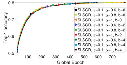
Refer to caption
(a) Top-1 accuracy on testing set
Refer to caption
(b) Cross entropy on training set
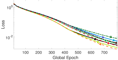
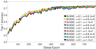
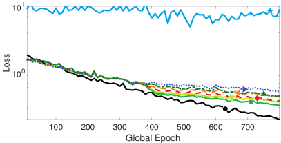
Figure 1: Convergence on training data with balanced partition, without attack. Each epoch is a full pass of the local training data. Legend “SLSGD, γ=0.1,α=0.8,b=2formulae-sequence𝛾0.1formulae-sequence𝛼0.8𝑏2\gamma=0.1,\alpha=0.8,b=2” means that SLSGD takes the learning rate 0.10.10.1 and 𝚃𝚛𝚖𝚎𝚊𝚗2subscript𝚃𝚛𝚖𝚎𝚊𝚗2{\tt Trmean}_{2} for aggregation, and the initial α=1𝛼1\alpha=1 decays by the factor of 0.80.80.8 at the 400400400th epoch. SLSGD with α=1𝛼1\alpha=1 and b=0𝑏0b=0 is the baseline FedAvg. Note that we fix the random seeds. Thus, before α𝛼\alpha decays at the 400400400th epoch, results with the same γ𝛾\gamma and b𝑏b are the same.
Refer to caption
(a) Top-1 accuracy on testing set
Refer to caption
(b) Cross entropy on training set
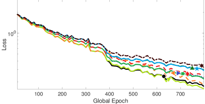
Figure 2: Convergence on training data with unbalanced partition, without attack. Each epoch is a full pass of the local training data. Legend “SLSGD, γ=0.1,α=0.8,b=2formulae-sequence𝛾0.1formulae-sequence𝛼0.8𝑏2\gamma=0.1,\alpha=0.8,b=2” means that SLSGD takes the learning rate 0.10.10.1 and 𝚃𝚛𝚖𝚎𝚊𝚗2subscript𝚃𝚛𝚖𝚎𝚊𝚗2{\tt Trmean}_{2} for aggregation, and the initial α=1𝛼1\alpha=1 decays by the factor of 0.80.80.8 at the 400400400th epoch. SLSGD with α=1𝛼1\alpha=1 and b=0𝑏0b=0 is the baseline FedAvg. Note that we fix the random seeds. Thus, before α𝛼\alpha decays at the 400400400th epoch, results with the same γ𝛾\gamma and b𝑏b are the same.
Refer to caption
(a) Top-1 accuracy on testing set, q=2𝑞2q=2
Refer to caption
(b) Cross entropy on training set, q=2𝑞2q=2
Refer to caption
(c) Top-1 accuracy on testing set, q=4𝑞4q=4
Refer to caption
(d) Cross entropy on training set, q=4𝑞4q=4
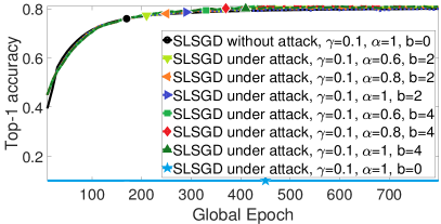
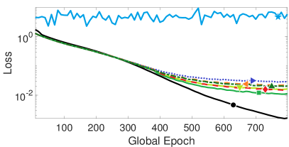
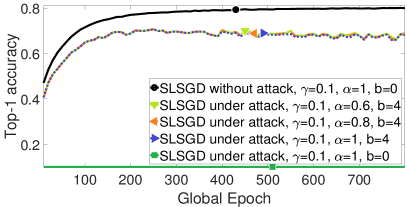
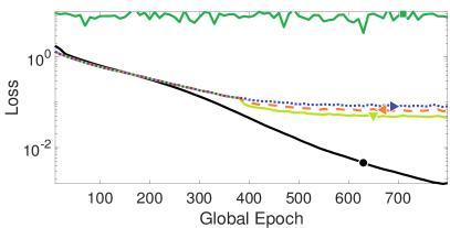
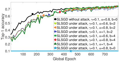
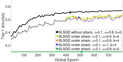
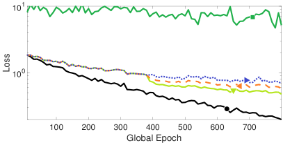
Figure 3: Convergence on training data with balanced partition, with “label-flipping” attack. In each epoch, we guarantee that q{2,4}𝑞24q\in\{2,4\} of the k=10𝑘10k=10 selected workers are poisoned. Each epoch is a full pass of the local training data. Legend “SLSGD, γ=0.1,α=0.8,b=2formulae-sequence𝛾0.1formulae-sequence𝛼0.8𝑏2\gamma=0.1,\alpha=0.8,b=2” means that SLSGD takes the learning rate 0.10.10.1 and 𝚃𝚛𝚖𝚎𝚊𝚗2subscript𝚃𝚛𝚖𝚎𝚊𝚗2{\tt Trmean}_{2} for aggregation, and the initial α=1𝛼1\alpha=1 decays by the factor of 0.80.80.8 at the 400400400th epoch. SLSGD with α=1𝛼1\alpha=1 and b=0𝑏0b=0 is the baseline FedAvg. Note that we fix the random seeds. Thus, before α𝛼\alpha decays at the 400400400th epoch, results with the same γ𝛾\gamma and b𝑏b are the same.
Refer to caption
(a) Top-1 accuracy on testing set, q=2𝑞2q=2
Refer to caption
(b) Cross entropy on training set, q=2𝑞2q=2
Refer to caption
(c) Top-1 accuracy on testing set, q=4𝑞4q=4
Refer to caption
(d) Cross entropy on training set, q=4𝑞4q=4
Figure 4: Convergence on training data with unbalanced partition, with “label-flipping” attack. In each epoch, we guarantee that q𝑞q of the k=10𝑘10k=10 selected workers are poisoned. Each epoch is a full pass of the local training data. Legend “SLSGD, γ=0.1,α=0.8,b=2formulae-sequence𝛾0.1formulae-sequence𝛼0.8𝑏2\gamma=0.1,\alpha=0.8,b=2” means that SLSGD takes the learning rate 0.10.10.1 and 𝚃𝚛𝚖𝚎𝚊𝚗2subscript𝚃𝚛𝚖𝚎𝚊𝚗2{\tt Trmean}_{2} for aggregation, and the initial α=1𝛼1\alpha=1 decays by the factor of 0.80.80.8 at the 400400400th epoch. SLSGD with α=1𝛼1\alpha=1 and b=0𝑏0b=0 is the baseline FedAvg. Note that we fix the random seeds. Thus, before α𝛼\alpha decays at the 400400400th epoch, results with the same γ𝛾\gamma and b𝑏b are the same.

6.2 SLSGD without Attack

We first test the performance of SLSGD on the training data with balanced partition, without data poisoning. The result is shown in Fig. 1. When there are no poisoned workers, using trimmed mean results in extra variance. Although larger b𝑏b and smaller α𝛼\alpha makes the convergence slower, the gap is tiny. In general, SLSGD is insensitive to hyperparameters.

Then, we test the performance with unbalanced partition, without data poisoning. The result is shown in Fig. 2. Note that the convergence with unbalanced partition is generally slower compared to balanced partition due to the larger variance. Using appropriate α𝛼\alpha (α=0.8𝛼0.8\alpha=0.8) can mitigate such extra variance.

6.3 SLSGD under Data Poisoning Attack

To test the tolerance to poisoned workers, we simulate data poisoning which “flips” the labels of the local training data. The poisoned data have “flipped” labels, i.e., each label{0,,9}𝑙𝑎𝑏𝑒𝑙09label\in\{0,\ldots,9\} in the local training data will be replaced by (9label)9𝑙𝑎𝑏𝑒𝑙(9-label). The experiment is set up so that in each epoch, in all the k=10𝑘10k=10 randomly selected workers, q𝑞q workers are compromised and subjected to data poisoning. The results are shown in Fig. 3 and Fig. 4. We use FedAvg/SLSGD without data poisoning (Option I) as the ideal benchmark. As expected, SLSGD without trimmed mean can not tolerate data poisoning, which causes catastrophic failure. SLSGD with Option II tolerates the poisoned worker, though converges slower compared to SLSGD without data poisoning. Furthermore, larger b𝑏b and smaller α𝛼\alpha improves the robustness and stabilizes the convergence.

Note that taking q=4𝑞4q=4 in every epoch pushes to the limit of SLSGD since the algorithm requires 2q<k2𝑞𝑘2q<k. In practice, if there are totally q=4𝑞4q=4 poisoned workers in the entire n=100𝑛100n=100 workers, there is no guarantee that the poisoned workers will always be activated in each epoch. Poisoning 40% of the sampled data in each epoch incurs huge noise, while SLSGD can still prevent the global model from divergence.

In Fig. 5, we show how α𝛼\alpha and b𝑏b affect the convergence when data poisoning and unbalanced partition cause extra error and variance. In such scenario, larger b𝑏b and smaller α𝛼\alpha makes SLSGD more robust and converge faster.

Refer to caption
Figure 5: Number of global epochs to reach training loss value 0.50.50.5, with unbalanced partition and q=2𝑞2q=2 poisoned workers. γ=0.1𝛾0.1\gamma=0.1. α𝛼\alpha and b𝑏b varies. “α𝛼\alpha” on the x-axis is the initial value of α𝛼\alpha, which does not decay during training.
Refer to caption
Figure 6: Number of global epochs to reach training loss value 0.0030.0030.003, with balanced partition, without poisoned workers. γ=0.1𝛾0.1\gamma=0.1. α𝛼\alpha and number of local iterations varies. “pass=3” means each epoch is 3 full passes of the local datasets on the selected workers. “α𝛼\alpha” on the x-axis is the initial value of α𝛼\alpha, which does not decay during training.

6.4 Acceleration by Local Updates

According to our theoretical analysis, more local updates in each epoch accelerate the convergence. We test this theory in Fig. 6 with balanced partition, without data poisoning. In the legend, “pass=3” means each epoch is 3 full passes of the local datasets (H=3×500/50=30𝐻35005030H=3\times 500/50=30 local iterations) on the selected workers. We show that with more local iterations, SLSGD converges faster.

6.5 Discussion

The hyperparameters of SLSGD affects the convergence differently in different scenarios:

  • Balanced partition, no attacks. In this case, the overall variance is relatively small. Thus, it is not necessary to use smaller α𝛼\alpha to mitigate the variance. The extra variance caused by trimmed mean slows down the convergence. Since the variance does not dominate, smaller α𝛼\alpha and larger b𝑏b potentially slow down the convergence, but the gap is tiny.

  • Unbalanced partition, no attacks. In this case, the overall variance is larger than the balanced case. Note that not only the size of local datasets, but also the label distribution are unbalanced among the devices. Some partitions only contains one label, which enlarges the accumulative error caused by infrequent synchronization and overfitting the local training data. Thus, using appropriate α𝛼\alpha can mitigate the variance. However, it is not necessary to use the trimmed mean, since the variance caused by unbalanced partition is not too bad compared to data poisoning.

  • Balanced partition, under attacks. In this case, the error caused by poisoned workers dominates. We must use trimmed mean to prevent divergence. Larger b𝑏b improves the robustness and convergence. Furthermore, using smaller α𝛼\alpha also mitigates the error and improves the convergence.

  • Unbalanced partition, under attacks. In this case, the error caused by poisoned workers still dominates. In general, the usage of hyperparameters is similar to the case of balanced partition under attacks. However, the unbalanced partition makes it more difficult to distinguish poisoned workers from normal workers. As a result, the convergence gets much slower. Smaller α𝛼\alpha obtain more improvement and better stabilization.

In general, there is a trade-off between convergence rate and variance/error reduction. In the ideal case, if the variance is very small, SLSGD with α=1𝛼1\alpha=1 and b=0𝑏0b=0, i.e., FedAvg, has fastest convergence. Using other hyperparameters slightly slows down the convergence, but the gap is tiny. When variance gets larger, users can try smaller α𝛼\alpha. When the variance/error gets catastrophically large, the users can use the trimmed mean to prevent divergence.

7 Conclusion

We propose a novel distributed optimization algorithm on non-IID training data, which has limited communication and tolerates poisoned workers. The algorithm has provable convergence. Our empirical results show good performance in practice. In future work, we are going to analyze our algorithm on other threat models, such as hardware or software failures.

References

  • [1] Anguita, D., Ghio, A., Oneto, L., Parra, X., Reyes-Ortiz, J.L.: A public domain dataset for human activity recognition using smartphones. In: ESANN (2013)
  • [2] Bae, H., Jang, J., Jung, D., Jang, H., Ha, H., Yoon, S.: Security and privacy issues in deep learning. arXiv preprint arXiv:1807.11655 (2018)
  • [3] Bagdasaryan, E., Veit, A., Hua, Y., Estrin, D., Shmatikov, V.: How to backdoor federated learning. arXiv preprint arXiv:1807.00459 (2018)
  • [4] Bhagoji, A.N., Chakraborty, S., Mittal, P., Calo, S.: Analyzing federated learning through an adversarial lens. arXiv preprint arXiv:1811.12470 (2018)
  • [5] Cao, Y., Hou, P., Brown, D., Wang, J., Chen, S.: Distributed analytics and edge intelligence: Pervasive health monitoring at the era of fog computing. In: Proceedings of the 2015 Workshop on Mobile Big Data. pp. 43–48. ACM (2015)
  • [6] Chen, T., Li, M., Li, Y., Lin, M., Wang, N., Wang, M., Xiao, T., Xu, B., Zhang, C., Zhang, Z.: Mxnet: A flexible and efficient machine learning library for heterogeneous distributed systems. arXiv preprint arXiv:1512.01274 (2015)
  • [7] Chen, Y., Su, L., Xu, J.: Distributed statistical machine learning in adversarial settings: Byzantine gradient descent. ACM SIGMETRICS Performance Evaluation Review 46(1), 96–96 (2019)
  • [8] EU: European Union’s General Data Protection Regulation (GDPR) (2018), https://eugdpr.org/, Last visited: Nov. 2018
  • [9] Fung, C., Yoon, C.J., Beschastnikh, I.: Mitigating sybils in federated learning poisoning. arXiv preprint arXiv:1808.04866 (2018)
  • [10] Garcia Lopez, P., Montresor, A., Epema, D., Datta, A., Higashino, T., Iamnitchi, A., Barcellos, M., Felber, P., Riviere, E.: Edge-centric computing: Vision and challenges. ACM SIGCOMM Computer Communication Review 45(5), 37–42 (2015)
  • [11] gluon-nlp.mxnet.io: LSTM-based Language Models (2019), https://gluon-nlp.mxnet.io/master/examples/language_model/language_model.html, Last visited: Mar. 2019
  • [12] HealthInsurance.org, S.A.: Health insurance portability and accountability act of 1996. Public law 104,  191 (1996)
  • [13] Ho, Q., Cipar, J., Cui, H., Lee, S., Kim, J.K., Gibbons, P.B., Gibson, G.A., Ganger, G., Xing, E.P.: More effective distributed ml via a stale synchronous parallel parameter server. In: Advances in neural information processing systems. pp. 1223–1231 (2013)
  • [14] Hong, K., Lillethun, D., Ramachandran, U., Ottenwälder, B., Koldehofe, B.: Mobile fog: A programming model for large-scale applications on the internet of things. In: Proceedings of the second ACM SIGCOMM workshop on Mobile cloud computing. pp. 15–20. ACM (2013)
  • [15] Howard, A.G., Zhu, M., Chen, B., Kalenichenko, D., Wang, W., Weyand, T., Andreetto, M., Adam, H.: Mobilenets: Efficient convolutional neural networks for mobile vision applications. arXiv preprint arXiv:1704.04861 (2017)
  • [16] Konečnỳ, J., McMahan, B., Ramage, D.: Federated optimization: Distributed optimization beyond the datacenter. arXiv preprint arXiv:1511.03575 (2015)
  • [17] Konečnỳ, J., McMahan, H.B., Yu, F.X., Richtárik, P., Suresh, A.T., Bacon, D.: Federated learning: Strategies for improving communication efficiency. arXiv preprint arXiv:1610.05492 (2016)
  • [18] Krizhevsky, A., Hinton, G.: Learning multiple layers of features from tiny images. Tech. rep., Citeseer (2009)
  • [19] Li, M., Andersen, D.G., Park, J.W., Smola, A.J., Ahmed, A., Josifovski, V., Long, J., Shekita, E.J., Su, B.Y.: Scaling distributed machine learning with the parameter server. In: OSDI. vol. 14, pp. 583–598 (2014)
  • [20] Li, M., Andersen, D.G., Smola, A.J., Yu, K.: Communication efficient distributed machine learning with the parameter server. In: Advances in Neural Information Processing Systems. pp. 19–27 (2014)
  • [21] Mahdavinejad, M.S., Rezvan, M., Barekatain, M., Adibi, P., Barnaghi, P., Sheth, A.P.: Machine learning for internet of things data analysis: A survey. Digital Communications and Networks 4(3), 161–175 (2018)
  • [22] McMahan, H.B., Moore, E., Ramage, D., Hampson, S., et al.: Communication-efficient learning of deep networks from decentralized data. arXiv preprint arXiv:1602.05629 (2016)
  • [23] Merity, S., Xiong, C., Bradbury, J., Socher, R.: Pointer sentinel mixture models. arXiv preprint arXiv:1609.07843 (2016)
  • [24] Pantelopoulos, A., Bourbakis, N.G.: A survey on wearable sensor-based systems for health monitoring and prognosis. IEEE Transactions on Systems, Man, and Cybernetics, Part C (Applications and Reviews) 40(1), 1–12 (2010)
  • [25] source.android.com: Key and ID Attestation (2019), https://source.android.com/security/keystore/attestation, Last visited: Mar. 2019
  • [26] Stich, S.U.: Local sgd converges fast and communicates little. arXiv preprint arXiv:1805.09767 (2018)
  • [27] Xie, C., Koyejo, O., Gupta, I.: Phocas: dimensional byzantine-resilient stochastic gradient descent. arXiv preprint arXiv:1805.09682 (2018)
  • [28] Yin, D., Chen, Y., Ramchandran, K., Bartlett, P.: Byzantine-robust distributed learning: Towards optimal statistical rates. arXiv preprint arXiv:1803.01498 (2018)
  • [29] Yu, H., Yang, S., Zhu, S.: Parallel restarted sgd for non-convex optimization with faster convergence and less communication. arXiv preprint arXiv:1807.06629 (2018)
  • [30] Zeydan, E., Bastug, E., Bennis, M., Kader, M.A., Karatepe, I.A., Er, A.S., Debbah, M.: Big data caching for networking: Moving from cloud to edge. IEEE Communications Magazine 54(9), 36–42 (2016)

Appendix

8 Additional Experiments

8.1 CNN on CIFAR-10

We conduct experiments on the benchmark CIFAR-10 image classification dataset [18], which is composed of 50k images for training and 10k images for testing. Each image is resized and cropped to the shape of (24,24,3)24243(24,24,3). We use convolutional neural network (CNN) with 4 convolutional layers followed by 1 fully connected layer. We use a simple network architecture, so that it can be easily handled by edge devices. The detailed network architecture can be found in our submitted source code (will also be released upon publication). The experiments are conducted on CPU devices. We implement SLSGD using the MXNET [6] framework. The results are shown in Fig. 7, 8, 9, and 10.

Refer to caption
(a) Top-1 accuracy on testing set, γ=0.1𝛾0.1\gamma=0.1
Refer to caption
(b) Cross entropy on training set, γ=0.1𝛾0.1\gamma=0.1
Refer to caption
(c) Top-1 accuracy on testing set, γ=0.05𝛾0.05\gamma=0.05
Refer to caption
(d) Cross entropy on training set, γ=0.05𝛾0.05\gamma=0.05
Figure 7: CNN experiment on CIFAR-10. Convergence on training data with unbalanced partition, without attack. Each epoch is a full pass of the local training data. Legend “SLSGD, γ=0.1,α=0.8,b=2formulae-sequence𝛾0.1formulae-sequence𝛼0.8𝑏2\gamma=0.1,\alpha=0.8,b=2” means that SLSGD takes the learning rate 0.10.10.1 and 𝚃𝚛𝚖𝚎𝚊𝚗2subscript𝚃𝚛𝚖𝚎𝚊𝚗2{\tt Trmean}_{2} for aggregation, and the initial α=1𝛼1\alpha=1 decays by the factor of 0.80.80.8 at the 400400400th epoch. Note that SLSGD with α=1𝛼1\alpha=1 and b=0𝑏0b=0 is the baseline FedAvg. Note that we fix the random seeds. Thus, before α𝛼\alpha decays at the 400400400th epoch, results with the same γ𝛾\gamma and b𝑏b are the same.
Refer to caption
(a) Top-1 accuracy on testing set, γ=0.1𝛾0.1\gamma=0.1
Refer to caption
(b) Cross entropy on training set, γ=0.1𝛾0.1\gamma=0.1
Refer to caption
(c) Top-1 accuracy on testing set, γ=0.05𝛾0.05\gamma=0.05
Refer to caption
(d) Cross entropy on training set, γ=0.05𝛾0.05\gamma=0.05
Figure 8: CNN experiment on CIFAR-10. Convergence on training data with unbalanced partition, without attack. Each epoch is a full pass of the local training data. Legend “SLSGD, γ=0.1,α=0.8,b=2formulae-sequence𝛾0.1formulae-sequence𝛼0.8𝑏2\gamma=0.1,\alpha=0.8,b=2” means that SLSGD takes the learning rate 0.10.10.1 and 𝚃𝚛𝚖𝚎𝚊𝚗2subscript𝚃𝚛𝚖𝚎𝚊𝚗2{\tt Trmean}_{2} for aggregation, and the initial α=1𝛼1\alpha=1 decays by the factor of 0.80.80.8 at the 400400400th epoch. Note that SLSGD with α=1𝛼1\alpha=1 and b=0𝑏0b=0 is the baseline FedAvg. Note that we fix the random seeds. Thus, before α𝛼\alpha decays at the 400400400th epoch, results with the same γ𝛾\gamma and b𝑏b are the same.
Refer to caption
(a) Top-1 accuracy on testing set, q=2𝑞2q=2
Refer to caption
(b) Cross entropy on training set, q=2𝑞2q=2
Refer to caption
(c) Top-1 accuracy on testing set, q=4𝑞4q=4
Refer to caption
(d) Cross entropy on training set, q=4𝑞4q=4
Figure 9: CNN experiment on CIFAR-10. Convergence on training data with balanced partition, with “label-flipping” attack. In each epoch, we guarantee that q{2,4}𝑞24q\in\{2,4\} of the k=10𝑘10k=10 selected workers are poisoned. Each epoch is a full pass of the local training data. Legend “SLSGD, γ=0.1,α=0.8,b=2formulae-sequence𝛾0.1formulae-sequence𝛼0.8𝑏2\gamma=0.1,\alpha=0.8,b=2” means that SLSGD takes the learning rate 0.10.10.1 and 𝚃𝚛𝚖𝚎𝚊𝚗2subscript𝚃𝚛𝚖𝚎𝚊𝚗2{\tt Trmean}_{2} for aggregation, and the initial α=1𝛼1\alpha=1 decays by the factor of 0.80.80.8 at the 400400400th epoch. Note that SLSGD with α=1𝛼1\alpha=1 and b=0𝑏0b=0 is the baseline FedAvg. Note that we fix the random seeds. Thus, before α𝛼\alpha decays at the 400400400th epoch, results with the same γ𝛾\gamma and b𝑏b are the same.
Refer to caption
(a) Top-1 accuracy on testing set, q=2𝑞2q=2
Refer to caption
(b) Cross entropy on training set, q=2𝑞2q=2
Refer to caption
(c) Top-1 accuracy on testing set, q=4𝑞4q=4
Refer to caption
(d) Cross entropy on training set, q=4𝑞4q=4
Figure 10: CNN experiment on CIFAR-10. Convergence on training data with unbalanced partition, with “label-flipping” attack. In each epoch, we guarantee that q𝑞q of the k=10𝑘10k=10 selected workers are poisoned. Each epoch is a full pass of the local training data. Legend “SLSGD, γ=0.1,α=0.8,b=2formulae-sequence𝛾0.1formulae-sequence𝛼0.8𝑏2\gamma=0.1,\alpha=0.8,b=2” means that SLSGD takes the learning rate 0.10.10.1 and 𝚃𝚛𝚖𝚎𝚊𝚗2subscript𝚃𝚛𝚖𝚎𝚊𝚗2{\tt Trmean}_{2} for aggregation, and the initial α=1𝛼1\alpha=1 decays by the factor of 0.80.80.8 at the 400400400th epoch. Note that SLSGD with α=1𝛼1\alpha=1 and b=0𝑏0b=0 is the baseline FedAvg. Note that we fix the random seeds. Thus, before α𝛼\alpha decays at the 400400400th epoch, results with the same γ𝛾\gamma and b𝑏b are the same.

8.2 LSTM on WikiText-2

We conduct experiments on WikiText-2 dataset [23]. We use LSTM-based language model. The model architecture was taken from the MXNET and Gluon-NLP tutorial [11]. The detailed network architecture can be found in our submitted source code (will also be released upon publication). The experiments are conducted on CPU devices. We implement SLSGD using the MXNET [6] framework.

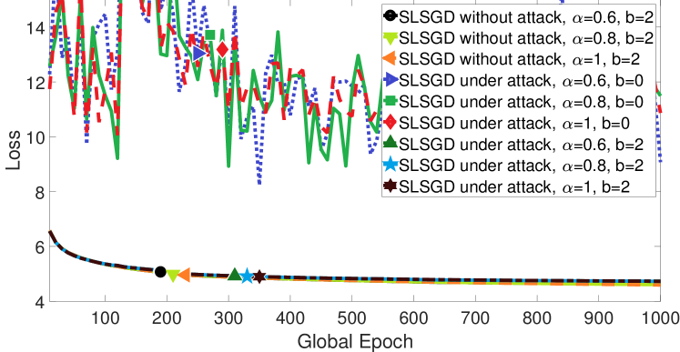
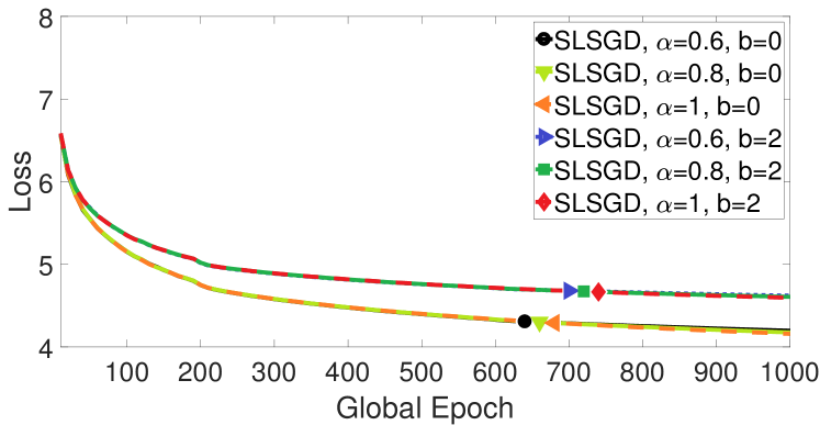
Similar to the CNN experiments, the dataset is partitioned onto 100 devices. In each global epoch, 10 devices are activated for training. The results are shown in Fig. 11, 12, and 13. For the poisoned workers, the labels of the local training data are randomly permuted.

In general, we get similar results as CNN on CIFAR-10.
Refer to caption
Figure 11: LSTM experiment on WikiText-2. Convergence on training data with balanced partition, without attack. Each epoch is a full pass of the local training data. We take learning rate γ=20𝛾20\gamma=20. Legend “SLSGD, α=0.8,b=2formulae-sequence𝛼0.8𝑏2\alpha=0.8,b=2” means that SLSGD takes 𝚃𝚛𝚖𝚎𝚊𝚗2subscript𝚃𝚛𝚖𝚎𝚊𝚗2{\tt Trmean}_{2} for aggregation, and the initial α=1𝛼1\alpha=1 decays by the factor of 0.80.80.8 at the 600600600th epoch. Note that SLSGD with α=1𝛼1\alpha=1 and b=0𝑏0b=0 is the baseline FedAvg. Note that we fix the random seeds. Thus, before α𝛼\alpha decays at the 600600600th epoch, results with the same γ𝛾\gamma and b𝑏b are the same.
Refer to caption
Figure 12: LSTM experiment on WikiText-2. Convergence on training data with balanced partition, under attack. In each epoch, we guarantee that q=2𝑞2q=2 of the k=10𝑘10k=10 selected workers are training on poisoned data. Each epoch is a full pass of the local training data. We take learning rate γ=20𝛾20\gamma=20. Legend “SLSGD, α=0.8,b=2formulae-sequence𝛼0.8𝑏2\alpha=0.8,b=2” means that SLSGD takes 𝚃𝚛𝚖𝚎𝚊𝚗2subscript𝚃𝚛𝚖𝚎𝚊𝚗2{\tt Trmean}_{2} for aggregation, and the initial α=1𝛼1\alpha=1 decays by the factor of 0.80.80.8 at the 600600600th epoch. Note that SLSGD with α=1𝛼1\alpha=1 and b=0𝑏0b=0 is the baseline FedAvg. Note that we fix the random seeds. Thus, before α𝛼\alpha decays at the 600600600th epoch, results with the same γ𝛾\gamma and b𝑏b are the same.
Refer to caption
Figure 13: (Zoomed) LSTM experiment on WikiText-2. Convergence on training data with balanced partition, under attack. In each epoch, we guarantee that q=2𝑞2q=2 of the k=10𝑘10k=10 selected workers are training on poisoned data. Each epoch is a full pass of the local training data. We take learning rate γ=20𝛾20\gamma=20. Legend “SLSGD, α=0.8,b=2formulae-sequence𝛼0.8𝑏2\alpha=0.8,b=2” means that SLSGD takes 𝚃𝚛𝚖𝚎𝚊𝚗2subscript𝚃𝚛𝚖𝚎𝚊𝚗2{\tt Trmean}_{2} for aggregation, and the initial α=1𝛼1\alpha=1 decays by the factor of 0.80.80.8 at the 600600600th epoch. Note that SLSGD with α=1𝛼1\alpha=1 and b=0𝑏0b=0 is the baseline FedAvg. Note that we fix the random seeds. Thus, before α𝛼\alpha decays at the 600600600th epoch, results with the same γ𝛾\gamma and b𝑏b are the same.

9 Proofs

Theorem 9.1

We take γmin(1L,2)𝛾1𝐿2\gamma\leq\min\left(\frac{1}{L},2\right). After T𝑇T epochs, Algorithm 1 with Option I converges to a global optimum:

𝔼[F(xT)F(x)](1α+α(1γ2)Hmin)T[F(x0)F(x)]𝔼delimited-[]𝐹subscript𝑥𝑇𝐹subscript𝑥superscript1𝛼𝛼superscript1𝛾2subscript𝐻𝑚𝑖𝑛𝑇delimited-[]𝐹subscript𝑥0𝐹subscript𝑥\displaystyle{\mathbb{E}}\left[F(x_{T})-F(x_{*})\right]\leq\left(1-\alpha+\alpha(1-\frac{\gamma}{2})^{H_{min}}\right)^{T}\left[F(x_{0})-F(x_{*})\right]
+[1(1α+α(1γ2)Hmin)T]𝒪(V1+(1+1k1n)V2),delimited-[]1superscript1𝛼𝛼superscript1𝛾2subscript𝐻𝑚𝑖𝑛𝑇𝒪subscript𝑉111𝑘1𝑛subscript𝑉2\displaystyle\quad+\left[1-\left(1-\alpha+\alpha(1-\frac{\gamma}{2})^{H_{min}}\right)^{T}\right]\mathcal{O}\left(V_{1}+\left(1+\frac{1}{k}-\frac{1}{n}\right)V_{2}\right),

where V2=maxt{0,T1},h{0,Hti1},i[n]xt,hix2subscript𝑉2subscriptformulae-sequence𝑡0𝑇1formulae-sequence0subscriptsuperscript𝐻𝑖𝑡1𝑖delimited-[]𝑛superscriptnormsuperscriptsubscript𝑥𝑡𝑖subscript𝑥2V_{2}=\max_{t\in\{0,T-1\},h\in\{0,H^{i}_{t}-1\},i\in[n]}\|x_{t,h}^{i}-x_{*}\|^{2}.

Proof

For convenience, we ignore the random sample z𝒟isimilar-to𝑧superscript𝒟𝑖z\sim\mathcal{D}^{i} in our notations. Thus, fi(xt,hi)superscript𝑓𝑖superscriptsubscript𝑥𝑡𝑖f^{i}(x_{t,h}^{i}) represents f(xt,hi;zt,hi)𝑓superscriptsubscript𝑥𝑡𝑖superscriptsubscript𝑧𝑡𝑖f(x_{t,h}^{i};z_{t,h}^{i}), where zt,hi𝒟isimilar-tosuperscriptsubscript𝑧𝑡𝑖superscript𝒟𝑖z_{t,h}^{i}\sim\mathcal{D}^{i}. Furthermore, we define Fi(x)=𝔼z𝒟if(x;z)superscript𝐹𝑖𝑥subscript𝔼similar-to𝑧superscript𝒟𝑖𝑓𝑥𝑧F^{i}(x)={\mathbb{E}}_{z\sim\mathcal{D}^{i}}f(x;z).

Thus, Line 10 in Algorithm 1 can be rewritten into

xt,hi=xt,h1iγfti(xt,h1i).superscriptsubscript𝑥𝑡𝑖superscriptsubscript𝑥𝑡1𝑖𝛾subscriptsuperscript𝑓𝑖𝑡superscriptsubscript𝑥𝑡1𝑖\displaystyle x_{t,h}^{i}=x_{t,h-1}^{i}-\gamma\nabla f^{i}_{t}(x_{t,h-1}^{i}).

Using L𝐿L-smoothness of F(x)𝐹𝑥F(x), we have

F(xt,hi)𝐹superscriptsubscript𝑥𝑡𝑖\displaystyle F(x_{t,h}^{i})
F(xt,h1i)γF(xt,h1i,fi(xt,h1i)+Lγ22fi(xt,h1i)2\displaystyle\leq F(x_{t,h-1}^{i})-\gamma\left\langle\nabla F(x_{t,h-1}^{i},\nabla f^{i}(x_{t,h-1}^{i})\right\rangle+\frac{L\gamma^{2}}{2}\left\|\nabla f^{i}(x_{t,h-1}^{i})\right\|^{2}
F(xt,h1i)γF(xt,h1i,fi(xt,h1i)+γ2fi(xt,h1i)2\displaystyle\leq F(x_{t,h-1}^{i})-\gamma\left\langle\nabla F(x_{t,h-1}^{i},\nabla f^{i}(x_{t,h-1}^{i})\right\rangle+\frac{\gamma}{2}\left\|\nabla f^{i}(x_{t,h-1}^{i})\right\|^{2}
F(xt,h1i)γ2F(xt,h1i)2+γ2F(xt,h1i)fi(xt,h1i)2.absent𝐹superscriptsubscript𝑥𝑡1𝑖𝛾2superscriptnorm𝐹superscriptsubscript𝑥𝑡1𝑖2𝛾2superscriptnorm𝐹superscriptsubscript𝑥𝑡1𝑖superscript𝑓𝑖superscriptsubscript𝑥𝑡1𝑖2\displaystyle\leq F(x_{t,h-1}^{i})-\frac{\gamma}{2}\left\|\nabla F(x_{t,h-1}^{i})\right\|^{2}+\frac{\gamma}{2}\left\|\nabla F(x_{t,h-1}^{i})-f^{i}(x_{t,h-1}^{i})\right\|^{2}.

It is easy to check that ρ0𝜌0\exists\rho\geq 0, G(x)=F(x)+ρ2xx2subscript𝐺𝑥𝐹𝑥𝜌2superscriptnorm𝑥subscript𝑥2G_{*}(x)=F(x)+\frac{\rho}{2}\|x-x_{*}\|^{2} is (ρ+μ)𝜌𝜇(\rho+\mu)-strongly convex, where ρ+μ1𝜌𝜇1\rho+\mu\geq 1. Thus, we have

F(x)F(x)G(x)G(x)G(x)22(ρ+μ)F(x)2+ρ2xx2ρ+μ.𝐹𝑥𝐹subscript𝑥subscript𝐺𝑥subscript𝐺subscript𝑥superscriptnormsubscript𝐺𝑥22𝜌𝜇superscriptnorm𝐹𝑥2superscript𝜌2superscriptnorm𝑥subscript𝑥2𝜌𝜇\displaystyle F(x)-F(x_{*})\leq G_{*}(x)-G_{*}(x_{*})\leq\frac{\|\nabla G_{*}(x)\|^{2}}{2(\rho+\mu)}\leq\frac{\|\nabla F(x)\|^{2}+\rho^{2}\|x-x_{*}\|^{2}}{\rho+\mu}.

Taking expectation on both sides, conditional on xt,h1isuperscriptsubscript𝑥𝑡1𝑖x_{t,h-1}^{i}, we have

𝔼[F(xt,hi)F(x)]𝔼delimited-[]𝐹superscriptsubscript𝑥𝑡𝑖𝐹subscript𝑥\displaystyle{\mathbb{E}}\left[F(x_{t,h}^{i})-F(x_{*})\right]
F(xt,h1i)F(x)γ2F(xt,h1i)2+γV1absent𝐹superscriptsubscript𝑥𝑡1𝑖𝐹subscript𝑥𝛾2superscriptnorm𝐹superscriptsubscript𝑥𝑡1𝑖2𝛾subscript𝑉1\displaystyle\leq F(x_{t,h-1}^{i})-F(x_{*})-\frac{\gamma}{2}\left\|\nabla F(x_{t,h-1}^{i})\right\|^{2}+\gamma V_{1}
F(xt,h1i)F(x)γ2(ρ+μ)[F(xt,h1i)F(x)]+γρ22xt,h1ix2+γV1absent𝐹superscriptsubscript𝑥𝑡1𝑖𝐹subscript𝑥𝛾2𝜌𝜇delimited-[]𝐹superscriptsubscript𝑥𝑡1𝑖𝐹subscript𝑥𝛾superscript𝜌22superscriptnormsuperscriptsubscript𝑥𝑡1𝑖subscript𝑥2𝛾subscript𝑉1\displaystyle\leq F(x_{t,h-1}^{i})-F(x_{*})-\frac{\gamma}{2}(\rho+\mu)\left[F(x_{t,h-1}^{i})-F(x_{*})\right]+\frac{\gamma\rho^{2}}{2}\|x_{t,h-1}^{i}-x_{*}\|^{2}+\gamma V_{1}
(1γ2)[F(xt,h1i)F(x)]+γ𝒪(V1+V2).absent1𝛾2delimited-[]𝐹superscriptsubscript𝑥𝑡1𝑖𝐹subscript𝑥𝛾𝒪subscript𝑉1subscript𝑉2\displaystyle\leq(1-\frac{\gamma}{2})\left[F(x_{t,h-1}^{i})-F(x_{*})\right]+\gamma\mathcal{O}(V_{1}+V_{2}).

By telescoping and taking total expectation, we have

𝔼[F(xt,Htii)F(x)]𝔼delimited-[]𝐹superscriptsubscript𝑥𝑡subscriptsuperscript𝐻𝑖𝑡𝑖𝐹subscript𝑥\displaystyle{\mathbb{E}}\left[F(x_{t,H^{i}_{t}}^{i})-F(x_{*})\right]
(1γ2)Hti[F(xt,0i)F(x)]+1(1γ2)Hti1(1γ2)γ𝒪(V1+V2)absentsuperscript1𝛾2subscriptsuperscript𝐻𝑖𝑡delimited-[]𝐹superscriptsubscript𝑥𝑡0𝑖𝐹subscript𝑥1superscript1𝛾2subscriptsuperscript𝐻𝑖𝑡11𝛾2𝛾𝒪subscript𝑉1subscript𝑉2\displaystyle\leq(1-\frac{\gamma}{2})^{H^{i}_{t}}\left[F(x_{t,0}^{i})-F(x_{*})\right]+\frac{1-(1-\frac{\gamma}{2})^{H^{i}_{t}}}{1-(1-\frac{\gamma}{2})}\gamma\mathcal{O}(V_{1}+V_{2})
(1γ2)Hmin[F(xt,0i)F(x)]+𝒪(V1+V2).absentsuperscript1𝛾2subscript𝐻𝑚𝑖𝑛delimited-[]𝐹superscriptsubscript𝑥𝑡0𝑖𝐹subscript𝑥𝒪subscript𝑉1subscript𝑉2\displaystyle\leq(1-\frac{\gamma}{2})^{H_{min}}\left[F(x_{t,0}^{i})-F(x_{*})\right]+\mathcal{O}(V_{1}+V_{2}).

St[n]subscript𝑆𝑡delimited-[]𝑛S_{t}\subseteq[n] is a subset of devices randomly sampled from all the n𝑛n devices without placement. Thus, we have

F(1kiStxt,Htii)𝐹1𝑘subscript𝑖subscript𝑆𝑡superscriptsubscript𝑥𝑡subscriptsuperscript𝐻𝑖𝑡𝑖\displaystyle F\left(\frac{1}{k}\sum_{i\in S_{t}}x_{t,H^{i}_{t}}^{i}\right)
F(1ni[n]xt,Htii)+F(1ni[n]xt,Htii),1kiStxt,Htii1ni[n]xt,Htiiabsent𝐹1𝑛subscript𝑖delimited-[]𝑛superscriptsubscript𝑥𝑡subscriptsuperscript𝐻𝑖𝑡𝑖𝐹1𝑛subscript𝑖delimited-[]𝑛superscriptsubscript𝑥𝑡subscriptsuperscript𝐻𝑖𝑡𝑖1𝑘subscript𝑖subscript𝑆𝑡superscriptsubscript𝑥𝑡subscriptsuperscript𝐻𝑖𝑡𝑖1𝑛subscript𝑖delimited-[]𝑛superscriptsubscript𝑥𝑡subscriptsuperscript𝐻𝑖𝑡𝑖\displaystyle\leq F\left(\frac{1}{n}\sum_{i\in[n]}x_{t,H^{i}_{t}}^{i}\right)+\left\langle\nabla F\left(\frac{1}{n}\sum_{i\in[n]}x_{t,H^{i}_{t}}^{i}\right),\frac{1}{k}\sum_{i\in S_{t}}x_{t,H^{i}_{t}}^{i}-\frac{1}{n}\sum_{i\in[n]}x_{t,H^{i}_{t}}^{i}\right\rangle
+L21kiStxt,Htii1ni[n]xt,Htii2𝐿2superscriptnorm1𝑘subscript𝑖subscript𝑆𝑡superscriptsubscript𝑥𝑡subscriptsuperscript𝐻𝑖𝑡𝑖1𝑛subscript𝑖delimited-[]𝑛superscriptsubscript𝑥𝑡subscriptsuperscript𝐻𝑖𝑡𝑖2\displaystyle\quad+\frac{L}{2}\left\|\frac{1}{k}\sum_{i\in S_{t}}x_{t,H^{i}_{t}}^{i}-\frac{1}{n}\sum_{i\in[n]}x_{t,H^{i}_{t}}^{i}\right\|^{2}
F(1ni[n]xt,Htii)+12F(1ni[n]xt,Htii)2+L+121kiStxt,Htii1ni[n]xt,Htii2absent𝐹1𝑛subscript𝑖delimited-[]𝑛superscriptsubscript𝑥𝑡subscriptsuperscript𝐻𝑖𝑡𝑖12superscriptnorm𝐹1𝑛subscript𝑖delimited-[]𝑛superscriptsubscript𝑥𝑡subscriptsuperscript𝐻𝑖𝑡𝑖2𝐿12superscriptnorm1𝑘subscript𝑖subscript𝑆𝑡superscriptsubscript𝑥𝑡subscriptsuperscript𝐻𝑖𝑡𝑖1𝑛subscript𝑖delimited-[]𝑛superscriptsubscript𝑥𝑡subscriptsuperscript𝐻𝑖𝑡𝑖2\displaystyle\leq F\left(\frac{1}{n}\sum_{i\in[n]}x_{t,H^{i}_{t}}^{i}\right)+\frac{1}{2}\left\|\nabla F\left(\frac{1}{n}\sum_{i\in[n]}x_{t,H^{i}_{t}}^{i}\right)\right\|^{2}+\frac{L+1}{2}\left\|\frac{1}{k}\sum_{i\in S_{t}}x_{t,H^{i}_{t}}^{i}-\frac{1}{n}\sum_{i\in[n]}x_{t,H^{i}_{t}}^{i}\right\|^{2}
F(1ni[n]xt,Htii)+𝒪(V1)+(1k1n)1n1i[n]L+12xt,Htii1nj[n]xt,Htjj2absent𝐹1𝑛subscript𝑖delimited-[]𝑛superscriptsubscript𝑥𝑡subscriptsuperscript𝐻𝑖𝑡𝑖𝒪subscript𝑉11𝑘1𝑛1𝑛1subscript𝑖delimited-[]𝑛𝐿12superscriptnormsuperscriptsubscript𝑥𝑡subscriptsuperscript𝐻𝑖𝑡𝑖1𝑛subscript𝑗delimited-[]𝑛superscriptsubscript𝑥𝑡subscriptsuperscript𝐻𝑗𝑡𝑗2\displaystyle\leq F\left(\frac{1}{n}\sum_{i\in[n]}x_{t,H^{i}_{t}}^{i}\right)+\mathcal{O}(V_{1})+\left(\frac{1}{k}-\frac{1}{n}\right)\frac{1}{n-1}\sum_{i\in[n]}\frac{L+1}{2}\left\|x_{t,H^{i}_{t}}^{i}-\frac{1}{n}\sum_{j\in[n]}x_{t,H^{j}_{t}}^{j}\right\|^{2}
F(1ni[n]xt,Htii)+𝒪(V1)+(1k1n)𝒪(V2).absent𝐹1𝑛subscript𝑖delimited-[]𝑛superscriptsubscript𝑥𝑡subscriptsuperscript𝐻𝑖𝑡𝑖𝒪subscript𝑉11𝑘1𝑛𝒪subscript𝑉2\displaystyle\leq F\left(\frac{1}{n}\sum_{i\in[n]}x_{t,H^{i}_{t}}^{i}\right)+\mathcal{O}(V_{1})+\left(\frac{1}{k}-\frac{1}{n}\right)\mathcal{O}(V_{2}).

On the server, after aggregation, conditional on xt1subscript𝑥𝑡1x_{t-1}, we have

𝔼[F(xt)F(x)]𝔼delimited-[]𝐹subscriptsuperscript𝑥𝑡𝐹subscript𝑥\displaystyle{\mathbb{E}}\left[F(x^{\prime}_{t})-F(x_{*})\right]
𝔼[G(1ni[n]xt,Htii)F(x)]+𝔼[F(1kiStxt,Htii)F(1ni[n]xt,Htii)]absent𝔼delimited-[]subscript𝐺1𝑛subscript𝑖delimited-[]𝑛superscriptsubscript𝑥𝑡subscriptsuperscript𝐻𝑖𝑡𝑖𝐹subscript𝑥𝔼delimited-[]𝐹1𝑘subscript𝑖subscript𝑆𝑡superscriptsubscript𝑥𝑡subscriptsuperscript𝐻𝑖𝑡𝑖𝐹1𝑛subscript𝑖delimited-[]𝑛superscriptsubscript𝑥𝑡subscriptsuperscript𝐻𝑖𝑡𝑖\displaystyle\leq{\mathbb{E}}\left[G_{*}(\frac{1}{n}\sum_{i\in[n]}x_{t,H^{i}_{t}}^{i})-F(x_{*})\right]+{\mathbb{E}}\left[F\left(\frac{1}{k}\sum_{i\in S_{t}}x_{t,H^{i}_{t}}^{i}\right)-F\left(\frac{1}{n}\sum_{i\in[n]}x_{t,H^{i}_{t}}^{i}\right)\right]
𝔼[1ni[n]G(xt,Htii)F(x)]+𝒪(V1)+(1k1n)𝒪(V2)absent𝔼delimited-[]1𝑛subscript𝑖delimited-[]𝑛subscript𝐺superscriptsubscript𝑥𝑡subscriptsuperscript𝐻𝑖𝑡𝑖𝐹subscript𝑥𝒪subscript𝑉11𝑘1𝑛𝒪subscript𝑉2\displaystyle\leq{\mathbb{E}}\left[\frac{1}{n}\sum_{i\in[n]}G_{*}(x_{t,H^{i}_{t}}^{i})-F(x_{*})\right]+\mathcal{O}(V_{1})+\left(\frac{1}{k}-\frac{1}{n}\right)\mathcal{O}(V_{2})
𝔼[1ni[n]F(xt,Htii)F(x)]+𝒪(V1+(1+1k1n)V2)absent𝔼delimited-[]1𝑛subscript𝑖delimited-[]𝑛𝐹superscriptsubscript𝑥𝑡subscriptsuperscript𝐻𝑖𝑡𝑖𝐹subscript𝑥𝒪subscript𝑉111𝑘1𝑛subscript𝑉2\displaystyle\leq{\mathbb{E}}\left[\frac{1}{n}\sum_{i\in[n]}F(x_{t,H^{i}_{t}}^{i})-F(x_{*})\right]+\mathcal{O}\left(V_{1}+\left(1+\frac{1}{k}-\frac{1}{n}\right)V_{2}\right)
1ni[n](1γ2)Hmin[F(xt,0i)F(x)]+𝒪(V1+(1+1k1n)V2)absent1𝑛subscript𝑖delimited-[]𝑛superscript1𝛾2subscript𝐻𝑚𝑖𝑛delimited-[]𝐹superscriptsubscript𝑥𝑡0𝑖𝐹subscript𝑥𝒪subscript𝑉111𝑘1𝑛subscript𝑉2\displaystyle\leq\frac{1}{n}\sum_{i\in[n]}(1-\frac{\gamma}{2})^{H_{min}}\left[F(x_{t,0}^{i})-F(x_{*})\right]+\mathcal{O}\left(V_{1}+\left(1+\frac{1}{k}-\frac{1}{n}\right)V_{2}\right)
(1γ2)Hmin[F(xt1)F(x)]+𝒪(V1+(1+1k1n)V2).absentsuperscript1𝛾2subscript𝐻𝑚𝑖𝑛delimited-[]𝐹subscript𝑥𝑡1𝐹subscript𝑥𝒪subscript𝑉111𝑘1𝑛subscript𝑉2\displaystyle\leq(1-\frac{\gamma}{2})^{H_{min}}\left[F(x_{t-1})-F(x_{*})\right]+\mathcal{O}\left(V_{1}+\left(1+\frac{1}{k}-\frac{1}{n}\right)V_{2}\right).

We define Gt1(x)=F(x)+ρ2xxt12subscript𝐺𝑡1𝑥𝐹𝑥𝜌2superscriptnorm𝑥subscript𝑥𝑡12G_{t-1}(x)=F(x)+\frac{\rho}{2}\|x-x_{t-1}\|^{2}, which is convex. Then, we have

𝔼[F(xt)F(x)]𝔼delimited-[]𝐹subscript𝑥𝑡𝐹subscript𝑥\displaystyle{\mathbb{E}}\left[F(x_{t})-F(x_{*})\right]
𝔼[Gt1(xt)F(x)]absent𝔼delimited-[]subscript𝐺𝑡1subscript𝑥𝑡𝐹subscript𝑥\displaystyle\leq{\mathbb{E}}\left[G_{t-1}(x_{t})-F(x_{*})\right]
𝔼[(1α)Gt1(xt1)+αGt1(xt)F(x)]absent𝔼delimited-[]1𝛼subscript𝐺𝑡1subscript𝑥𝑡1𝛼subscript𝐺𝑡1subscriptsuperscript𝑥𝑡𝐹subscript𝑥\displaystyle\leq{\mathbb{E}}\left[(1-\alpha)G_{t-1}(x_{t-1})+\alpha G_{t-1}(x^{\prime}_{t})-F(x_{*})\right]
(1α)[F(xt1)F(x)]+α𝔼[F(xt)F(x)+ρ2xtxt12]absent1𝛼delimited-[]𝐹subscript𝑥𝑡1𝐹subscript𝑥𝛼𝔼delimited-[]𝐹subscriptsuperscript𝑥𝑡𝐹subscript𝑥𝜌2superscriptnormsubscriptsuperscript𝑥𝑡subscript𝑥𝑡12\displaystyle\leq(1-\alpha)\left[F(x_{t-1})-F(x_{*})\right]+\alpha{\mathbb{E}}\left[F(x^{\prime}_{t})-F(x_{*})+\frac{\rho}{2}\|x^{\prime}_{t}-x_{t-1}\|^{2}\right]
(1α)[F(xt1)F(x)]+α(1γ2)Hmin[F(xt1)F(x)]+α𝒪(V1+V2)absent1𝛼delimited-[]𝐹subscript𝑥𝑡1𝐹subscript𝑥𝛼superscript1𝛾2subscript𝐻𝑚𝑖𝑛delimited-[]𝐹subscript𝑥𝑡1𝐹subscript𝑥𝛼𝒪subscript𝑉1subscript𝑉2\displaystyle\leq(1-\alpha)\left[F(x_{t-1})-F(x_{*})\right]+\alpha(1-\frac{\gamma}{2})^{H_{min}}\left[F(x_{t-1})-F(x_{*})\right]+\alpha\mathcal{O}(V_{1}+V_{2})
[1α+α(1γ2)Hmin][F(xt1)F(x)]+α𝒪(V1+(1+1k1n)V2).absentdelimited-[]1𝛼𝛼superscript1𝛾2subscript𝐻𝑚𝑖𝑛delimited-[]𝐹subscript𝑥𝑡1𝐹subscript𝑥𝛼𝒪subscript𝑉111𝑘1𝑛subscript𝑉2\displaystyle\leq\left[1-\alpha+\alpha(1-\frac{\gamma}{2})^{H_{min}}\right]\left[F(x_{t-1})-F(x_{*})\right]+\alpha\mathcal{O}\left(V_{1}+\left(1+\frac{1}{k}-\frac{1}{n}\right)V_{2}\right).

After T𝑇T epochs, by telescoping and taking total expectation, we have

𝔼[F(xT)F(x)]𝔼delimited-[]𝐹subscript𝑥𝑇𝐹subscript𝑥\displaystyle{\mathbb{E}}\left[F(x_{T})-F(x_{*})\right]
[1α+α(1γ2)Hmin]T[F(x0)F(x)]absentsuperscriptdelimited-[]1𝛼𝛼superscript1𝛾2subscript𝐻𝑚𝑖𝑛𝑇delimited-[]𝐹subscript𝑥0𝐹subscript𝑥\displaystyle\leq\left[1-\alpha+\alpha(1-\frac{\gamma}{2})^{H_{min}}\right]^{T}\left[F(x_{0})-F(x_{*})\right]
+[1(1α+α(1γ2)Hmin)T]𝒪(V1+(1+1k1n)V2).delimited-[]1superscript1𝛼𝛼superscript1𝛾2subscript𝐻𝑚𝑖𝑛𝑇𝒪subscript𝑉111𝑘1𝑛subscript𝑉2\displaystyle\quad+\left[1-\left(1-\alpha+\alpha(1-\frac{\gamma}{2})^{H_{min}}\right)^{T}\right]\mathcal{O}\left(V_{1}+\left(1+\frac{1}{k}-\frac{1}{n}\right)V_{2}\right).
Theorem 9.2

Assume that additional to the n𝑛n normal workers, there are q𝑞q workers training on poisoned data, where qnmuch-less-than𝑞𝑛q\ll n, and 2q2b<k2𝑞2𝑏𝑘2q\leq 2b<k. We take γmin(1L,2)𝛾1𝐿2\gamma\leq\min\left(\frac{1}{L},2\right). After T𝑇T epochs, Algorithm 1 with Option II converges to a global optimum:

𝔼[F(xT)F(x)](1α+α(1γ2)Hmin)T[F(x0)F(x)]𝔼delimited-[]𝐹subscript𝑥𝑇𝐹subscript𝑥superscript1𝛼𝛼superscript1𝛾2subscript𝐻𝑚𝑖𝑛𝑇delimited-[]𝐹subscript𝑥0𝐹subscript𝑥\displaystyle{\mathbb{E}}\left[F(x_{T})-F(x_{*})\right]\leq\left(1-\alpha+\alpha(1-\frac{\gamma}{2})^{H_{min}}\right)^{T}\left[F(x_{0})-F(x_{*})\right]
+[1(1α+α(1γ2)Hmin)T][𝒪(βV2)+𝒪(V1)],delimited-[]1superscript1𝛼𝛼superscript1𝛾2subscript𝐻𝑚𝑖𝑛𝑇delimited-[]𝒪𝛽subscript𝑉2𝒪subscript𝑉1\displaystyle\quad+\left[1-\left(1-\alpha+\alpha(1-\frac{\gamma}{2})^{H_{min}}\right)^{T}\right]\left[\mathcal{O}(\beta V_{2})+\mathcal{O}(V_{1})\right],

where V2=maxt{0,T1},h{0,Hti1},i[n]xt,hix2subscript𝑉2subscriptformulae-sequence𝑡0𝑇1formulae-sequence0subscriptsuperscript𝐻𝑖𝑡1𝑖delimited-[]𝑛superscriptnormsuperscriptsubscript𝑥𝑡𝑖subscript𝑥2V_{2}=\max_{t\in\{0,T-1\},h\in\{0,H^{i}_{t}-1\},i\in[n]}\|x_{t,h}^{i}-x_{*}\|^{2}, β=1+1kq1n+k(k+b)(kbq)2𝛽11𝑘𝑞1𝑛𝑘𝑘𝑏superscript𝑘𝑏𝑞2\beta=1+\frac{1}{k-q}-\frac{1}{n}+\frac{k(k+b)}{(k-b-q)^{2}}.

Proof

First, we analyze the robustness of trimmed mean. Assume that among the scalar sequence {v~i:i[k]}conditional-setsubscript~𝑣𝑖𝑖delimited-[]𝑘\{\tilde{v}_{i}:i\in[k]\}, q1subscript𝑞1q_{1} elements are poisoned. Without loss of generality, we denote the remaining correct values as {v1,,vkq1}subscript𝑣1subscript𝑣𝑘subscript𝑞1\{v_{1},\ldots,v_{k-q_{1}}\}. Thus, for q1<bk/21subscript𝑞1𝑏𝑘21q_{1}<b\leq\lceil k/2\rceil-1, v(bq1+i):(kq1)v~(b+i):kv(b+i):(kq1)subscript𝑣:𝑏subscript𝑞1𝑖𝑘subscript𝑞1subscript~𝑣:𝑏𝑖𝑘subscript𝑣:𝑏𝑖𝑘subscript𝑞1v_{(b-q_{1}+i):(k-q_{1})}\leq\tilde{v}_{(b+i):k}\leq v_{(b+i):(k-q_{1})}, for i[k2b]for-all𝑖delimited-[]𝑘2𝑏\forall i\in[k-2b], where v~(b+i):ksubscript~𝑣:𝑏𝑖𝑘\tilde{v}_{(b+i):k} is the (b+i)𝑏𝑖(b+i)th smallest element in {v~i:i[k]}conditional-setsubscript~𝑣𝑖𝑖delimited-[]𝑘\{\tilde{v}_{i}:i\in[k]\}, and v(b+i):(kq1)subscript𝑣:𝑏𝑖𝑘subscript𝑞1v_{(b+i):(k-q_{1})} is the (b+i)𝑏𝑖(b+i)th smallest element in {v1,,vkq1}subscript𝑣1subscript𝑣𝑘subscript𝑞1\{v_{1},\ldots,v_{k-q_{1}}\}.

Define v¯=1kq1i[kq1]vi¯𝑣1𝑘subscript𝑞1subscript𝑖delimited-[]𝑘subscript𝑞1subscript𝑣𝑖\bar{v}=\frac{1}{k-q_{1}}\sum_{i\in[k-q_{1}]}v_{i}. We have

i=bq1+1kq1b(vi:(kq1)v¯)i=b+1kb(v~i:kv¯)i=b+1kb(vi:(kq1)v¯)superscriptsubscript𝑖𝑏subscript𝑞11𝑘subscript𝑞1𝑏subscript𝑣:𝑖𝑘subscript𝑞1¯𝑣superscriptsubscript𝑖𝑏1𝑘𝑏subscript~𝑣:𝑖𝑘¯𝑣superscriptsubscript𝑖𝑏1𝑘𝑏subscript𝑣:𝑖𝑘subscript𝑞1¯𝑣\displaystyle\sum_{i=b-q_{1}+1}^{k-q_{1}-b}(v_{i:(k-q_{1})}-\bar{v})\leq\sum_{i=b+1}^{k-b}(\tilde{v}_{i:k}-\bar{v})\leq\sum_{i=b+1}^{k-b}(v_{i:(k-q_{1})}-\bar{v})
\displaystyle\Rightarrow i=1kq1b(vi:(kq1)v¯)kbq1i=b+1kb(v~i:kv¯)k2bi=b+1kq1(vi:(kq1)v¯)kbq1superscriptsubscript𝑖1𝑘subscript𝑞1𝑏subscript𝑣:𝑖𝑘subscript𝑞1¯𝑣𝑘𝑏subscript𝑞1superscriptsubscript𝑖𝑏1𝑘𝑏subscript~𝑣:𝑖𝑘¯𝑣𝑘2𝑏superscriptsubscript𝑖𝑏1𝑘subscript𝑞1subscript𝑣:𝑖𝑘subscript𝑞1¯𝑣𝑘𝑏subscript𝑞1\displaystyle\frac{\sum_{i=1}^{k-q_{1}-b}(v_{i:(k-q_{1})}-\bar{v})}{k-b-q_{1}}\leq\frac{\sum_{i=b+1}^{k-b}(\tilde{v}_{i:k}-\bar{v})}{k-2b}\leq\frac{\sum_{i=b+1}^{k-q_{1}}(v_{i:(k-q_{1})}-\bar{v})}{k-b-q_{1}}
\displaystyle\Rightarrow [i=b+1kb(v~i:kv¯)k2b]2max{[i=1kq1b(vi:(kq1)v¯)kbq1]2,[i=b+1kq1(vi:(kq1)v¯)kbq1]2}.superscriptdelimited-[]superscriptsubscript𝑖𝑏1𝑘𝑏subscript~𝑣:𝑖𝑘¯𝑣𝑘2𝑏2superscriptdelimited-[]superscriptsubscript𝑖1𝑘subscript𝑞1𝑏subscript𝑣:𝑖𝑘subscript𝑞1¯𝑣𝑘𝑏subscript𝑞12superscriptdelimited-[]superscriptsubscript𝑖𝑏1𝑘subscript𝑞1subscript𝑣:𝑖𝑘subscript𝑞1¯𝑣𝑘𝑏subscript𝑞12\displaystyle\left[\frac{\sum_{i=b+1}^{k-b}(\tilde{v}_{i:k}-\bar{v})}{k-2b}\right]^{2}\leq\max\left\{\left[\frac{\sum_{i=1}^{k-q_{1}-b}(v_{i:(k-q_{1})}-\bar{v})}{k-b-q_{1}}\right]^{2},\left[\frac{\sum_{i=b+1}^{k-q_{1}}(v_{i:(k-q_{1})}-\bar{v})}{k-b-q_{1}}\right]^{2}\right\}.

Thus, we have

[𝚃𝚛𝚖𝚎𝚊𝚗b({v~i:i[k]})v¯]2superscriptdelimited-[]subscript𝚃𝚛𝚖𝚎𝚊𝚗𝑏conditional-setsubscript~𝑣𝑖𝑖delimited-[]𝑘¯𝑣2\displaystyle\left[{\tt Trmean}_{b}(\{\tilde{v}_{i}:i\in[k]\})-\bar{v}\right]^{2}
=[i=b+1kbv~i:kk2bv¯]2absentsuperscriptdelimited-[]superscriptsubscript𝑖𝑏1𝑘𝑏subscript~𝑣:𝑖𝑘𝑘2𝑏¯𝑣2\displaystyle=\left[\frac{\sum_{i=b+1}^{k-b}\tilde{v}_{i:k}}{k-2b}-\bar{v}\right]^{2}
max{[i=1kq1b(vi:(kq1)v¯)kbq1]2,[i=b+1kq1(vi:(kq1)v¯)kbq1]2}.absentsuperscriptdelimited-[]superscriptsubscript𝑖1𝑘subscript𝑞1𝑏subscript𝑣:𝑖𝑘subscript𝑞1¯𝑣𝑘𝑏subscript𝑞12superscriptdelimited-[]superscriptsubscript𝑖𝑏1𝑘subscript𝑞1subscript𝑣:𝑖𝑘subscript𝑞1¯𝑣𝑘𝑏subscript𝑞12\displaystyle\leq\max\left\{\left[\frac{\sum_{i=1}^{k-q_{1}-b}(v_{i:(k-q_{1})}-\bar{v})}{k-b-q_{1}}\right]^{2},\left[\frac{\sum_{i=b+1}^{k-q_{1}}(v_{i:(k-q_{1})}-\bar{v})}{k-b-q_{1}}\right]^{2}\right\}.

Note that for arbitrary subset 𝒮[kq1]𝒮delimited-[]𝑘subscript𝑞1\mathcal{S}\subseteq[k-q_{1}] with cardinality |𝒮|=kbq1𝒮𝑘𝑏subscript𝑞1|\mathcal{S}|=k-b-q_{1}, we have the following bound:

[i𝒮(vi:(kq1)v¯)kbq1]2superscriptdelimited-[]subscript𝑖𝒮subscript𝑣:𝑖𝑘subscript𝑞1¯𝑣𝑘𝑏subscript𝑞12\displaystyle\left[\frac{\sum_{i\in\mathcal{S}}(v_{i:(k-q_{1})}-\bar{v})}{k-b-q_{1}}\right]^{2}
=[i[kq1](vi:(kq1)v¯)i𝒮(vi:(kq1)v¯)kbq1]2absentsuperscriptdelimited-[]subscript𝑖delimited-[]𝑘subscript𝑞1subscript𝑣:𝑖𝑘subscript𝑞1¯𝑣subscript𝑖𝒮subscript𝑣:𝑖𝑘subscript𝑞1¯𝑣𝑘𝑏subscript𝑞12\displaystyle=\left[\frac{\sum_{i\in[k-q_{1}]}(v_{i:(k-q_{1})}-\bar{v})-\sum_{i\notin\mathcal{S}}(v_{i:(k-q_{1})}-\bar{v})}{k-b-q_{1}}\right]^{2}
2[i[kq1](vi:(kq1)v¯)kbq1]2+2[i𝒮(vi:(kq1)v¯)kbq1]2absent2superscriptdelimited-[]subscript𝑖delimited-[]𝑘subscript𝑞1subscript𝑣:𝑖𝑘subscript𝑞1¯𝑣𝑘𝑏subscript𝑞122superscriptdelimited-[]subscript𝑖𝒮subscript𝑣:𝑖𝑘subscript𝑞1¯𝑣𝑘𝑏subscript𝑞12\displaystyle\leq 2\left[\frac{\sum_{i\in[k-q_{1}]}(v_{i:(k-q_{1})}-\bar{v})}{k-b-q_{1}}\right]^{2}+2\left[\frac{\sum_{i\notin\mathcal{S}}(v_{i:(k-q_{1})}-\bar{v})}{k-b-q_{1}}\right]^{2}
=2(kq1)2(kbq1)2[i[kq1](vi:(kq1)v¯)kq1]2+2b2(kbq1)2[i𝒮(vi:(kq1)v¯)b]2absent2superscript𝑘subscript𝑞12superscript𝑘𝑏subscript𝑞12superscriptdelimited-[]subscript𝑖delimited-[]𝑘subscript𝑞1subscript𝑣:𝑖𝑘subscript𝑞1¯𝑣𝑘subscript𝑞122superscript𝑏2superscript𝑘𝑏subscript𝑞12superscriptdelimited-[]subscript𝑖𝒮subscript𝑣:𝑖𝑘subscript𝑞1¯𝑣𝑏2\displaystyle=\frac{2(k-q_{1})^{2}}{(k-b-q_{1})^{2}}\left[\frac{\sum_{i\in[k-q_{1}]}(v_{i:(k-q_{1})}-\bar{v})}{k-q_{1}}\right]^{2}+\frac{2b^{2}}{(k-b-q_{1})^{2}}\left[\frac{\sum_{i\notin\mathcal{S}}(v_{i:(k-q_{1})}-\bar{v})}{b}\right]^{2}
2(kq1)2(kbq1)2[i[kq1](vi:(kq1)v¯)kq1]2+2b2(kbq1)2i𝒮(vi:(kq1)v¯)2babsent2superscript𝑘subscript𝑞12superscript𝑘𝑏subscript𝑞12superscriptdelimited-[]subscript𝑖delimited-[]𝑘subscript𝑞1subscript𝑣:𝑖𝑘subscript𝑞1¯𝑣𝑘subscript𝑞122superscript𝑏2superscript𝑘𝑏subscript𝑞12subscript𝑖𝒮superscriptsubscript𝑣:𝑖𝑘subscript𝑞1¯𝑣2𝑏\displaystyle\leq\frac{2(k-q_{1})^{2}}{(k-b-q_{1})^{2}}\left[\frac{\sum_{i\in[k-q_{1}]}(v_{i:(k-q_{1})}-\bar{v})}{k-q_{1}}\right]^{2}+\frac{2b^{2}}{(k-b-q_{1})^{2}}\frac{\sum_{i\notin\mathcal{S}}(v_{i:(k-q_{1})}-\bar{v})^{2}}{b}
2(kq1)2(kbq1)2[i[kq1](vi:(kq1)v¯)kq1]2+2b2(kbq1)2i[kq1](vi:(kq1)v¯)2babsent2superscript𝑘subscript𝑞12superscript𝑘𝑏subscript𝑞12superscriptdelimited-[]subscript𝑖delimited-[]𝑘subscript𝑞1subscript𝑣:𝑖𝑘subscript𝑞1¯𝑣𝑘subscript𝑞122superscript𝑏2superscript𝑘𝑏subscript𝑞12subscript𝑖delimited-[]𝑘subscript𝑞1superscriptsubscript𝑣:𝑖𝑘subscript𝑞1¯𝑣2𝑏\displaystyle\leq\frac{2(k-q_{1})^{2}}{(k-b-q_{1})^{2}}\left[\frac{\sum_{i\in[k-q_{1}]}(v_{i:(k-q_{1})}-\bar{v})}{k-q_{1}}\right]^{2}+\frac{2b^{2}}{(k-b-q_{1})^{2}}\frac{\sum_{i\in[k-q_{1}]}(v_{i:(k-q_{1})}-\bar{v})^{2}}{b}
2(kq1)2(kbq1)2i[kq1](vi:(kq1)v¯)2kq1+2b2(kbq1)2i[kq1](vi:(kq1)v¯)2babsent2superscript𝑘subscript𝑞12superscript𝑘𝑏subscript𝑞12subscript𝑖delimited-[]𝑘subscript𝑞1superscriptsubscript𝑣:𝑖𝑘subscript𝑞1¯𝑣2𝑘subscript𝑞12superscript𝑏2superscript𝑘𝑏subscript𝑞12subscript𝑖delimited-[]𝑘subscript𝑞1superscriptsubscript𝑣:𝑖𝑘subscript𝑞1¯𝑣2𝑏\displaystyle\leq\frac{2(k-q_{1})^{2}}{(k-b-q_{1})^{2}}\frac{\sum_{i\in[k-q_{1}]}(v_{i:(k-q_{1})}-\bar{v})^{2}}{k-q_{1}}+\frac{2b^{2}}{(k-b-q_{1})^{2}}\frac{\sum_{i\in[k-q_{1}]}(v_{i:(k-q_{1})}-\bar{v})^{2}}{b}
2(kq1)(k+bq1)(kbq1)2i[kq1](vi:(kq1)v¯)2kq1.absent2𝑘subscript𝑞1𝑘𝑏subscript𝑞1superscript𝑘𝑏subscript𝑞12subscript𝑖delimited-[]𝑘subscript𝑞1superscriptsubscript𝑣:𝑖𝑘subscript𝑞1¯𝑣2𝑘subscript𝑞1\displaystyle\leq\frac{2(k-q_{1})(k+b-q_{1})}{(k-b-q_{1})^{2}}\frac{\sum_{i\in[k-q_{1}]}(v_{i:(k-q_{1})}-\bar{v})^{2}}{k-q_{1}}.

In the worker set Stsubscript𝑆𝑡S_{t}, there are q1subscript𝑞1q_{1} poisoned workers. We denote CtStsubscript𝐶𝑡subscript𝑆𝑡C_{t}\subseteq S_{t} as the set of normal workers with cardinality |Ct|=kq1subscript𝐶𝑡𝑘subscript𝑞1|C_{t}|=k-q_{1}.

Thus, we have

𝚃𝚛𝚖𝚎𝚊𝚗b({xt,Htii:iSt})1kq1iCtxt,Htii2superscriptnormsubscript𝚃𝚛𝚖𝚎𝚊𝚗𝑏conditional-setsubscriptsuperscript𝑥𝑖𝑡subscriptsuperscript𝐻𝑖𝑡𝑖subscript𝑆𝑡1𝑘subscript𝑞1subscript𝑖subscript𝐶𝑡subscriptsuperscript𝑥𝑖𝑡subscriptsuperscript𝐻𝑖𝑡2\displaystyle\left\|{\tt Trmean}_{b}(\{x^{i}_{t,H^{i}_{t}}:i\in S_{t}\})-\frac{1}{k-q_{1}}\sum_{i\in C_{t}}x^{i}_{t,H^{i}_{t}}\right\|^{2}
2(kq1)(k+bq1)(kbq1)2iCtxt,Htii1kq1iCtxt,Htii2kq1absent2𝑘subscript𝑞1𝑘𝑏subscript𝑞1superscript𝑘𝑏subscript𝑞12subscript𝑖subscript𝐶𝑡superscriptnormsubscriptsuperscript𝑥𝑖𝑡subscriptsuperscript𝐻𝑖𝑡1𝑘subscript𝑞1subscript𝑖subscript𝐶𝑡subscriptsuperscript𝑥𝑖𝑡subscriptsuperscript𝐻𝑖𝑡2𝑘subscript𝑞1\displaystyle\leq\frac{2(k-q_{1})(k+b-q_{1})}{(k-b-q_{1})^{2}}\frac{\sum_{i\in C_{t}}\left\|x^{i}_{t,H^{i}_{t}}-\frac{1}{k-q_{1}}\sum_{i\in C_{t}}x^{i}_{t,H^{i}_{t}}\right\|^{2}}{k-q_{1}}
(kq1)(k+bq1)(kbq1)2𝒪(V2).absent𝑘subscript𝑞1𝑘𝑏subscript𝑞1superscript𝑘𝑏subscript𝑞12𝒪subscript𝑉2\displaystyle\leq\frac{(k-q_{1})(k+b-q_{1})}{(k-b-q_{1})^{2}}\mathcal{O}(V_{2}).

Using L𝐿L-smoothness, we have

F(𝚃𝚛𝚖𝚎𝚊𝚗b({xt,Htii:iSt}))𝐹subscript𝚃𝚛𝚖𝚎𝚊𝚗𝑏conditional-setsubscriptsuperscript𝑥𝑖𝑡subscriptsuperscript𝐻𝑖𝑡𝑖subscript𝑆𝑡\displaystyle F\left({\tt Trmean}_{b}(\{x^{i}_{t,H^{i}_{t}}:i\in S_{t}\})\right)
F(1kq1iCtxt,Htii)absent𝐹1𝑘subscript𝑞1subscript𝑖subscript𝐶𝑡subscriptsuperscript𝑥𝑖𝑡subscriptsuperscript𝐻𝑖𝑡\displaystyle\leq F\left(\frac{1}{k-q_{1}}\sum_{i\in C_{t}}x^{i}_{t,H^{i}_{t}}\right)
+F(1kq1iCtxt,Htii),𝚃𝚛𝚖𝚎𝚊𝚗b({xt,Htii:iSt})1kq1iCtxt,Htii𝐹1𝑘subscript𝑞1subscript𝑖subscript𝐶𝑡subscriptsuperscript𝑥𝑖𝑡subscriptsuperscript𝐻𝑖𝑡subscript𝚃𝚛𝚖𝚎𝚊𝚗𝑏conditional-setsubscriptsuperscript𝑥𝑖𝑡subscriptsuperscript𝐻𝑖𝑡𝑖subscript𝑆𝑡1𝑘subscript𝑞1subscript𝑖subscript𝐶𝑡subscriptsuperscript𝑥𝑖𝑡subscriptsuperscript𝐻𝑖𝑡\displaystyle\quad+\left\langle\nabla F\left(\frac{1}{k-q_{1}}\sum_{i\in C_{t}}x^{i}_{t,H^{i}_{t}}\right),{\tt Trmean}_{b}(\{x^{i}_{t,H^{i}_{t}}:i\in S_{t}\})-\frac{1}{k-q_{1}}\sum_{i\in C_{t}}x^{i}_{t,H^{i}_{t}}\right\rangle
+L2𝚃𝚛𝚖𝚎𝚊𝚗b({xt,Htii:iSt})1kq1iCtxt,Htii2𝐿2superscriptnormsubscript𝚃𝚛𝚖𝚎𝚊𝚗𝑏conditional-setsubscriptsuperscript𝑥𝑖𝑡subscriptsuperscript𝐻𝑖𝑡𝑖subscript𝑆𝑡1𝑘subscript𝑞1subscript𝑖subscript𝐶𝑡subscriptsuperscript𝑥𝑖𝑡subscriptsuperscript𝐻𝑖𝑡2\displaystyle\quad+\frac{L}{2}\left\|{\tt Trmean}_{b}(\{x^{i}_{t,H^{i}_{t}}:i\in S_{t}\})-\frac{1}{k-q_{1}}\sum_{i\in C_{t}}x^{i}_{t,H^{i}_{t}}\right\|^{2}
F(1kq1iCtxt,Htii)+2F(1kq1iCtxt,Htii)2absent𝐹1𝑘subscript𝑞1subscript𝑖subscript𝐶𝑡subscriptsuperscript𝑥𝑖𝑡subscriptsuperscript𝐻𝑖𝑡2superscriptnorm𝐹1𝑘subscript𝑞1subscript𝑖subscript𝐶𝑡subscriptsuperscript𝑥𝑖𝑡subscriptsuperscript𝐻𝑖𝑡2\displaystyle\leq F\left(\frac{1}{k-q_{1}}\sum_{i\in C_{t}}x^{i}_{t,H^{i}_{t}}\right)+2\left\|\nabla F\left(\frac{1}{k-q_{1}}\sum_{i\in C_{t}}x^{i}_{t,H^{i}_{t}}\right)\right\|^{2}
+(L2+2)𝚃𝚛𝚖𝚎𝚊𝚗b({xt,Htii:iSt})1kq1iCtxt,Htii2𝐿22superscriptnormsubscript𝚃𝚛𝚖𝚎𝚊𝚗𝑏conditional-setsubscriptsuperscript𝑥𝑖𝑡subscriptsuperscript𝐻𝑖𝑡𝑖subscript𝑆𝑡1𝑘subscript𝑞1subscript𝑖subscript𝐶𝑡subscriptsuperscript𝑥𝑖𝑡subscriptsuperscript𝐻𝑖𝑡2\displaystyle\quad+\left(\frac{L}{2}+2\right)\left\|{\tt Trmean}_{b}(\{x^{i}_{t,H^{i}_{t}}:i\in S_{t}\})-\frac{1}{k-q_{1}}\sum_{i\in C_{t}}x^{i}_{t,H^{i}_{t}}\right\|^{2}
F(1kq1iCtxt,Htii)+k(k+b)(kbq)2𝒪(V2)+𝒪(V1).absent𝐹1𝑘subscript𝑞1subscript𝑖subscript𝐶𝑡subscriptsuperscript𝑥𝑖𝑡subscriptsuperscript𝐻𝑖𝑡𝑘𝑘𝑏superscript𝑘𝑏𝑞2𝒪subscript𝑉2𝒪subscript𝑉1\displaystyle\leq F\left(\frac{1}{k-q_{1}}\sum_{i\in C_{t}}x^{i}_{t,H^{i}_{t}}\right)+\frac{k(k+b)}{(k-b-q)^{2}}\mathcal{O}(V_{2})+\mathcal{O}(V_{1}).

Combining with Theorem 5.1, on the server, after aggregation using trimmed mean, conditional on xt1subscript𝑥𝑡1x_{t-1}, we have

𝔼[F(xt)F(x)]𝔼delimited-[]𝐹subscriptsuperscript𝑥𝑡𝐹subscript𝑥\displaystyle{\mathbb{E}}\left[F(x^{\prime}_{t})-F(x_{*})\right]
=𝔼[F(𝚃𝚛𝚖𝚎𝚊𝚗b({xt,Htii:iSt}))F(x)]absent𝔼delimited-[]𝐹subscript𝚃𝚛𝚖𝚎𝚊𝚗𝑏conditional-setsubscriptsuperscript𝑥𝑖𝑡subscriptsuperscript𝐻𝑖𝑡𝑖subscript𝑆𝑡𝐹subscript𝑥\displaystyle={\mathbb{E}}\left[F\left({\tt Trmean}_{b}(\{x^{i}_{t,H^{i}_{t}}:i\in S_{t}\})\right)-F(x_{*})\right]
=𝔼[F(1kq1iCtxt,Htii)+F(𝚃𝚛𝚖𝚎𝚊𝚗b({xt,Htii:iSt}))F(1kq1iCtxt,Htii)F(x)]absent𝔼delimited-[]𝐹1𝑘subscript𝑞1subscript𝑖subscript𝐶𝑡subscriptsuperscript𝑥𝑖𝑡subscriptsuperscript𝐻𝑖𝑡𝐹subscript𝚃𝚛𝚖𝚎𝚊𝚗𝑏conditional-setsubscriptsuperscript𝑥𝑖𝑡subscriptsuperscript𝐻𝑖𝑡𝑖subscript𝑆𝑡𝐹1𝑘subscript𝑞1subscript𝑖subscript𝐶𝑡subscriptsuperscript𝑥𝑖𝑡subscriptsuperscript𝐻𝑖𝑡𝐹subscript𝑥\displaystyle={\mathbb{E}}\left[F\left(\frac{1}{k-q_{1}}\sum_{i\in C_{t}}x^{i}_{t,H^{i}_{t}}\right)+F\left({\tt Trmean}_{b}(\{x^{i}_{t,H^{i}_{t}}:i\in S_{t}\})\right)-F\left(\frac{1}{k-q_{1}}\sum_{i\in C_{t}}x^{i}_{t,H^{i}_{t}}\right)-F(x_{*})\right]
𝔼[F(1kq1iCtxt,Htii)F(x)]+k(k+b)(kbq)2𝒪(V2)+𝒪(V1)absent𝔼delimited-[]𝐹1𝑘subscript𝑞1subscript𝑖subscript𝐶𝑡subscriptsuperscript𝑥𝑖𝑡subscriptsuperscript𝐻𝑖𝑡𝐹subscript𝑥𝑘𝑘𝑏superscript𝑘𝑏𝑞2𝒪subscript𝑉2𝒪subscript𝑉1\displaystyle\leq{\mathbb{E}}\left[F\left(\frac{1}{k-q_{1}}\sum_{i\in C_{t}}x^{i}_{t,H^{i}_{t}}\right)-F(x_{*})\right]+\frac{k(k+b)}{(k-b-q)^{2}}\mathcal{O}(V_{2})+\mathcal{O}(V_{1})
𝔼[G(1ni[n]xt,Htii)F(x)]+(1+1kq1n+k(k+b)(kbq)2)𝒪(V2)+𝒪(V1)absent𝔼delimited-[]subscript𝐺1𝑛subscript𝑖delimited-[]𝑛subscriptsuperscript𝑥𝑖𝑡subscriptsuperscript𝐻𝑖𝑡𝐹subscript𝑥11𝑘𝑞1𝑛𝑘𝑘𝑏superscript𝑘𝑏𝑞2𝒪subscript𝑉2𝒪subscript𝑉1\displaystyle\leq{\mathbb{E}}\left[G_{*}\left(\frac{1}{n}\sum_{i\in[n]}x^{i}_{t,H^{i}_{t}}\right)-F(x_{*})\right]+\left(1+\frac{1}{k-q}-\frac{1}{n}+\frac{k(k+b)}{(k-b-q)^{2}}\right)\mathcal{O}(V_{2})+\mathcal{O}(V_{1})
𝔼[1ni[n]G(xt,Htii)F(x)]+(1+1kq1n+k(k+b)(kbq)2)𝒪(V2)+𝒪(V1)absent𝔼delimited-[]1𝑛subscript𝑖delimited-[]𝑛subscript𝐺superscriptsubscript𝑥𝑡subscriptsuperscript𝐻𝑖𝑡𝑖𝐹subscript𝑥11𝑘𝑞1𝑛𝑘𝑘𝑏superscript𝑘𝑏𝑞2𝒪subscript𝑉2𝒪subscript𝑉1\displaystyle\leq{\mathbb{E}}\left[\frac{1}{n}\sum_{i\in[n]}G_{*}(x_{t,H^{i}_{t}}^{i})-F(x_{*})\right]+\left(1+\frac{1}{k-q}-\frac{1}{n}+\frac{k(k+b)}{(k-b-q)^{2}}\right)\mathcal{O}(V_{2})+\mathcal{O}(V_{1})
𝔼[1ni[n]F(xt,Htii)F(x)]+(1+1kq1n+k(k+b)(kbq)2)𝒪(V2)+𝒪(V1)absent𝔼delimited-[]1𝑛subscript𝑖delimited-[]𝑛𝐹superscriptsubscript𝑥𝑡subscriptsuperscript𝐻𝑖𝑡𝑖𝐹subscript𝑥11𝑘𝑞1𝑛𝑘𝑘𝑏superscript𝑘𝑏𝑞2𝒪subscript𝑉2𝒪subscript𝑉1\displaystyle\leq{\mathbb{E}}\left[\frac{1}{n}\sum_{i\in[n]}F(x_{t,H^{i}_{t}}^{i})-F(x_{*})\right]+\left(1+\frac{1}{k-q}-\frac{1}{n}+\frac{k(k+b)}{(k-b-q)^{2}}\right)\mathcal{O}(V_{2})+\mathcal{O}(V_{1})
1ni[n](1γ2)Hmin[F(xt,0i)F(x)]+(1+1kq1n+k(k+b)(kbq)2)𝒪(V2)+𝒪(V1)absent1𝑛subscript𝑖delimited-[]𝑛superscript1𝛾2subscript𝐻𝑚𝑖𝑛delimited-[]𝐹superscriptsubscript𝑥𝑡0𝑖𝐹subscript𝑥11𝑘𝑞1𝑛𝑘𝑘𝑏superscript𝑘𝑏𝑞2𝒪subscript𝑉2𝒪subscript𝑉1\displaystyle\leq\frac{1}{n}\sum_{i\in[n]}(1-\frac{\gamma}{2})^{H_{min}}\left[F(x_{t,0}^{i})-F(x_{*})\right]+\left(1+\frac{1}{k-q}-\frac{1}{n}+\frac{k(k+b)}{(k-b-q)^{2}}\right)\mathcal{O}(V_{2})+\mathcal{O}(V_{1})
(1γ2)Hmin[F(xt1)F(x)]+(1+1kq1n+k(k+b)(kbq)2)𝒪(V2)+𝒪(V1).absentsuperscript1𝛾2subscript𝐻𝑚𝑖𝑛delimited-[]𝐹subscript𝑥𝑡1𝐹subscript𝑥11𝑘𝑞1𝑛𝑘𝑘𝑏superscript𝑘𝑏𝑞2𝒪subscript𝑉2𝒪subscript𝑉1\displaystyle\leq(1-\frac{\gamma}{2})^{H_{min}}\left[F(x_{t-1})-F(x_{*})\right]+\left(1+\frac{1}{k-q}-\frac{1}{n}+\frac{k(k+b)}{(k-b-q)^{2}}\right)\mathcal{O}(V_{2})+\mathcal{O}(V_{1}).

After T𝑇T epochs, by telescoping and taking total expectation, we have

𝔼[F(xT)F(x)]𝔼delimited-[]𝐹subscript𝑥𝑇𝐹subscript𝑥\displaystyle{\mathbb{E}}\left[F(x_{T})-F(x_{*})\right]
[1α+α(1γ2)Hmin]T[F(x0)F(x)]absentsuperscriptdelimited-[]1𝛼𝛼superscript1𝛾2subscript𝐻𝑚𝑖𝑛𝑇delimited-[]𝐹subscript𝑥0𝐹subscript𝑥\displaystyle\leq\left[1-\alpha+\alpha(1-\frac{\gamma}{2})^{H_{min}}\right]^{T}\left[F(x_{0})-F(x_{*})\right]
+[1[1α+α(1γ2)Hmin]T][(1+1kq1n+k(k+b)(kbq)2)𝒪(V2)+𝒪(V1)].delimited-[]1superscriptdelimited-[]1𝛼𝛼superscript1𝛾2subscript𝐻𝑚𝑖𝑛𝑇delimited-[]11𝑘𝑞1𝑛𝑘𝑘𝑏superscript𝑘𝑏𝑞2𝒪subscript𝑉2𝒪subscript𝑉1\displaystyle\quad+\left[1-\left[1-\alpha+\alpha(1-\frac{\gamma}{2})^{H_{min}}\right]^{T}\right]\left[\left(1+\frac{1}{k-q}-\frac{1}{n}+\frac{k(k+b)}{(k-b-q)^{2}}\right)\mathcal{O}(V_{2})+\mathcal{O}(V_{1})\right].