Learning to find order in disorder

Abstract

We introduce the use of neural networks as classifiers on classical disordered systems with no spatial ordering. In this study, we propose a framework of design objectives for learning tasks on disordered systems. Based on our framework, we implement a convolutional neural network trained to identify the spin-glass state in the three-dimensional Edwards-Anderson Ising spin-glass model from an input of Monte Carlo sampled configurations at a given temperature. The neural network is designed to be flexible with the input size and can accurately perform inference over a small sample of the instances in the test set. We examine and discuss the use of the neural network in classifying instances from three-dimensional Edwards-Anderson Ising spin-glass in a (random) field

I Introduction

Machine learning methods are a class of artificial intelligence algorithms that learn to perform tasks through the extraction of patterns from data sets. Artificial neural networks, or simply neural networks (NN), are machine learning methods inspired by biological neural systems and are suitable for function approximation, image classification, and various other pattern recognition tasks Haykin (2008); Goodfellow et al. (2016); Bishop (2006). Recently, machine learning methods, and neural networks in particular, have also found applications in computational condensed matter physics with phase transition and complexity assessment in both classical and quantum systems Carrasquilla and Melko (2017); Ch’ng et al. (2017); Tanaka and Tomiya (2017); Kashiwa et al. (2018), as well as complex physical systems such as structural glasses Ronhovde et al. (2011); Nussinov et al. (2016). A potential advantage of neural networks is their ability to generalize their learning when applied to a different—but closely related—class of data. For instance, Ref. Ch’ng et al. (2017) used a convolutional neural network trained on the Fermi-Hubbard model of correlated electrons at half-filled chemical potential to infer the transition temperature away from half filling, where the Hamiltonian suffers from the “sign problem” of quantum Monte Carlo. This suggests that machine learning can provide insight in situations where Monte Carlo methods may not be readily available or might require exorbitant numerical effort.

Here we introduce the use of phase classifying machine learning methods for spin glasses Binder and Young (1986); Mézard et al. (1987); Young (1998); Stein and Newman (2013), archetypal disordered frustrated magnets for which there is little theoretical understanding when the models are short ranged and where numerical simulations are typically extremely difficult, thus requiring vast amounts of CPU time. We design a convolutional neural network with the capacity to distinguish a spin-glass state from paramagnetic and ferromagnetic states in three dimensions at zero field. We introduce a set of design objectives as a proposed framework of necessary conditions for a machine learning task on spin glass microstates to be completed successfully, and we show that generalization is successful within this framework for spin glasses at zero field.

However, possibly the most controversial aspect in the theory of spin glasses is the existence of a spin-glass state in the presence of a field. While the replica-symmetry breaking picture of Parisi Parisi (1980) predicts a spin-glass state for short-range systems, the “droplet picture” of Fisher and Huse Fisher and Huse (1986, 1988); Moore and Bray (2011); Moore (2012) states that any infinitesimal (random) field destabilizes the spin-glass state at all finite temperatures. There have been numerous attempts to numerically establish the existence of a spin-glass state in a field for short-range systems with contradicting results. While some Caracciolo et al. (1990); Houdayer and Martin (1999); Young and Katzgraber (2004); Katzgraber and Young (2005); Sasaki et al. (2007); Jörg et al. (2008); Katzgraber et al. (2009a); Larson et al. (2013) find no evidence of a transition, other studies seem to detect a spin-glass state in a field Marinari et al. (1998); Leuzzi et al. (2009); Fernández (2010); Baity-Jesi et al. (2014); Angelini and Biroli (2015), i.e., the de Almeida-Thouless line de Almeida and Thouless (1978). In particular, there has been disagreement on the different observables to be used Leuzzi et al. (2009); Katzgraber et al. (2009a), especially given the strong finite-size effects typically observed in spin-glass simulations. We note that the possibility of a critical dimension above which a spin-glass state occurs for a short-range system in a field has also been considered Newman and Stein (2007).

Understanding that the physics of spin glasses in a field is a subtle issue, we examine the potentially utility of machine learning tools to work around direct simulation observables and to attempt to find a stable spin-glass phase in the presence of a (random) field in the three-dimensional Edwards-Anderson Ising spin glass. We primarily compare and contrast the machine learning predictions with the results of Ref. Young and Katzgraber (2004).

We implement our neural network architecture using the TensorFlow Abadi et al. (2016) library for Python and find that it demonstrates strong evidence of learning a representation of the three-dimensional spin-glass state at zero field, if also given the opportunity to learn from simple three-dimensional ferromagnetic data to additionally distinguish a ferromagnetic state. The main advantages of our implementation are as follows. First, the approach makes classification inferences on the basis of multiple instance samples of the spin-glass Hamiltonian and multiple configuration samples from each instance. Second, its input can consist of configurations of any linear system size $L\geq 6$ by assuming periodic boundary conditions. We test the ability of the NN to generalize its knowledge when the spin-glass Hamiltonian has a nonzero field and find the classification results to be consistent with the Monte Carlo results of Ref. Young and Katzgraber (2004), which finds through a correlation length analysis that a spin-glass state is not stable in an external field for a three-dimensional short-range system. Due to the issues explained above, this is conclusion is limited by assumptions on the nature of the spin-glass state and the extent of finite size effects. We discuss potential directions using our proposal as a starting point that can address these assumptions.

The paper is structured as follows. In Sec. II we introduce the model we study, followed by details of our NN implementation and simulation details as well as a discussion of its limitations. Results are presented in Sec. III, followed by concluding remarks.

II Model, Computational Methods and Neural Networks

II.1 Model

The Edwards-Anderson Ising spin glass model Edwards and Anderson (1975) is described by the Hamiltonian

$$H=-\sum_{\left\langle i\,j\right\rangle}J_{ij}s_{i}s_{j}-\sum_{i}h_{i}s_{i},$$ (1)

where each $J_{ij}$ and $h_{i}$ is a random variable drawn from a given symmetric probability distributions. We refer to each such sample as an instance of the Ising spin glass model, while each microstate of spin configurations is called a sample of the instance. In zero-field models, $h_{i}=0$ $\forall i$. In this paper we primarily consider the couplings $J_{ij}$ to be drawn from a Gaussian distribution of unit variance. In nonzero field models, each field $h_{i}$ is drawn from a Gaussian distribution standard deviation $h$.

II.2 Design framework of our neural network

Carrasquilla and Melko Carrasquilla and Melko (2017) implemented a multi-layer perceptron (MLP)—a neural network with a single hidden layer—to distinguish the ferromagnetic and paramagnetic states on the two-dimensional Ising model and detecting its phase transition regime by finding the point where the classification probabilities cross. Using arrays of spin configurations sampled from Monte Carlo simulations as inputs, their neural network was trained to classify single configuration samples as being in a ferromagnetic or paramagnetic state. With the resulting classification probabilities, one can identify a transition temperature $T_{c}$ from where the probabilities cross. The neural network successfully discriminates between the ferromagnetic (FM) and paramagnetic (PM) phases for linear system sizes between $L=10$ and $L=60$, with a natural classification error occurring in the vicinity of the phase transition temperature $T_{c}\approx 2.269$ Yeomans (1992). They find that the representation of the ferromagnetic phase in the MLP is tied to learning the average magnetization $m$ by comparing it with a toy-model MLP in which the hidden layer is simplified to directly measure $m$, while leaving a single free parameter that is learned during training.

Following the initial results of Ref. Carrasquilla and Melko (2017), Ch’ng et al. Ch’ng et al. (2017) implemented a three-dimensional convolutional neural network (CNN) to distinguish the Néel transition in the three-dimensional Fermi-Hubbard model at half-filling, and extrapolated its magnetic phase diagram as the chemical potential is varied, which is problematic to study as the sign problem of quantum Monte Carlo becomes significant. This paper has the analogous objective of identifying the spin-glass state in the Edwards-Anderson model and establishing its phase boundary, with the benefit that past Monte Carlo studies are available to compare with.

An outline of the design framework for a phase classifying neural network on spin glasses is as follows:

1. The spin configuration samples of the spin-glass model at low temperatures are visually indistinguishable from paramagnetic ones. To overcome this problem, as inputs for learning we use replica overlap samples

   $$q_{i}=s_{i}^{(1)}s_{i}^{(2)}$$ (2)

   taken from two independent spin samples $(1)$ and $(2)$. The usual overlap parameter $q$ Binder and Young (1986) is the mean of the $q_{i}$ with $i\in\{1,\ldots,N\}$ and $N=L^{3}$ the number of spins.

2. The networks in Ref. Carrasquilla and Melko (2017) infer a phase using a single Monte Carlo configuration sample at a time as the input to the neural network. To ensure reliable phase classification, we implement a CNN that averages over multiple configuration samples from a Monte Carlo simulation.

3. To learn a reasonable representation for the spin-glass state, a neural network should consider configurations across multiple instances simulated at the same temperature $T$ and with the same field strength $h$, as the critical properties for a spin-glass transition are considered from a quenched average. Thus, we propose that an averaging step over a sample of instances (instance averaging) is necessary for a NN to classify the spin-glass state faithfully.

4. It is possible that a supervised binary classifier for the spin glass (SG) and PM phases may learn to represent the SG state in a way that is only sensitive to the magnitude of the overlap parameter $q$. While such a classifier would probably be successful in a zero-field model, one could question whether such a classifier has truly “learned” the spin-glass state. However, teaching a classifier to also distinguish between the SG and FM phases helps create a better knowledge representation of the SG state that is not too directly tied to $|q|$. For both a typical spin-glass replica and for the Ising ferromagnet, there is a large probability of $q\approx\pm 1$ below the critical point. However, intermediate values of $q$ between $-1$ and $1$ are likely only in a spin-glass model due to nontrivial ergodicity breaking. Thus, this motivates a design for a phase classifier that is taught three categories, i.e., a ternary classifier, of the FM, PM, and SG states.

5. When generalizing to the nonzero field case, the mean of each $q_{i}$ is biased because the spins become more likely to point in the direction of their local field. Thus, each $q_{i}$ should be centered around its thermal mean $\left\langle q_{i}\right\rangle$.

II.3 Limitations of the framework

While our framework sets the conditions to make the machine learning of the spin-glass state reachable, it is not without likely limitations in applicability and explanatory power. It establishes the machine learning task as that of one where a neural network learns the typical pattern of spatial correlations in thermally sampled spin overlap configurations from typical instances of spin glasses. In the non-zero field case of spin glasses, atypical values of $q$ during Monte Carlo simulations can cause strong fluctuations that may lead to an unsuccessful finite size scaling analysis Baity-Jesi et al. (2014); Parisi and Temesvári (2012). Likewise, one could expect that the dominance of rare events in $q$ may reduce the capacity for a neural network to learn and identify a phase in the thermodynamic limit.

Suppressing rare-event fluctuations and constructing a processed data set that is more representative of the thermodynamic limit would likely improve the performance of machine learning methods by reducing the amount of noise in the data. While we don’t apply additional processing on our data set here, such a method could be based on simply constraining the sampled value of $q$ to a fixed value and training on the filtered data set.

While we have proposed the generalization task of classifying a phase at non-zero field based on training at zero-field, there is substantial theoretical and numerical evidence that the spin-glass state is inherently different at non-zero field Leuzzi et al. (2009); Young (1998). As such, simply training on FM, PM, and SG states at zero field may result in a learned representation that is not accurate in the thermodynamic limit at non-zero field.

In spite of theoretical concerns for three dimensional systems, our proposed framework is not necessarily restricted to 3D spin glasses. One could in principle implement analogous higher-dimensional convolutions to probe the physics of higher-dimensional spin glasses closer to the critical dimension. The four-dimensional case would be a natural modification, given its more numerically conclusive AT line Baños et al. (2012). However, this is not without some additional software design effort, as high $N$-d convolutions are neither ubiquitous in the machine learning field nor natively supported in the Tensorflow API (see https://github.com/tensorflow/tensorflow/issues/9513).

II.4 Convolutional neural network and training

Figure 1: Illustration of the convolutional neural network evaluation procedure outlined in Algorithm 1. Two-dimensional images are depicted for clarity, but the input and convolutional layers are three-dimensional.

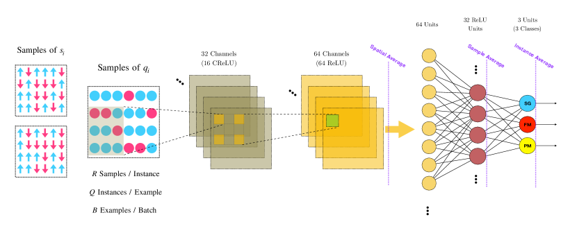
The ternary state classifying neural network (hereafter referred to as the classifier) is a three-dimensional convolutional neural network with two convolutional layers that extract spatial information from the overlap samples from each instance, followed by two fully-connected layers with intermediate averaging steps. The classifier is illustrated in Figure 1 and detailed in Algorithm 1. The predictions of the CNN for a single example manifest in line 10 as a vector $y_{i}$ of three real numbers, which are not necessarily bounded. The last step applies the “softmax” function to create probabilities

$$p_{i}=\frac{e^{y_{i}}}{\sum_{j}e^{y_{j}}}$$ (3)

that can be interpreted as the degree of belief that a given example belongs to in each class (state) $i$. We refer to these probabilities as softmax probabilities. However, the results presented here utilize a classification probability of a category $i$, which is the rate that $i$ is the most likely class (largest $p_{i}$) for the instances at a given temperature. This is the more practical measure for testing a NN.

During training we wish to align the prediction of the CNN as close as possible to the actual label of the example by adjusting the parameters of each layer of the CNN. In other words, we would like to match the softmax probabilities $p_{i}$ as close as possible with the indicator probabilities $d_{i}$, where $d_{i}=1$ if $i$ is the index of the correct state, and $0$ otherwise. This can be cast as a numerical optimization problem of a cost function $C(p_{i},d_{i})$. Here, the cost function is the negative cross entropy of the probabilities,

$$C(p_{i},d_{i})=-\sum_{i}\left[d_{i}\ln p_{i}+(1-d_{i})\ln(1-p_{i})\right].$$ (4)

The general strategy in machine learning is to calculate the numerical gradient of the cost function for a batch of examples and adjust the NN parameters in the negative gradient direction until a minimum for $C$ is reached. The simplest gradient strategy is stochastic gradient descent (SGD), where each iteration of optimization uses a random batch of examples. However, in this paper we use the ADAM Kingma and Ba (2014) method, an adaptive variant of SGD, for training the parameters of the neural network along with an $\ell^{2}$ penalty on the cost function. Further details on NN training can be found, for example, in Refs. Haykin (2008) and Goodfellow et al. (2016).

In Algorithm 1, the hyperparameters $B$, $Q$, and $R$ specify the grouping sizes of the training examples for every training step. $B$ is the number of examples in each step (the batch size), $Q$ is the number of spin-glass instances randomly selected in each example, and $R$ is number of overlap configuration samples for each instance. Per the second and third point of the design framework in Sec. II.2, a single example is a $2$-tensor of three-dimensional configurations, with dimensions $Q\times R\times L^{3}$, which is progressively reduced through the layers of the CNN into the vector $p_{i}$ of softmax probabilities. In every step of training, a batch of these examples of size $B$ is evaluated into softmax probabilities, and the cost function is averaged across the batch to evaluate the gradient of the cost function.

The convolutional layers are “pool-less,” i.e., the output tensor sizes are instead controlled through the use of kernel strides and periodic padding of the overlap samples. The primary activation function used is the rectified linear unit (ReLU) function, which simply applies $\max(x,0)$ on each element $x$ of the outgoing tensor. The first convolutional layer uses the concatenated ReLU (CReLU) variant activation function, which uses twice the number of output channels as kernels to additionally utilize the negatives of learned features. This avoids the neural network having to duplicate learning effort on closely related kernels Shang et al. (2016).

The first layer is capable of capturing correlations within a three spin radius. As the kernels have a stride of two, information redundancy is minimized while not completely decimating the spins into blocks of side length three. In the second layer, dilation Yu and Koltun (2015) introduces the capacity for the CNN to represent longer-range correlations. In our model, each individual unit in the second convolutional layer is capable of capturing correlations within a region with a side length of $7$ spins. Thus, if a large number of units in a particular channel capture the correlations they are trained to find, the spatial average is capable of expressing any long-range correlations that may be present. While deep neural networks excel at integrating such correlations for inference task, it should be advised for our particular task that they may not necessarily make use of features that are directly physically relevant after training. However, in order to successfully distinguish the SG from the FM and PM states, the neural network should at minimum be able to recognize nontrivial wave-vectors of the spin overlap, hence our inclusion of all three states in our training procedure, and our choice of basing the neural network around two convolutional layers, each with a large receptive field.

The systematic testing of models with additional layers and parameters would substantially increase the computational time and complexity of our intended objectives. Thus, the design we present here is only one possible example with the desired learning capacities, as discussed above. Adding layers and fine-tuning the model would likely increase the test accuracy, but at diminishing returns for the mere task of classifying between three possibilities.

Algorithm 1 Convolutional neural network design
                     for state classification on cubic lattices

1:procedure SG-NET-EVAL (Constants: $B$ batch size, $Q$ instances per example, $R$ overlap samples per instance; Input: $B\times Q\times R\times L^{3}$ tensor $T$ of overlap units.)

2:     Center overlap samples around the replica mean (dimension $R$).

3:     Pad all three spatial dimensions with $4-[L-1\pmod{4}]\pmod{4}$ two-dimensional slices from each opposite end (Periodic padding ensures the input spatial length $L^{\prime}$ is $1\mod 4$).

4:     Convolution 1 — $16$ CReLU activated channels (effectively $32$ output channels). Kernel length $3$. Kernel stride $2$. Output spatial length $(L^{\prime}-1)/2$.

5:     Convolution 2 — $64$ ReLU activated channels. Kernel length $2$. Dilation length $1$. Output spatial length $(L^{\prime}-1)/4$.

6:     Reduce mean over all spatial dimensions. Output tensor size $B\times Q\times R\times 64$.

7:     Fully-connected layer 1 — $32$ ReLU activated units applied on the last dimension. Output tensor size $B\times Q\times R\times 32$.

8:     Reduce mean over the overlap sample dimension. Output tensor size $B\times Q\times 32$.

9:     Fully-connected layer 2 — $3$ linear units applied on the last dimension. No bias or activation. Output tensor size $B\times Q\times 3$.

10:     Reduce mean over the instance dimension. Output tensor size $B\times 3$.

11:     Softmax and inference across the batch, where $0$ is the PM state, $1$ is the FM state, and $2$ is the SG state.

12:end procedure

II.5 Monte Carlo training sets

We use parallel tempering (PT) Monte Carlo Hukushima and Nemoto (1996) to generate spin configurations from spin-glass instances, as well as a few ferromagnet runs. Sample decorrelation is enhanced by two concurrent, independent runs of PT for each instance. Four concurrent runs are used in the case of nonzero field spin glasses. Our training procedure involves the shuffling and sampling of spin states obtained during Monte Carlo sampling. In combination with PT and training in batches of multiple instances, the trained neural network is expectedly robust against time correlations.

Table 1: Monte Carlo parameters for the instances used for training, as well as $100$ instances set aside as a validation set for the confusion method. $N$ is the number of variables, $N_{\text{sw}}$ is the number of Monte Carlo sweeps, $N_{\rm s}$ is the number of configurations taken times independent PT runs and $N_{T}$ is the number of temperatures used. EA represents the Edwards-Anderson model, FM the Ising ferromagnet.

Type	$L$	$N$	$\log_{2}N_{\text{sw}}$	$N_{\rm s}$	$N_{T}$	$[T_{\rm min},T_{\rm max}]$
EA	8	3000	22	$32\times 2$	20	[0.20, 2.00]
EA	12	600	25	$32\times 2$	20	[0.20, 2.00]
EA	12	100	25	$32\times 2$	20	[0.20, 2.00]
FM	8	1	24	$4096\times 4$	32	[2.00, 7.00]

Figure 2: Classifier accuracy as measured by Eq. (2) as the transition temperature in training is varied. An estimate of the inferred $T_{c}$ (blue square) and the Monte Carlo value found in Ref. Katzgraber et al. (2006) (red circle) are also depicted.

We generate instances for the training data as outlined in Table 1. The system size of $L=8$ is small enough to thermalize easily and thus to simulate a large number of instances, yet large enough to fit with larger systems in a finite-size scaling analysis, e.g., as done in in Ref. Katzgraber et al. (2006). A large amount of $L=8$ samples can thus provide the classifier a “big picture” view of the difference between the spin-glass state and the paramagnetic state with much more uncorrelated data. A larger system size ($L=12$) is then useful for improving the classifier’s characterization near the critical temperature. For our implementation, the size parameters of Algorithm 1, the learn rate parameter $\eta$, and the $\ell^{2}$ penalty weight parameter $\lambda$, are specified in Table 2. Error bars in classification probabilities and performance are derived from independently training the neural network $16$ times on the training instances.

Because the classifier relies on supervised training, a critical temperature needs to be presumed before labeling the data. While this could be estimated with Monte Carlo statistics or quoted from previous results, we instead utilize the confusion method introduced in Ref. van Nieuwenburg et al. (2017) to find the critical temperature. We repeat the entire training procedure for various choices of $T^{\prime}_{c}$ within the critical region, and select the choice that maximizes the accuracy of the classifier. We choose as our accuracy measure: rCl P &= ∫_T_min^T_maxd T   [ p_SG(T)θ(T’_c -T)
      +  p_PM(T)θ(T-T’_c)], where $p_{\rm SG}$ and $p_{\rm PM}$ are the classification probability densities of the SG and PM states between $T_{\rm min}$ and $T_{\rm max}$, respectively. Naturally, because data are only collected for a discrete set of temperatures, ${\mathcal{P}}$ should be calculated by a trapezoid-rule summation of the classification probabilities divided by the temperature interval measure $T_{\rm min}-T_{\rm max}$. It is important to weigh the classification probabilities as a numerical integral–and not just sum them directly–to take the uneven spacing of the simulation temperatures into account.

Figure 3: Classification probabilities of the CNN for finding a spin glass (SG) or paramagnetic (PM) state. Where the probabilities do not add up to $1$, the remainder belongs to FM classification probability, which is omitted for clarity. The figure inset zooms into the region between $T=0.85$ and $T=1.05$ where the transition in classification probability occurs for better visibility.

To simplify training, the critical temperature for classifying the FM state is simply quoted as $T_{c}=4.51$ Binder and Luijten (2001). We do not attempt to optimize this transition temperature with the confusion method.

Table 2: Training parameters for the neural network. Training is divided into three stages where the parameters are adjusted for the specified amount of steps. $\eta$ represents the learn rate parameter, $\lambda$ the penalty weight parameter, $B$ is the number of examples, and $Q$ and $R$ specify the grouping sizes for the training examples for each training step.

Steps	$\eta$	$\lambda$	$B$	$Q$	$R$
2000	$10^{-3}$	$0.005$	12	6	16
4000	$10^{-4}$	$0.005$	12	6	16
4000	$10^{-5}$	$0$	12	6	16

III Results

Table 3: Table of parameters for each instance class simulated for a given linear size $L$ and field strength $h$ for the test set of examples. See Table 1 for additional details.

$L$	$h$	$N$	$\log_{2}N_{\text{sw}}$	$N_{s}$	$N_{T}$
6	0	1000	23	64	20
8	0	400	23	128	20
10	0	400	24	64	20
12	0	100	25	64	20
10	0.025	500	24	64	16
6	0.05	500	23	64	16
8	0.05	500	23	64	16
10	0.05	500	24	64	16
10	0.075	500	24	64	16
6	0.10	500	24	64	16
8	0.10	500	24	64	16
10	0.10	500	24	64	16

III.1 Confusion ensemble

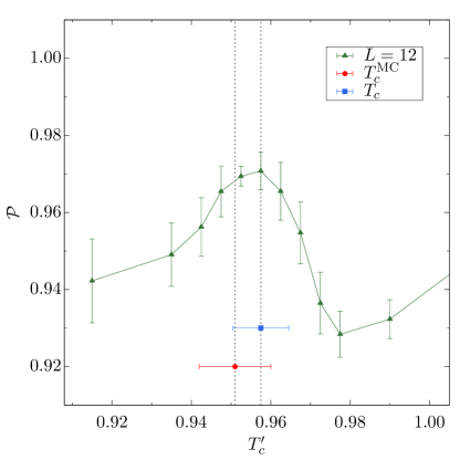
The confusion method is carried out with a validation set of $100$ spin-glass instances with $L=12$, which were not used for training the classifier. The average accuracy as a function of $T^{\prime}_{c}$ shown in Fig. 2. The accuracy peak suggests a transition temperature of approximately $T_{c}=0.958(8)$. This is consistent with the critical temperature of the Edwards-Anderson model with Gaussian disorder as found, for example, in Ref. Katzgraber et al. (2006). The precise temperatures used as the boundary between the PM and SG states that are within the range of both $T_{c}$ values are $0.953$ and $0.958$. In the figures that follow, we use the classifier model trained at $T^{\prime}_{c}=0.953$, however, the results from either model are practically identical.

The configuration samples for testing the classifier are obtained with parallel tempering Monte Carlo simulations, with parameters listed in Table 3. For spin glasses in a field, we use the same temperature range and at least 10 times the number of sweeps as Ref. Young and Katzgraber (2004) used up to $L=8$ to ensure termalization. The samples are collected after a thermalization period of 75% of the sweeps, for a time between samples of $2^{16}$ sweeps.

III.2 Spin glasses at zero field

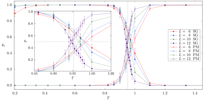
Figure 3 shows the classification probabilities of the classifier evaluated on the sample of spin-glass test instances. In all figures, vertical dashed lines represent transition temperatures and horizontal dashed lines the 50% probability line. The classification probabilities follow a smooth transition near the critical temperature. The classifier performs well, except for an anomalous jump in FM classification at the lowest temperature. This is likely due to the possibility of sampling instances with simple energy landscapes when dealing with finite-size spin glasses. This is supported by observing the finite size behavior as $L$ increases to $12$, for which the FM anomaly vanishes.

III.3 Ferromagnetic classification probabilities

Figure 4: Classification probabilities for the three-dimensional Ising ferromagnet. Although finite-size effects are visible, these data are only used to illustrate the detection of the FM state.

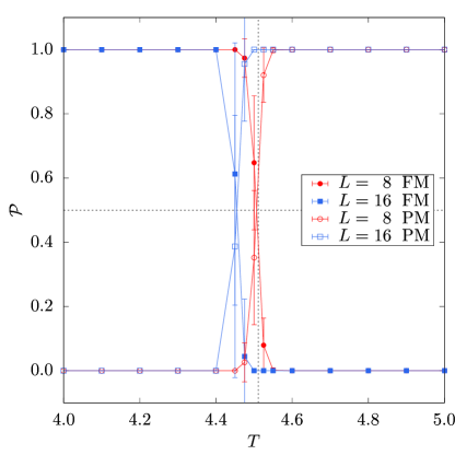
Figure 4 shows the classification probabilities of the classifier on a test set of three-dimensional Ising ferromagnet samples Note that in the CNN algorithm, the instance averaging step is kept for code consistency. An “instance” of the Ising ferromagnet is simply another set of uncorrelated configuration samples. The distinction that the classifier learns is affected by finite-size effects, i.e., the labeling that the classifier learns for $L=8$ ($T^{\prime}_{c}=4.51$) shifts for $L=16$ ($T^{\prime}_{c}=4.46$) to a lower value. Observables that would diverge at the phase transition, such as heat capacity, in the thermodynamic limit are instead critical at higher temperatures for small system sizes. The shift away from $T_{c}$ at system sizes larger the training set is expected since the larger system sizes become critical at slight lower temperature than the smallest system size. This causes the predicted transition of a larger system to seem lower than the learned representation.

The classifier’s sharp transition region is likely a consequence of the number of available training parameters in the model, compared to the complexity of the learning task of distinguishing between the PM and FM states on a given system size, as well as the enhancement furnished by averaging over multiple configuration samples.

In principle, the characteristics of these classification probabilities may be useful as a NN-based finite-size scaling technique. However, neither learning the three-dimensional Ising ferromagnetic transition temperature to high precision nor inferring its critical properties from the NN were initial objectives in this work.

III.4 Generalization to bimodal disorder

Figure 5: Classification probabilities of CNN trained on the Edwards-Anderson spin glass with Gaussian disorder with a test set of instances with bimodal disorder. The data cross close to $T^{\prime}_{c}\approx 1.1$, the known value of the bimodal spin-glass transition temperature.

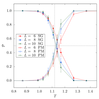
As a first generalization test, we generate a test set of spin-glass instances with bimodal instead of Gaussian disorder. In this case, the critical temperature shifts to $T_{c}\approx 1.12$ Katzgraber et al. (2006). The crossover point easily shifts to this new temperature. We take this as very good evidence that the classifier learns a good representation of the spin-glass state, and can make accurate predictions for different spin-glass models with different disorder distributions.

III.5 Generalization to nonzero fields

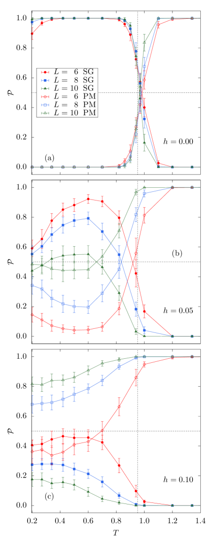
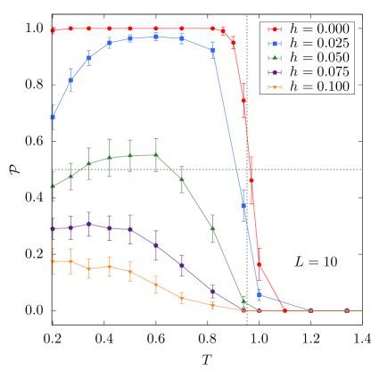
Now that we have demonstrated that our NN can detect a spin-glass transition at zero field and even detect correct transition temperatures when the disorder is changed, we evaluate its prediction for a spin-glass state in a field. The classification probabilities for nonzero fields are shown in Figure 6. It can be observed that at $h=0.05$, the spin-glass signal for the classifier becomes weak. At a stronger field, $h=0.10$, the PM phase becomes dominant with larger linear system sizes $L$. Figure 7 illustrates a break down of any crossing temperature beyond system sizes of $L=6$.

We emphasize again that the model is trained under the limitations explained for the framework, and the system sizes examined here may not be conclusive in the thermodynamic limit. However, at least for the system sizes examined here, we can observe that the transition from the spin-glass state to the PM state with increasing $h$ becomes sharper as the system size is increased. From this trend, one would conclude from the results of the classifier that if there is a spin-glass state in a field, it occurs for fields $h\lesssim 0.05$. This is consistent with the correlation length-based analysis of Ref. Young and Katzgraber (2004) for similar system sizes.

Figure 6: Progression of classification probabilities for different fields. As the field increases, the SG signal weakens progressively. Even for fields as weak as $h=0.05$ the signal of the transition moves to zero temperature as the system size increases. Data for (a) $h=0.00$, (b) $h=0.05$, and (c) $h=0.10$.

Figure 7: Progression of classification probabilities with increasing field for $L=10$. The stronger the field, the weaker the signal for a SG state.

IV Summary and conclusion

We have implemented and evaluated an input-size agnostic three-dimensional convolutional neural network for ternary phase classification on Ising-like models three-dimensional cubic lattice and found evidence that such a neural network can acquire an accurate representation of the spin-glass state at zero field. We emphasize that performing this classification task is nontrivial, because of the lack of spatial magnetic order in these systems. Furthermore, the approach can be generalized to other three-dimensional models.

Conditioned on training at zero field only, the classification inference of the neural network at nonzero field would suggest that a spin-glass state in a field might not be stable for three-dimensional systems. This inference comes with the caveats discussed above. Most significantly there is no a priori theoretical reason to expect the neural network’s accuracy on data sets of a significantly different nature to be high. As such, phase-classifying neural networks are by no means intended to replace or directly compare with Monte Carlo sampling of observables, and have utility instead as a cost-effective, qualitative guide for exploring the phase space of condensed matter systems outside of well-studied regimes. We emphasize that the numerical effort needed for the learning and classification tasks here can be made considerably small: Whereas most spin-glass studies require tens of thousands of samples at nonzero field, with the neural network a likely conclusion can be drawn from as little as $500$ disorder instances, and at minimum helps to identify the relevant energy scale for the nonzero field. Suppression of rare sample could further improve the economy of machine learning methods for spin glasses in a field.

In specific renormalization group (RG) terms, the neural network has built in a particular representation for the RG flow for only the SG, FM, and PM states for a spin-glass model at zero field after training, and by assumption excludes the possibility of an additional fixed point to cause an additional state for the neural network to consider. While this would indeed cast the qualitative validity of the neural network’s predictions at nonzero field into question, we believe that this is a very unlikely scenario for three-dimensional spin glasses where our results agree qualitatively with multiple numerical studies in the literature Caracciolo et al. (1990); Houdayer and Martin (1999); Young and Katzgraber (2004); Katzgraber and Young (2005); Sasaki et al. (2007); Jörg et al. (2008); Katzgraber et al. (2009a); Larson et al. (2013). Adapting our framework to design neural networks for higher-dimensional and long-range spin glass models is an important future step in concretely establishing the range and utility of machine learning in equilibrium spin glass physics.

In general, NNs once optimized could be used to probe the phase characteristics of modified spin-glass models where Monte Carlo statistics may happen to be unavailable or inconclusive. Examples are systems where no local order parameter exists, such as in lattice gauge theories found for some error models when determining error thresholds for topological codes Dennis et al. (2002); Arakawa et al. (2005); Katzgraber et al. (2009b); Andrist et al. (2011); Bombin et al. (2012); Andrist et al. (2012).

Further computational and theoretical research in this disciplinary interface may be encouraging. Both neural networks and spin glasses are examples of complex systems with a breadth of applications, where in fact some neural networks can find a description though long-range spin glasses Nishimori (2001). The converse study of describing spin glasses through neural networks may prove rewarding from the point of view of complexity theory.

V Acknowledgments

We would like to thank Amin Barzegar, Chao Fang and Evert van Nieuwenburg for comments and useful discussions. H. M. B. acknowledges financial support from the Marianne ’76 and Robert ’77 Hamm Endowed Scholarship from the Department of Physics and Astronomy while a student at Texas A&M University. The research of H. M. B. is based upon work (partially) supported by the Office of the Director of National Intelligence (ODNI), Intelligence Advanced Research Projects Activity (IARPA), via the U.S. Army Research Office contract W911NF-17-C-0050. H. G. K. acknowledge support from the National Science Foundation (Grant No. DMR-1151387). The work of H. G. K. is supported in part by the Office of the Director of National Intelligence (ODNI), Intelligence Advanced Research Projects Activity (IARPA), via MIT Lincoln Laboratory Air Force Contract No. FA8721-05-C-0002. The views and conclusions contained herein are those of the authors and should not be interpreted as necessarily representing the official policies or endorsements, either expressed or implied, of ODNI, IARPA, or the U.S. Government. The U.S. Government is authorized to reproduce and distribute reprints for Governmental purpose notwithstanding any copyright annotation thereon. We thank Texas A&M University for access to their Ada and Terra clusters.

References

- Haykin (2008) S. O. Haykin, Neural Networks and Learning Machines (Pearson, 2008).
- Goodfellow et al. (2016) I. Goodfellow, Y. Bengio, and A. Courville, Deep Learning (MIT Press, 2016), http://www.deeplearningbook.org.
- Bishop (2006) C. Bishop, Pattern Recognition and Machine Learning (Springer-Verlag, New York, 2006).
- Carrasquilla and Melko (2017) J. Carrasquilla and R. G. Melko, Machine learning phases of matter, Nature Physics 13, 431 (2017).
- Ch’ng et al. (2017) K. Ch’ng, J. Carrasquilla, R. G. Melko, and E. Khatami, Machine Learning Phases of Strongly Correlated Fermions, Phys. Rev. X 7, 031038 (2017).
- Tanaka and Tomiya (2017) A. Tanaka and A. Tomiya, Detection of Phase Transition via Convolutional Neural Networks, J. Phys. Soc. Jpn 86, 063001 (2017).
- Kashiwa et al. (2018) K. Kashiwa, Y. Kikuchi, and A. Tomiya, Phase Transition Encoded in Neural Network (2018), (arxiv:cond-mat/1812.01522).
- Ronhovde et al. (2011) P. Ronhovde, S. Chakrabarty, D. Hu, M. Sahu, K. K. Sahu, K. F. Kelton, N. A. Mauro, and Z. Nussinov, Detection of Hidden Structures on All Scales in Amorphous Materials and Complex Physical Systems: Basic Notions and Applications to Networks, Lattice Systems, and Glasses, The European Physical Journal E 34, 105 (2011).
- Nussinov et al. (2016) Z. Nussinov, P. Ronhovde, D. Hu, S. Chakrabarty, B. Sun, N. A. Mauro, and K. K. Sahu, Inference of Hidden Structures in Complex Physical Systems by Multi-Scale Clustering, in Information Science for Materials Discovery and Design, edited by T. Lookman, F. J. Alexander, and K. Rajan (Springer International Publishing, Cham, 2016), Springer Series in Materials Science, p. 115.
- Binder and Young (1986) K. Binder and A. P. Young, Spin Glasses: Experimental Facts, Theoretical Concepts and Open Questions, Rev. Mod. Phys. 58, 801 (1986).
- Mézard et al. (1987) M. Mézard, G. Parisi, and M. A. Virasoro, Spin Glass Theory and Beyond (World Scientific, Singapore, 1987).
- Young (1998) A. P. Young, ed., Spin Glasses and Random Fields (World Scientific, Singapore, 1998).
- Stein and Newman (2013) D. L. Stein and C. M. Newman, Spin Glasses and Complexity, Primers in Complex Systems (Princeton University Press, Princeton NJ, 2013).
- Parisi (1980) G. Parisi, The order parameter for spin glasses: a function on the interval –, J. Phys. A 13, 1101 (1980).
- Fisher and Huse (1986) D. S. Fisher and D. A. Huse, Ordered phase of short-range Ising spin-glasses, Phys. Rev. Lett. 56, 1601 (1986).
- Fisher and Huse (1988) D. S. Fisher and D. A. Huse, Equilibrium behavior of the spin-glass ordered phase, Phys. Rev. B 38, 386 (1988).
- Moore and Bray (2011) M. A. Moore and A. J. Bray, Disappearance of the de Almeida-Thouless line in six dimensions, Phys. Rev. B 83, 224408 (2011).
- Moore (2012) M. A. Moore, expansion in spin glasses and the de Almeida-Thouless line, Phys. Rev. E 86, 031114 (2012).
- Caracciolo et al. (1990) S. Caracciolo, G. Parisi, S. Patarnello, and N. Sourlas, 3d Ising spin-glasses in a magnetic field and mean-field theory, Europhys. Lett. 11, 783 (1990).
- Houdayer and Martin (1999) J. Houdayer and O. C. Martin, Ising spin glasses in a magnetic field, Phys. Rev. Lett. 82, 4934 (1999).
- Young and Katzgraber (2004) A. P. Young and H. G. Katzgraber, Absence of an Almeida-Thouless line in Three-Dimensional Spin Glasses, Phys. Rev. Lett. 93, 207203 (2004).
- Katzgraber and Young (2005) H. G. Katzgraber and A. P. Young, Probing the Almeida-Thouless line away from the mean-field model, Phys. Rev. B 72, 184416 (2005).
- Sasaki et al. (2007) M. Sasaki, K. Hukushima, H. Yoshino, and H. Takayama, Scaling Analysis of Domain-Wall Free Energy in the Edwards-Anderson Ising Spin Glass in a Magnetic Field, Phys. Rev. Lett. 99, 137202 (2007).
- Jörg et al. (2008) T. Jörg, H. G. Katzgraber, and F. Krzakala, Behavior of Ising Spin Glasses in a Magnetic Field, Phys. Rev. Lett. 100, 197202 (2008).
- Katzgraber et al. (2009a) H. G. Katzgraber, D. Larson, and A. P. Young, Study of the de Almeida-Thouless line using power-law diluted one-dimensional Ising spin glasses, Phys. Rev. Lett. 102, 177205 (2009a).
- Larson et al. (2013) D. Larson, H. G. Katzgraber, M. A. Moore, and A. P. Young, Spin glasses in a field: Three and four dimensions as seen from one space dimension, Phys. Rev. B 87, 024414 (2013).
- Marinari et al. (1998) E. Marinari, G. Parisi, and J. Zuliani, Four-dimensional spin glasses in a magnetic field have a mean-field-like phase, J. Phys. A 31, 1181 (1998).
- Leuzzi et al. (2009) L. Leuzzi, G. Parisi, F. Ricci-Tersenghi, and J. J. Ruiz-Lorenzo, Ising Spin-Glass Transition in a Magnetic Field Outside the Limit of Validity of Mean-Field Theory, Phys. Rev. Lett. 103, 267201 (2009).
- Fernández (2010) J. F. Fernández, Evidence against an Almeida-Thouless line in disordered systems of Ising dipoles, Phys. Rev. B 82, 144436 (2010).
- Baity-Jesi et al. (2014) M. Baity-Jesi, R. Alvarez Baños, A. Cruz, L. A. Fernandez, J. M. Gil-Narvion, Gordillo-Guerrero, D. Iñiguez, A. Maiorano, F. Mantovani, E. Marinari, et al., Dynamical transition in the Edwards-Anderson spin glass in an external magnetic field, Phys. Rev. E 89, 032140 (2014).
- Angelini and Biroli (2015) M. C. Angelini and G. Biroli, Spin Glass in a Field: A New Zero-Temperature Fixed Point in Finite Dimensions, Phys. Rev. Lett. 114, 095701 (2015).
- de Almeida and Thouless (1978) J. R. L. de Almeida and D. J. Thouless, Stability of the Sherrington-Kirkpatrick solution of a spin glass model, J. Phys. A 11, 983 (1978).
- Newman and Stein (2007) C. M. Newman and D. L. Stein, Short-range spin glasses: Results and speculations, in Lecture Notes in Mathematics 1900 (Springer-Verlag, Berlin, 2007), p. 159, (cond-mat/0503345).
- Abadi et al. (2016) M. Abadi et al., TensorFlow: A System for Large-Scale Machine Learning (2016), http://tensorflow.org.
- Edwards and Anderson (1975) S. F. Edwards and P. W. Anderson, Theory of spin glasses, J. Phys. F: Met. Phys. 5, 965 (1975).
- Yeomans (1992) J. M. Yeomans, Statistical Mechanics of Phase Transitions (Oxford University Press, Oxford, 1992).
- Baity-Jesi et al. (2014) M. Baity-Jesi, R. A. Baños, A. Cruz, L. A. Fernandez, J. M. Gil-Narvion, A. Gordillo-Guerrero, D. Iñiguez, A. Maiorano, F. Mantovani, E. Marinari, et al., The three-dimensional Ising spin glass in an external magnetic field: the role of the silent majority, J. Stat. Mech. P05014 (2014), (arXiv:cond-mat/1101.2646).
- Parisi and Temesvári (2012) G. Parisi and T. Temesvári, Replica symmetry breaking in and around six dimensions, Nuc. Phys.B 858, 293 (2012).
- Baños et al. (2012) R. A. Baños, A. Cruz, L. A. Fernandez, J. M. Gil-Narvion, A. Gordillo-Guerrero, M. Guidetti, D. Iñiguez, A. Maiorano, E. Marinari, V. Martin-Mayor, et al., Thermodynamic glass transition in a spin glass without time-reversal symmetry, Proc. Natl. Acad. Sci. U.S.A. 109, 6452 (2012).
- Kingma and Ba (2014) D. P. Kingma and J. Ba, Adam: A Method for Stochastic Optimization (2014), (arXiv:1412.6980).
- Shang et al. (2016) W. Shang, K. Sohn, D. Almeida, and H. Lee, Understanding and Improving Convolutional Neural Networks via Concatenated Rectified Linear Units, International Conference on Machine Learning p. 2217 (2016), (arXiv:1603.05201).
- Yu and Koltun (2015) F. Yu and V. Koltun, Multi-scale context aggregation by dilated convolutions (2015).
- Hukushima and Nemoto (1996) K. Hukushima and K. Nemoto, Exchange Monte Carlo method and application to spin glass simulations, J. Phys. Soc. Jpn. 65, 1604 (1996).
- Katzgraber et al. (2006) H. G. Katzgraber, M. Körner, and A. P. Young, Universality in three-dimensional Ising spin glasses: A Monte Carlo study, Phys. Rev. B 73, 224432 (2006).
- van Nieuwenburg et al. (2017) E. P. L. van Nieuwenburg, Y.-H. Liu, and S. D. Huber, Learning phase transitions by confusion, Nat. Phys. 13, 435 (2017).
- Binder and Luijten (2001) K. Binder and E. Luijten, Monte carlo tests of renormalization-group predictions for critical phenomena in ising models, Phys. Rep 344, 179 (2001).
- Dennis et al. (2002) E. Dennis, A. Kitaev, A. Landahl, and J. Preskill, Topological quantum memory, J. Math. Phys. 43, 4452 (2002).
- Arakawa et al. (2005) G. Arakawa, I. Ichinose, T. Matsui, and K. Takeda, Self-duality and phase structure of the 4D random-plaquette gauge model, Nucl. Phys. B 709, 296 (2005).
- Katzgraber et al. (2009b) H. G. Katzgraber, H. Bombin, and M. A. Martin-Delgado, Error Threshold for Color Codes and Random 3-Body Ising Models, Phys. Rev. Lett. 103, 090501 (2009b).
- Andrist et al. (2011) R. S. Andrist, H. G. Katzgraber, H. Bombin, and M. A. Martin-Delgado, Tricolored Lattice Gauge Theory with Randomness: Fault-Tolerance in Topological Color Codes, New J. Phys. 13, 083006 (2011).
- Bombin et al. (2012) H. Bombin, R. S. Andrist, M. Ohzeki, H. G. Katzgraber, and M. A. Martin-Delgado, Strong Resilience of Topological Codes to Depolarization, Phys. Rev. X 2, 021004 (2012).
- Andrist et al. (2012) R. S. Andrist, H. Bombin, H. G. Katzgraber, and M. A. Martin-Delgado, Optimal error correction in topological subsystem codes, Phys. Rev. A 85, 050302 (2012).
- Nishimori (2001) H. Nishimori, Statistical Physics of Spin Glasses and Information Processing: An Introduction (Oxford University Press, New York, 2001).