A super-Earth and two sub-Neptunes transiting the nearby and quiet M dwarf TOI-270

One of the primary goals of exoplanetary science is to detect small, temperate planets passing (transiting) in front of bright and quiet host stars. This enables the characterisation of planets’ sizes, orbits, bulk compositions, atmospheres and formation histories. These studies are further favoured by small and cool M dwarf hosts. Here, we report the Transiting Exoplanet Survey Satellite discovery of three small planets transiting one of the nearest and brightest M dwarf hosts to date, TOI-270 (TIC 259377017; K-mag 8.3; 22.5 parsec). The M3V-type star is transited by the super-Earth-sized TOI-270 b ($1.247_{-0.083}^{+0.089}$ R_⊕) and the sub-Neptune-sized TOI-270 c ($2.42\pm 0.13$ R_⊕) and TOI-270 d ($2.13\pm 0.12$ R_⊕). The planets orbit close to a mean-motion resonant chain, with periods ($3.36$, $5.66$, and $11.38$ days) near ratios of small integers ($5:3$ and $2:1$). TOI-270 is a prime target for future studies since: 1) its near-resonance allows detecting transit timing variations for precise mass measurements and dynamical studies; 2) its brightness enables independent radial velocity mass measurements; 3) the outer planets are ideal for atmospheric characterisation via transmission spectroscopy; and 4) the quiet star enables future searches for habitable zone planets. Altogether, very few systems with small, temperate exoplanets are as suitable for such complementary and detailed characterisation as TOI-270.

The super-Earth-sized and two sub-Neptune-sized planets transiting TOI-270 were detected by the Transiting Exoplanet Survey Satellite (TESS) mission in Sectors 3–5 (Fig. 1), and followed up with ground-based multi-wavelength photometry, reconnaissance spectroscopy, and high resolution imaging. Following an extensive vetting protocol including these observations and archival/catalogue data, we validate the transit signals to be of planetary origin and the host to be a single $\mathrm{M}3.0\pm 0.5\mathrm{V}$ star (see Methods). With a distance of only 22.5 parsec, TOI-270 is one of the closest transiting exoplanet hosts to Earth (Fig 2). We find a stellar mass of $0.40\pm 0.02$ M_⊙, radius of $0.38\pm 0.02$ R_⊙, effective temperature of $3386_{-131}^{+137}$ K, and metallicity of $-0.17\pm 0.1$ from empirical relations (see Methods; Table 1), and detect low magnetic activity indicated by the presence of an H_α absorption line in the stellar spectrum.

The three exoplanets are among the smallest and nearest transiting exoplanets known to date (Fig. 2). The radius of TOI-270 b places it in a planetary population distinct from planets c and d; the trio is separated by the planetary radius gap around 1.7–2.0 R_⊕ which divides two populations of planets, rocky super-Earths and gas-dominated sub-Neptunes (e.g. [1, 2, 3]; Fig. 2). TOI-270 b likely falls into the regime of Earth-like/rocky compositions, while planets c and d are possibly water-ice or gas-dominated sub-Neptunes when employing statistically predicted masses of $1.9^{+1.5}_{-0.7}$ M_⊕, $6.6^{+5.2}_{-2.8}$ M_⊕, and $5.4^{+4.0}_{-2.1}$ M_⊕, respectively ([21, 3, 22]; Fig. 2). The diversity of the TOI-270 system thus provides an interesting case study for planet formation and photoevaporation, which can be driven by future observations using transit timining variations (TTVs), radial velocities (RVs) and transmission spectroscopy (discussed below).

Since the planets orbit near a resonant configuration, one can expect to measure TTVs - and thus planet masses - in the near future. The proximity to the 2:1 resonance for TOI-270 c and d suggests that their perturbations lead to significant TTVs for both planets. If the inner planet pair (near 5:3 resonance) has a high relative eccentricity, it could also lead to observable TTVs for planet b. However, given the available observation span of the TESS and follow-up data ($\sim$120 days), and the transit timing uncertainty ($\sim$2–5 minutes), TOI-270 is still best described as a multi-planet system on circular orbits with constant periods; we find no strong Bayesian evidence for eccentricity nor for TTVs (Supplementary Table 2). We thus assess the theoretically expected amplitude and super-period of the TTVs through 4-body simulations [6]. We find that the current observation span samples only a short and approximately linear part of the full TTV signal, which has a super-period of 1000-1100 days (Fig. 3). The TTV amplitudes of planets c and d are expected to be $\gtrsim 10$ min. and $\gtrsim 30$ min., respectively. These are approximate lower limits, as the planet masses are currently predicted rather than measured, and the orbits are assumed to be circular. Dynamical stability simulations show that the system is exceedingly stable for a range of eccentricities and planetary masses (see Supplementary Information), opening the possibility of non-circular orbits and even higher densities (and thus even larger TTVs). Future transit observations sampling the super-period with moderate time-precision ($\sim$ few min.) should thus be sufficient to determine the TTV signal. Importantly, the bias in predicting future transits from the linear ephemerides fit increases rapidly. For example, after just one year, planet d will have a systematic transit window offset by $>1$ hour due to the dynamical interactions. All this motivates the need for a continuous follow-up campaign, with observations every few months over the next 1–2 years.

Moreover, TOI-270 is inactive and much brighter than most comparable multi-planet hosts (especially in the infrared), making it a good target for precise radial velocity measurements with HARPS or ESPRESSO. We expect RV semi-amplitudes of around 2, 5, and 3 m/s for planets b, c, and d, given the predicted masses. This opens up the potential for accurate determination of the planets’ masses and eccentricities in an independent and complementary way to TTV studies. The majority of comparable multi-planet systems discovered by Kepler are too faint for RV follow-up (although K2 improved this situation to some degree). Only few bright-enough systems comparable to TOI-270 are known, such as K2-3 [7], K2-18 [8], and LHS 1140 [9]. However, these and most Kepler systems are not as close to resonances, even when they do feature planets with similar sizes and orbital spacings [10]. Consequently, very few other multi-systems with small planets are as suitable as TOI-270 for complementary characterisation by both TTVs and RVs. This ultimately will provide insights into both the compositions and formations of three very interesting planets, which can be representative for compact multi-planet systems around M dwarfs.

As one of the nearest (and hence brightest) M dwarf systems with transiting exoplanets, TOI-270 is also a promising target for atmospheric characterisation studies. The low equilibrium temperatures of planets c and d ($424_{-19}^{+20}$ K and $340\pm 14$ K) make them rare objects among currently known transiting super-Earth-sized and sub-Neptune-sized planets, and thus additionally compelling. Further, TOI-270 will be observable with the James Webb Space Telescope (JWST) for 215 days per year, allowing easy observation scheduling. Absorption features of planets c and d are expected to be readily detectable with $\mathrm{SNR}>40$ and $\mathrm{SNR}>60$, respectively, from just one transit with the NIRISS instrument and assuming cloud-free and H₂-dominated atmospheres [11, 12]. Hence, TOI-270 provides a rare opportunity to test whether planets in compact multi-planet systems share the same formation history by comparing the atmospheric composition and thickness [13, 14]. Moreover, it could be possible to constrain the ocean loss on these planets, by uniting the red-sensitive JWST observations (probing $O_{3}$ abundances) with ground-based, visible-spectrum observations from the Extremely Large Telescopes (probing $O_{2}$ abundances; e.g. [15, 16]). Alternatively, one could search for $CO$ and $O_{4}$ features as indicators [17].

The equilibrium temperature of TOI-270 d also places the planet within the survivable range of temperatures for extremophile organisms (Fig. 1, [18]). This temperate small exoplanet can thus be a unique laboratory, being exceptionally suited for characterisation by TTVs, RVs and transmission spectroscopy. While planet d itself might not be rocky and potentially too massive for habitable oceans [19], plus it might suffer from runaway greenhouse effects and extreme water loss [15], it could host temperate rocky moons (see e.g. [20]). Additional companions beyond the orbit of TOI-270 d could also fall within the terrestrial-like habitable zone (0.10–0.28 AU [25]) without impacting the stability of the system (see Supplementary Information). Such planets are not expected to be detectable in the current data alone, encouraging future exploration (see Methods; Supplementary Fig. 7). The host star, TOI-270, is remarkably well suited for future habitability searches, as it is particularly quiet for an M dwarf (e.g. [22]); it shows no signs of rotational variability, spots or stellar flares during our photometric observations, and low H-alpha activity in the reconnaissance spectra. This makes it an ideal target for radial velocity surveys searching for additional planets in the habitable zone [23]. Moreover, the star is unlikely to sterilise or diminish the atmospheres of its planets through flaring or coronal mass ejections at its current stage (e.g. [24, 25, 26]; note that the star might have been more active at a younger age).

We note two caveats: first, tidal effects can substantially influence localised habitability, which is not included in any terrestrial-like habitable zone definition. In fact, due to the short orbital distances of the three planets, the planets rotation is expected to be tidally locked to their orbits. Using dynamical simulations including planetary tides, we find that the obliquities decrease down to zero and all planetary rotation periods evolve towards pseudo-synchronisation in a timescale shorter than 10⁵ years (see Supplementary Information). The second caveat is that the equilibrium temperature is not necessarily reflective of the surface temperature – follow-up studies investigating the bulk masses, tidal locking, atmospheric compositions and pressures, and recirculation of gas and/or liquid water are required to determine any surface habitability. Nevertheless, the TOI-270 system stands representative for a demographic of exoplanets in the potential habitable zone of M dwarfs, paving the way for future habitable zone planet discoveries with TESS.

Compact multi-planet systems like TOI-270 are often accompanied by other small planets on short orbits. For example, this was the case for TRAPPIST-1, whose initial three planet signals were later found to be part of a seven planet resonance chain [27]. We thus perform a search for additional components, and identify two more signals with a signal-to-noise ratio $\mathrm{SNR}>5$ (see Methods; Supplementary Table 4). However, after inspecting the data, we suggest that these are likely not planets but systematic artefacts. Nevertheless, long-period or non-transiting companions might accompany the planet trio, and could be detected with follow-up monitoring.

Soon, we will be able to precisely measure the masses of TOI-270 c and d through photometric follow-up of the significant TTVs caused by the multi-planet dynamics, and, independently, through RV observations enabled by the star’s brightness and quietness. TOI-270 thus provides three new exoplanets which soon will fulfil the primary goal of the TESS mission (detecting and measuring the masses of at least 50 planets smaller than Neptune). Even more, we will be able to study the atmospheric composition of TOI-270’s planets via transmission spectroscopy with JWST and the ELTs with high SNR and near-optimal visibility. Falling on both sides of the planet radius gap, the formation of these three interesting planets is likely representative of many other systems. All follow-up studies together (TTVs, RVs and transmission spectroscopy) will give insight into the bulk and atmospheric compositions of the planets, and provide an interesting case study for formation and photoevaporation. Finally, with planet d falling into a temperate regime, and potentially more planets waiting to be discovered in the habitable zone, TOI-270 could provide an exemplary case for exoplanet habitability studies in the future.

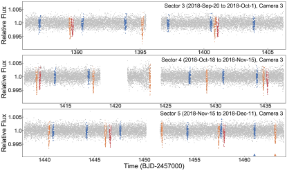
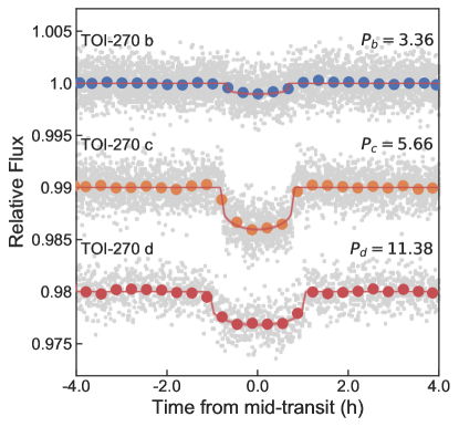
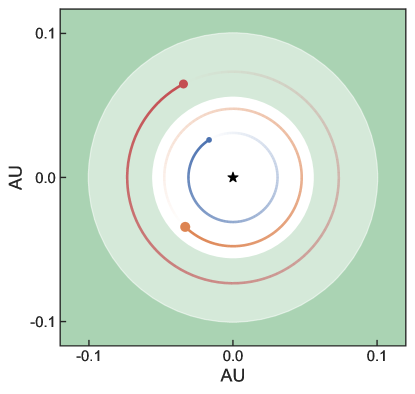
Figure 1: The discovery data and orbits of the super-Earth and two sub-Neptunes transiting TOI-270. Top: the full TESS discovery lightcurve of Sectors 3, 4 and 5 (grey points), with transits of planets b (blue), c (orange) and d (red) marked in colour. Lower left: TESS lightcurves phase-folded onto the best-fit periods for all three planets. Grey points show the individual 2 min. cadence observations, coloured circles show the data binned in phase with 15 min. spacing. Red lines show 20 lightcurve models generated from randomly drawn posterior samples by the allesfitter analysis ([28]; see Methods). Lower right: a top-down view of the system. The dark-green area shows the optimistic habitable zone according to [25], spanning 0.10 AU to 0.28 AU. The light-green area shows the orbital distance at which the equilibrium temperature of a planet is between the survival temperature for extremophiles ($\sim$395 K) [18] and the freezing point of water (273.15 K), spanning 0.06 AU to 0.12 AU. Note that the equilibrium temperature can differ from the surface temperature.

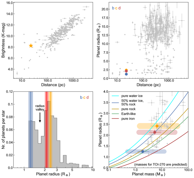
Figure 2: TOI-270 in the context of known exoplanets. Top left: the brightness (as 2MASS K-band magnitude) versus the distance to Earth (in parsec) of the TOI-270 host star (orange star symbol), compared with known exoplanet hosts (grey circles with 68.3% credible intervals). Top right: the planet radii versus the system’s distance to Earth, shown for TOI-270 b, c and d (blue, orange and red circles, respectively) compared with known exoplanets (grey circles with 68.3% credible intervals). Bottom left: a histogram of the number of planets per star (for orbital periods $<100$ days) over planet radius, as reported by [1]. The radii of TOI-270 b, c and d are marked for comparison (blue, orange, and red lines; coloured bands showing 68.3% credible intervals). The radius valley appears around 1.7–2.0 R_⊕ separating two populations of planets, rocky super-Earths and gas-dominated sub-Neptunes (e.g. [3]). Bottom right: mass-radius-diagram indicating the potential bulk compositions of the three TOI-270 planets and known exoplanets. The TOI-270 masses are predicted from the relations of [22], with the 68.3% and 99.7% credible intervals of the predictions shown as lines and bands, respectively. Overplotted are theoretical bulk composition curves from [21] (water/ice: $\mathrm{H_{2}O}$; rock: $\mathrm{Mg2SiO4}$; iron: $\mathrm{Fe}$; Earth-like: 67% rock / 33% iron), and a comparison with known exoplanets (grey circles with 68.3% credible intervals). In all panels, the data on known exoplanets is from https://exoplanetarchive.ipac.caltech.edu/, online 2019 March 04. Only known transiting exoplanets with values measured to better than a 30% relative error are shown. These four views highlight how TOI-270 occupies an exciting parameter space for future studies, with the diversity of the system providing an interesting case study for planet formation and photoevaporation.

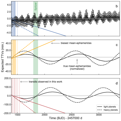
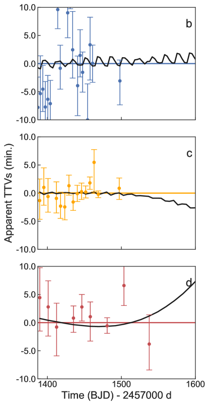
Figure 3: Expected and apparent transit timing variations (TTVs) of the TOI-270 system. Left: Expected TTVs of the TOI-270 system, assuming the true mean-ephemerides of the system were known. Two example simulations show ‘light planets’ (solid black lines) with masses predicted from [22] and ‘heavy planets’ (dashed black lines) composed of 50% water ice and 50% rock [29]. A future Spitzer observation window is marked in green. The expected TTVs have amplitudes of $\gtrsim 10$ min. (planet c) and $\gtrsim 30$ min. (planet d) and super-periods of 1000–1100 days. However, the current observations (coloured vertical lines) span only a short, approximately linear part of the TTV signal, biasing mean-ephemerides fits (dashed and solid coloured lines). Right: Apparent TTVs when the mean-ephemerides are predicted from only the observed transits (and thus biased). Coloured error bars show TTVs and 68.3% credible intervals from the best-fit model, coloured lines show the best-fit mean-ephemerides, and solid black lines show again the simulation for ‘light planets’. Hence, no transit timing variations are yet discernible in the combined TESS and follow-up data.

Table 1: Properties of the TOI-270 system

Parameter	Value			Source
Star	TOI 270, TIC 259377017, 2MASS J04333970–5157222
	Gaia 4781196115469953024, L 231-32
Right ascension, Declination (J2000)	$04^{\mathrm{h}}33^{\mathrm{m}}39.72^{\mathrm{s}}$, $-51{\degree}57^{\prime}22.44^{\prime\prime}$			Gaia DR2
Longitude, Latitude (ecl.; J2000)	$02^{\mathrm{h}}52^{\mathrm{m}}35.24^{\mathrm{s}}$, $-71{\degree}53^{\prime}49.29^{\prime\prime}$			via Gaia DR2
Magnitudes	TESS-mag=$10.416$			TICv7
	V=$12.62\pm 0.03$, g=$13.391\pm 0.02$, r=$12.011\pm 0.02$, i=$10.910\pm 0.059$			UCAC4
	G=$11.6306$, $\mathrm{b_{p}}$=$12.87021$, $\mathrm{r_{p}}$=$10.54313$			Gaia DR2
	J=$9.099\pm 0.032$, H=$8.531\pm 0.073$, K=$8.251\pm 0.029$			2MASS
Proper motion, $\mu_{{\rm R.A.}}$, $\mu_{{\rm Dec.}}$ (mas yr-1)	$82.944\pm 0.050$, $-269.755\pm 0.051$			Gaia DR2
Parallax, $\varpi$ (mas)	$44.538\pm 0.043$			Gaia DR2 & [30]
Distance, $d_{\star}$ (parsec)	$22.453\pm 0.021$			via Gaia DR2
Distance, $d_{\star}$ (ly)	$73.231\pm 0.070$			via Gaia DR2
Mass, $M_{\star}$ (M⊙)	$0.40\pm 0.02$			via ERa
	$0.36\pm 0.02$			via ERa
Radius, $R_{\star}$ (R⊙)	$0.38\pm 0.02$			via ERa
	$0.37\pm 0.02$			via ERa
Density, $\rho_{\star}$ (g cm-3)	$10.5_{-2.2}^{+1.4}$			fitb
Luminosity, $L_{\star}$ ($L_{\odot}$)	$0.017\pm 0.002$			via ERa
Effective temperature, $T_{\rm eff}$ (K)	$3386_{-131}^{+137}$			via ERa
Metallicity, [Fe/H]	$-0.17\pm 0.1$			via ERa
Spectral type	$\mathrm{M}3.0\pm 0.5\mathrm{V}$			via ERa
Planets	TOI-270 b	TOI-270 c	TOI-270 d
Orbital period, $P$	$3.360080_{-0.000070}^{+0.000065}$	$5.660172\pm 0.000035$	$11.38014_{-0.00010}^{+0.00011}$	fit
Mid-transit time, $T_{0}-2,457,000~{}\mathrm{(BJD_{\mathrm{TDB}})}$	$1461.01464_{-0.00093}^{+0.00084}$	$1463.08481\pm 0.00025$	$1469.33834_{-0.00046}^{+0.00052}$	fit
Radius ratio, $R_{p}/R_{\star}$	$0.0300_{-0.0011}^{+0.0015}$	$0.05825_{-0.00058}^{+0.00079}$	$0.05143\pm 0.00074$	fit
Sum of radii over semi-major axis, $(R_{\star}+R_{p})/a$	$0.0588_{-0.0046}^{+0.014}$	$0.03919_{-0.00087}^{+0.0024}$	$0.02530_{-0.00042}^{+0.00052}$	fit
Cosine of orbital inclination, $\cos{i}$	$0.024_{-0.015}^{+0.024}$	$0.0083_{-0.0051}^{+0.0073}$	$0.0054_{-0.0027}^{+0.0021}$	fit
Transit depth, $\delta$ (parts per thousand)	$0.901_{-0.066}^{+0.092}$	$3.394_{-0.068}^{+0.094}$	$2.645\pm 0.078$	derived
Stellar radius over semi-major axis, $R_{\star}/a$	$0.0572_{-0.0045}^{+0.013}$	$0.03703_{-0.00081}^{+0.0023}$	$0.02406_{-0.00040}^{+0.00049}$	derived
Planetary radius over semi-major axis, $R_{p}/a$	$0.00170_{-0.00017}^{+0.00050}$	$0.002154_{-0.000059}^{+0.00016}$	$0.001237_{-0.000030}^{+0.000036}$	derived
Planetary radius, $R_{p}$ (R⊕)	$1.247_{-0.083}^{+0.089}$	$2.42\pm 0.13$	$2.13\pm 0.12$	derived
Orbital semi-major axis, a (R⊙)	$6.58_{-1.2}^{+0.71}$	$10.14_{-0.71}^{+0.65}$	$15.76\pm 0.89$	derived
Orbital semi-major axis, a (AU)	$0.0306_{-0.0057}^{+0.0033}$	$0.0472_{-0.0033}^{+0.0030}$	$0.0733\pm 0.0042$	derived
Orbital inclination, $i$ (degree)	$88.65_{-1.4}^{+0.85}$	$89.53_{-0.42}^{+0.30}$	$89.69_{-0.12}^{+0.16}$	derived
Orbital eccentricity, $e$	0	0	0	(fixed)
Impact parameter, $b$	$0.41\pm 0.26$	$0.22_{-0.14}^{+0.17}$	$0.224_{-0.11}^{+0.083}$	derived
Total transit duration, $T_{1-4}$ (hours)	$1.387_{-0.034}^{+0.040}$	$1.658_{-0.012}^{+0.015}$	$2.148\pm 0.018$	derived
Full transit duration, $T_{2-3}$ (hours)	$1.278_{-0.038}^{+0.033}$	$1.462_{-0.015}^{+0.011}$	$1.927_{-0.022}^{+0.020}$	derived
Equilibrium temperature, $T_{\mathrm{eq}}$ (K)	$528_{-32}^{+56}$	$424_{-19}^{+20}$	$340\pm 14$	derivedc
Listed values are the medians and 68.3% credible intervals. a derived using empirical relations (see Methods); b fitted using a prior derived from the radius and mass (see Methods); c derived using an albedo of 0.3 (Earth-like), and emissivity of 1.

Correponding author

Correspondence and requests for materials should be addressed to Maximilian N. Günther (maxgue@mit.edu).

Individual contributions

MNG: project lead, global analyses and interpretation; FJP: TFOP SG1 (photometric follow-up), dynamic stability simulations, tides simulations; JAD: stellar parameters, TTV simulations, ANU spectra analysis; DD: global light curve analysis, TTV analysis, atmospheric characterisation prospects; SRK: dynamic stability simulations, habitability prospects; TD: global light curve analysis, TTV analysis; ADF, BTM: TFOP SG2 (spectroscopy), FIRE spectra analysis, stellar parameters; CH: TESS lightcurve analysis; TDM: false positive analysis; AB: stellar parameter analysis; LGB, JB, JLB, MI, SNQ: TFOP SG2 (spectroscopic follow-up); KAC, JDA, KB, KIC, TG, MG, KH, GI, EJ, JFK, FM, GM, EP, HMR, RS, JCS, TGT, AS, IAW: TFOP SG1 (photometric follow-up); JJL: orbital dynamics, resonances, TTVs; EM, DRC, IC, SBH, RAM, JS: TFOP SG3 (direct imaging follow-up); AV: archival image analysis, TESS light curve analysis; SW: global light curve analysis; JGW: overluminous binary analysis, HR diagram analysis; GRR, RKV, DWL, SS, JNW, JMJ: TESS architects; NB, NG, SL, BRA: TESS TSO; DAC, GF, EBT, JDT: TESS SPOC; MF: TESS POC.

Methods

Discovery, follow-up and vetting

TOI-270 was observed in TESS short (2 min.) cadence mode in Sectors 3–5 (spanning 2018-Sep-20 to 2018-Dec-11; Supplementary Table 1). The target was selected by the TESS Input Catalog [1] and Cool Dwarf Catalog [2]. The mission team alerted on three transiting exoplanet candidates in the TESS lightcurves in early December 2018 (Fig. 1). The lightcurves were extracted using the Science Processing Operations Center (SPOC) pipeline operated at the NASA Ames Research Center [3, 4, 5, 6, 7, 8]. Note that the TESS data coverage is interrupted for data downlink for circa 1 day every 13.7 days. Data from circa BJD_TDB 2,458,419 to 2,458,421 is masked during a period of thermal settling. Thorough verification of the true nature of these transit events is crucial, because planet-like signals are frequently mimicked by systematic noise, or by astrophysical false positives (e.g [9]). Super-Earth-sized and sub-Neptune-sized signals, in particular, are prone to be mimicked by background eclipsing binaries blended into the photometric aperture (e.g [10]). Moreover, constant light from unresolved background or companion stars can bias the interpretation by leading to an underestimation of planet radii (e.g [11]). A discovery of three independent, periodic signals lends confidence, as multi-transit systems have a high probability of being real planets (see e.g. [12]). In order to confidently rule out systematic noise and false positives, and to strengthen our hypothesis that the candidates are planets, we follow the subsequent candidate validation protocol. Our protocol is similar to the approaches for M dwarf planet validation in the literature (e.g. [13, 14, 15, 16]), and partly even more extensive than those.

All three candidates pass all the validation tests performed by SPOC Data Validation module [17, 18]. These include an odd/even transit fit test against eclipsing binaries, a search for weak secondaries at the same period, a ghost diagnostic test against background eclipsing binaries and scattered light, and the difference image centroid test (a powerful and sensitive test of whether the source of the transit-like features are coincident with the target star). For all three planets, the transit source is displaced from the out-of-transit centroid by no more than 2 arcsec at the 0.6 sigma level, well within the 3 sigma confusion radius. Candidate 1 fails the weak secondary test at the 8.1 sigma level at a phase offset of 0.04 from the primary transit, but this feature is actually a transit of the second candidate and hence, can be ignored. In addition, the statistical bootstrap test quantifies the probability that the signal is a false alarm due to statistical fluctuations in the light curve, which is $<5\times 10^{-26}$ in all three cases.

Independently, we test for background objects that could influence our observations to-date. We study the TESS centroid time series and the image pixels during transits, search for known Gaia DR2 sources in the photometric aperture, and inspect archival images and photographic plates from 1983 until present (since TOI-270 has a high proper motion; Fig 1). Neither of these analyses indicate signs of background objects. Additionally, the Gaia DR2 photometric excess noise is 0, which was suggested to rule out faint blends down to 1”, and bright blends down to 0.1” separation [19].

We also test whether TOI-270 itself could be an unresolved equal-magnitude binary. We find that the photometric [20] and trigonometric distances [21] of TOI-270 agree, which would have differed by a factor of $\sqrt{2}$ for binaries with similar brightness. The target also lies separated from known multi-star systems on an observational Hertzsprung-Russel diagram, created using data from [22]. Both findings effectively exclude this false positive scenario.

Next, we coordinated ground-based follow-up observations through the TESS Follow-up Observing Program (TFOP) working groups (https://tess.mit.edu/followup/; Supplementary Table 1; Supplementary Fig. 2). The TFOP Seeing-Limited Photometry sub group (SG-1) observed the target star with various ground-based facilities at the predicted transit times, searching for deep eclipses in nearby stars within a radius of 2.5’, and finding all transits to be on TOI-270. Observations in different filters show no chromatic behaviour (i.e. no variation of transit depth), which would have indicated eclipsing binaries or blended stellar companions. The involved facilities are: Las Cumbres Observatory (LCO) telescope network [26]; TRAPPIST-South (TS) [27]; Siding Spring Observatory T17 (SSO T17); The Perth Exoplanet Survey Telescope (PEST); Mt. Kent Observatory (MKO-CDK700); and Myers-Siding Spring (Myers).

Moreover, the TFOP Recon Spectroscopy sub group (SG-2) obtained two low- to medium-resolution spectra. Both are consistent with a single, isolated star, showing no signs of a composite spectrum (i.e. no double-lined binary). The first spectrum was taken with the Folded-port InfraRed Echellete (FIRE) spectrograph on the 6.5  Baade Magellan telescope at Las Campanas observatory, covering the 0.8–2.5 micron band with a spectral resolution of $R=6000$. Using the empirical relations of [25], we estimate the following stellar parameters from the spectrum: $T_{eff}=3706\pm 76$ K, $R=0.44\pm 0.028$ R_⊙ and $L=0.033\pm 0.005\,L_{\odot}$. These values are consistent within $\sim$ 2 sigma with those derived through empirical photometric relations (Table 1, and see below). The second spectrum was taken with the Echelle Spectrograph on the Australia National University (ANU) 2.3 m telescope, covering the wavelength region of $3900-6700\,\text{\AA}$ with a spectral resolution of $R=23000$.

Finally, the TFOP High-resolution Imaging sub group (SG-3) collected high-resolution adaptive optics images of the target with VLT/NaCo [30, 31]. We collected nine exposures of 20s each with the $Ks$ filter and processed the data following a standard procedure, to obtain a clean image of the target (Supplementary Fig. 3). To calculate the sensitivity to companions, we inject copies of the central source at varying angles and separations, and scale their brightness such that they could be detected at 5 sigma sensitivity with standard aperture photometry. No visual companions appear anywhere within the field of view, and the star appears single to the limit of our resolution (full-width at half maximum of $\sim$90 mas).

In summary, based on physics and observations alone, we can reject all sources of systematic false alarms or astrophysical false positives but one; the only remaining physically possible scenario would be that TOI-270 itself were a hierarchical multi-star system. While it is highly implausible that faint stellar companions would mimic a planet signal with a period that matches the near-resonance of a multi-planet system, we still investigate this scenario. We independently validate the planet with vespa [28, 29], which validated over a thousand Kepler planets, and find a false positive probability of $<10^{-6}$. Note that this is even an overestimated upper limit, as this calculation only considers the TESS lightcurve and does not take into account the image-level data, multi-planet nature, and most follow-up information.

Altogether, these results validate the real planetary nature of the TOI-270 system.

Stellar parameters

We retrieve stellar parameters such as coordinates, parallax and photometric magnitudes from the Gaia DR2, 2MASS, and UCAC4 catalogues (Table 1). We correct the Gaia DR2 parallax for the systematic offset reported by [30]. Note, however, that e.g. [31] suggest that objects closer than 25 pc have an even larger offset (based on Gaia DR1 data). The stellar mass $M_{\star}$, radius $R_{\star}$ and effective temperature $T_{\rm eff}$ are estimated using empirical relations. First, we translate the apparent K-band magnitude $m_{\mathrm{K}}$ into the absolute K-band magnitude $M_{\mathrm{K}}$ using the parallax, leading to $M_{\mathrm{K}}=$ $6.490\pm 0.029$. Next, we use the empirical relations given by Eq. 11 and Table 13 from [32] to calculate the mass, resulting in $M_{\star}=$ $0.40\pm 0.02$ M_⊙. Here, we assume a conservative error of 5% to account for the scatter in the data from which the empirical relation is derived. We then follow the empirical mass-radius relationship of Eq. 10 from [33] and compute the stellar radius $R_{\star}$from this mass. This gives $R_{\star}=$ $0.38\pm 0.02$ R_⊙, again with a conservative estimate of a 5% error.

For comparison, we additionally calculate the mass using the empirical relation provided by Eq. 2 and Table 6 from [34]. This results in $M_{\star}=$ $0.36\pm 0.02$ M_⊙ (5% error estimate). This mass is 10% smaller than the one calculated above, agreeing only within 1.4 sigma of the estimated uncertainty. Moreover, we compare the radius from above with the one gained via the empirical relations given in Table 1 from [35], leading to $R_{\star}=$ $0.37\pm 0.02$ R_⊙ (5% error estimate). This radius is 5% smaller than the value calculated above, thus consistent within 0.7 sigma of the estimated uncertainty.

Overall, this underlines the necessity of more conservative error estimates, such as the ones we follow here. For completeness, all values are reported in Table 1. From this point onward, we use the values computed from the relations of [32] and [33] with estimated 5% errors.

To estimate the stellar effective temperature $T_{\rm eff}$ and spectral type, we first compute the bolometric correction in the K-band, $BC_{\mathrm{K}}$, following Table 3 from [35]. For this, the colour $V-J$ is calculated from the given magnitudes. We find $BC_{\mathrm{K}}=$ $2.6\pm 0.1$ (assuming 5% errors). This leads to a bolometric magnitude of $M_{\mathrm{bol}}=$ $9.1\pm 0.1$. From this, we calculate the bolometric luminosity $L=$ $0.017\pm 0.002$ $L_{\odot}$. Finally, we compute $T_{\rm eff}$ using the Stefan-Boltzmann law to be $T_{\rm eff}$ = $3386_{-131}^{+137}$ K. This corresponds to an $\mathrm{M}3.0\pm 0.5\mathrm{V}$ spectral type [36] (http://www.pas.rochester.edu/~emamajek/EEM_dwarf_UBVIJHK_colors_Teff.txt, online 2019 Jan 20).

We estimate the metallicity of TOI-270 using the photometric method from [37]. Due to molecular line blanketing in the optical regions of the spectrum, a more metal rich M dwarf at a given absolute $K_{s}$ magnitude (i.e. mass) will have a redder colour than a more metal poor star of the same mass. While [37] utilised $MEarth$-$K_{s}$ as the colour for their calibration, the MEarth bandpass is broadly similar to the $i$-band; hence, a similar relation can be calibrated with $i$ - $K_{s}$ (Dittmann et al., in prep.). Using this calibration, we estimate the metallicity of TOI-270 to be [Fe/H] = $-0.17\pm 0.1$.

With the current observations, we cannot constrain the age of the star with certainty. Nevertheless, the absence of photometric variability, the low activity (shallow H$\alpha$ absorption feature), and the lack of Ca H/K emission lines in our spectra suggest the star is an old main sequence M dwarf star [38, 39, 40].

Modelling the data with allesfitter

allesfitter [28] (https://github.com/MNGuenther/allesfitter) is a publicly available, user-friendly software to model photometric and RV data. Its generative model encompasses multiple exoplanets, multi-star systems, star spots, and stellar flares. For this, it provides one framework uniting the versatile packages ellc (light curve and RV models; [41]), aflare (flare model; [42]), dynesty (static and dynamic nested sampling; [43]), emcee (Markov Chain Monte Carlo sampling; [44]) and celerite (GP models; [3]).

Facing three Sectors of TESS data and $16$ follow-up lightcurves, the number of free parameters adds up to $\geq 95$ (without considering TTVs). This accounts for the following: for each of the three planetary systems, there are at least five parameters (assuming circular orbits; seven parameters for eccentric orbits); for each of the 16 instruments, there are two limb darkening parameters (for quadratic laws), one error scaling parameter (for white noise scaling), and two hyperparameters for the Gaussian Process kernel ($\sigma$ and $\rho$, see above). Additionally including a free TTV offset parameter for every transit would lead to $\geq 105$ free parameters (if only TTVs of planet d are considered; $\geq 138$ for 42 transits in total). Neither Markov Chain Monte Carlo (MCMC) nor Nested Sampling are suited to reliably account for all the covariances in such high dimensionality (the ‘curse of dimensionality’).

A common approach to bypass this high dimensionality is to fix certain nuisance parameters (e.g. limb darkening, errors and baselines) to pre-determined values and fit a strictly periodic global model. Next, to search for TTVs, each individual transit is fitted again while only the epoch is free and all other parameters are fixed. The difference of the individual epoch fits from the global fit is recorded and interpreted as TTVs. However, this approach neglects the covariances between physical parameters; for example, strong TTVs could bias the period, inclination and planet radius in a global fit. Fixing these parameters could result in forcing a ‘wrong template’ onto the transit, thus biasing the extracted TTVs.

We try to improve this method and opt for the following seven-step approach:

1. To refine the transit locations reported by the SPOC pipeline, we perform a preliminary fit of the TESS Sectors 3–5 lightcurves using wide uniform priors.

2. We mask out an 8h window around every transit midpoint and fit for the noise and GP hyperparameters in the out-of-transit data of the TESS Sectors 3–5 lightcurves.

3. We propagate the out-of-transit posteriors of the noise and GP hyperparameters (from step 2) as priors into a fit of the in-transit-data of TESS Sectors 3–5. All planet and orbit parameters are sampled from wide uniform priors.

4. Next, we turn our attention to the follow-up data sets. To gain information about the noise length scale correlated to the airmass trend, we fit the measured airmass curve of each observation with a GP model.

5. Many follow-up observations served the purpose of ruling out false positives such as blended eclipsing binaries; not all follow-up facilities have the ability to refine the transit parameters measured by TESS. As a consequence, several of these observations are dominated by red noise, on scales larger than the transit signals. To select only useful observations, we fit each follow-up data set separately, and each with two models: a ‘transit and noise’ model, and a ‘noise-dominated’ model. We record the Bayesian evidence $Z_{\mathrm{transit}}$ for each fit.

   1. ‘transit and noise’ model: We propagate the posteriors of the planet and orbit parameters (from step 3) and of the GP time scale hyperparameter ($\rho$; from step 3) as priors into this fit. The remaining nuisance parameters (limb darkening, noise, and GP baseline) are sampled from wide uniform priors.

   2. ‘noise-dominated’ model: We fit a pure noise model. The posterior of the GP time scale hyperparameter ($\rho$; from step 3) is propagated as a prior into the fit. The noise and GP amplitude are sampled from wide uniform priors.

6. For each follow-up observation, we compute the Bayes factor as $\Delta\ln{Z}=\ln{Z_{\mathrm{transit}}}-\ln{Z_{\mathrm{noise}}}$. There is strong evidence for a transit signal being recovered if $\Delta\ln{Z}>3$ [32]. For the global analysis, we only include observations that fulfil this criterion (see Supplementary Table 1; Supplementary Fig. 2). We note that care must be taken with this criterion, as also white-noise dominated observations could get rejected, leading to biases in the transit depth. The theoretically ideal approach would be to fit all data simultaneously with appropriate red noise models.

7. Finally, we perform a global model of all data sets. For this, all nuisance parameters (limb darkening, noise, and GP baseline) are fixed to the median posterior of their individual fits. Wide uniform priors are set for the physical parameters. We perform this step in nine separate ways:

   1. without TTVS, circular orbits

   2. with TTVs for planet b, circular orbits

   3. with TTVs for planet c, circular orbits

   4. with TTVs for planet d, circular orbits

   5. with TTVs for all planets, circular orbits

   6. free eccentricity for planet b, no TTVs

   7. free eccentricity for planet c, no TTVs

   8. free eccentricity for planet d, no TTVs

   9. free eccentricity for all planets, no TTVs

This approach makes use of the Bayesian laws by propagating information via priors wherever possible, but still has to neglect certain covariances between nuisance parameters. Under the assumption that different observations are independent and identically distributed, we argue that the impact of this on the global posteriors of the planet and orbit parameters (which are evaluated globally) is negligible. For example, we find no significant covariance between the limb darkening and the transit parameters in all our independent fits of individual data sets.

Moreover, we pass the stellar radius and mass reported in Table 1 as input into allesfitter to compute an (approximate) normal prior on the stellar density of $\rho_{\star}^{\prime}=10.3\pm 1.9$. Independent of that, the stellar density is calculated at each Nested Sampling step from the fitted parameters via $\rho_{\star}\approx\frac{3\pi}{GP^{2}}\left(\frac{a}{R_{\star}}\right)^{3}$ [47]. Then, the prior stellar density and the calculated stellar density are compared, and the fit gets penalised for discrepancies. The resulting best fit posterior gives $\rho_{\star}=10.5^{+1.4}_{-2.2}$, agreeing with the prior.

The effects of potential planet atmospheres on the transit depth per band pass are negligible, and we thus fit for a single parameter (radius ratio) per planet for all photometric bands. Assuming the most extreme case of a low-density sub-Neptune with a rocky core and H₂-dominated atmosphere, the maximum transit depth change is $\Delta\delta<100~{}\mathrm{ppm}$. In comparison, the 1 sigma statistical uncertainty on our measured transit depths for the three planets are $\sigma_{\delta}\sim 70-100~{}\mathrm{ppm}$.

To ensure we are not missing a TTV detection, we also independently model the system using various other codes and approaches, including the ones implemented in the ExoFastv2 [48] package. All results are consistent with our allesfitter analysis, suggesting that the TTVs can currently not be detected given the $\sim$2–5 minute uncertainties on the transit timing in the data (Supplementary Table 2). The resulting lightcurves from the favoured model (no TTVs and circular orbits) are shown in Fig. 1, its physical parameters in Table 1, and its posterior distributions in Supplementary Fig. 4. We also report all nuisance parameters in Supplementary Table 3.

Searching for additional exoplanet candidates

We search for additional threshold crossing events that might have not been detected by the automated pipeline. Using the short-cadence data from Sectors 3–5, we first detrend the Pre-Search Data Conditioning Simple Aperture (PDC-SAP) flux using a Gaussian Process with a Matern 3/2-kernel to remove any remaining long-term systematics that could impact the transit search. For the transit search, we use the software transit least squares (TLS) [34]. The code is similar to the widely used transit search algorithm box least squares [50]. However, instead of fitting a box model to mimic transit dips in the lightcurve, TLS uses a physical transit model [51, 52], to increase its detection efficiency. The software also allows to include the stellar mass and radius from Table 1 as priors to generate the transit models. We search for signals with periods between $\sim$0.2 and $\sim$40 days that exceed a signal-to-noise ratio $\mathrm{SNR}\geq 5$. This approach detects the initial threshold crossing events of the TESS pipeline with $\mathrm{SNR}>7$, and finds three additional threshold crossing events with an SNR between 5 and 7 (Supplementary Table 4). After careful vetting, we conclude that these are likely not planets, but systematic artefacts.

We also investigate the system’s potential for hosting transiting planets in the terrestrial-like habitable zone, which could not have been discovered with the current observations alone. The habitable zone limits ranging 0.1–0.28 AU correspond to periods between 18 and 85 days, and the TESS baseline covers circa 80 days. To quantify which transiting exoplanets might remain to be discovered (for example because of low SNR or data gaps), we injected planet signals into the TESS light curves with varying planet sizes and periods, ranging 1–2 R_⊕ and 15–85 days. We then tried to recover these signals with a TLS search. We considered a signal to be recovered if a detected epoch matched the injected epoch to within one hour, and if a detected period matched any multiple of half the injected period to better than 5%. We find that the regime of small exoplanets at orbits longer than $\sim$30 days remains widely open for future exploration (Supplementary Fig. 7). Hence, transiting long-period or non-transiting planets might still be waiting to be discovered in the terrestrial-like habitable zone.

Facilities
TESS [53]; Las Cumbres Observatory (LCO) telescope network [26]; TRAPPIST-South (TS) [27]; Siding Spring Observatory T17 (SSO T17); The Perth Exoplanet Survey Telescope (PEST); Mt. Kent Observatory (MKO-CDK700); Myers-Siding Spring (Myers); Magellan Folded-port InfraRed Echellette (FIRE) [28]; Australia National University (ANU) Echelle spectrograph; VLT NAOS-CONICA (NaCo) [30, 31];

Catalogs & all sky survey archives
TICv7 [1]; 2MASS [55]; Gaia [56, 21]; UCAC4 [57].

Data availability
The TESS data analysed during the current study are available in the Mikulski Archive for Space Telescopes (MAST; http://archive.stsci.edu). The VLT NAOS-CONICA data analysed during the current study are available in the European Southern Observatory archive (http://archive.eso.org). All other data sets analysed and/or generated during the current study are available from MNG on reasonable request.

Code availability
The following code used during the current study is publicly available (access information given in the respective references): python [58], numpy [59], scipy [60], matplotlib [61], tqdm (doi:10.5281/zenodo.1468033), seaborn (https://seaborn.pydata.org/index.html), allesfitter [28], ellc [41], aflare [42], dynesty [43], corner [62], TESS Transit Finder, a customised version of the Tapir software package [63], AstroImageJ [64], ttvfast [6], REBOUND [11]. Any customised scripts build on these codes are available from MNG on reasonable request.

Competing interests
The authors declare no competing interests.

Supplementary Information

On Bayesian statistics, Nested Sampling and Gaussian Processes

Here, we briefly outline the key concepts of Bayesian statistics, Nested Sampling and Gaussian Processes, which we extensively use for all analyses. Following Bayes’ theorem, the ‘posterior’ $P(\theta|M,D)$ is the degree of belief about the model $M$ and its parameters $\theta$ , which is updated based on data $D$. It is given by:

$$P(\theta|M,D)=\frac{P(D|\theta,M)P(\theta|M)}{P(D|M)}.$$ (1)

Therein, the ‘likelihood’ $P(D|\theta,M)$ is the probability of observing the data given the model and parameters. The ‘prior’ $P(\theta|M)$ limits and informs the model parameters. The last term, $P(D|M)$, is the ‘Bayesian evidence’,

$$P(D|M)=\int P(D|\theta,M)P(\theta|M)\mathrm{d}\theta.$$ (2)

and quantifies the degree of belief about the model itself given the data (marginalised over all parameters). Comparing different physical models, which is often desired in exoplanet studies, relies on the estimation of the Bayesian evidence, $P(D|M)$.

Nested Sampling [1] is designed to directly compute the Bayesian evidence – making it distinct from Markov Chain Monte Carlo (MCMC) approaches, which bypass this step. For example, this enables the robust comparison of models with different numbers of exoplanets [2], circular versus eccentric orbits, or TTVs versus no TTVs. With Nested Sampling we draw samples from the prior volume (of the model parameter space) with hard likelihood thresholds. Successively, samples with the smallest likelihood get rejected, until the posterior distribution is found.

For modelling correlated noise in the data, we employ a Gaussian Process (GP) jointly with our transit model fit. A GP uses different kernels and metrics to evaluate the correlation between data points. The squared distance $r^{2}$ between data points $x_{i}$ and $x_{j}$ is evaluated for any metric M as

$$r^{2}=(x_{i}-x_{j})^{T}M^{-1}(x_{i}-x_{j}).$$ (3)

We choose our GP with a series approximation of a ‘Matern 3/2 kernel’ $k(r)$ using the celerite implementation [3]:

$$\begin{split}\small k(r)=\sigma^{2}&\left[(1+1/\epsilon)e^{-(1-\epsilon)\sqrt{3}r/\rho}\right.\\ &\left.\cdot(1-1/\epsilon)e^{-(1+\epsilon)\sqrt{3}r/\rho}\right].\end{split}$$ (4)

This kernel has two hyperparameters that are fitted for: the amplitude $\sigma$, and the time scale $\rho$ of the correlations. In this expression used by celerite, $\epsilon$ controls the quality of the series approximation and is set to $0.01$; in the limit $\epsilon\rightarrow 0$ it becomes the Matern-3/2 function. This kernel can describe variations with a smooth, characteristic length scale together with rougher (i.e. more stochastic) features.

Orbital dynamics

To investigate the dynamical stability of the TOI-270 system for a range of planet masses, we utilised the Mercury Integrator Package written by [4]. The 4-body integrations were carried out for a duration of $10^{6}$ simulation years, equivalent to $1.1\times 10^{8}$ orbits of the inner planet and $3.2\times 10^{7}$ orbits of the outer planet. To ensure a sufficient time resolution, we adopt the criteria of [5] and choose a time resolution of 0.05 days. Regarding the initial orbital conditions of the planets, we assume zero eccentricity, a periastron argument of $\omega=90\degree$, and specify the time of inferior conjunction using the $T_{0}$ values for each of the planets shown in Table 1.The planet masses are adopted from the predicted values. We conduct a series of dynamical simulations that vary the mean anomaly (starting locations) for each of the planets. This technique explores the orbital parameter space that determines dynamical stability as a function of various system parameters [6, 7]. Assuming initial circular orbits, we find that the system is exceedingly stable with eccentricities remaining below 0.4% (Supplementary Fig. 5). Gradually raising the assumed masses, we find that the system remains stable up to ten times the original mass estimates. In the range of 10–30 times the original masses, the system achieves stability but the interaction between planets begins to drive relatively high eccentricities and rapid angular momentum transfer between the orbits. Beyond $\sim$30 times the original masses, instability in the system becomes inevitable with planets either being ejected from the system or colliding with the host star.

Independently, to explore the system’s stability in the context of non-circular orbits we computed the Mean Exponential Growth factor of Nearby Orbits, $Y(t)$ (MEGNO, [8, 9, 10]). This chaos index evaluates the stability of the bodies’ trajectories after small perturbations. Each body’s six-dimensional displacement vector, $\delta_{i}$, (position and velocity) is a dynamical variable from its ‘shadow particle’ (a particle with slightly perturbed initial conditions). We obtained differential equations for each $\delta_{i}$ by applying a variational principle to the trajectories of the original bodies. Next, the MEGNO was computed from the variations as:

$$Y(t)=\frac{2}{t}\int_{0}^{t}\frac{\Arrowvert\dot{\delta}(s)\Arrowvert}{\Arrowvert\delta(s)\Arrowvert}sds$$ (5)

along with its time-average mean value

$$\langle Y(t)\rangle=\frac{1}{t}\int_{0}^{t}Y(s)ds.$$ (6)

The time-weighting factor amplifies any stochastic behaviour, which allows the detection of hyperbolic regions in the time interval ($0,t$). $\langle Y(t)\rangle$ enables to distinguish between chaotic and quasi-periodic trajectories: if $\langle Y(t)\rangle\rightarrow\infty$ for $t\rightarrow\infty$ the system is chaotic; while if $\langle Y(t)\rangle\rightarrow 2$ for $t\rightarrow\infty$ the motion is quasi-periodic. With this technique we evaluate the upper limits of the eccentricities, and constructed a set of three two-dimensional MEGNO-maps (Supplementary Fig. 6). We use the MEGNO implementation with the N-body integrator REBOUND [11, 12]. The integration time is set to $10^{6}$ times the orbital period of the outermost planet, TOI-270 d. The time-step was set as $5\%$ of the period of the innermost planet, TOI-270 b, and the simulation was stopped when $\langle Y(t)\rangle\textgreater 10$. We run three independent simulations to analyse the upper limits of the eccentricities for pairs of planets, while keeping the third planet’s orbit circular in each case. All other planet parameters are fixed to the values in Table 1.The size of each MEGNO-map is 100$\times$100 pixels, meaning we explore the eccentricity space for each planet pair up to 10,000 times. The results suggest that low eccentricities of 0.05 for all planets are possible. The most restrictive eccentricity is detected for the middle planet TOI-270 c, with an upper-limit of 0.05. Planets b and d could reach eccentricities up to 0.1.

In a closely-packed system like TOI-270, tidal interactions between the star and the planets additionally influence the evolution of the orbits. However, the timescale for each parameter differs; for example, the semi-major axis evolves the slowest, while the obliquity and the planetary rotational period can change fast. We explore the tidal evolution using the ‘constant time-lag model’, where the bodies are a weakly viscous fluid [13]. The mathematical description is given in [14, 15, 16, 17] and summarised by [18], who implemented it first in their code MERCURY-T and later in POSIDONIUS [19]. We use both codes to verify our findings. TOI-270 b likely is Earth-like/rocky, therefore we assume the product of the potential Love number of degree 2 and a time-lag corresponding to Earth’s value of $k_{2,\oplus}\Delta\tau_{\oplus}=213$ $s$ [20]. TOI-270 c and TOI-270 d likely are rocky/icy planets (taking into account [21] and [22]) with a dissipation higher than Earth’s, thus we assume 5$\times k_{2,\oplus}\Delta\tau_{\oplus}$ [18, 23]. We also assume that the fluid Love number and the potential Love number of degree 2 are equal. The rotational period of the host body is uncertain: from photometric and spectral observations we expect an old-slow rotator, but it is possible (yet unlikely) that is a young-fast rotator. We hence run our simulations for three different rotational periods: P${}_{\star,rot}=2,50,100$ days. First, we explore the evolution of the obliquity and rotational period from different initial conditions: initial planetary rotational periods of 10 h, 100 h and 1,000 h, and an initial obliquity of 15$\degree$, 50$\degree$ and 75$\degree$. The rest of the planet parameters are fixed to the values in Table 1,and we assumed eccentricities of 0.05 for all the planets (upper limits from the stability analysis above). The results for different stellar rotation periods are comparable. For the slow rotator as an example, we find that the evolution to pseudo-rotational state occurs over a short time-scale of 10⁴-10⁵ yr for all planets, with the outer planet being the slowest to reach this state. Since TOI-270 is much older than this time-scale, we conclude that our planets are likely well aligned with the host star. However, other events which are not studied here, such as magnetic breaks or rotational deformation, might alter this state. The resulting rotational periods are P_(b,c,d),rot=76 h, 133 h, and 281 h, respectively.

Once the planets reach a pseudo-rotational state, tidal heating keeps acting while the orbits are eccentric, and decreases towards zero with circularisation. To explore the circularisation we ran another suite of simulations, performing integrations up to $10^{8}$ yr. We find that after this time the eccentricities shrink by 94–98$\%$ from their initial values, meaning from 0.05 to $<0.002$ for all planets. Since our planetary system is likely much older, this suggests the orbits are in a near-circular configuration. While the orbits are still eccentric, the tidal heating is about 250–350 W m^-2 for planet TOI-270 b, 500–600 W m^-2 for planet c, and 10 W m^-2 for planet d. After $10^{8}$ years, the tidal contribution decreased down to $\sim$1.5 W m^-2, $\sim$1.0 W m^-2, and $\sim$0.02 W m^-2 for planets b, c, and d, respectively.

Finally, we investigate if the TOI-270 system remains stable when there is a fourth planet, which is located in the terrestrial-like habitable zone between 0.10–0.28 AU [24, 25]. We again simulate this scenario using MENGO (as described above) for a 5-body system, and a range of orbital distances and masses of the fourth planet (100 values between 0.1-0.3 AU, and 100 values between 1-100 M_⊕), while freezing all other parameters. We find that the system is fully stable for the range of masses and semi-major axes in question.

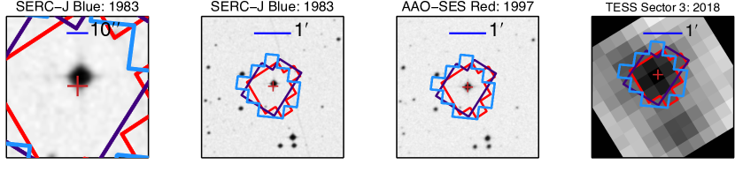
Supplementary Figure 1: Archival images and TESS image for TOI-270 from 1983 to 2018. The red plus shows the current position of TOI-270 in comparison. The regions mark the TESS aperture masks used in Sector 3 (red), 4 (purple) and 5 (blue). At the given spatial resolution, we see no background sources at the target’s current sky location.

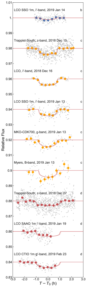
Supplementary Figure 2: Follow-up lightcurves for TOI-270 (see also Supplementary Table 1). Red lines show 20 lightcurves generated from randomly drawn posterior samples from the best-fit allesfitter model.

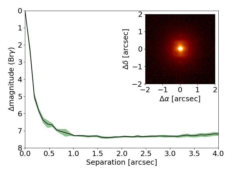
Supplementary Figure 3: Sensitivity of VLT/NaCo images to nearby companions, as a function of separation. Inset: 4” square image, centered on the target. No visual companions appear in this image, or anywhere within the field of view. Note that two point spread function artefacts appear 750 mas north and south of the host. These artefacts originate from the structure of the point spread function due to the target’s brightness, and are not visual companions.

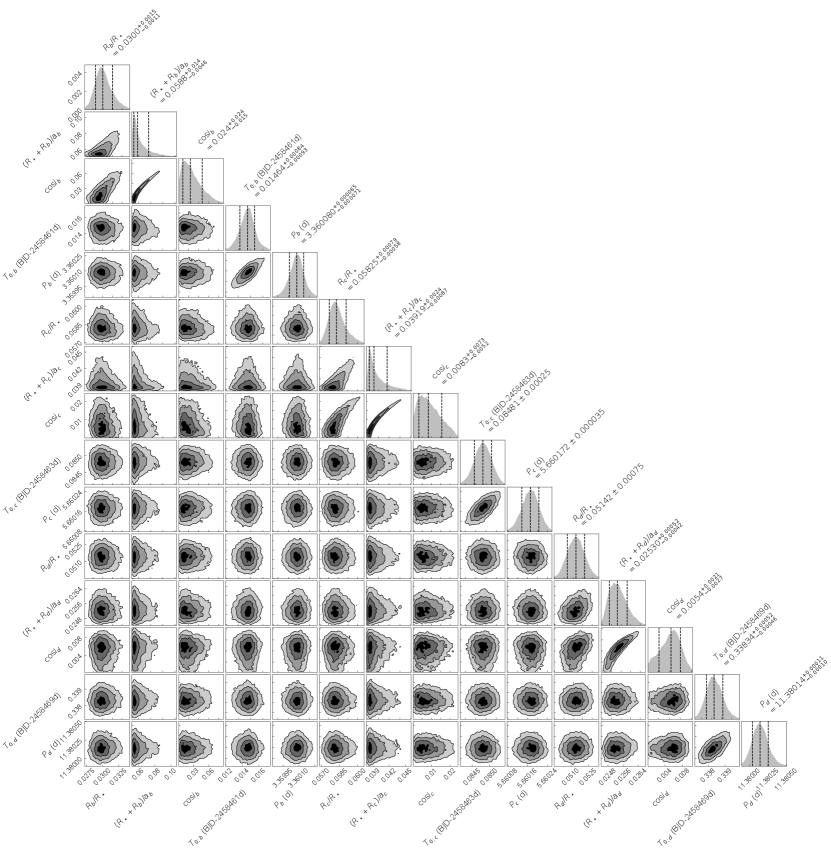
Supplementary Figure 4: Posterior probability distributions for all astrophysical parameters of the allesfitter nested sampling fit of TOI-270. The figure also highlights the correlation (or absence thereof) between all parameters. Vertical dashed lines show the median and 68% credible interval.

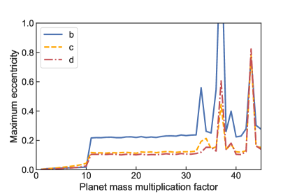
Supplementary Figure 5: Dynamical analysis based on the Mercury Integrator, showing the planets’ eccentricities over a range of masses (the predicted mass multiplied by a factor). The system is stable with eccentricities remaining below 0.05 for masses up to ten times the predicted mass. For masses 10–30 times higher, the system achieves stability but the interaction between planets begins to drive high eccentricities. At $\sim$30 times the original masses, the system would be chaotic.

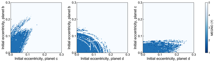
Supplementary Figure 6: Dynamical analysis based on MEGNO-maps. The configurations are as follow: Left, free eccentricities e_b and e_c in the range of 0 to 0.3, while e_d=0. Middle, free e_b and e_d, while e_c=0. Right, free e_c and e_d, while e_b=0. All other planetary parameters are fixed. In all cases: $\langle Y(t)\rangle\rightarrow 2$ for quasi-periodic orbits and $\langle Y(t)\rangle\rightarrow 5$ for chaotic systems. This shows that the system is stable for a range of low eccentricities.

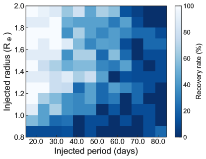
Supplementary Figure 7: A recovery test for injected transits of small planets in the terrestrial-like habitable zone of TOI-270 (corresponding to periods of 18–85 days). While larger transiting planets could have been found in the available TESS data, the regime of small exoplanets with period beyond $\sim$30 days remains open for future transit searches.

Supplementary Table 1: Observation Log

Discovery photometry
TOI-270	Dates	Telescope ${{\dagger}}$	Filter	Exposure	Nr. of	Duration	Transit	Aperture	FWHM
	(UTC)			time (sec)	exposures	(min)	coverage	radius (arcsec)	(arcsec)
b c d	2018-09-20	TESS	TESS	120	46874	–	–	30–60”	–
	– 2018-12-11
Follow-up photometry
TOI-270	Date	Telescope ${{\dagger}}$	Filter	Exposure	Nr. of	Duration	Transit	Aperture	FWHM	$\Delta\ln{Z}$§
	(UTC)			time (sec)	exposures	(min)	coverage	radius (arcsec)	(arcsec)
b	2018-12-18	PEST	Rc	120	189	449	Full	7.38	4.10	$<0$
	2018-12-25	LCO-CTIO	i′	20	113	113	Ingr.+$66\%$	7.78	4.30	$<0$
	2018-12-27	SS0-T17	Clear	60	120	151	Full	6.30	2.10	N/A‡
	2018-12-28	PEST	V	120	174	404	Full	7.38	4.00	$<0$
	2019-01-11	LCO-CTIO	i′	14	221	200	Full	8.94	2.10	$<0$
	2019-01-14	LCO-SSO	i′	15	178	161	Full	7.00	1.73	6.8§
	2019-01-24	LCO-SSO	g′	40	136	184	Full	4.23	2.14	$<0$
	2019-01-27	LCO-SAAO	g′	70	119	218	Full	7.78	2.28	$<0$
c	2018-12-15	TS	z′	10	698	242	Full	4.48	2.48	11.3§
	2018-12-16	LCO	i′	90	88	180	Full	5.83	–	19.2§
	2019-01-13	LCO-SSO	i′	11	207	216	Full	7.78	2.95	19.3§
	2019-01-13	PEST	V	120	143	335	Egr.+$90\%$	7.38	4.60	1.6
	2019-01-13	MKO	g′	128	82	247	Full	9.20	3.00	5.2§
	2019-01-13	Myers	B	180	70	300	Full	4.14	4.00	7.1§
d	2018-12-27	TS	z′	10	848	301	Full	4.48	2.31	4.3§
	2019-01-19	LCO-SAAO	i′	11	182	156	Ingr.+$77\%$	5.44	1.91	6.3§
	2019-02-23	LCO-CTIO	g′	70	123	203	Full	5.83	2.76	6.3§
Reconnaissance spectroscopy
TOI-270	Date	Telescope ${{\dagger}}$	Resolution	Wavelengths
	(UTC)
	2018-12-22	FIRE	6000	$8000-25000\,\text{\AA}$
	2019-01-23	ANU	23000	$3900-6700\,\text{\AA}$
High-resolution imaging
TOI-270	Date	Telescope ${{\dagger}}$	Filter	Exposure	Nr. of	FWHM
	(UTC)			time (sec)	exposures	(mas)
–	2019-01-25	NaCo	Ks	20	9	90

†Telescopes:
LCO-SSO: Las Cumbres Observatory - Siding Spring (1 m) [26]
LCO-CTIO: Las Cumbres Observatory - Cerro Tololo Interamerican Observatory (1 m) [26]
LCO-SAAO: Las Cumbres Observatory - South African Astronomical Observatory (1 m) [26]
TS: TRAPPIST-South (0.6 m) [27]
SSO-T17: Siding Spring Observatory - T17 (0.4 m)
PEST: The Perth Exoplanet Survey Telescope (0.3 m)
Myers: Myers-Siding Spring (0.4 m)
MKO: Mt. Kent Observatory CDK700 (0.7 m)
FIRE: Magellan Folded-port InfraRed Echellette (6.5 m) [28]
ANU: Australia National University Echelle spectrograph (2.3 m); spectrum reduced following [29]
NaCo: VLT NAOS-CONICA (8.2 m) [30, 31]
‡Observations not included, as deep exposures were used to study faint neighbouring stars and exclude possible blended eclipsing binaries.
§Only observations with a Bayes factor $\Delta\ln{Z}>3$ (strong evidence for a signal) are used for the global analysis.

Model	Free parameters	Bayes factor, $\Delta\ln{Z}$
circular, no TTVs	15	–
circular, free TTVs for all transits	57	<0
circular, free TTVs for planet b	33	2.4
circular, free TTVs for planet c	30	1.2
circular, free TTVs for planet d	24	<0
free eccentricity for all planets, no TTVs	21	<0
free eccentricity for planet b, no TTVs	17	2.6
free eccentricity for planet c, no TTVs	17	<0
free eccentricity for planet d, no TTVs	17	<0

Supplementary Table 2: A comparison of various models with different degrees of freedom. The Null Hypothesis, a circular model without TTVs, is compared against more complicated models allowing for free eccentricity and/or free TTVs. A Bayes factor >3 would mean strong Bayesian evidence for a model [32]. We thus find no strong Bayesian evidence for eccentricity nor TTVs.

Facility, date	$q_{1}$	$q_{2}$	$u_{1}$	$u_{2}$	$\ln{\sigma_{\mathrm{white}}}$	GP $\ln{\sigma}$	GP $\ln{\rho}$
TESS	$0.29_{-0.11}^{+0.20}$	$0.45_{-0.24}^{+0.26}$	$0.48_{-0.19}^{+0.16}$	$0.05_{--0.24}^{+0.34}$	$-6.6243_{-0.0034}^{+0.0032}$	$-8.712\pm 0.087$	$-1.97\pm 0.25$
LCO, 2018-12-16	$0.54\pm 0.28$	$0.18_{-0.12}^{+0.21}$	$0.26_{-0.16}^{+0.22}$	$0.45_{-0.36}^{+0.27}$	$-7.292\pm 0.079$	$-3.12_{-0.52}^{+0.73}$	$1.471\pm 0.045$
LCO CTIO, 2019-02-23	$0.62_{-0.26}^{+0.23}$	$0.64_{-0.29}^{+0.22}$	$0.93_{-0.45}^{+0.40}$	$-0.19\pm 0.68$	$-6.484\pm 0.067$	$-2.06\pm 0.55$	$0.981\pm 0.024$
LCO CTIO, 2018-12-25	$0.51\pm 0.31$	$0.51\pm 0.31$	$0.64_{-0.41}^{+0.53}$	$-0.01_{--0.24}^{+0.40}$	$-6.407_{-0.065}^{+0.070}$	$-10.5_{-2.8}^{+2.5}$	$0.3\pm 1.5$
LCO CTIO, 2019-01-11	$0.44_{-0.27}^{+0.31}$	$0.48\pm 0.30$	$0.55_{-0.35}^{+0.48}$	$0.02_{--0.18}^{+0.37}$	$-6.245\pm 0.048$	$-10.4_{-2.8}^{+3.5}$	$0.022\pm 0.038$
LCO SAAO, 2019-01-27	$0.57_{-0.31}^{+0.27}$	$0.54_{-0.31}^{+0.29}$	$0.72_{-0.45}^{+0.55}$	$-0.05_{--0.32}^{+0.42}$	$-6.472_{-0.064}^{+0.067}$	$-2.06\pm 0.54$	$1.100\pm 0.051$
LCO SAAO, 2019-01-19	$0.38_{-0.24}^{+0.31}$	$0.43_{-0.27}^{+0.31}$	$0.47_{-0.30}^{+0.40}$	$0.071_{--0.093}^{+0.37}$	$-5.833_{-0.051}^{+0.054}$	$-10.6_{-2.6}^{+2.5}$	$0.06\pm 0.11$
LCO SSO, 2019-01-24	$0.44_{-0.28}^{+0.33}$	$0.46_{-0.29}^{+0.32}$	$0.52_{-0.35}^{+0.51}$	$0.05_{--0.13}^{+0.37}$	$-6.011\pm 0.063$	$-2.19\pm 0.55$	$0.667\pm 0.063$
LCO SSO, 2019-01-13	$0.45_{-0.25}^{+0.29}$	$0.40_{-0.25}^{+0.31}$	$0.49_{-0.31}^{+0.38}$	$0.111_{--0.074}^{+0.37}$	$-5.937\pm 0.050$	$-11.0\pm 2.5$	$0.113\pm 0.086$
LCO SSO, 2019-01-14	$0.62_{-0.33}^{+0.25}$	$0.55_{-0.33}^{+0.28}$	$0.77_{-0.49}^{+0.57}$	$-0.07_{--0.35}^{+0.45}$	$-6.489\pm 0.056$	$-11.1\pm 2.4$	$0.037\pm 0.068$
MKO-CDK700, 2019-01-13	$0.59_{-0.31}^{+0.26}$	$0.53_{-0.30}^{+0.28}$	$0.74_{-0.44}^{+0.48}$	$-0.04_{--0.34}^{+0.42}$	$-6.112_{-0.081}^{+0.086}$	$-0.46_{-0.61}^{+0.55}$	$1.983\pm 0.020$
Myers, 2019-01-13	$0.52\pm 0.30$	$0.48\pm 0.31$	$0.61_{-0.40}^{+0.51}$	$0.02_{--0.19}^{+0.40}$	$-5.303_{-0.083}^{+0.088}$	$-10.2_{-2.9}^{+2.7}$	$2.00\pm 0.10$
PEST, 2018-12-18	$0.50\pm 0.30$	$0.50\pm 0.30$	$0.62_{-0.41}^{+0.53}$	$-0.00_{--0.22}^{+0.40}$	$-6.208_{-0.057}^{+0.061}$	$-2.18\pm 0.49$	$0.98\pm 0.16$
PEST, 2018-12-28	$0.48\pm 0.31$	$0.49\pm 0.30$	$0.59_{-0.39}^{+0.52}$	$0.01_{--0.20}^{+0.39}$	$-5.572\pm 0.054$	$-10.7_{-2.6}^{+2.4}$	$1.11\pm 0.15$
PEST, 2019-01-13	$0.48_{-0.29}^{+0.30}$	$0.50\pm 0.30$	$0.60_{-0.38}^{+0.51}$	$0.01_{--0.21}^{+0.39}$	$-5.445\pm 0.066$	$-7.8_{-4.3}^{+1.6}$	$1.36\pm 0.10$
Trappist-South, 2018-12-15	$0.26_{-0.17}^{+0.30}$	$0.38_{-0.24}^{+0.32}$	$0.35_{-0.22}^{+0.30}$	$0.101_{--0.027}^{+0.32}$	$-5.827\pm 0.027$	$-4.04\pm 0.33$	$-1.028\pm 0.035$
Trappist-South, 2018-12-27	$0.17_{-0.13}^{+0.28}$	$0.38_{-0.25}^{+0.33}$	$0.28_{-0.19}^{+0.30}$	$0.074_{--0.015}^{+0.29}$	$-5.604\pm 0.025$	$-3.82_{-0.63}^{+0.50}$	$-1.067\pm 0.037$

Supplementary Table 3: Nuisance parameters of the fit to individual observations, which are later fixed to their median values in the global analysis. These include the limb darkening parameters $q_{1}$ and $q_{2}$ in the parametrization suggested by [33] (for comparability also translated into the quadratic limb darkening parameters $u_{1}$ and $u_{2}$); the natural logarithm of the white noise scaling $\sigma_{\mathrm{white}}$; and the hyperparameters of the GP Matern-3/2, namely the natural logarithms of the amplitude $\sigma$ and characteristic time scale $\rho$.

TLS#	SNR	Depth	Period	First epoch	Note
		(mmag)	(d)	(BJDTDB)
1	85.8	3.9	5.65986	2458389.50438	planet c
2	54.1	3.1	11.38025	2458389.67737	planet d
3	21.1	0.9	3.36014	2458387.09273	planet b
4	8.3	0.2	5.53073	2458388.19620	shallow and too wide
5	6.5	0.6	13.90082	2458395.07980	falls in noisy regions$\dagger$

Supplementary Table 4: Threshold crossing events with a signal-to-noise ratio $\mathrm{SNR}\geq 5$ detected with transit least squares [34] in TESS Sectors 3–4 short-cadence data. The search is performed on the PDC-SAP lightcurves, which were additionally detrended using a Gaussian process. $\dagger$ Note that this signal might arise from systematics related to the satellite orbit ($\sim$13.7 days).

References

- [1] Fulton, B. J. & Petigura, E. A. The California-Kepler Survey. VII. Precise Planet Radii Leveraging Gaia DR2 Reveal the Stellar Mass Dependence of the Planet Radius Gap. Astron. J. 156, 264 (2018).
- [2] Van Eylen, V. et al. An asteroseismic view of the radius valley: stripped cores, not born rocky. Mon. Not. R. Astron. Soc. 479, 4786–4795 (2018).
- [3] Owen, J. E. & Wu, Y. Kepler Planets: A Tale of Evaporation. Astrophys. J. 775, 105 (2013).
- [4] Fortney, J. J., Marley, M. S. & Barnes, J. W. Planetary Radii across Five Orders of Magnitude in Mass and Stellar Insolation: Application to Transits. Astrophys. J. 659, 1661–1672 (2007).
- [5] Chen, J. & Kipping, D. Probabilistic Forecasting of the Masses and Radii of Other Worlds. Astrophys. J. 834, 17 (2017).
- [6] Deck, K. M., Agol, E., Holman, M. J. & Nesvorný, D. TTVFast: An Efficient and Accurate Code for Transit Timing Inversion Problems. Astrophys. J. 787, 132 (2014).
- [7] Crossfield, I. J. M. et al. A Nearby M Star with Three Transiting Super-Earths Discovered by K2. Astrophys. J. 804, 10 (2015).
- [8] Montet, B. T. et al. Stellar and Planetary Properties of K2 Campaign 1 Candidates and Validation of 17 Planets, Including a Planet Receiving Earth-like Insolation. Astrophys. J. 809, 25 (2015).
- [9] Dittmann, J. A. et al. A temperate rocky super-Earth transiting a nearby cool star. Nature 544, 333–336 (2017).
- [10] Lissauer, J. J. et al. Architecture and Dynamics of Kepler’s Candidate Multiple Transiting Planet Systems. Astrophys. J., Suppl. Ser. 197, 8 (2011).
- [11] Batalha, N. E. et al. PandExo: A Community Tool for Transiting Exoplanet Science with JWST and HST. Publ. Astron. Soc. Pacific 129, 064501 (2017).
- [12] Kempton, E. M. R. et al. A Framework for Prioritizing the TESS Planetary Candidates Most Amenable to Atmospheric Characterization. Publ. Astron. Soc. Pacific 130, 114401 (2018).
- [13] Hansen, B. M. S. & Murray, N. Testing in Situ Assembly with the Kepler Planet Candidate Sample. Astrophys. J. 775, 53 (2013).
- [14] Millholland, S., Wang, S. & Laughlin, G. Kepler Multi-planet Systems Exhibit Unexpected Intra-system Uniformity in Mass and Radius. Astrophys. J., Letters 849, L33 (2017).
- [15] Luger, R. & Barnes, R. Extreme Water Loss and Abiotic O2Buildup on Planets Throughout the Habitable Zones of M Dwarfs. Astrobiology 15, 119–143 (2015).
- [16] Serindag, D. B. & Snellen, I. A. G. Testing the Detectability of Extraterrestrial O2 with the Extremely Large Telescopes Using Real Data with Real Noise. Astrophys. J. 871, L7 (2019).
- [17] Schwieterman, E. W. et al. Identifying Planetary Biosignature Impostors: Spectral Features of CO and O4 Resulting from Abiotic O2/O3 Production. Astrophys. J. 819, L13 (2016). 1602.05584.
- [18] Takai, K. et al. Cell proliferation at 122°C and isotopically heavy CH4 production by a hyperthermophilic methanogen under high-pressure cultivation. Proc. Natl. Acad. Sci. 105, 10949–10954 (2008).
- [19] Noack, L. et al. Water-rich planets: How habitable is a water layer deeper than on Earth? Icarus 277, 215–236 (2016).
- [20] Kane, S. R. Worlds without Moons: Exomoon Constraints for Compact Planetary Systems. Astrophys. J. 839, L19 (2017).
- [21] Kopparapu, R. K. et al. Habitable Zones around Main-sequence Stars: Dependence on Planetary Mass. Astrophys. J. 787, L29 (2014).
- [22] Günther, M. N. et al. Stellar Flares from the First Tess Data Release: Exploring a New Sample of M-dwarfs. arXiv e-prints 1901.00443 (2019).
- [23] Newton, E. R., Irwin, J., Charbonneau, D., Berta-Thompson, Z. K. & Dittmann, J. A. The Impact of Stellar Rotation on the Detectability of Habitable Planets around M Dwarfs. Astrophys. J. 821, L19 (2016).
- [24] Lammer, H. et al. Coronal Mass Ejection (CME) Activity of Low Mass M Stars as An Important Factor for The Habitability of Terrestrial Exoplanets. II. CME-Induced Ion Pick Up of Earth-like Exoplanets in Close-In Habitable Zones. Astrobiology 7, 185–207 (2007).
- [25] Cohen, O. et al. The Interaction of Venus-like, M-dwarf Planets with the Stellar Wind of Their Host Star. Astrophys. J. 806, 41 (2015).
- [26] Tilley, M. A., Segura, A., Meadows, V., Hawley, S. & Davenport, J. Modeling Repeated M Dwarf Flaring at an Earth-like Planet in the Habitable Zone: Atmospheric Effects for an Unmagnetized Planet. Astrobiology 19, 64–86 (2019).
- [27] Gillon, M. et al. Seven temperate terrestrial planets around the nearby ultracool dwarf star TRAPPIST-1. Nature 542, 456–460 (2017).
- [28] Günther, M. N. & Daylan, T. allesfitter: Flexible star and exoplanet inference from photometry and radial velocity. Astrophysics Source Code Library (2019). ascl:1903.003.
- [29] Zeng, L., Sasselov, D. D. & Jacobsen, S. B. Mass-Radius Relation for Rocky Planets Based on PREM. Astrophys. J. 819, 127 (2016).
- [30] Stassun, K. G. & Torres, G. Evidence for a Systematic Offset of -80 as in the Gaia DR2 Parallaxes. Astrophys. J. 862, 61 (2018).

References

- [1] Stassun, K. G. et al. The TESS Input Catalog and Candidate Target List. Astron. J. 156, 102 (2018).
- [2] Muirhead, P. S. et al. A Catalog of Cool Dwarf Targets for the Transiting Exoplanet Survey Satellite. Astron. J. 155, 180 (2018).
- [3] Jenkins, J. M. The Impact of Solar-like Variability on the Detectability of Transiting Terrestrial Planets. Astrophys. J. 575, 493–505 (2002).
- [4] Jenkins, J. M. et al. Transiting planet search in the Kepler pipeline. In Software and Cyberinfrastructure for Astronomy, vol. 7740 of Proc. SPIE, 77400D (2010).
- [5] Smith, J. C. et al. Kepler Presearch Data Conditioning II - A Bayesian Approach to Systematic Error Correction. Publ. Astron. Soc. Pacific 124, 1000 (2012).
- [6] Stumpe, M. C. et al. Multiscale Systematic Error Correction via Wavelet-Based Bandsplitting in Kepler Data. Publ. Astron. Soc. Pacific 126, 100 (2014).
- [7] Jenkins, J. M. et al. The TESS science processing operations center. In Software and Cyberinfrastructure for Astronomy IV, vol. 9913 of Proc. SPIE, 99133E (2016).
- [8] Jenkins, J. M. Kepler Data Processing Handbook. Tech. Rep. (2017).
- [9] Cameron, A. C. Extrasolar planets: Astrophysical false positives. Nature 48–50.
- [10] Günther, M. N. et al. A new yield simulator for transiting planets and false positives: application to the Next Generation Transit Survey. Mon. Not. R. Astron. Soc. 465, 3379–3389 (2017).
- [11] Günther, M. N. et al. Unmasking the hidden NGTS-3Ab: a hot Jupiter in an unresolved binary system. Mon. Not. R. Astron. Soc. 478, 4720–4737 (2018).
- [12] Lissauer, J. J. et al. Almost All of Kepler’s Multiple-planet Candidates Are Planets. Astrophys. J. 750, 112 (2012).
- [13] Muirhead, P. S. et al. Characterizing the Cool KOIs. VI. H- and K-band Spectra of Kepler M Dwarf Planet-candidate Hosts. Astrophys. J., Suppl. Ser. 213, 5 (2014).
- [14] Gillon, M. et al. Temperate Earth-sized planets transiting a nearby ultracool dwarf star. Nature 533, 221–224 (2016).
- [15] Vanderspek, R. et al. TESS Discovery of an Ultra-short-period Planet around the Nearby M Dwarf LHS 3844. Astrophys. J. 871, L24 (2019).
- [16] Quinn, S. N. et al. Near-resonance in a system of sub-Neptunes from TESS. arXiv e-prints 1901.09092 (2019).
- [17] Twicken, J. D. et al. Kepler Data Validation I—Architecture, Diagnostic Tests, and Data Products for Vetting Transiting Planet Candidates. Publ. Astron. Soc. Pacific 130, 064502 (2018).
- [18] Li, J. et al. Kepler Data Validation II - Transit Model Fitting and Multiple-planet Search. Publ. Astron. Soc. Pacific 131, 024506 (2019).
- [19] Rizzuto, A. C. et al. Zodiacal Exoplanets in Time (ZEIT). VIII. A Two-planet System in Praesepe from K2 Campaign 16. Astron. J. 156, 195 (2018).
- [20] Winters, J. G. et al. The Solar Neighborhood. XXXV. Distances to 1404 m Dwarf Systems Within 25 pc in the Southern Sky. Astron. J. 149, 5 (2015).
- [21] Gaia Collaboration et al. Gaia Data Release 2. Summary of the contents and survey properties. Astron. Astrophys. 616, A1 (2018).
- [22] Winters, J. G. et al. The Solar Neighborhood. XLV. The Stellar Multiplicity Rate of M Dwarfs Within 25 pc. Astron. J. 157, 216 (2019).
- [23] Brown, T. M. et al. Las Cumbres Observatory Global Telescope Network. Publ. Astron. Soc. Pacific 125, 1031 (2013).
- [24] Jehin, E. et al. TRAPPIST: TRAnsiting Planets and PlanetesImals Small Telescope. The Messenger 145, 2–6 (2011).
- [25] Newton, E. R., Charbonneau, D., Irwin, J. & Mann, A. W. An Empirical Calibration to Estimate Cool Dwarf Fundamental Parameters from H-band Spectra. Astrophys. J. 800, 85 (2015).
- [26] Lenzen, R. et al. NAOS-CONICA first on sky results in a variety of observing modes. In Iye, M. & Moorwood, A. F. M. (eds.) Instrument Design and Performance for Optical/Infrared Ground-based Telescopes, vol. 4841 of Proc. SPIE, 944–952 (2003).
- [27] Rousset, G. et al. NAOS, the first AO system of the VLT: on-sky performance. In Wizinowich, P. L. & Bonaccini, D. (eds.) Adaptive Optical System Technologies II, vol. 4839 of Proc. SPIE, 140–149 (2003).
- [28] Morton, T. D. An Efficient Automated Validation Procedure for Exoplanet Transit Candidates. Astrophys. J. 761, 6 (2012).
- [29] Morton, T. D. VESPA: False positive probabilities calculator. Astrophysics Source Code Library (2015).
- [30] Stassun, K. G. & Torres, G. Evidence for a Systematic Offset of -80 as in the Gaia DR2 Parallaxes. Astrophys. J. 862, 61 (2018).
- [31] Jao, W.-C. et al. Distance-dependent Offsets between Parallaxes for Nearby Stars and Gaia DR1 Parallaxes. Astrophys. J., Letters 832, L18 (2016).
- [32] Benedict, G. F. et al. The Solar Neighborhood. XXXVII: The Mass-Luminosity Relation for Main-sequence M Dwarfs. Astron. J. 152, 141 (2016). 1608.04775.
- [33] Boyajian, T. S. et al. Stellar Diameters and Temperatures. II. Main-sequence K- and M-stars. Astrophys. J. 757, 112 (2012).
- [34] Mann, A. W. et al. How to Constrain Your M Dwarf. II. The Mass-Luminosity-Metallicity Relation from 0.075 to 0.70 Solar Masses. Astrophys. J. 871, 63 (2019).
- [35] Mann, A. W., Feiden, G. A., Gaidos, E., Boyajian, T. & von Braun, K. How to Constrain Your M Dwarf: Measuring Effective Temperature, Bolometric Luminosity, Mass, and Radius. Astrophys. J. 804, 64 (2015).
- [36] Pecaut, M. J. & Mamajek, E. E. Intrinsic Colors, Temperatures, and Bolometric Corrections of Pre-main-sequence Stars. Astrophys. J., Suppl. Ser. 208, 9 (2013).
- [37] Dittmann, J. A., Irwin, J. M., Charbonneau, D. & Newton, E. R. Calibration of the MEarth Photometric System: Optical Magnitudes and Photometric Metallicity Estimates for 1802 Nearby M-Dwarfs. Astrophys. J. 818, 153 (2016).
- [38] Mamajek, E. E. & Hillenbrand, L. A. Improved Age Estimation for Solar-Type Dwarfs Using Activity-Rotation Diagnostics. Astrophys. J. 687, 1264–1293 (2008).
- [39] Newton, E. R. et al. The Rotation and Galactic Kinematics of Mid M Dwarfs in the Solar Neighborhood. Astrophys. J. 821, 93 (2016).
- [40] Newton, E. R., Mondrik, N., Irwin, J., Winters, J. G. & Charbonneau, D. New Rotation Period Measurements for M Dwarfs in the Southern Hemisphere: An Abundance of Slowly Rotating, Fully Convective Stars. Astron. J. 156, 217 (2018).
- [41] Maxted, P. F. L. ellc: A fast, flexible light curve model for detached eclipsing binary stars and transiting exoplanets. Astron. Astrophys. 591, A111 (2016).
- [42] Davenport, J. R. A. et al. Kepler Flares. II. The Temporal Morphology of White-light Flares on GJ 1243. Astrophys. J. 797, 122 (2014).
- [43] Speagle, J. S. dynesty: A Dynamic Nested Sampling Package for Estimating Bayesian Posteriors and Evidences. arXiv e-prints 1904.02180 (2019).
- [44] Foreman-Mackey, D., Hogg, D. W., Lang, D. & Goodman, J. emcee: The MCMC Hammer. Publ. Astron. Soc. Pacific 125, 306 (2013). ascl:1202.3665.
- [45] Foreman-Mackey, D., Agol, E., Ambikasaran, S. & Angus, R. celerite: Scalable 1D Gaussian Processes in C++, Python, and Julia. Astrophysics Source Code Library (2017). ascl:1709.008.
- [46] Kass, R. E. & Raftery, A. E. Bayes factors. Journal of the American Statistical Association 90, 773–795 (1995).
- [47] Seager, S. & Mallén-Ornelas, G. A Unique Solution of Planet and Star Parameters from an Extrasolar Planet Transit Light Curve. Astrophys. J. 585, 1038–1055 (2003).
- [48] Eastman, J. EXOFASTv2: Generalized publication-quality exoplanet modeling code. Astrophysics Source Code Library (2017). ascl:1710.003.
- [49] Hippke, M. & Heller, R. Optimized transit detection algorithm to search for periodic transits of small planets. Astron. Astrophys. 623, A39 (2019).
- [50] Kovács, G., Zucker, S. & Mazeh, T. A box-fitting algorithm in the search for periodic transits. Astron. Astrophys. 391, 369–377 (2002).
- [51] Mandel, K. & Agol, E. Analytic light curves for planetary transit searches. The Astrophysical Journal Letters 580, L171.
- [52] Kreidberg, L. batman: BAsic Transit Model cAlculatioN in Python. Publ. Astron. Soc. Pacific 127, 1161 (2015).
- [53] Ricker, G. R. et al. Transiting Exoplanet Survey Satellite (TESS). In Proc. SPIE, vol. 9143, 20 (2014).
- [54] Simcoe, R. A. et al. FIRE: A Facility Class Near-Infrared Echelle Spectrometer for the Magellan Telescopes. Publ. Astron. Soc. Pacific 125, 270 (2013).
- [55] Skrutskie, M. F. et al. The Two Micron All Sky Survey (2MASS). Astron. J. 131, 1163–1183 (2006).
- [56] Gaia Collaboration et al. The Gaia mission. Astron. Astrophys. 595, A1 (2016). 1609.04153.
- [57] Zacharias, N. et al. The Fourth US Naval Observatory CCD Astrograph Catalog (UCAC4). Astron. J. 145, 44 (2013).
- [58] van Rossum, G. Python tutorial. Tech. Rep. CS-R9526, Centrum voor Wiskunde en Informatica (CWI), Amsterdam (1995).
- [59] van der Walt, S., Colbert, S. C. & Varoquaux, G. The numpy array: A structure for efficient numerical computation. Computing in Science & Engineering 13, 22–30 (2011). URL http://aip.scitation.org/doi/abs/10.1109/MCSE.2011.37. http://aip.scitation.org/doi/pdf/10.1109/MCSE.2011.37.
- [60] Jones, E., Oliphant, T., Peterson, P. et al. SciPy: Open source scientific tools for Python (2001). URL http://www.scipy.org/.
- [61] Hunter, J. D. Matplotlib: A 2d graphics environment. Computing in Science & Engineering 9, 90–95 (2007). URL http://aip.scitation.org/doi/abs/10.1109/MCSE.2007.55. http://aip.scitation.org/doi/pdf/10.1109/MCSE.2007.55.
- [62] Foreman-Mackey, D. corner.py: Scatterplot matrices in python. The Journal of Open Source Software 24 (2016). URL http://dx.doi.org/10.5281/zenodo.45906.
- [63] Jensen, E. Tapir: A web interface for transit/eclipse observability. Astrophysics Source Code Library (2013). ascl:1306.007.
- [64] Collins, K. A., Kielkopf, J. F., Stassun, K. G. & Hessman, F. V. AstroImageJ: Image Processing and Photometric Extraction for Ultra-precise Astronomical Light Curves. Astron. J. 153, 77 (2017).
- [65] Rein, H. & Liu, S.-F. REBOUND: an open-source multi-purpose N-body code for collisional dynamics. Astron. Astrophys. 537, A128 (2012).

References

- [1] Skilling, J. Nested Sampling. In Fischer, R., Preuss, R. & Toussaint, U. V. (eds.) American Institute of Physics Conference Series, vol. 735, 395–405 (2004).
- [2] Hall, R. D., Thompson, S. J., Handley, W. & Queloz, D. On the Feasibility of Intense Radial Velocity Surveys for Earth-Twin Discoveries. Mon. Not. R. Astron. Soc. 479, 2968–2987 (2018). 1806.00518.
- [3] Foreman-Mackey, D., Agol, E., Ambikasaran, S. & Angus, R. celerite: Scalable 1D Gaussian Processes in C++, Python, and Julia. Astrophysics Source Code Library (2017). ascl:1709.008.
- [4] Chambers, J. E. A hybrid symplectic integrator that permits close encounters betw een massive bodies. Mon. Not. R. Astron. Soc. 304, 793–799 (1999).
- [5] Duncan, M. J., Levison, H. F. & Lee, M. H. A Multiple Time Step Symplectic Algorithm for Integrating Close E ncounters. Astron. J. 116, 2067–2077 (1998).
- [6] Kane, S. R. Stability of Earth-mass Planets in the Kepler-68 System. Astrophys. J., Letters 814, L9 (2015). 1511.02882.
- [7] Kane, S. R. Resolving Close Encounters: Stability in the HD 5319 and HD 7924 Planetary Systems. Astrophys. J. 830, 105 (2016). 1608.02590.
- [8] Cincotta, P. & Simó, C. Conditional Entropy. Celestial Mechanics and Dynamical Astronomy 73, 195–209 (1999).
- [9] Cincotta, P. M. & Simó, C. Simple tools to study global dynamics in non-axisymmetric galactic potentials - I. Astronomy and Astrophysics Supplement Series 147, 205–228 (2000).
- [10] Cincotta, P. M., Giordano, C. M. & Simó, C. Phase space structure of multi-dimensional systems by means of the mean exponential growth factor of nearby orbits. Physica D Nonlinear Phenomena 182, 151–178 (2003).
- [11] Rein, H. & Liu, S.-F. REBOUND: an open-source multi-purpose N-body code for collisional dynamics. Astron. Astrophys. 537, A128 (2012).
- [12] Rein, H. & Tamayo, D. WHFAST: a fast and unbiased implementation of a symplectic Wisdom-Holman integrator for long-term gravitational simulations. Mon. Not. R. Astron. Soc. 452, 376–388 (2015). 1506.01084.
- [13] Alexander, M. E. The Weak Friction Approximation and Tidal Evolution in Close Binary Systems. Astrophysics and Space Science 23, 459–510 (1973).
- [14] Mignard, F. The Evolution of the Lunar Orbit Revisited. I. Moon and Planets 20, 301–315 (1979).
- [15] Hut, P. Tidal evolution in close binary systems. Astron. Astrophys. 99, 126–140 (1981).
- [16] Eggleton, P. P., Kiseleva, L. G. & Hut, P. The Equilibrium Tide Model for Tidal Friction. Astrophys. J. 499, 853–870 (1998). astro-ph/9801246.
- [17] Leconte, J., Chabrier, G., Baraffe, I. & Levrard, B. Is tidal heating sufficient to explain bloated exoplanets? Consistent calculations accounting for finite initial eccentricity. Astron. Astrophys. 516, A64 (2010). 1004.0463.
- [18] Bolmont, E., Raymond, S. N., Leconte, J., Hersant, F. & Correia, A. C. M. Mercury-T: A new code to study tidally evolving multi-planet systems. Applications to Kepler-62. Astron. Astrophys. 583, A116 (2015). 1507.04751.
- [19] Blanco-Cuaresma, S. & Bolmont, E. What can the programming language Rust do for astrophysics? In Brescia, M., Djorgovski, S. G., Feigelson, E. D., Longo, G. & Cavuoti, S. (eds.) Astroinformatics, vol. 325 of IAU Symposium, 341–344 (2017). 1702.02951.
- [20] Neron de Surgy, O. & Laskar, J. On the long term evolution of the spin of the Earth. Astron. Astrophys. 318, 975–989 (1997).
- [21] Fortney, J. J., Marley, M. S. & Barnes, J. W. Planetary Radii across Five Orders of Magnitude in Mass and Stellar Insolation: Application to Transits. Astrophys. J. 659, 1661–1672 (2007).
- [22] Chen, J. & Kipping, D. Probabilistic Forecasting of the Masses and Radii of Other Worlds. Astrophys. J. 834, 17 (2017).
- [23] McCarthy, C. & Castillo-Rogez, J. Planetary Ices Attenuation Properties, vol. 183 (2013).
- [24] Kopparapu, R. K. et al. Habitable Zones around Main-sequence Stars: New Estimates. Astrophys. J. 765, 131 (2013).
- [25] Kopparapu, R. K. et al. Habitable Zones around Main-sequence Stars: Dependence on Planetary Mass. Astrophys. J. 787, L29 (2014).
- [26] Brown, T. M. et al. Las Cumbres Observatory Global Telescope Network. Publ. Astron. Soc. Pacific 125, 1031 (2013).
- [27] Jehin, E. et al. TRAPPIST: TRAnsiting Planets and PlanetesImals Small Telescope. The Messenger 145, 2–6 (2011).
- [28] Simcoe, R. A. et al. FIRE: A Facility Class Near-Infrared Echelle Spectrometer for the Magellan Telescopes. Publ. Astron. Soc. Pacific 125, 270 (2013).
- [29] Zhou, G. et al. The mass-radius relationship for very low mass stars: four new discoveries from the HATSouth Survey. Mon. Not. R. Astron. Soc. 437, 2831–2844 (2014). 1310.7591.
- [30] Lenzen, R. et al. NAOS-CONICA first on sky results in a variety of observing modes. In Iye, M. & Moorwood, A. F. M. (eds.) Instrument Design and Performance for Optical/Infrared Ground-based Telescopes, vol. 4841 of Proc. SPIE, 944–952 (2003).
- [31] Rousset, G. et al. NAOS, the first AO system of the VLT: on-sky performance. In Wizinowich, P. L. & Bonaccini, D. (eds.) Adaptive Optical System Technologies II, vol. 4839 of Proc. SPIE, 140–149 (2003).
- [32] Kass, R. E. & Raftery, A. E. Bayes factors. Journal of the American Statistical Association 90, 773–795 (1995).
- [33] Kipping, D. M. Efficient, uninformative sampling of limb darkening coefficients for two-parameter laws. Mon. Not. R. Astron. Soc. 435, 2152–2160 (2013). 1308.0009.
- [34] Hippke, M. & Heller, R. Optimized transit detection algorithm to search for periodic transits of small planets. Astron. Astrophys. 623, A39 (2019).