Efficient, uninformative sampling of limb darkening coefficients for two-parameter lawsEfficient, uninformative sampling of limb darkening coefficients for two-parameter laws–References2013

Abstract

Stellar limb darkening affects a wide range of astronomical measurements and is frequently modelled with a parametric model using polynomials in the cosine of the angle between the line of sight and the emergent intensity. Two-parameter laws are particularly popular for cases where one wishes to fit freely for the limb darkening coefficients (i.e. an uninformative prior) due to the compact prior volume and the fact that more complex models rarely obtain unique solutions with present data. In such cases, we show that the two limb darkening coefficients are constrained by three physical boundary conditions, describing a triangular region in the two-dimensional parameter space. We show that uniformly distributed samples may be drawn from this region with optimal efficiency by a technique developed by computer graphical programming: triangular sampling. Alternatively, one can make draws using a uniform, bivariate Dirichlet distribution. We provide simple expressions for these parametrizations for both techniques applied to the case of quadratic, square-root and logarithmic limb darkening laws. For example, in the case of the popular quadratic law, we advocate fitting for $q_{1}\equiv(u_{1}+u_{2})^{2}$ and $q_{2}\equiv 0.5u_{1}(u_{1}+u_{2})^{-1}$ with uniform priors in the interval $[0,1]$ to implement triangular sampling easily. Employing these parametrizations allows one to derive model parameters which fully account for our ignorance about the intensity profile, yet never explore unphysical solutions, yielding robust and realistic uncertainty estimates. Furthermore, in the case of triangular sampling with the quadratic law, our parametrization leads to significantly reduced mutual correlations and provides an alternative geometric explanation as to why naively fitting the quadratic limb darkening coefficients precipitates strong correlations in the first place.

1 Introduction

Stellar limb darkening is the wavelength-dependent diminishing of the surface brightness from the centre of the disc to the limb of the star. Limb darkening affects a wide range of different astronomical observations, such as optical interferometry (e.g. Aufdenberg et al. 2005), microlensing light curves (e.g. Witt 1995; Zub et al. 2011), rotational modulations (Kipping 2012), eclipsing binaries (Kopal 1950) and transiting planets (Mandel & Agol 2002). Due to the often subtle, profile distorting effects of limb darkening, the parameters describing limb darkening are frequently degenerate with other model parameters of interest, and thus accurate modelling is crucial in the interpretation of such data.

Many of these astronomical phenomena may be described with precise closed-form analytic solutions, if one assumes a parametric limb darkening law. For example, the transit light curve may be expressed using hypergeometric functions and elliptical integrals when one adopts a polynomial law (Mandel & Agol 2002; Kjurkchieva et al. 2013). Such closed forms are not only computationally expedient to evaluate, but their parametrization also easily allows for uninformative priors on a target star’s properties and Bayesian model selection of different laws, since the prior volume can be directly controlled.

Many of the commonly employed parametric limb darkening laws have been chosen to provide the best approximation possible between stellar atmosphere model intensity profiles and simple polynomial expansions (e.g. Claret 2000; Claret & Hauschildt 2003; Sing 2010; Hayek et al. 2012). This is because a typical approach was to regress a model to some observations whilst assuming a fixed stellar limb darkening law which most realistically described the modeller’s expectation for the star. The benefits of this approach are that the parameters describing the limb darkening do not have to be varied, making the regressions considerably easier. However, an obvious consequence of this is that any model parameters derived from such an approach are fundamentally dependent upon the stellar atmosphere model adopted. An equivalent way of describing this approach is that a Dirac delta function prior was adopted for the limb darkening profile, which is statistically an implausible scenario.

An alternative strategy is to relax the constraint to weaker or even uninformative priors. However, the trade-off is that by adopting a finite prior volume for the parameters describing the limb darkening, it is strongly preferred to use as compact a parametric model as possible (i.e. fewer parameters) so that the regression algorithm can reasonably hope to explore the full parameter space. Nevertheless, this is a statistically more robust approach than simply fixing these parameters, which are frequently correlated to the other model terms (Pal 2008).

An example of a weaker prior would be to regress a joint probability density function (PDF) to the limb darkening coefficients (LDCs) emerging from an ensemble of stellar atmosphere models (e.g. Kipping et al. 2013). However, even this approach is still fundamentally dependent upon stellar atmosphere models, since it is from these models that the ensemble of coefficients is initially computed. In contrast, uninformative priors make no assumption about the limb darkening profile, except for the parametric form which describes the intensity profile (e.g. the polynomial orders used). Such an approach may even be used to reverse engineer properties of individual stars or populations thereof (Neilson & Lester 2012), although Howarth 2011 cautions that one must carefully account for the system geometry when comparing fitted LDCs and those from stellar atmosphere models.

Adopting a simple parametric limb darkening law with uninformative priors is therefore a powerful way of (i) incorporating and propagating our ignorance about the target star’s true intensity profile into the derivation of all model parameters, (ii) presenting results which are independent of theoretical stellar atmosphere models, (iii) modelling astronomical phenomenon using closed-form and thus highly expedient algorithms and (iv) providing insights and constraints on the fundamental properties of the target star.

The most common choice of uninformative prior for LDCs is a simple uniform prior. One danger of uninformative priors is that allowing the LDCs to explore any parameter range can often lead to unphysical limb darkening profiles being explored. It is therefore necessary to impose boundary conditions which prevent such violations. In this work, we show that after imposing the said boundary conditions (§2.1), the PDF describing an uninformative joint prior on the quadratic LDCs is a uniform, bivariate Dirichlet distribution (§2.4). Furthermore, we show that one may efficiently sample from this distribution using a trick from the field of computer graphical programming: triangular sampling (§2.5). This results in a new parametrization for the quadratic LDCs which samples the physically plausible range of LDCs in an optimally efficient and complete manner. By comparing our results to previously proposed parametrizations, we show that this approach is at least twice as efficient as all others (§3). Finally, we provide optimal parametrizations using triangular sampling for other two-parameter limb darkening laws (§4).

2 Quadratic Limb Darkening Law

2.1 Deriving the three boundary conditions

We begin by considering the quadratic limb darkening law due its wide ranging use in a variety of fields. We first derive the boundary conditions which constrain the physically plausible range of the associated LDCs. Note, this is not the first presentation of such constraints (e.g. Burke et al. 2007), but due to some distinct constraints present elsewhere in the literature (e.g. Carter et al. 2009) and the fact that this derivation serves as a template for the applying constraints to other two-parameter limb darkening laws (e.g. see later §4), we present an explicit derivation here.

We begin by considering the widely used quadratic limb darkening law. The quadratic law seems to have first appeared in Kopal 1950 and is attractive due to its simple, intuitive form, flexibility to explore a range of profiles plus a fairly compact, efficient structure. The specific intensity of a star, $I(\mu)$, following the quadratic limb darkening may be described by

$$I(\mu)/I(1) =1-u_{1}(1-\mu)-u_{2}(1-\mu)^{2},$$ (1)

where $I(1)$ is the specific intensity at the centre of the disc, $u_{1}$ and $u_{2}$ are the quadratic LDCs and $\mu$ is the cosine of the angle between the line of sight and the emergent intensity. We may also express $\mu=\sqrt{1-r^{2}}$, where $r$ is the normalized radial coordinate on the disc of the star.

We wish to investigate whether imposing some physical conditions on this expression leads to any useful constraints on the allowed ranges of the coefficients $u_{1}$ and $u_{2}$. In what follows, we define physically plausible limb darkening profiles in reference to broad bandpass photometric/imaging observations of normal main-sequence stars (i.e. we do not consider pulsars, white dwarfs, brown dwarfs, etc). Accordingly, we may impose the following two physical conditions:

• an everywhere-positive intensity profile,

• a monotonically decreasing intensity profile from the centre of the star to the limb.

Condition (A) requires little justification since a negative intensity has no physical meaning and it may be expressed algebraically as $I(\mu)>0$ $\forall$ $0\leq\mu<1$, or

$$u_{1}(1-\mu)+u_{2}(1-\mu)^{2}<1\,\,\,\,\,\forall\,\,\,\,\,\,0\leq\mu<1.$$ (2)

The above can be evaluated in one of two extrema; minimizing the LHS with respect to $\mu$ and maximizing the LHS with respect to $\mu$. Consider first minimizing the LHS, which is trivially found to occur for $\mu\rightarrow 1$. This leaves us with the meaningless constraint that $0<1$, which is of course satisfied for all $u_{1}$ and $u_{2}$ and thus leads to no useful constraints on the LDCs.

The other extrema of this condition is found by evaluating the LHS at its maximum, which is again trivially found to occur when $\mu\rightarrow 0$ and leads us to

$$u_{1}+u_{2}<1.$$ (3)

Therefore, the physical requirement of an everywhere-positive intensity profile leads to a single constraint on the LDCs, given by equation (3).

Next, let us enforce condition (B), that the specific intensity is a monotonically decreasing function towards the limb. This is generally expected for any broad bandpass limb darkening profile (Burke et al. 2007), but some narrow spectral lines, such as Si IV, could produce limb-brightened profiles (Schlawin et al. 2010). Focusing on the much more common case of limb darkening though, we have

$$\frac{\partial I(\mu)}{\partial\mu}>0,$$ (4)

which is easily shown to give

$$u_{1}+2u_{2}(1-\mu)>0.$$ (5)

One of the extrema of this condition is found by minimizing the LHS with respect to $\mu$, which occurs for $\mu\rightarrow 1$, giving

$$u_{1}>0.$$ (6)

The other extrema occurs when we maximize the LHS with respect to $\mu$, which occurs for $\mu\rightarrow 0$ and gives

$$u_{1}+2u_{2}>0.$$ (7)

We therefore derive two constraints on the LDCs from condition (B) (equations 6 & 7). In total then, we have three boundary conditions on the coefficients $u_{1}$ and $u_{2}$:

$$u_{1}+u_{2} <1,$$

$$u_{1} >0,$$

$$u_{1}+2u_{2} >0.$$ (8)

2.2 Comparison to previous works

Before proceeding to our new parametrization model, we pause to compare our derived boundary conditions to those in previous works. The first explicit declaration of a set of expressions used to enforce physically plausible LDCs, that we are aware of, seems to come from Burke et al. 2007. Here, the authors state all three of the same boundary conditions (see §3.2 of that work) stated here in equation (8). This is not surprising as Burke et al. 2007 enforced the same physical criteria [i.e. conditions (A) and (B)] to derive their expressions, i.e. an everywhere-positive intensity profile and a monotonically decreasing brightness from the centre-to-limb.

Another paper stating boundary conditions on the LDCs comes from Carter et al. 2009, where the authors used the conditions $(u_{1}+u_{2})<1$, $u_{1}>0$ and $(u_{1}+u_{2})>0$. We point out that the last constraint seems to be a typographical error missing a ‘2’, but otherwise are the same as those constraints provided here. We highlight this minor point to avoid potential confusion in comparing these works.

2.3 Visualizing the constraints

In order to visualize the constraints of equation (8), we generated $u_{1}$ and $u_{2}$ by naively randomly sampling a uniform distribution bounded by $-3<u_{1}<+3$ and $-3<u_{2}<+3$. For every realization, we only accept the draw if all of the constraints in equation (8) are satisfied, as shown in Fig. 1. Iterating until $10^{5}$ trials were accepted, we required 3.6 million trials, i.e. an efficiency of 2.8%. This highlights how inefficient it would be to sample from such a joint distribution.

Figure 1: Drawing $u_{1}$ and $u_{2}$ from a uniform distribution between $-3$ and $+3$, we show the realizations which satisfy the physical constraints of equation (8). The black dashed lines describe the three constraints. The loci of accepted points form a triangle with a bisector inclined $35.8^{\circ}$ to the $u_{1}$-axis.

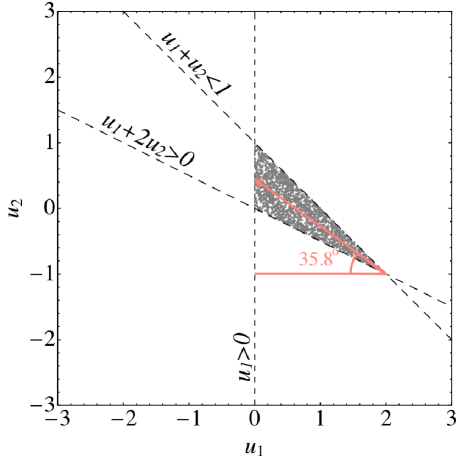
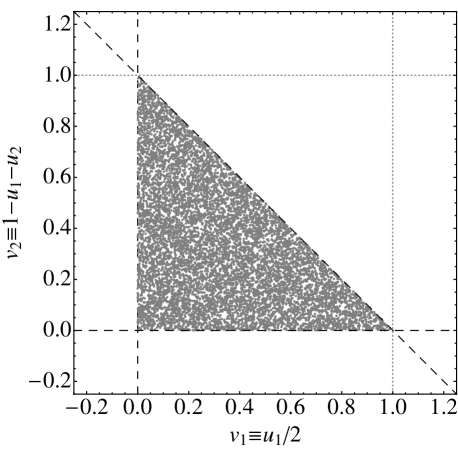
One may re-plot Fig. 1 using different axes to visualize the constraints in alternative ways. We found that one particularly useful way of visualizing the constraints was found by plotting $v_{1}$ against $v_{2}$, as shown in Fig. 2, where we use the parametrization:

$$v_{1} \equiv u_{1}/2,$$ (9)

$$v_{2} \equiv 1-u_{1}-u_{2}.$$ (10)

Using this parametrization, Fig. 2 reveals the loci of points satisfying conditions (A) and (B) form a right-angled triangle.

Figure 2: Same as Fig. 1, except that we have re-parametrized the two axes. One can see that the allowed physical range falls within a triangle which covers exactly one half of the unit square $\{0,0\}\rightarrow\{0,1\}\rightarrow\{1,1\}\rightarrow\{1,0\}$. This square describes the constraints stated in Carter et al. 2009, which violate condition (B).

2.4 Physical priors using the Dirichlet distribution

For those familiar with the Dirichlet distribution, the shape of Fig. 2 will bear an uncanny resemblance to the uniform, bivariate Dirichlet distribution. The Dirichlet distribution is a multivariate generalization of the Beta distribution (which itself has useful applications as a prior; Kipping 2013). Aside from being able to exactly reproduce the distribution shown in Fig. 2, the bivariate Dirichlet distribution is able to reproduce a diverse range of profiles with just three so-called ‘concentration’ parameters ($\mn@boldsymbol{\alpha}=\{\alpha_{1},\alpha_{2},\alpha_{3}\}^{T}$). The PDF is given by

$$\mathrm{P}(\mn@boldsymbol{\alpha};v_{1},v_{2}) =\frac{v_{1}^{\alpha_{2}-1}v_{2}^{\alpha_{1}-1}(1-v_{1}-v_{2})^{\alpha_{3}-1}\Gamma[\alpha_{1}+\alpha_{2}+\alpha_{3}]}{\Gamma[\alpha_{1}]\Gamma[\alpha_{2}]\Gamma[\alpha_{3}]},$$ (11)

for $v_{1}>0$, $v_{2}>0$ and $(v_{1}+v_{2})<1$; otherwise $\mathrm{P}(\mn@boldsymbol{\alpha};v_{1},v_{2})=0$. In the case of the uniform distribution of Fig. 2, one may simply use $\mn@boldsymbol{\alpha}=\mathbf{1}$:

$$\mathrm{P}(\mn@boldsymbol{\alpha}=\mathbf{1};v_{1},v_{2})=\begin{cases}2&\text{if}\ v_{1}>0\ \mathrm{\&}\ v_{2}>0\ \mathrm{\&}\ (v_{1}+v_{2})<1,\\ 0&\text{otherwise}.\end{cases}$$

The bivariate Dirichlet distribution is also uniquely defined over the range $v_{1}>0$, $v_{2}>0$ and $(v_{1}+v_{2})<1$ and naturally integrates to unity over this range. It may therefore be used to serve as a proper prior.

2.5 Physical priors using triangular sampling

Consider the special case where one requires sampling from a uniform prior in the joint distribution $\{u_{1},u_{2}\}$ (but wishes to enforce that all sampled realizations are physical). This corresponds to the uniform, bivariate Dirichlet distribution described by equation (11) with $\mn@boldsymbol{\alpha}=\mathbf{0}$. One therefore needs to simply draw a random variate in $\{v_{1},v_{2}\}$ from the uniform, bivariate Dirichlet distribution.

However, another way of thinking about the problem is to try to populate a triangle with a uniform sampling of points, as evident from Fig. 2 - a procedure we dub ‘triangular sampling’. This more geometric perspective leads to a simple and elegant expression for generating the LDC samples.

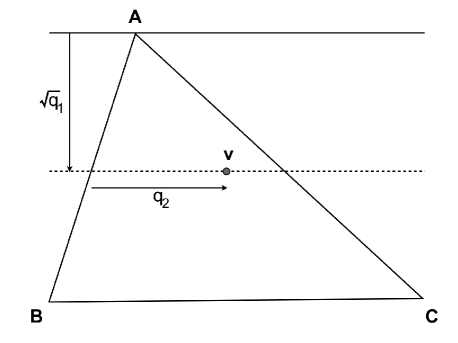
An elegant method for triangular sampling comes from the field of computer graphical programming, which we will describe here. Consider a triangle with vertices $\mathbf{A}$, $\mathbf{B}$ and $\mathbf{C}$, and two random uniform variates $q_{1}$ and $q_{2}$ in the interval $[0,1]$. Turk 1990 showed that a random location, $\mathbf{v}$, within the triangle can be sampled using (notation has been changed slightly from that of Turk 1990)

$$\mathbf{v} =(1-\sqrt{q_{1}})\mathbf{A}+\sqrt{q_{1}}(1-q_{2})\mathbf{B}+q_{2}\sqrt{q_{1}}\mathbf{C}.$$ (12)

This sampling is equivalent to having $q_{1}$ draw out a line segment parallel to $BC$ that joins a point on $AB$ with a point on $AC$ and then selecting a point on this segment based upon the value of $q_{2}$ (as shown in Fig. 3). Taking the square root of $q_{1}$ is necessary to weight all portions of the triangle equally.

Figure 3: A geometric illustration of how a random point is drawn from a triangle with vertices $A$, $B$ and $C$ using two random variates $q_{1}$ and $q_{2}$ (i.e. ‘triangular sampling’). The method and figure adapted are from the computer graphical programming chapter of Turk 1990.

Evaluating the above for $\mathbf{A}=\{0,1\}^{T}$, $\mathbf{B}=\{0,0\}^{T}$ and $\mathbf{C}=\{1,0\}^{T}$ (representing the vertices of the specific triangle we are interested in) gives

$$v_{1} =\sqrt{q_{1}}q_{2},$$ (13)

$$v_{2} =1-\sqrt{q_{1}}.$$ (14)

Substituting the above into equations (9) and (10) gives

$$u_{1} =2\sqrt{q_{1}}q_{2},$$ (15)

$$u_{2} =\sqrt{q_{1}}(1-2q_{2}).$$ (16)

The inverse of these expressions are easily found to be given by

$$q_{1} \equiv(u_{1}+u_{2})^{2},$$ (17)

$$q_{2} \equiv\frac{u_{1}}{2(u_{1}+u_{2})}.$$ (18)

By re-parametrizing the LDCs from a set $\mn@boldsymbol{\theta}$ of $\mn@boldsymbol{\theta}=\{u_{1},u_{2}\}$ to $\mn@boldsymbol{\theta}=\{q_{1},q_{2}\}$, one can fit for quadratic LDCs in such a way that the joint prior distribution is uniform and exclusively samples physically plausible solutions. For example, one would fit for $q_{1}$ and $q_{2}$ with uniform priors between $0$ and $1$, but convert these parameters into $u_{1}$ and $u_{2}$ (using equation 15 & 16) before calling their light curve generation code e.g. the Mandel & Agol 2002 algorithm. This will exactly reproduce the uniform, bivariate Dirichlet distribution shown in Fig. 1 & 2.

2.6 Comparison to theoretical stellar atmosphere models

By sampling from $\mn@boldsymbol{\theta}=\{q_{1},q_{2}\}$ uniformly over the interval $[0,1]$, one adopts uninformative priors in the LDCs and thus the underlying intensity profile of a given star. The only physics which goes into our model are the conditions (A) and (B). In contrast, LDCs generated using stellar atmosphere models include a great deal of physics, and sampling coefficients from such a model is more appropriately described as using informative priors. The choice as to which path to follow is a matter for the data analyst to decide and is likely dependent upon how well characterized the target star is and how much trust is placed in the theoretical models.

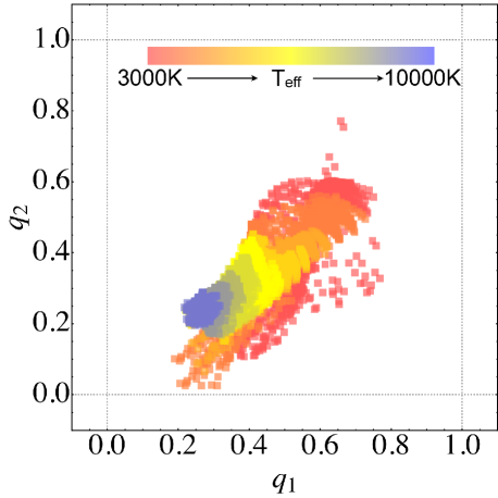
An implicit expectation of our $\mn@boldsymbol{\theta}=\{q_{1},q_{2}\}$ model is that the true LDCs of normal stars observed in a broad bandpass should fall within the unit-square of $0<q_{1}<1$ and $0<q_{2}<1$. By extension then, the LDCs of a realistic stellar atmosphere should also reproduce coefficients lying within this unit-square. To check this, we here show the results of converting standard tabulations of quadratic LDCs into the $\mn@boldsymbol{\theta}=\{q_{1},q_{2}\}$ parametrization. We decide to use the Kepler bandpass for this comparison since our model is (a) designed for broad bandpass photometry, (b) most useful for faint target stars with poor characterization requiring uninformative priors and (c) likely to be most commonly employed on such targets due to the sheer volume of observations obtained by this type of survey.

Claret & Bloemen 2011 provide tabulations of Kepler LDCs for the quadratic law computed using 1D Kurucz ATLAS and PHOENIX stellar atmosphere models over a wide range of stellar input parameters: $0.0\leq\log g\leq 5.0$, $-5\leq[\mathrm{M}/\mathrm{H}]\leq+1$, $2000\leq T_{\mathrm{eff}}\leq 50000$ K. The extreme ends of this temperature range do not necessarily conform to the criteria (A) and (B), even in Kepler’s broad bandpass, and so we make some cuts to avoid the extrema. The lowest effective temperature for a planet-hosting star is Kepler-42 (aka KOI-961) with $T_{\mathrm{eff}}=3068\pm 174$ K (Muirhead et al. 2012) and so we make a cut at 3000 K. The highest effective temperature of a planet-hosting star is $8590\pm 73$ K for Formalhaut b (Kalas et al. 2008), and so we place an additional cut at $10000$ K.

Using this range and the Claret & Bloemen 2011 tabulations, we compute $\{q_{1},q_{2}\}$ from $\{u_{1},u_{2}\}$ for all 12026 entries and display the results in Fig. 4. It can be easily seen that the entire grid falls within the expected unit-square. We therefore conclude that our parametrization is consistent with the results from a typical stellar atmosphere model. It is interesting to observe that hot-stars display a narrow range of LDCs in the Kepler bandpass since the Wien’s peak wavelength is sufficiently low that the Rayleigh tail dominates the part of the spectrum seen by Kepler.

Figure 4: Quadratic LDCs generated from stellar atmosphere models over the Kepler bandpass by Claret & Bloemen 2011.The original LDCs ($u_{1}$-$u_{2}$) have been re-parametrized into our $q_{1}$-$q_{2}$ scheme. Stellar parameters range from $0\leq\log g\leq+5$, $-5\leq[\mathrm{M}/\mathrm{H}]\leq+1$ and $4000\leq T_{\mathrm{eff}}\leq 10000$ K, with the latter indicated by the colour of the points (blue=hot; red=cool).

3 Comparison to Previously Suggested Parametrizations

3.1 Overview

In order to give our proposed parametrization some context, we here discuss previously suggested parametrizations of the LDC, with sole attention given to the quadratic law (Kopal 1950), due to its very frequent use, particularly in the transiting exoplanet community. There have been numerous distinct suggestions for reasonable parametrizations in the exoplanet literature, and here, we attempt to compare our proposed parametrization to those of the previous ones (that we are aware of at least).

3.2 A comment on mutual correlations

Before we continue, there is an important point we would like to establish. Many of the previous suggestions have been designed to minimize the correlation between the two fitted limb darkening parameters whilst regressing data and not specifically designed to sample the physically plausible solutions in an efficient and complete manner (which is the motivation behind our parametrization). So, which motivation is preferable?

In most cases, astronomical data do not usually constrain freely fitted LDCs particularly well. For example, for rotational modulations the limb darkening profile is degenerate with the spots’ contrasts and geometries (Kipping 2012). In the case of transiting planets or eclipsing binaries, the LDCs are degenerate with the geometry and size of the eclipsing body (Pal 2008; Howarth 2011). Therefore, in most cases, the data are essentially unconstraining and we do not improve our ignorance of the true profile significantly. The power of our technique lies in the fact that by efficiently sampling the entire physically plausible parameter volume, we propagate that ignorance into the posterior distributions of all of the parameters which are correlated to the LDCs. So by fitting for $\{q_{1},q_{2}\}$ with uniform priors over the interval $[0,1]$, the derived posteriors account for the full range of physically permissible models.

Additionally, the only consequence of fitting two parameters with non-zero mutual correlation is that more computational resources are required to obtain a converged solution e.g. for Markov Chain Monte Carlo (MCMC) this would require a greater chain length. However, this issue is actually somewhat less important in the modern age of computing with significant strides in CPU speeds. We therefore argue that it is more valuable to sample from a physically plausible prior volume.

Finally, it is important to realize that despite the very wide use of MCMC techniques, other regression techniques are becoming increasingly popular and have different issues affecting their efficiency. Suppose a set of data strongly constrains the quadratic LDCs. For MCMC (Metropolis et al. 1953; Hastings 1970), one could seed the chain from the approximate solution location and because the data is constraining, the chain should never cross the three boundary conditions (i.e. it is highly efficient). In contrast, for nested sampling (Skilling 2004), the initial nests stretch across the entire prior volume and thus any regions which violate the boundary conditions would have to be rejected through a likelihood penalty, and thus the larger this region is, the poorer the efficiency of the nested sampling algorithm. As a side note, in the case of poorly constraining data, nested sampling is the more efficient code since the MCMC routine would randomly walk into unphysical territory frequently, but (with well-chosen priors) nested sampling will not.

Despite not being designed to minimize the mutual correlation between the two fitted LDCs, numerical experiments show that our parametrization does in fact reduce the correlation significantly. In recent months, the Hunt for Exomoons with Kepler (HEK) project (Kipping et al. 2012) has been employing our proposed parametrization during their fits of Kepler transiting planetary candidates, and initial results find that the mutual correlation is reduced from a median value of $\mathrm{Corr}[u_{1},u_{2}]=-0.89$ to $\mathrm{Corr}[q_{1},q_{2}]=-0.37$ (see Table 1). The reason why our parametrization reduces the correlation can be explained geometrically and is discussed in §3.8.

We therefore argue that efficient, complete sampling of the physically plausible prior volume has many advantages over simply reducing mutual correlation, which is why we have pursued such an approach in this paper. However, a by-product of our proposition is that mutual correlations are significantly reduced anyway.

Table 1: Mutual correlations of quadratic LDCs for two different parametrizations. Although it is not the purpose of the $\{q_{1},q_{2}\}$ parametrization, the mutual correlation is significantly reduced. Fits comes from results in preparation by the HEK project, except HCO-254.01 which is Kepler-22b (Kipping et al. 2013). Planet ($\mathcal{P}$) and satellite ($\mathcal{S}$) model nomenclature follows Kipping et al. 2013.

HEK candidate ID	Model	$u_{1}$-$u_{2}$ Correlation	$q_{1}$-$q_{2}$ Correlation
HCO-254.01	$\mathcal{P}_{\mathrm{LD-free}}$	$-0.946029$	$-0.290086$
HCO-254.01	$\mathcal{P}_{\mathrm{LD-free},e_{B*}}$	$-0.878806$	$-0.507617$
HCO-254.01	$\mathcal{S}_{\mathrm{LD-free}}$	$-0.925289$	$-0.211113$
HCO-254.01	$\mathcal{S}_{\mathrm{LD-free},e_{B*}}$	$-0.891628$	$-0.406471$
HCO-254.01	$\mathcal{S}_{\mathrm{LD-free},e_{SB}}$	$-0.951899$	$-0.269654$
HCA-39.02	$\mathcal{P}_{\mathrm{LD-free}}$	$-0.931938$	$+0.180139$
HCA-39.02	$\mathcal{S}_{\mathrm{LD-free}}$	$-0.956056$	$-0.374412$
HCA-669.01	$\mathcal{P}_{\mathrm{LD-free}}$	$-0.949620$	$-0.001698$
HCA-669.01	$\mathcal{S}_{\mathrm{LD-free}}$	$-0.571816$	$-0.480137$
HCO-754.01	$\mathcal{P}_{\mathrm{LD-free}}$	$-0.713572$	$-0.447555$
HCO-754.01	$\mathcal{S}_{\mathrm{LD-free}}$	$-0.703587$	$-0.172976$
HCV-531.01	$\mathcal{P}_{\mathrm{LD-free}}$	$-0.580507$	$-0.482708$
HCV-531.01	$\mathcal{S}_{\mathrm{LD-free}}$	$-0.567252$	$-0.472353$
HCA-941.01	$\mathcal{P}_{\mathrm{LD-free}}$	$-0.599955$	$-0.583683$
HCA-941.01	$\mathcal{S}_{\mathrm{LD-free}}$	$-0.597042$	$-0.575972$
HCV-40.01	$\mathcal{P}_{\mathrm{LD-free}}$	$-0.986092$	$-0.116053$
HCV-40.01	$\mathcal{S}_{\mathrm{LD-free}}$	$-0.985540$	$-0.104638$
Median	-	$-0.891628$	$-0.374412$

3.3 Performance metrics

Each parametrization has two metrics which describe how well they sample the parameter space. We denote “efficiency”, $\epsilon$, as unity minus the fraction of times the parametrization produces an unphysical intensity profile (which would require rejection). In a practical case, unphysical trials would have to be rejected in a Monte Carlo fit and thus act to reduce the overall efficiency and hence the name for this term. This value is easily calculated with a Monte Carlo experiment of $N\gg 1$ synthetic draws from a given joint distribution.

The other metric we consider is ‘completeness’, $\kappa$, which describes what fraction of the allowed physical parameter space is explored by the parametrization. A $\kappa<1$ means that certain regions of reasonable and physically plausible realizations of $\{u_{1},u_{2}\}$ are never explored. The $\kappa$ value of a given parametrization, $\mn@boldsymbol{\theta}$, is simply equal to the area of the loci sampled in $\{u_{1},u_{2}\}$ parameter space divided by that achieved for only the physically acceptable trials (which happens to equal unity) multiplied by the efficiency, $\epsilon$. Note that the parametrization described in this work ($\mn@boldsymbol{\theta}=\{q_{1},q_{2}\}$; equation 17 & 18) produces $\kappa=1$ and $\epsilon=1$, by virtue of its construction.

As mentioned in §3.2, one could argue that the correlation between the two fitted limb darkening parameters is also a key metric of interest. However, we make the case here that correlation is not critical in light of the substantial improvements in computational hardware and software over the last decade.

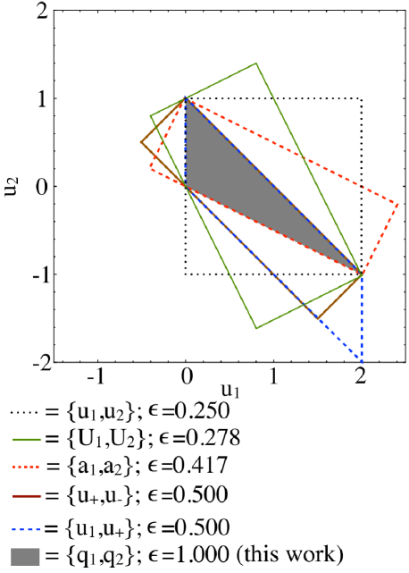
We will therefore proceed by considering several popular parametrizations of the LDCs (in chronological sequence) and evaluating their efficiency, $\epsilon$, and completeness, $\kappa$. During this investigation, we found that it is quite rare for authors to declare the upper and lower bounds used on their priors (which are usually uniform). Without the prior bounds, it is not possible to evaluate $\epsilon$ and $\kappa$ and so in these cases we proceed by selecting a choice of prior bounds which ensures $\kappa=1$ for the highest possible $\epsilon$.

3.4 $\mn@boldsymbol{\theta}=\{u_{1},u_{2}\}$

We begin by first considering the naive parameter set of $\mn@boldsymbol{\theta}=\{u_{1},u_{2}\}$ directly, which serves as a useful baseline for subsequent comparisons. In order to estimate $\kappa$ and $\epsilon$ though, we must first choose upper/lower bounds on these two parameters. As discussed in the previous subsection, we can optimize the prior bounds to ensure $\kappa=1$. This is done by generating $N\gg 1$ Monte Carlo realizations of $\{u_{1},u_{2}\}$ across an overly generous interval (in this case we used $[-3,+3]$) and only accepting points which satisfy the conditions stipulated in equation (8). We find that using $0<u_{1}<+2$ and $-1<u_{2}<+1$ ensures $\kappa=1$ for the highest possible efficiency. The corresponding value of $\epsilon$ is 0.25 i.e. sampling from this prior with a lack of constraining data would mean that three out of four trials would have to be rejected. The parameter volume sampled by this prior is illustrated in Fig. 5.

3.5 $\mn@boldsymbol{\theta}=\{u_{+},u_{-}\}\equiv\{u_{1}+u_{2},u_{1}-u_{2}\}$

The pioneering work of Brown et al. 2001 offers perhaps the first such example of serious consideration of alternative parametrizations in the exoplanet literature. Using the Hubble Space Telescope photometry of HD 209458b, Brown et al. 2001 suggested fitting for $u_{+}\equiv(u_{1}+u_{2})$ and $u_{-}\equiv(u_{1}-u_{2})$. Unlike in this work, the purpose of this parametrization was not to ensure physically plausible intensity profiles, but rather to reduce the correlation between the two LDCs in the fitting procedure, as stated in §3.2 of Brown et al. 2001.

In order to compute our performance metrics, a choice of prior bounds is required. We choose to select these bounds such that we optimize $\kappa=1$, as discussed earlier in §3.3. Following the same method described in §3.4, we estimate that this occurs for $0<u_{+}<+1$ and $-1<u_{-}<+3$. Using these bounds, we calculate that $\epsilon=0.5$. This can be intuitively visualized in Fig. 5.

3.6 $\mn@boldsymbol{\theta}=\{U_{1},U_{2}\}\equiv\{2u_{1}+u_{2},u_{1}-2u_{2}\}$

Holman et al. 2006 chose to fit for $U_{1}\equiv(2u_{1}+u_{2})$ and $U_{2}\equiv(u_{1}-2u_{2})$ because “the resulting uncertainties in those parameters are uncorrelated”. Once again then, it is worth noting that the motivation of this parameter set was not to sample the physically allowed parameter space efficiently. The priors used in the exploration of these parameters are not stated in the paper, and so we assume uniform between some upper and lower bounds on each term. The numerical range is not stated in Holman et al. 2006 but we have learned that the exploration was unbound, but with rejections applied to samples which fall outside of the conditions stated in equation (3), (6) & (7) (private communication with M. Holman & J. Winn).

We therefore proceed by optimizing the prior bound choice to $\kappa=1$ via the same Monte Carlo method described earlier (§3.4). This procedure yields $0<U_{1}<+3$ and $-2<U_{2}<+4$. Using these limits, we calculate $\epsilon=0.278$ for the fixed choice of $\kappa=1$, which is illustrated in Fig. 5.

3.7 $\mn@boldsymbol{\theta}=\{a_{1},a_{2}\}\equiv\{u_{1}+2u_{2},2u_{1}-u_{2}\}$

During our analysis of the literature on this subject, we noticed that the parametrization of Holman et al. 2006 was cited by many authors including the instance of Burke et al. 2007. What is interesting is that Burke et al. 2007 state that ‘we follow Holman et al. 2006 by adopting $a_{1}\equiv(u_{1}+2u_{2})$ and $a_{2}\equiv(2u_{1}-u_{2})$’, but as discussed earlier Holman et al. 2006 in fact used $U_{1}\equiv(2u_{1}+u_{2})$ and $U_{2}\equiv(u_{1}-2u_{2})$. Therefore, despite Burke et al. 2007 claiming to have simply followed Holman et al. 2006, they had in fact introduced an entirely new parametrization. We explore this parametrization here.

Burke et al. 2007 do explicitly declare that they use uniform priors on the LDCs but do not explicitly state the bounds on $a_{1}$ and $a_{2}$. However, the authors do state they impose $u_{1}>0$, $(u_{1}+u_{2})<1$ and $(u_{1}+2u_{2})>0$, which are identical to the conditions derived in this work (see equations 3, 6 & 7). The $a_{1}$ parameter is therefore bound by $a_{1}>0$ but the other constraints do not naturally impose any other bounds. We are also unable to find any way of inferring any other bounds from the paper of Burke et al. 2007.

We therefore proceed by selecting bounds on $a_{1}$ and $a_{2}$ ourselves and we choose parameters which optimize to $\kappa=1$, as discussed in §3.3. Following the same Monte Carlo method used previously (e.g. see §3.4), we determine $0<a_{1}<2$ and $-1<a_{2}<+5$ to ensure $\kappa=1$. Utilizing these bounds, we estimate $\epsilon=(5/12)=0.417$, which is visualized in Fig. 5.

3.8 $\mn@boldsymbol{\theta}=\{w_{1},w_{2}\}\equiv\{u_{1}\cos\phi-u_{2}\sin\phi,u_{1}\sin\phi+u_{2}\cos\phi\}$

Pal 2008 proposed that the correlation between $u_{1}$ and $u_{2}$ can be minimized by using principal component analysis. The author suggested the parametrization $w_{1}\equiv(u_{1}\cos\phi-u_{2}\sin\phi)$ and $w_{2}\equiv(u_{1}\sin\phi+u_{2}\cos\phi)$, where $0<\phi<\pi/2$ and is chosen such that the correlation is minimized. Once again then, we stress that this parametrization is not designed to sample from the physically plausible parameter space. Pal 2008 does not suggest bounds on $w_{1}$-$w_{2}$ and so we proceed to select bounds in such way as to optimize $\kappa=1$. This optimization process is sensitive to $\phi$ though and it is possible to derive different bounds depending upon what one assumes for $\phi$.

In order to explore this issue fully, we fix $\phi$ to a specific value between $0$ and $\pi/2$ and then optimize the bounds on $w_{1}$ and $w_{2}$ to ensure $\kappa=1$, using the same Monte Carlo method employed earlier (e.g. see §3.4). We then use these bounds to compute $\epsilon$ as usual. For each choice of $\phi$ then, we compute a unique value of $\epsilon$, i.e. $\epsilon(\phi)$. Repeating over a wide range of $\phi$ values, we find that $\phi=45^{\circ}$ yields the maximum efficiency of $\epsilon=0.5$ and drops to $\epsilon=0.25$ as one rotates round to $\phi=0^{\circ}$ and $90^{\circ}$.

Setting $\phi=45^{\circ}$ then optimizes the efficiency of sampling the physically plausible parameter space. We stress that this choice is not made to minimize the correlation between $w_{1}$ and $w_{2}$, for which we note Pal 2008 recommend $\phi=35^{\circ}$-$40^{\circ}$. For the $\phi=45^{\circ}$ case, however, $w_{1}=(u_{1}-u_{2})=u_{-}$ and $w_{2}=(u_{1}+u_{2})=u_{+}$, and so we recover the same parametrization used by Brown et al. 2001. For this reason, we do not include the parametrization of Pal 2008 in Fig. 5 and Table 2.

One interesting point is that the boundary conditions in equation (3) and equation (7) form two sides of the triangle described in Fig. 1 and taking the bisector of these two lines yields a line inclined by $\phi=\frac{1}{2}[\tan^{-1}(\frac{1}{2})+\tan^{-1}(\frac{2}{2})]=35.8^{\circ}$, which is also marked in Fig. 1. Therefore, the suggested angle of $\phi=35^{\circ}$-$40^{\circ}$ by Pal 2008 effectively just travels up along this bisector. Indeed, one can consider this to be an alternative geometric explanation for the suggestion of Pal 2008. It also highlights how our parametrization, $\{q_{1},q_{2}\}$, should be expected to exhibit inherently low mutual correlation since it also travels up along this bisector line. This was indeed verified to be the case earlier in §3.2 and here we are able to provide the explicit explanation for this observation.

3.9 $\mn@boldsymbol{\theta}=\{u_{1},u_{+}\}\equiv\{u_{1},u_{1}+u_{2}\}$

The final parametrization we consider is that of $\mn@boldsymbol{\theta}=\{u_{1},u_{+}\}\equiv\{u_{1},u_{1}+u_{2}\}$, which has been used in papers such as Nesvorný et al. 2012 and Kipping et al. 2013. The choice of bounds here is usually stated to be $0<u_{1}<+2$ and $0<(u_{1}+u_{2})<+1$, which incidentally is the same result that one finds when one optimizes the bounds to $\kappa=1$. The loci of points form a parallelogram on the $\{u_{1},u_{2}\}$ plane (as shown in Fig. 5), unlike any of the previously considered parametrizations which formed rectangles (or a triangle in the case of $\mn@boldsymbol{\theta}=\{q_{1},q_{2}\}$) and produces an efficiency of exactly one half i.e. $\epsilon=0.5$. Table 2 shows the efficiency and bounds of this parametrization in relation to previously considered ones.

Table 2: Comparison of the performance metric $\epsilon$ (efficiency) for several different parametrizations of the quadratic LDCs. In each case, the completeness, $\kappa$, equals unity since we have optimized the prior bounds to ensure this condition. This is done since we are unable to find corresponding upper/lower bounds in the referenced literature.

Parametrization, $\mn@boldsymbol{\theta}$	Parameter 1 Interval	Parameter 2 Interval	Efficiency, $\epsilon$
$\{u_{1},u_{2}\}$	$[0,+2]$	$[-1,+1]$	$0.250$
$\{u_{+},u_{-}\}\equiv\{u_{1}+u_{2},u_{1}-u_{2}\}$	$[0,+1]$	$[-1,+3]$	$0.500$
$\{a_{1},a_{2}\}\equiv\{2u_{1}+u_{2},u_{1}-2u_{2}\}$	$[0,+2]$	$[-1,+5]$	$0.417$
$\{U_{1},U_{2}\}\equiv\{u_{1}+2u_{2},2u_{1}-u_{2}\}$	$[0,+3]$	$[-2,+4]$	$0.278$
$\{u_{1},u_{+}\}\equiv\{u_{1},u_{1}+u_{2}\}$	$[0,+2]$	$[0,+1]$	$0.500$
$\{q_{1},q_{2}\}\equiv\{(u_{1}+u_{2})^{2},(u_{1}/2)(u_{1}+u_{2})^{-1}\}$	$[0,+1]$	$[0,+1]$	$1.000$

Figure 5: Loci of points sampled by various parametrizations of the quadratic LDCs. In each case, the completeness, $\kappa$, equals unity since we have optimized the prior bounds to ensure this condition. This is done since we are unable to find corresponding upper/lower bounds in the referenced literature. Grey area represents the physically plausible parameter range.

4 Other Two-Parameter Limb Darkening Laws

4.1 General principle

Although the quadratic limb darkening is the most widely used two-parameter limb darkening in the literature, the so-called ‘square-root’ law and to a lesser extent the ‘logarithmic’ law have also gained traction. Like the quadratic case, enforcing the physical conditions of an everywhere-positive intensity profile and a monotonically decreasing intensity from centre-to-limb imposes three boundary conditions on the two coefficients describing each law. Hence, we once again have a two-dimensional plane featuring three (non-parallel) boundary conditions which enclose a triangle. Therefore, sampling from this triangle in a uniform manner can be achieved using exactly the same trick described for the quadratic law case.

One can actually take this a step further and state that for any problem with two variables with a uniformly distributed joint PDF and three (non-parallel) boundary conditions, 100% complete and efficient sampling is easily achieved using the triangular sampling technique discussed in this paper.

4.2 Square-root law

Arguably, the second-most popular two-parameter limb darkening law is that of the square-root law. van Hamme 1993 argues that this is a superior approximation to the quadratic law for late-type stars in the near-infrared. Recent examples include applications to the eclipsing binary system LSPM J1112+7626 (Irwin et al. 2011) and the transiting planet system GJ 1214 (Berta et al. 2012). The law was first proposed in Diaz-Cordoves & Gimenez 1992 and describes the specific intensity as

$$I(\mu)/I(1) =1-c(1-\mu)-d(1-\sqrt{\mu}),$$ (19)

where $c$ and $d$ are the two LDCs associated with this law. Following the same procedure as used earlier in §2.1, imposing the condition of an everywhere-positive profile yields

$$c+d<1.$$ (20)

Similarly, the condition of a monotonically decreasing intensity profile from centre-to-limb gives two constraints:

$$d>0,$$ (21)

$$2c+d>0.$$ (22)

These three non-parallel conditions are easily imparted using the triangular sampling technique and using the replacements $q_{1}^{\mathrm{sqrt}}$ and $q_{2}^{\mathrm{sqrt}}$ defined over the interval $[0,1]$:

$$q_{1}^{\mathrm{sqrt}} =(c+d)^{2},$$ (23)

$$q_{2}^{\mathrm{sqrt}} =\frac{d}{2(c+d)}.$$ (24)

Alternatively, sampling from uniform, bivariate Dirichlet distribution, $\mathcal{P}(\mn@boldsymbol{\alpha}=\mathbf{1};v_{1}^{\mathrm{sqrt}},v_{2}^{\mathrm{sqrt}})$, may be achieved using:

$$v_{1}^{\mathrm{sqrt}} =d/2,$$ (25)

$$v_{2}^{\mathrm{sqrt}} =1-c-d.$$ (26)

4.3 Logarithmic law

Klinglesmith & Sobieski 1970 proposed a logarithmic limb darkening law with the following form

$$I(\mu)/I(1) =1-A(1-\mu)-B\mu(1-\log\mu),$$ (27)

where $A$ and $B$ are the two associated LDCs. Again, following the procedure used earlier in §2.1, we find that imposing the condition of an everywhere-positive profile yields

$$A<1.$$ (28)

Similarly, the condition of a monotonically decreasing intensity profile from centre-to-limb gives two constraints:

$$A+B>0,$$

$$B<0.$$ (29)

These three non-parallel conditions are again easily imparted using the triangular sampling technique and using the replacements $q_{1}^{\mathrm{log}}$ and $q_{2}^{\mathrm{log}}$ defined over the interval $[0,1]$:

$$q_{1}^{\mathrm{log}} =(B+1)^{2},$$ (30)

$$q_{2}^{\mathrm{log}} =\frac{A-1}{B+1}.$$ (31)

Alternatively, sampling from uniform, bivariate Dirichlet distribution, $\mathcal{P}(\mn@boldsymbol{\alpha}=\mathbf{1};v_{1}^{\mathrm{log}},v_{2}^{\mathrm{log}})$, may be achieved using

$$v_{1}^{\mathrm{log}} =1-A,$$ (32)

$$v_{2}^{\mathrm{log}} =-B.$$ (33)

4.4 Exponential law

The final two-parameter limb darkening law we consider comes from Claret & Hauschildt 2003 and takes the form

$$I(\mu)/I(1) =1-g(1-\mu)-h\frac{1}{1-e^{\mu}},$$ (34)

where $g$ and $h$ are the two associated limb darkening coefficients. Following the procedure used earlier in §2.1 once more, we find that imposing the condition of an everywhere-positive profile yields two constraints (unlike all previous examples where this condition only imposed one meaningful constraint):

$$h<1-e^{1},$$

$$h<0.$$ (35)

However, these two condition are parallel and since $0>(1-e^{1})$, then the two conditions simply boil down to $h<(1-e^{1})$. Similarly, the condition of a monotonically decreasing intensity profile from centre-to-limb gives two constraints:

$$h<0,$$

$$\frac{h_{1}}{h_{2}}>\frac{e^{1}}{(1-e^{1})^{2}}.$$ (36)

The first of these two conditions is parallel to the previously derived constraint of $h<(1-e^{1})$ and in fact less constraining and so we can discard it. In total then, we have only two non-parallel boundary conditions. As a result, a triangular enclosed region is not formed in the joint probability distribution and so the triangular sampling technique discussed in this paper is not applicable.

5 Discussion & Conclusions

In this paper, we have presented new parametrizations for the LDCs of several two-parameter limb darkening laws, including the popular quadratic (§2) and square-root laws (§4.2). When sampled over the interval $[0,1]$, our parametrizations exclusively sample the complete range of physically plausible LDCs (100% efficient and 100% complete). This is twice as efficient as the next best parametrization proposed previously (§3). In the case of the quadratic law, we show that our parametrization also reduces the mutual correlation between the two LDCs (§3.2) with a natural geometric explanation (§3.8), although this was not the motivation behind our formulation.

Fitting astronomical data with our parametrization for the LDCs ensures that all model parameters fully account for one’s ignorance about the stellar intensity profile, leading to more realistic uncertainty estimates. Derived parameters make no assumption about the stellar atmosphere model, except the type of polynomial used to describe it (for which we provide several choices) and that the observations are of normal, main-sequence stars in broad bandpasses. These parametrizations are applicable to any observation affected by limb darkening, such as optical interferometry, microlensing, eclipsing binaries and transiting planets.

Our parametrization may be explained as follows. Requiring the intensity profile to be everywhere-positive and monotonically decreasing from centre-to-limb imposes three non-parallel boundary conditions on two LDCs (see equation 8). Given the two LDCs live on a two-dimensional plane, the three boundary conditions describe a triangular region where physically plausible LDCs may reside. This triangular region can be sampled uniformly by re-parametrizing the LDCs from $\{u_{1},u_{2}\}$ to $\{q_{1},q_{2}\}$ (see equation 18) according to a technique used in computer graphical programming (Turk 1990): triangular sampling. An equivalent method is to draw a random variate from a uniform, bivariate Dirichlet distribution.

We note that the solution is general to any situation where two parameters are bound by three non-parallel boundary conditions. Or, even more generally, when $N$ parameters are mutually constrained by $N+1$ non-parallel boundary conditions leading to tetrahedral sampling and hyper-tetrahedral sampling. In the case of exoplanet transits, we are therefore faced with the unusual case of the field of exoplanets drawing from computer games, rather than the other way around.

References

- Aufdenberg et al. (2005) Aufdenberg, J. P., Ludwig, H.-G. & Kervella, P., 2005, ApJ, 633, 424
- Berta et al. (2012) Berta, Z. K. et al., ApJ, 747, 35
- Brown et al. (2001) Brown, T. M., Charbonneau, D., Gilliland, R. L., Noyes, R. W. & Burrows, A., 2001, ApJ, 552, 699
- Burke et al. (2007) Burke, C. J. et al., 2007, ApJ, 671, 2115
- Carter et al. (2009) Carter, J. A., Winn, J. N., Gilliland, R. & Holman, M. J., 2009, ApJ, 696, 241
- Claret (2000) Claret, A., 2000, A&A, 363, 1081
- Claret & Hauschildt (2003) Claret, A. & Hauschildt, P. H., 2003, A&A, 412, 241
- Claret & Bloemen (2011) Claret, A. & Bloemen, S., 2011, A&A, 529, 75
- Diaz-Cordoves & Gimenez (1992) Diaz-Cordoves, J. & Gimenez, A., 1992, A&A, 259, 227
- van Hamme (1993) van Hamme, W., 1993, AJ, 106, 2096
- Hastings (1970) Hastings, W. K., 1970, Biometrika, 57, 97
- Hayek et al. (2012) Hayek, W., Sing, D., Pont, F. & Apslund, M., 2012, A&A, 539, 1
- Holman et al. (2006) Holman, M. J. et al., 2006, ApJ, 2006, 652, 1715
- Howarth (2011) Howarth, I. D., 2011, MNRAS, 418, 1165
- Irwin et al. (2011) Irwin, J., M. et al., 2011, ApJ, 742, 123
- Kalas et al. (2008) Kalas, P. et al., 2008, Science, 322, 1345
- Kipping (2012) Kipping, D. M., 2012, MNRAS, 427, 2487
- Kipping (2013) Kipping, D. M., 2013, MNRAS, 434, L51
- Kipping et al. (2012) Kipping, D. M., Bakos, G. Á., Buchhave, L. A., Nesvorný, D. & Schmitt, A. R., 2012, ApJ, 750, 115
- Kipping et al. (2013) Kipping, D. M., Hartman, J., Buchhave, L. A., Schmitt, A. R., Bakos, G. Á. & Nesvorný, D., 2013, ApJ, 770, 101
- Kipping et al. (2013) Kipping, D. M., Forgan, D., Hartman, J., Nesvorný, D., Bakos, G. Á., Schmitt, A. R., & Buchhave, L. A., 2013, ApJ, submitted (astro-ph:1306.1530)
- Kjurkchieva et al. (2013) Kjurkchieva, D., Dimitrov, D., Vladev, A. & Yotov, V., 2013, MNRAS, 431, 3654
- Klinglesmith & Sobieski (1970) Klinglesmith, D. A. & Sobiesk, S., 1970, A&A, 75, 175
- Kopal (1950) Kopal, Z., 1950, Harvard Col. Obs. Circ., 454, 1
- Mandel & Agol (2002) Mandel, K. & Agol, E., 2002, ApJ, 580, 171
- Metropolis et al. (1953) Metropolis, N., Rosenbluth, A. W., Rosenbluth, M. N., Teller, A. H. & Teller, E., 1953, J. Chem. Phys., 21, 1087
- Muirhead et al. (2012) Muirhead, P. S. et al., 2012, ApJ, 747, 144
- Neilson & Lester (2012) Neilson, H. R. & Lester, J. B., 2012, A&A, 544, 117
- Nesvorný et al. (2012) Nesvorný, D., Kipping, D. M., Buchhave, L. A., Bakos, G. Á., Hartman, J. & Schmitt, A. R., 2012, Science, 336, 1133
- Pal (2008) Pal, A., 2008, MNRAS, 390, 281
- Schlawin et al. (2010) Schlawin, E., Agol, E., Walkowicz, L. M., Covey, K. & Lloyd, J. P., 2010, ApJ, 722, 75
- Sing (2010) Sing, D. K., 2010, A&A, 510, 21
- Skilling (2004) Skilling, J. 2004, in Fischer R., Preuss R., Toussaint U. V., eds, AIP Conf. Ser. Vol. 735, Nested Sampling. Am. Inst. Phys., p. 395
- Turk (1990) Turk, G., 1990, in Glassmer A., ed., Generating Random Points in a Triangle, in Graphics Gems I. Academic Press, p. 24
- Witt (1995) Witt, J. J., 1995, ApJ, 449, 42
- Zub et al. (2011) Zub, M. et al., 2011, A&A, 525, 15