Estimating magnetic filling factors from Zeeman-Doppler magnetograms

Abstract

Low-mass stars are known to have magnetic fields that are believed to be of dynamo origin. Two complementary techniques are principally used to characterise them. Zeeman-Doppler imaging (ZDI) can determine the geometry of the large-scale magnetic field while Zeeman broadening can assess the total unsigned flux including that associated with small-scale structures such as spots. In this work, we study a sample of stars that have been previously mapped with ZDI. We show that the average unsigned magnetic flux follows an activity-rotation relation separating into saturated and unsaturated regimes. We also compare the average photospheric magnetic flux recovered by ZDI, $\langle B_{V}\rangle$, with that recovered by Zeeman broadening studies, $\langle B_{I}\rangle$. In line with previous studies, $\langle B_{V}\rangle$ ranges from a few % to $\sim$20% of $\langle B_{I}\rangle$. We show that a power law relationship between $\langle B_{V}\rangle$ and $\langle B_{I}\rangle$ exists and that ZDI recovers a larger fraction of the magnetic flux in more active stars. Using this relation, we improve on previous attempts to estimate filling factors, i.e. the fraction of the stellar surface covered with magnetic field, for stars mapped only with ZDI. Our estimated filling factors follow the well-known activity-rotation relation which is in agreement with filling factors obtained directly from Zeeman broadening studies. We discuss the possible implications of these results for flux tube expansion above the stellar surface and stellar wind models.

1. Introduction

Over the last two decades, our understanding of stellar magnetism has been enriched by Zeeman-Doppler imaging (ZDI; Donati & Landstreet, 2009). This is a tomographic technique that can reconstruct the large-scale photospheric magnetic field topology of low-mass stars from a time-series of high-resolution polarised spectra sampling at least one stellar rotation. (Semel, 1989; Brown et al., 1991; Donati & Brown, 1997; Donati et al., 2006). Repeated observations of individual stars show that their magnetic fields are inherently variable (Morgenthaler et al., 2012; Jeffers et al., 2014; Boro Saikia et al., 2015; Mengel et al., 2016; Fares et al., 2017; Jeffers et al., 2017) and can show regular global polarity reversals similar to those of the Sun (Donati et al., 2008b; Fares et al., 2009, 2013; Boro Saikia et al., 2016; Mengel et al., 2016; Jeffers et al., 2018; Boro Saikia et al., 2018). Additionally, ensemble studies, that utilise samples consisting of between a handful of stars to nearly 100, have shown that the magnetic properties of low-mass stars depend on fundamental stellar parameters such as mass and rotation (Petit et al., 2008; Donati et al., 2008a; Morin et al., 2008a, 2010; Vidotto et al., 2014; See et al., 2015, 2016; Folsom et al., 2016, 2018b).

Although ZDI is capable of reconstructing the large-scale component of stellar magnetic fields, it is insensitive to small-scale fields, e.g. those associated with magnetic spots. This is because the ZDI technique utilises circularly polarised light (Stokes V) which is known to suffer from flux cancellation effects (Morin et al., 2010; Johnstone et al., 2010; Arzoumanian et al., 2011; Lang et al., 2014). A number of authors have studied the link between the large- and small-scale fields by using numerical models (Yadav et al., 2015; Lehmann et al., 2017, 2018) or solar magnetograms (Vidotto, 2016; Vidotto et al., 2018).

In contrast to ZDI, Zeeman broadening observations make use of unpolarised light (Stokes I) that does not suffer from flux cancellation. The disadvantage of using Zeeman broadening is that it is insensitive to magnetic topology. Therefore, ZDI and Zeeman broadening are complementary techniques and both are required to build a holistic picture of stellar magnetism (see Reiners, 2012, for a summary). Zeeman broadening studies typically express the average unsigned surface field strength, $\langle B_{I}\rangle$, in terms of a photospheric field strength, $B$, multiplied by a filling factor, $f$, or a combined $Bf\equiv\langle B_{I}\rangle$ value (Johns-Krull & Valenti, 1996; Reiners & Basri, 2007; Phan-Bao et al., 2009; Reiners et al., 2009a). Conceptually, $f$ can be thought of as the fraction of the stellar surface filled with magnetic field of strength $B$, with the remaining area, $1-f$, having zero magnetic field. The photospheric field strength, $B$, is thought to be roughly equal to the equipartition field strength (Saar & Linsky, 1986). However, this interpretation is a simplification as studies have shown that Stokes I observations can be fit with multiple magnetic components of different field strengths, each with their own associated filling factors, i.e. $\langle B_{I}\rangle\equiv\sum_{i}B_{i}f_{i}$ (Johns-Krull, 2007; Yang et al., 2008; Shulyak et al., 2014). Field strengths of up to $\langle B_{I}\rangle\sim\ 7{\rm kG}$ have been reported (Shulyak et al., 2017) which is well in excess of any surface averaged field strength obtained by ZDI for cool stars. Indeed, comparisons of stars that have been analysed with both Zeeman broadening and ZDI show that the large-scale magnetic flux, to which spectropolarimetry is sensitive, only represents a small fraction of the total magnetic flux (Reiners & Basri, 2009; Morin et al., 2010). Additionally, the rate at which field lines expand with height above the stellar surface is known to affect stellar wind properties (Wang & Sheeley, 1990; Suzuki, 2006; Pinto et al., 2016). This rate of expansion is difficult to predict but knowledge of magnetic filling factors can help with this problem (Cranmer & Saar, 2011).

In this work, we compare the magnetic properties of low-mass stars inferred from Zeeman broadening to those inferred from ZDI. We present a sample of stars that have previously been mapped with ZDI in section 2. In section 3, we discuss the magnetic properties of our sample. We present the unsigned magnetic fluxes obtained using ZDI (section 3.1), compare the magnetic field properties of stars that have been observed using both Zeeman broadening and ZDI (section 3.2) and infer filling factors for our ZDI sample (section 3.3). Conclusions are presented in section 4.

2. Sample

In this work, we use a sample of 85 low-mass stars that have had their large-scale photospheric magnetic fields reconstructed with ZDI. A number of these stars have been observed at multiple epochs resulting in a total of 151 magnetic maps in the sample. Many of the ZDI maps come from the efforts of the BCool (Petit et al., in prep) and Toupies (Folsom et al., 2016, 2018b) collaborations. These stars have a wide range of fundamental parameters with spectral types spanning F, G, K & M and have rotation periods from fractions of a day to several tens of days. A full list of the stars used can be found in table 1 along with the average unsigned photospheric flux derived from ZDI, $\langle B_{V}\rangle$, and references to the original paper for each map. The masses, radii, luminosities and rotation periods of each star are also listed in table 1. Unless otherwise noted, these values are taken from the original ZDI publication, Valenti & Fischer (2005), Takeda et al. (2007) or from Vidotto et al. (2014) and references therein. In some cases, the bolometric luminosities have been calculated using the $L_{\rm X}/L_{\rm bol}$ and $L_{\rm X}$ values listed in Vidotto et al. (2014). Rossby numbers are given by the rotation period divided by the convective turnover time. Convective turnover times are calculated in the manner described by Cranmer & Saar (2011) and are a function of effective temperature (see their equation (36)) with an additional weak dependence on the surface gravity for stars with surface gravities smaller than that of the Sun. Finally, $\langle B_{I}\rangle$ values were available for a subset of the stars in this sample from the literature. These values are listed in table 2 along with references for the paper in which they were published.

3. Magnetic properties

3.1. Zeeman-Doppler imaging

ZDI reconstructs the radial, meridional and azimuthal components of the large-scale photospheric stellar magnetic field. Although each map contains a wealth of information, it is common to reduce each map to a set of numerical values that capture the global magnetic field characteristics. In this work, we will use the average unsigned photospheric magnetic flux, $\langle B_{V}\rangle$. This is calculated by taking an average of the absolute value of the magnetic field strength over the stellar surface and accounts for all three components of the magnetic field, i.e. radial, meridional and azimuthal.

In fig. 1, we plot $\langle B_{V}\rangle$ against Rossby number. The $\langle B_{V}\rangle$ values follow the well-known activity-rotation relation shape from studies of other magnetic activity indicators including, but not limited to, X-ray emission (Pizzolato et al., 2003; Wright et al., 2011; Wright & Drake, 2016; Stelzer et al., 2016; Wright et al., 2018), i.e. a roughly constant field strength in the so called “saturated regime” at small Rossby numbers and a power law relation in the so called “unsaturated regime” at large Rossby numbers. This is also similar to results found in previous works analysing the relationship between magnetic field properties derived from ZDI and Rossby number (Vidotto et al., 2014; See et al., 2015; Folsom et al., 2016; See et al., 2017; Folsom et al., 2018b). Additionally, we plot a magenta strut to represent the solar range of $\langle B_{V}\rangle$ values. This range was calculated using a set of solar magnetograms studied by Vidotto et al. (2018) that cover most of solar cycle 24. Since ZDI only recovers the large-scale magnetic field components, the solar magnetograms were truncated to a spherical harmonic order of $\ell_{\rm max}=5$ to provide a more fair comparison (see Vidotto et al. (2018) for more details). A mean photospheric field strength is derived for each solar magnetogram with the strut representing the range of field strengths seen in these magnetograms.

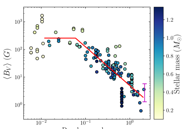
Figure 1.— Average unsigned photospheric magnetic flux obtained from ZDI against Rossby number colour coded by stellar mass. The three parameter fit (solid red line) has a saturated field strength of $\langle B_{V}\rangle_{\rm sat}=257\pm 72$G, a critical Rossby number of $\rm Ro_{crit}=0.06\pm 0.01$ and an unsaturated regime slope value of $\beta=-1.40\pm 0.10$. The magenta strut represents the range of $\langle B_{V}\rangle$ values over cycle 24 (the magnetograms used to calculate this range were truncated to $\ell_{\rm max}=5$; see text and Vidotto et al. (2018) for more details).

We perform a three parameter fit to the data of the form

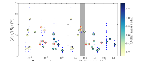
Figure 2.— $\langle B_{V}\rangle$ as a percentage of $\langle B_{I}\rangle$ against Rossby number (left) and stellar mass (right). Average values for $\langle B_{I}\rangle$ and $\langle B_{V}\rangle$ for each star are shown with large points colour coded by stellar mass. The six stars in the study of Reiners & Basri (2009) are outlined in red. All permutations of $\langle B_{I}\rangle$ and $\langle B_{V}\rangle$ for each star are shown with small blue points (see text). The shaded region in the right hand panel indicates the transition to full convection ($\sim 0.35M_{\odot}$).

$$\begin{split}\langle B_{V}\rangle&=\langle B_{V}\rangle_{\rm sat}\hskip 65.44133pt{\rm for\ Ro<Ro_{crit}}\\ \langle B_{V}\rangle&=\langle B_{V}\rangle_{\rm sat}\left(\frac{\rm Ro}{\rm Ro_{crit}}\right)^{\beta}\hskip 14.22636pt{\rm for\ Ro\geq Ro_{crit}}\end{split}$$ (1)

where $\langle B_{V}\rangle_{\rm sat}$ is the field strength in the saturated regime, $\rm Ro_{crit}$ is the critical Rossby number dividing the saturated and unsaturated regimes and $\beta$ is the power law index of the unsaturated regime. We find best fit values of $\langle B_{V}\rangle_{\rm sat}=257\pm 72$G, $\rm Ro_{crit}=0.06\pm 0.01$ and $\beta=-1.40\pm 0.10$ (shown in fig. 1 as a solid red line). The power law slope is relatively well constrained because the majority of data points fall in the unsaturated regime ($\sim$130 maps) and is consistent with the value of $\beta=-1.38\pm 0.14$ found by Vidotto et al. (2014). However, $\langle B_{V}\rangle_{\rm sat}$ is less well constrained because there are comparatively few stars in the saturated regime. It is worth noting that the lowest mass stars with the smallest Rossby numbers ($\rm Ro\lesssim 0.012$) have bimodal magnetic fields as previously noted in the literature (Morin et al., 2010). It is clear that these low Rossby number stars are comprised of two sub-groups; one with high field strengths and one with low field strengths. A number of explanations have been proposed for this bimodality (Morin et al., 2011; Gastine et al., 2013; Kitchatinov et al., 2014). However, there is, as of yet, no consensus and as such, we have excluded these stars from the three parameter fit. Although we have chosen to fit a single saturation level to this data, it is also worth noting that two saturation plateaus may exist if one considers the early-M and mid-M dwarfs separately (see discussion in Vidotto et al., 2014).

An interesting result is the small value we obtain for $\rm Ro_{crit}$. Previous works studying the relationship between different activity indicators and Rossby number typically find critical Rossby numbers that are larger. For example, Douglas et al. (2014) and Newton et al. (2017) find $\rm Ro_{crit}=0.11^{+0.02}_{-0.03}$ and $\rm Ro_{crit}=0.21\pm 0.02$ respectively when studying $H\alpha$ emission from different samples, while Wright et al. (2011) find $\rm Ro_{crit}=0.13\pm 0.02$ when studying X-ray emission. This discrepancy could be due to a number of reasons. For example, we have already noted that the saturation field strength is relatively unconstrained. A larger critical Rossby number could result if the saturation value were lower. Alternatively, differences in the way the convective turnover times, which are notoriously hard to estimate, may contribute to the discrepancy. Lastly, the different $\rm Ro_{crit}$ values may reflect the fact that some of these studies are measuring secondary processes, e.g. X-ray emission, that have non-linear dependencies on the magnetic field strength. As such, it is not obvious that different activity indicators should saturate at the same Rossby number (also see Jardine & Unruh, 1999, and references therein). Further work is required to establish whether the different estimates for $\rm Ro_{crit}$ reflects a real difference in the Rossby number at which large-scale magnetic fields saturate compared to other activity indicators. However, a full comparison of $\rm Ro_{crit}$ values using different activity indicators is beyond the scope of the current work. Finally, we also note that Reiners et al. (2014) suggest that rotation period may be a more relevant parameter compared to Rossby number in the context of magnetic activity.

3.2. Zeeman broadening vs ZDI

A growing number of stars have been studied with both ZDI and Zeeman broadening techniques. For each star in our ZDI sample, we search for $\langle B_{I}\rangle$ values in the literature. This resulted in 21 stars that have at least one $\langle B_{V}\rangle$ value and one $\langle B_{I}\rangle$ value. We have listed the $\langle B_{I}\rangle$ values in table 2. We caution that the $\langle B_{I}\rangle$ values listed in table 2 and the $\langle B_{V}\rangle$ values listed in table 1 were not observed simultaneously for any of the stars and this will add some scatter to our plots due to magnetic variability. We also note that these values originate from different authors who have used different models and assumptions that will add an additional level of scatter.

There have been relatively few comparisons between Zeeman broadening observations and ZDI observations in the literature. Reiners & Basri (2009) and Morin et al. (2010) compared magnetic field measurements from the two techniques for M stars. A number of key results emerged from these studies. The first is that ZDI only captures a small fraction of the total magnetic flux when compared to Zeeman broadening. The second is that $\langle B_{V}\rangle/\langle B_{I}\rangle$ increases by a factor of $\sim 2$ as one crosses the fully convective boundary ($\sim 0.35M_{\odot}$) from partially to fully convective stars. In fig. 2 we plot $\langle B_{V}\rangle$ as a percentage of $\langle B_{I}\rangle$ against Rossby number and stellar mass with the points colour coded by stellar mass. This is similar to the middle panels of figure 2 from Reiners & Basri (2009). Some of the stars have multiple $\langle B_{V}\rangle$ values, multiple $\langle B_{I}\rangle$ values or multiple of both. In these cases, we used averaged $\langle B_{V}\rangle$ or $\langle B_{I}\rangle$ values. The six stars that were used in the study of Reiners & Basri (2009) are outlined in red. Additionally, for each star, we also plot all the combinations of $\langle B_{I}\rangle$ and $\langle B_{V}\rangle$ with small blue points. For instance, if a star has $m$ number of $\langle B_{I}\rangle$ values and $n$ number of $\langle B_{V}\rangle$ values, it will have a column of $m\times n$ number of blue points around its averaged value in fig. 2. This visually illustrates the scatter that may exist due to magnetic variability and the fact that the $\langle B_{I}\rangle$ and $\langle B_{V}\rangle$ observations were not simultaneous.

Compared to the studies of Reiners & Basri (2009) and Morin et al. (2010), ours includes a greater number of stars that span a larger range in stellar mass. Similarly to these studies, we find that the reconstructed $\langle B_{V}\rangle$ value is between a few % to $\sim 20\%$ of the $\langle B_{I}\rangle$ value. The second result, that $\langle B_{V}\rangle/\langle B_{I}\rangle$ changes by a factor of $\sim$2 across the full convective boundary, still persists but is not as clear in our larger sample. The five stars with masses around or just below the fully convective limit ($M_{\star}\lesssim 0.35M_{\odot}$; EV Lac, GJ 285, V374, Peg EQ Peg A & EQ Peg B) all have very similar $\langle B_{V}\rangle/\langle B_{I}\rangle$ values (around 10% - 13%) in line with the results of Reiners & Basri (2009) and Morin et al. (2010). The majority of the partially convective stars have lower average $\langle B_{V}\rangle/\langle B_{I}\rangle$ values compared to these 5 fully (or nearly fully) convective stars but there are a few stars worth discussing in more detail. $\epsilon$ Eri ($0.86M_{\odot}$) and $\xi$ Boo A ($0.93M_{\odot}$) both have a large range of $\langle B_{V}\rangle/\langle B_{I}\rangle$ values; 3% to 15% for $\epsilon$ Eri and 4% to 18% for $\xi$ Boo A depending on the combination of $\langle B_{V}\rangle$ and $\langle B_{I}\rangle$ values used for each star. The upper values of these $\langle B_{V}\rangle/\langle B_{I}\rangle$ ranges are larger than those for the five fully (or nearly fully) convective stars and would seemingly invalidate the conclusion that partially convective stars have lower $\langle B_{V}\rangle/\langle B_{I}\rangle$ values. However, this range of $\langle B_{V}\rangle/\langle B_{I}\rangle$ values is likely to be an overestimate due to the non-simultaneous observations used to derive the individual $\langle B_{V}\rangle$ and $\langle B_{I}\rangle$ values. The true range of possible $\langle B_{V}\rangle/\langle B_{I}\rangle$ values is unlikely to be as high or low as suggested by the blue points in fig. 2. Notably, the average $\langle B_{V}\rangle/\langle B_{I}\rangle$ values of 8.2% for $\xi$ Boo A and 6.9% for $\epsilon$ Eri are roughly in line with the rest of the partially convective stars. The last star worth briefly discussing is DS Leo ($0.58M_{\odot}$) which has the highest average $\langle B_{V}\rangle/\langle B_{I}\rangle$ value of 10.5% of the partially convective stars. This is comparable to $\langle B_{V}\rangle/\langle B_{I}\rangle$ for the five previously discussed fully (or nearly fully) convective stars. Given that it is the only partially convective star with such a high average $\langle B_{V}\rangle/\langle B_{I}\rangle$ value, it is unclear if the individual $\langle B_{V}\rangle$ and $\langle B_{I}\rangle$ values are discrepent in some way. Simultaneous Stokes I and Stokes V measurements would be useful to determine whether the $\langle B_{V}\rangle/\langle B_{I}\rangle$ value for DS Leo is truly this high.

At the lowest masses ($\lesssim 0.2M_{\odot}$), we see a wide range $\langle B_{V}\rangle/\langle B_{I}\rangle$ values. These stars are a subset of the bimodal $\rm Ro\lesssim 0.12$ stars discussed in section 3.1. As noted by Morin et al. (2010) the magnetic fields of these stars are either strong and dipole dominated or comparatively weak and multipolar. These authors also showed that the bimodality is evident when considering $\langle B_{V}\rangle/\langle B_{I}\rangle$. WX UMa, which is a strong field dipolar star, has an average $\langle B_{V}\rangle/\langle B_{I}\rangle$ value of 18%. On the other hand, DX Cnc, GJ 1245b and GJ 1156, which are all weak field stars, have average $\langle B_{V}\rangle/\langle B_{I}\rangle$ values of $\sim$4%. Lastly, we note that the upper envelope of $\langle B_{V}\rangle/\langle B_{I}\rangle$ points in the left panel of fig. 2 decreases with Rossby number. As noted by Morin et al. (2010), this may be because all the fully convective stars have small Rossby numbers.

Figure 3.— Average unsigned photospheric magnetic field strengths obtained from Zeeman broadening, $\langle B_{I}\rangle$, and ZDI, $\langle B_{V}\rangle$. Symbols have the same meaning as fig. 2. Stars less massive than 0.5$M_{\odot}$ are shown with pentagons. A best fit line to all the averaged values is shown in red and is given by $\langle B_{I}\rangle=(61\pm 17)\langle B_{V}\rangle^{0.70\pm 0.06}$. Fits to stars less massive than 0.5$M_{\odot}$ and more massive than 0.5$M_{\odot}$ are shown with purple dashed lines and are given by $\langle B_{I}\rangle=(329\pm 79)\langle B_{V}\rangle^{0.42\pm 0.04}$ and $\langle B_{I}\rangle=(41\pm 18)\langle B_{V}\rangle^{0.78\pm 0.12}$ respectively. The black dotted line indicates where $\langle B_{I}\rangle=\langle B_{V}\rangle$.

In fig. 3, we plot $\langle B_{I}\rangle$ directly against $\langle B_{V}\rangle$. The symbols have the same meanings as in fig. 2 (the small blue points form a cloud around the average point rather than a column in this parameter space). A clear relation between $\langle B_{V}\rangle$ and $\langle B_{I}\rangle$ seems to exist. We fit a power law relation to the average points and find that it has the form

$$\langle B_{I}\rangle=(61\pm 17)\langle B_{V}\rangle^{0.70\pm 0.06},$$ (2)

where $\langle B_{I}\rangle$ and $\langle B_{V}\rangle$ are both in units of Gauss. This is shown by a solid red line in fig. 3. Again, it is clear that ZDI does not recover all the photospheric flux when comparing the data points to the black dotted line that indicates $\langle B_{I}\rangle=\langle B_{V}\rangle$. Taken at face value, equation (2) means that ZDI recovers a larger fraction of the photospheric field for more active stars, i.e. those with larger $\langle B_{V}\rangle$. Rearranging equation (2), we find $\langle B_{V}\rangle/\langle B_{I}\rangle\propto\langle B_{V}\rangle^{0.29}$. One interpretation is that more active stars may store a smaller fraction of their magnetic energy in small scale structures. Petit et al. (2008) suggested a similar interpretation based on their analysis of the ZDI maps and chromospheric activities of a sample of four stars. This is also backed up by dynamo models that find that the fraction of field in the dipole component goes up for more rapidly rotating, or equivalently, more active, stars (see discussion in section 6.4 of Brun & Browning (2017)). If this is true, one might speculate that a higher proportion of the surface magnetic flux is opened up into open flux for more active stars since the open flux is dominated by the large-scale field components (e.g. Jardine et al., 2017). This has implications for calculating stellar angular momentum-loss rates that have been shown to be strongly dependent on the open flux (Réville et al., 2015; Pantolmos & Matt, 2017; Finley & Matt, 2017, 2018). On the other hand, this trend may, at least partially, be explained by biases in the ZDI technique since ZDI recovers more small-scale structure for stars with larger $v$sin$i$ (Morin et al., 2010).

An intriguing possibility is that the data points in fig. 3 can be better fit by two separate power laws. As well as the fit to all the data points given by equation (2), we perform two additional fits to the stars above and below 0.5$M_{\odot}$ separately. These are shown by the dashed purple lines and are given by

$$\langle B_{I}\rangle=(41\pm 18)\langle B_{V}\rangle^{0.78\pm 0.12}$$ (3)

and

$$\langle B_{I}\rangle=(329\pm 79)\langle B_{V}\rangle^{0.42\pm 0.04}$$ (4)

respectively. It is apparent, from fig. 3, that the two fits have two different power law slopes. A number of authors have previously discussed a change in the magnetic properties derived from ZDI at 0.5$M_{\odot}$ (Donati et al., 2008a; Morin et al., 2008a, 2010; Gregory et al., 2012; See et al., 2015). For example, See et al. (2015) showed that the energy stored in the toroidal component of the magnetic field increases more steeply as a function of the poloidal magnetic energy for $M_{\star}>0.5M_{\odot}$ stars compared to $M_{\star}<0.5M_{\odot}$ stars (see their fig. 2). This break is very roughly coincident with the mass at which stars become fully convective and may be linked with the change in internal structure. Of course, the two fits are performed on a relatively small number of points and more data will be required to confirm whether the data is truly better fit by two separate power laws. Additionally, we caution that any estimate of $\langle B_{I}\rangle$ from $\langle B_{V}\rangle$ using equations (2), (3) or (4) is only very approximate due to the limited number of data points, the sources of uncertainty discussed previously and intrinsic variability that should be addressed with long-term simultaneous Stokes I and Stokes V monitoring of these stars.

3.3. Estimating filling factors

As discussed in the introduction, $\langle B_{I}\rangle$ can be interpreted as a fraction of the stellar surface, $f$, filled with magnetic field of strength $B$ (Reiners, 2012). Cranmer & Saar (2011) showed that the field strength, $B$, is roughly equal to the equipartition field strength, i.e. the field strength that corresponds to balanced magnetic and gas pressures. These authors also showed that the filling factor, $f$, scales with Rossby number following an activity-rotation relation type behaviour. In contrast, ZDI reconstructs magnetic field over the entire stellar surface. There have already been attempts to estimate filling factors for stars based only on ZDI observations. For instance, Cranmer (2017) showed that, by scaling ZDI field strengths by a factor of 7 to account for the flux missed by ZDI, the inferred filling factors are roughly compatible with those found from Zeeman broadening (see their fig. 4). However, these authors note that a more physically motivated correction method could be more appropriate.

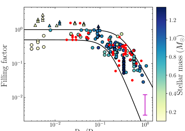
Figure 4.— Filling factor against Rossby number normalised to the solar Rossby number. The data points of Cranmer & Saar (2011) are shown in red while their bounding curves are shown in black (see their figure 7b). The range of filling factors exhibited by the Sun, as estimated by Cranmer (2017), is shown with a magenta strut. The estimated filling factors of the ZDI sample are shown with the coloured points colour coded by stellar mass. Stars with estimated filling factors larger than 1 are shown with triangular points.

In this section, we will estimate filling factors for our ZDI sample using the following procedure. Using equation (2) and the $\langle B_{V}\rangle$ value of each ZDI map, we estimate the average surface field strength that Zeeman broadening observations would have retrieved, $\langle B_{I}\rangle_{\rm est}\ (\equiv B_{\rm est}f_{\rm est})$. We prefer to use equation (2) rather than equations (3) and (4) since it is not clear whether two separate power law fits are truly justified with the current data. We assume that $B_{\rm est}$ is given by 1.13 times the equipartition field strength following the approach of Cranmer & Saar (2011, see section 2.1 of their paper for more details). Using this method, $B_{\rm est}$ scales with the square root of the photospheric density and effective temperature. For our sample, it ranges from $\sim$4kG for the lowest mass stars to $\sim$1kG for the largest. Filling factors are then given by dividing $\langle B_{I}\rangle_{\rm est}$ by $B_{\rm est}$ and are shown in fig. 4. We also show filling factors inferred from Zeeman broadening (red points), bounding envelopes from Cranmer & Saar (2011, black curves) and the estimated range of the solar filling factor from Cranmer (2017, magenta strut) in fig. 4.

Our estimated filling factors broadly follow the activity-rotation relation shape and fall mostly within the two envelopes identified by Cranmer & Saar (2011). On average, more active stars have larger estimated filling factors. This has possible implications for the dynamics of stellar winds. For instance, it is known that the rate at which flux tubes expand can affect stellar wind properties (Wang & Sheeley, 1990; Suzuki, 2006; Pinto et al., 2016). The wind carrying flux tubes of more active stars that have larger filling factors are likely to have smaller expansion factors since less expansion is required to fill the circumstellar volume. Care should be taken with this interpretation however because the relevant parameter for stellar winds is the filling factor associated with open flux tubes. In general, this is only a fraction of the total filling factor that we have estimated here. On the Sun, the filling factor of open flux is correlated with the total filling factor over the solar cycle (equation 7 of Cranmer, 2017) but it is not known whether this relation holds over the course of a cycle on other stars or from star to star.

This method of estimating filling factors from ZDI observations is similar to that of Cranmer (2017). However, rather than a constant scaling factor of 7 to account for the flux missed by ZDI, we use one that is a function of $\langle B_{V}\rangle$. Our scaling factors, given by re-arranging equation (2) for $\langle B_{I}\rangle/\langle B_{V}\rangle$, range from roughly 60 to 8 for $\langle B_{V}\rangle$ = 1G to 1kG respectively. This method is likely to be more robust than using a constant scaling factor since it is calibrated using stars that have both ZDI and Zeeman broadening observations. This is reflected in the fact that the majority of the estimated filling factors are roughly consistent with those inferred from Zeeman broadening observations. However, there is still room for improvement. Notably, this method estimates filling factors that are larger than 1 for some of our stars at small Rossby numbers (plotted as triangles in fig. 4) which is clearly unphysical. One area of our analysis that could be improved in the future is the assumption that the stellar surface is only covered with either equipartition field or zero field. In reality, the photospheric magnetic field is likely to be highly structured and to have a range of field strengths. Indeed, some observations imply local field strengths that exceed the equipartition field strength (Morin et al., 2010; Shulyak et al., 2014). Notably, Okamoto & Sakurai (2018) recently reported an observed field strength of 6.25 kG on the Sun, a value that is roughly four times stronger than equipartition. The fact that we have obtained filling factors larger than 1 could be explained by the lack of super-equipartition field strengths in our calculations. However, it is currently unclear how real magnetic field strengths are distributed on other stars and so we choose to use this simpler model.

4. Conclusions

We have analysed and compared the magnetic properties of low-mass stars derived from two observational techniques. The first is Zeeman-Doppler imaging which is capable of reconstructing the large-scale magnetic field geometry using circularly polarised light (Stokes V) but is insensitive to small-scale magnetic field structures such as spots. The second is Zeeman broadening observations which can assess the field down to the smallest scales using unpolarised light (Stokes I) but cannot assess field geometry.

In this work, we present the average photospheric unsigned flux from ZDI observations and showed that it follows the well known activity-rotation relation type scaling. There are indications that the critical Rossby number at which the magnetic field strength saturates is smaller than the critical Rossby number from other magnetic activity indicators. In line with previous studies, we confirm that ZDI reconstructs between a few % and $\sim$20% of the photospheric magnetic flux and that ZDI seems to recover a smaller percentage of the magnetic flux in partially convective stars than in fully convective stars. At the lowest masses ($\lesssim 0.2M_{\odot}$), there is a large spread in the percentage of magnetic flux that ZDI recovers due to stars with bimodal magnetic fields (Morin et al., 2010).

We find a clear power law relation between the average magnetic fluxes recovered from ZDI and those recovered from Zeeman broadening. There is also a hint that this relationship may be better fit with two separate power laws; one for stars with $M_{\star}<0.5M_{\odot}$ and one for stars with $M_{\star}>0.5M_{\odot}$. However, this suggesting requires more data to confirm, especially for low-mass slow rotators and high-mass fast rotators, which are under-represented in our sample. We use this power law relation to estimate the filling factors for stars that only have ZDI observations. This builds on previous work that has attempted to infer filling factors from ZDI maps (Cranmer, 2017). We show that this method produces filling factor estimates that are similar to those obtained from Zeeman broadening studies. These relations allow for a rough assessment of the amount of flux that any given ZDI map may be missing due to flux cancellation effects and will also be helpful for future stellar wind studies. This is because the amount that flux tubes expand above the stellar surface, which depends on the amount of the stellar surface covered in magnetic regions, affects the dynamics of stellar winds (Wang & Sheeley, 1990). However, distinguishing the filling factor associated with open flux tubes from the total filling factor remains a challenging task. In the future, our understanding of the relationship between ZDI and Zeeman broadening observations should be improved by the new spectropolarimeter, SPIRou (e.g. Moutou et al., 2017), which will be capable of simultaneous ZDI and Zeeman broadening observations.

Table 1Stellar parameters for our ZDI sample. Listed are the stellar mass, radius, luminosity, rotation period, Rossby number, average field strength from ZDI, estimated filling factors (see section 3.3) and the original publication of the ZDI map. Unless otherwise noted, stellar parameters were taken from the original ZDI publication, Valenti & Fischer (2005), Takeda et al. (2007) or Vidotto et al. (2014) and reference therein.

Star	$M_{\star}$	$r_{\star}$	$L_{\star}$	$P_{\rm rot}$	Ro	$\langle B_{V}\rangle$	$f_{\rm est}$	Reference
ID	($M_{\odot}$)	($r_{\odot}$)	($L_{\odot}$)	(d)		(G)
HD 3651	0.88	0.88	0.52	43.4	2.1	3.58	0.085	Petit et al. (in prep)
HD 9986	1.02	1.04	1.1	23	1.8	0.605	0.029	Petit et al. (in prep)
HD 10476	0.82	0.82	0.43	16	0.74	1.98	0.055	Petit et al. (in prep)
$\kappa$ Cet	1.03	0.95	0.83	9.3	0.62	23.6	0.34	do Nascimento et al. (2016)
$\epsilon$ Eri (2007)	0.86	0.74	0.33	10.3	0.45	11.8	0.18	Jeffers et al. (2014)
$\epsilon$ Eri (2008)	0.86	0.74	0.33	10.3	0.45	9.5	0.15	Jeffers et al. (2014)
$\epsilon$ Eri (2010)	0.86	0.74	0.33	10.3	0.45	15.6	0.22	Jeffers et al. (2014)
$\epsilon$ Eri (2011)	0.86	0.74	0.33	10.3	0.45	9.84	0.16	Jeffers et al. (2014)
$\epsilon$ Eri (2012)	0.86	0.74	0.33	10.3	0.45	18.3	0.24	Jeffers et al. (2014)
$\epsilon$ Eri (2013)	0.86	0.74	0.33	10.3	0.45	19.5	0.25	Jeffers et al. (2014)
HD 39587	1.03	1.05	1.1	4.83	0.38	18.5	0.32	Petit et al. (in prep)
HD 56124	1.03	1.01	1.1	18	1.5	2.19	0.07	Petit et al. (in prep)
HD 72905	1	1	1.1	5	0.44	27.7	0.42	Petit et al. (in prep)
HD 73350	1.04	0.98	0.95	12.3	0.93	11	0.21	Petit et al. (2008)
HD 75332	1.21	1.24	2.1	4.8	0.99	6.2	0.18	Petit et al. (in prep)
HD 76151	1.06	1	0.97	20.5	1.5	2.99	0.083	Petit et al. (2008)
HD 78366	1.13	1.06	1.2	11.4	1.1	12.3	0.24	Petit et al. (in prep)
HD 101501	0.85	0.9	0.61	17.6	0.94	12.4	0.21	Petit et al. (in prep)
$\xi$ Boo A (2007)	0.93	0.84	0.52	6.4	0.33	61.8	0.6	Morgenthaler et al. (2012)
$\xi$ Boo A (2008)	0.93	0.84	0.52	6.4	0.33	22.2	0.29	Morgenthaler et al. (2012)
$\xi$ Boo A (2009)	0.93	0.84	0.52	6.4	0.33	36.5	0.42	Morgenthaler et al. (2012)
$\xi$ Boo A (Jan 2010)	0.93	0.84	0.52	6.4	0.33	29.3	0.36	Morgenthaler et al. (2012)
$\xi$ Boo A (Jun 2010)	0.93	0.84	0.52	6.4	0.33	24.3	0.31	Morgenthaler et al. (2012)
$\xi$ Boo A (Jul 2010)	0.93	0.84	0.52	6.4	0.33	35.6	0.41	Morgenthaler et al. (2012)
$\xi$ Boo A (2011)	0.93	0.84	0.52	6.4	0.33	37.9	0.43	Morgenthaler et al. (2012)
$\xi$ Boo B	0.7a	0.55b	0.097a	10.3	0.3	16.3	0.18	Petit et al. (in prep)
18 Sco	1.01	1.04	1.1	22.7	1.7	1.18	0.045	Petit et al. (2008)
HD 166435	1.04	0.99	0.99	3.43	0.27	20	0.32	Petit et al. (in prep)
HD 175726	1.06	1.06	1.2	3.92	0.38	9.62	0.21	Petit et al. (in prep)
HD 190771	1.06	1.01	0.99	8.8	0.65	13.9	0.25	Petit et al. (2008)
61 Cyg A (2007)	0.66	0.62	0.15	34.2	1.1	11.9	0.16	Boro Saikia et al. (2016)
61 Cyg A (2008)	0.66	0.62	0.15	34.2	1.1	2.99	0.062	Boro Saikia et al. (2016)
61 Cyg A (2010)	0.66	0.62	0.15	34.2	1.1	5.49	0.096	Boro Saikia et al. (2016)
61 Cyg A (2013)	0.66	0.62	0.15	34.2	1.1	9.31	0.14	Boro Saikia et al. (2016)
61 Cyg A (2014)	0.66	0.62	0.15	34.2	1.1	8.17	0.13	Boro Saikia et al. (2016)
61 Cyg A (Aug 2015)	0.66	0.62	0.15	34.2	1.1	11.7	0.16	Boro Saikia et al. (2016)
61 Cyg A (Oct 2015)	0.66	0.62	0.15	34.2	1.1	8.56	0.13	Boro Saikia et al. (2018)
61 Cyg A (Dec 2015)	0.66	0.62	0.15	34.2	1.1	6.42	0.11	Boro Saikia et al. (2018)
61 Cyg A (2016)	0.66	0.62	0.15	34.2	1.1	9.08	0.14	Boro Saikia et al. (2018)
61 Cyg A (Jul 2017)	0.66	0.62	0.15	34.2	1.1	6.69	0.11	Boro Saikia et al. (2018)
61 Cyg A (Dec 2017)	0.66	0.62	0.15	34.2	1.1	4.35	0.081	Boro Saikia et al. (2018)
61 Cyg A (2018)	0.66	0.62	0.15	34.2	1.1	9.5	0.14	Boro Saikia et al. (2018)
HN Peg (2007)	1.1	1.04	1.2	4.55	0.41	18.3	0.32	Boro Saikia et al. (2015)
HN Peg (2008)	1.1	1.04	1.2	4.55	0.41	14.1	0.26	Boro Saikia et al. (2015)
HN Peg (2009)	1.1	1.04	1.2	4.55	0.41	11.5	0.23	Boro Saikia et al. (2015)
HN Peg (2010)	1.1	1.04	1.2	4.55	0.41	19.4	0.33	Boro Saikia et al. (2015)
HN Peg (2011)	1.1	1.04	1.2	4.55	0.41	19.3	0.33	Boro Saikia et al. (2015)
HN Peg (2013)	1.1	1.04	1.2	4.55	0.41	23.7	0.38	Boro Saikia et al. (2015)
HD 219134	0.81c	0.78c	0.27c	42.2	1.5	2.47	0.06	Folsom et al. (2018a)
AV 1693	0.9	0.83	0.52	9.05	0.48	33.7	0.4	Folsom et al. (2018b)
AV 1826	0.85	0.8	0.39	9.34	0.42	25.1	0.32	Folsom et al. (2018b)
AV 2177	0.9	0.78	0.43	8.98	0.45	10.3	0.17	Folsom et al. (2018b)
AV 523	0.8	0.72	0.24	11.1	0.41	22.8	0.28	Folsom et al. (2018b)
EP Eri	0.85	0.72	0.3	6.76	0.29	34.3	0.37	Folsom et al. (2018b)
HH Leo	0.95	0.84	0.54	5.92	0.32	28.9	0.35	Folsom et al. (2018b)
Mel25-151	0.85	0.82	0.35	10.4	0.41	23.7	0.31	Folsom et al. (2018b)
Mel25-179	0.85	0.84	0.4	9.7	0.41	26	0.33	Folsom et al. (2018b)
Mel25-21	0.9	0.91	0.56	9.73	0.47	12.6	0.21	Folsom et al. (2018b)
Mel25-43	0.85	0.79	0.38	9.9	0.44	8.52	0.15	Folsom et al. (2018b)
Mel25-5	0.85	0.91	0.43	10.6	0.42	13	0.21	Folsom et al. (2018b)
TYC 1987-509-1	0.9	0.83	0.52	9.43	0.5	25	0.32	Folsom et al. (2018b)

continued Star $M_{\star}$ $r_{\star}$ $L_{\star}$ $P_{\rm rot}$ Ro $\langle B_{V}\rangle$ $f_{\rm est}$ Reference ID ($M_{\odot}$) ($r_{\odot}$) ($L_{\odot}$) (d) (G) V447 Lac 0.9 0.81 0.46 4.43 0.22 39 0.43 Folsom et al. (2016) DX Leo 0.9 0.81 0.49 5.38 0.28 29.1 0.35 Folsom et al. (2016) V439 And 0.95 0.92 0.64 6.23 0.33 13.9 0.22 Folsom et al. (2016) Young Suns AB Dor (2001) 0.9^d 0.96^e 0.63^f 0.51 0.025 239 1.7 Donati et al. (2003) AB Dor (2002) 0.9^d 0.96^e 0.63^f 0.51 0.025 198 1.5 Donati et al. (2003) BD-16351 0.9 0.88 0.52 3.21 0.15 49 0.53 Folsom et al. (2016) HII 296 0.9 0.93 0.49 2.61 0.11 80.4 0.77 Folsom et al. (2016) HII 739 1.15 1.07 1.4 1.58 0.18 15.4 0.29 Folsom et al. (2016) HIP 12545 0.95 1.07 0.4 4.83 0.14 116 0.97 Folsom et al. (2016) HIP 76768 0.8 0.85 0.27 3.7 0.12 113 0.9 Folsom et al. (2016) Lo Peg 0.75 0.66 0.2 0.423 0.015 140 0.96 Folsom et al. (2016) PELS 031 0.95 1.05 0.62 2.5 0.1 44.1 0.53 Folsom et al. (2016) PW And 0.85 0.78 0.35 1.76 0.075 126 0.97 Folsom et al. (2016) TYC 0486-4943-1 0.75 0.69 0.21 3.75 0.13 25 0.29 Folsom et al. (2016) TYC 5164-567-1 0.9 0.89 0.5 4.68 0.21 63.9 0.64 Folsom et al. (2016) TYC 6349-0200-1 0.85 0.96 0.3 3.41 0.1 59.7 0.58 Folsom et al. (2016) TYC 6878-0195-1 1.17 1.37 0.8 5.7 0.18 55.3 0.66 Folsom et al. (2016) HD 6569 0.85 0.76 0.36 7.13 0.32 25 0.31 Folsom et al. (2018b) HIP 10272 0.9 0.8 0.45 6.13 0.31 21.2 0.28 Folsom et al. (2018b) BD-072388 0.85 0.78 0.38 0.326 0.015 195 1.3 Folsom et al. (2018b) HD 141943 (2007) 1.3 1.6 2.8 2.18 0.18 92.7 1.3 Marsden et al. (2011) HD 141943 (2009) 1.3 1.6 2.8 2.18 0.18 37.3 0.66 Marsden et al. (2011) HD 141943 (2010) 1.3 1.6 2.8 2.18 0.18 71.7 1.1 Marsden et al. (2011) HD 35296 (2007) 1.06 1.1 1.6^g 3.48 0.56 13.5 0.3 Waite et al. (2015) HD 35296 (2008) 1.06 1.1 1.6^g 3.48 0.56 18.1 0.36 Waite et al. (2015) HD 29615 0.95 1 1^h 2.34 0.19 85.6 0.94 Waite et al. (2015) EK Dra (2006) 0.95 0.94 0.76ⁱ 2.77 0.17 92.9 0.89 Waite et al. (2017) EK Dra (Jan 2007) 0.95 0.94 0.76ⁱ 2.77 0.17 73.8 0.76 Waite et al. (2017) EK Dra (Feb 2007) 0.95 0.94 0.76ⁱ 2.77 0.17 52 0.59 Waite et al. (2017) EK Dra (2008) 0.95 0.94 0.76ⁱ 2.77 0.17 54.8 0.62 Waite et al. (2017) EK Dra (2012) 0.95 0.94 0.76ⁱ 2.77 0.17 96.4 0.92 Waite et al. (2017) Hot Jupiter Hosts $\tau$ Boo (Jan 2008) 1.34 1.46 3 3 0.66 2.46 0.11 Fares et al. (2009) $\tau$ Boo (Jun 08) 1.34 1.46 3 3 0.66 1.52 0.075 Fares et al. (2009) $\tau$ Boo (Jul 2008) 1.34 1.46 3 3 0.66 1.27 0.066 Fares et al. (2009) $\tau$ Boo (2009) 1.34 1.46 3 3 0.66 1.99 0.091 Fares et al. (2013) $\tau$ Boo (2010) 1.34 1.46 3 3 0.66 2.94 0.12 Fares et al. (2013) $\tau$ Boo (Jan 2011) 1.34 1.46 3 3 0.66 2.58 0.11 Fares et al. (2013) $\tau$ Boo (May 2011) 1.34 1.46 3 3 0.66 2.47 0.11 Mengel et al. (2016) $\tau$ Boo (May 2013) 1.34 1.46 3 3 0.66 2.45 0.1 Mengel et al. (2016) $\tau$ Boo (Dec 2013) 1.34 1.46 3 3 0.66 3.85 0.14 Mengel et al. (2016) $\tau$ Boo (2014) 1.34 1.46 3 3 0.66 1.82 0.085 Mengel et al. (2016) $\tau$ Boo (Jan 2015) 1.34 1.46 3 3 0.66 2.54 0.11 Mengel et al. (2016) $\tau$ Boo (2 Apr 2015) 1.34 1.46 3 3 0.66 1.18 0.063 Mengel et al. (2016) $\tau$ Boo (13 Apr 2015) 1.34 1.46 3 3 0.66 0.905 0.052 Mengel et al. (2016) $\tau$ Boo (20 Apr 2015) 1.34 1.46 3 3 0.66 1.19 0.063 Mengel et al. (2016) $\tau$ Boo (May 2015) 1.34 1.46 3 3 0.66 1.95 0.089 Mengel et al. (2016) HD 73256 1.05 0.89 0.72 14 0.93 6.2 0.13 Fares et al. (2013) HD 102195 0.87 0.82 0.48 12.3 0.62 10.7 0.18 Fares et al. (2013) HD 130322 0.79 0.83 0.5 26.1 1.3 2.34 0.063 Fares et al. (2013) HD 179949 (2007) 1.21 1.19 1.8 7.6 1.2 2.29 0.086 Fares et al. (2012) HD 179949 (2009) 1.21 1.19 1.8 7.6 1.2 3.17 0.11 Fares et al. (2012) HD 189733 (2007) 0.82 0.76 0.34 12.5 0.54 19.6 0.26 Fares et al. (2010) HD 189733 (2008) 0.82 0.76 0.34 12.5 0.54 32.4 0.37 Fares et al. (2010) M dwarf Stars CE Boo 0.48 0.43 0.033 14.7 0.32 103 0.51 Donati et al. (2008a) DS Leo (2007) 0.58 0.52 0.052 14 0.32 101 0.54 Donati et al. (2008a) DS Leo (2008) 0.58 0.52 0.052 14 0.32 86.9 0.49 Donati et al. (2008a) GJ 182 0.75 0.82 0.13 4.35 0.099 172 0.96 Donati et al. (2008a) GJ 49 0.57 0.51 0.052 18.6 0.43 27 0.21 Donati et al. (2008a) AD Leo (2007) 0.42 0.38 0.021 2.24 0.044 167 0.72 Morin et al. (2008a) AD Leo (2008) 0.42 0.38 0.021 2.24 0.044 178 0.76 Morin et al. (2008a) DT Vir (2007) 0.59 0.53 0.055 2.85 0.065 145 0.7 Donati et al. (2008a) DT Vir (2008) 0.59 0.53 0.055 2.85 0.065 149 0.72 Donati et al. (2008a) EQ Peg A 0.39 0.35 0.018 1.06 0.021 416 1.3 Morin et al. (2008a) EQ Peg B 0.25 0.25 0.0072 0.4 0.0071 414 1.4 Morin et al. (2008a)

continued Star $M_{\star}$ $r_{\star}$ $L_{\star}$ $P_{\rm rot}$ Ro $\langle B_{V}\rangle$ $f_{\rm est}$ Reference ID ($M_{\odot}$) ($r_{\odot}$) ($L_{\odot}$) (d) (G) EV Lac (2006) 0.32 0.3 0.013 4.37 0.085 523 1.5 Morin et al. (2008a) EV Lac (2007) 0.32 0.3 0.013 4.37 0.085 463 1.4 Morin et al. (2008a) DX Cnc (2007) 0.1 0.11 0.0006 0.46 0.0059 112 0.35 Morin et al. (2010) DX Cnc (2008) 0.1 0.11 0.0006 0.46 0.0059 76.6 0.27 Morin et al. (2010) DX Cnc (2009) 0.1 0.11 0.0006 0.46 0.0059 77.1 0.27 Morin et al. (2010) GJ 1156 (2007) 0.14 0.16 0.0025 0.49 0.0081 47 0.28 Morin et al. (2010) GJ 1156 (2008) 0.14 0.16 0.0025 0.49 0.0081 98.2 0.47 Morin et al. (2010) GJ 1156 (2009) 0.14 0.16 0.0025 0.49 0.0081 84.9 0.42 Morin et al. (2010) GJ 1245 B (2006) 0.12 0.14 0.0016 0.71 0.011 164 0.66 Morin et al. (2010) GJ 1245 B (2008) 0.12 0.14 0.0016 0.71 0.011 55.4 0.31 Morin et al. (2010) OT Ser 0.55 0.49 0.041 3.4 0.073 123 0.61 Donati et al. (2008a) V374 Peg (2005) 0.28 0.28 0.0095 0.45 0.0082 706 2 Morin et al. (2008b) V374 Peg (2006) 0.28 0.28 0.0095 0.45 0.0082 596 1.8 Morin et al. (2008b) WX UMa (2006) 0.1 0.12 0.00081 0.78 0.01 1010 1.9 Morin et al. (2010) WX UMa (2007) 0.1 0.12 0.00081 0.78 0.01 1250 2.2 Morin et al. (2010) WX UMa (2008) 0.1 0.12 0.00081 0.78 0.01 1240 2.2 Morin et al. (2010) WX UMa (2009) 0.1 0.12 0.00081 0.78 0.01 1670 2.7 Morin et al. (2010) YZ CMi (2007) 0.32 0.29 0.012 2.77 0.054 579 1.6 Morin et al. (2008a) YZ CMi (2008) 0.32 0.29 0.012 2.77 0.054 533 1.5 Morin et al. (2008a) GJ 176 0.49 0.47 0.033 39.3 0.79 30.2 0.24 Hébrard et al. (in prep) GJ 205 0.63 0.55 0.061 33.6 0.78 19.6 0.17 Hébrard et al. (2016) GJ 358 0.42 0.41 0.023 25.4 0.49 125 0.63 Hébrard et al. (2016) GJ 479 0.43 0.42 0.025 24 0.47 58 0.37 Hébrard et al. (2016) GJ 674 0.35 0.4 0.016 35.2 0.59 131 0.74 Hébrard et al. (in prep) GJ 846 (2013) 0.6 0.54 0.059 10.7 0.25 20.3 0.18 Hébrard et al. (2016) GJ 846 (2014) 0.6 0.54 0.059 10.7 0.25 26.9 0.22 Hébrard et al. (2016)

^a Fernandes et al. (1998), ^b Cranmer & Saar (2011), ^c Gillon et al. (2017), ^d Azulay et al. (2017), ^e Guirado et al. (2011),
^fcalculated using Stefan-Boltzmann law with $T_{\rm eff}$ = 5250 K (Strassmeier, 2009),
^gcalculated using Stefan-Boltzmann law with $T_{\rm eff}$ = 6170 K (Waite et al., 2015),
^hcalculated using Stefan-Boltzmann law with $T_{\rm eff}$ = 5820 K (Waite et al., 2015),
ⁱcalculated using Stefan-Boltzmann law with $T_{\rm eff}$ = 5561 K (Waite et al., 2017)

Table 2Magnetic field strengths obtained using the Zeeman broadening technique from the literature. When a field strength, $B$, and a filling factor, $f$, are listed individually in the original paper, both are shown here. Only a single number is listed when the original paper lists a combined $Bf$ value.

Star	$\langle B_{I}\rangle$	Reference	Star	$\langle B_{I}\rangle$	Reference
ID	(G)		ID	(G)
$\kappa$ Cet	321	Montesinos & Jordan (1993)	GJ 1156	2100	Reiners et al. (2009b)
…	392	Montesinos & Jordan (1993)	WX Uma	7300	Shulyak et al. (2017)
…	406	Montesinos & Jordan (1993)	EV Lac	3900	Reiners & Basri (2007)
…	480	Montesinos & Jordan (1993)	…	4200	Shulyak et al. (2017)
…	1500$\times$0.35	Montesinos & Jordan (1993)	…	3900	Saar (2001)
$\xi$ Boo A	1600$\times$0.22	Marcy & Basri (1989)	YZ Cmi	3300	Saar (2001)
…	1800$\times$0.35	Montesinos & Jordan (1993)	…	4800	Shulyak et al. (2017)
…	2000$\times$0.2	Montesinos & Jordan (1993)	GJ 1245 B	1700	Reiners & Basri (2007)
…	1900$\times$0.18	Cranmer & Saar (2011)	…	3400	Shulyak et al. (2017)
$\xi$ Boo B	2300$\times$0.2	Saar (1994)	DX Cnc	1700	Reiners & Basri (2007)
$\epsilon$ Eri	165	Saar (2001)	…	3200	Shulyak et al. (2017)
…	1000$\times$0.3	Marcy & Basri (1989)	CE Boo	1750	Reiners & Basri (2009)
…	1900$\times$0.12	Montesinos & Jordan (1993)	…	1800	Shulyak et al. (2017)
…	1440$\times$0.088	Cranmer & Saar (2011)	GJ 182	2730	Reiners & Basri (2009)
61 Cyg A	1200$\times$0.24	Marcy & Basri (1989)	…	2600	Shulyak et al. (2017)
DT Vir	3000$\times$0.5	Cranmer & Saar (2011)	DS Leo	900	Shulyak et al. (2017)
…	2600	Shulyak et al. (2017)	OT Ser	2700	Shulyak et al. (2017)
AD Leo	3300	Saar (2001)	GJ 49	800	Shulyak et al. (2017)
…	4000$\times$0.6	Cranmer & Saar (2011)	EQ Peg A	3600	Shulyak et al. (2017)
…	2900	Reiners & Basri (2007)	EQ Peg B	4200	Shulyak et al. (2017)
…	3100	Shulyak et al. (2017)	V374 Peg	5300	Shulyak et al. (2017)

References

- Arzoumanian et al. (2011) Arzoumanian, D., Jardine, M., Donati, J.-F., Morin, J., & Johnstone, C. 2011, MNRAS, 410, 2472
- Azulay et al. (2017) Azulay, R., Guirado, J. C., Marcaide, J. M., et al. 2017, A&A, 607, A10
- Boro Saikia et al. (2015) Boro Saikia, S., Jeffers, S. V., Petit, P., et al. 2015, A&A, 573, A17
- Boro Saikia et al. (2016) Boro Saikia, S., Jeffers, S. V., Morin, J., et al. 2016, A&A, 594, A29
- Boro Saikia et al. (2018) Boro Saikia, S., Lueftinger, T., Jeffers, S. V., et al. 2018, A&A, 620, L11
- Brown et al. (1991) Brown, S. F., Donati, J.-F., Rees, D. E., & Semel, M. 1991, A&A, 250, 463
- Brun & Browning (2017) Brun, A. S., & Browning, M. K. 2017, Living Reviews in Solar Physics, 14, 4
- Cranmer (2017) Cranmer, S. R. 2017, ApJ, 840, 114
- Cranmer & Saar (2011) Cranmer, S. R., & Saar, S. H. 2011, ApJ, 741, 54
- do Nascimento et al. (2016) do Nascimento, Jr., J.-D., Vidotto, A. A., Petit, P., et al. 2016, ApJl, 820, L15
- Donati & Brown (1997) Donati, J.-F., & Brown, S. F. 1997, A&A, 326, 1135
- Donati & Landstreet (2009) Donati, J.-F., & Landstreet, J. D. 2009, ARA& A, 47, 333
- Donati et al. (2003) Donati, J.-F., Collier Cameron, A., Semel, M., et al. 2003, MNRAS, 345, 1145
- Donati et al. (2006) Donati, J.-F., Howarth, I. D., Jardine, M. M., et al. 2006, MNRAS, 370, 629
- Donati et al. (2008a) Donati, J.-F., Morin, J., Petit, P., et al. 2008a, MNRAS, 390, 545
- Donati et al. (2008b) Donati, J.-F., Moutou, C., Farès, R., et al. 2008b, MNRAS, 385, 1179
- Douglas et al. (2014) Douglas, S. T., Agüeros, M. A., Covey, K. R., et al. 2014, ApJ, 795, 161
- Fares et al. (2013) Fares, R., Moutou, C., Donati, J.-F., et al. 2013, MNRAS, 435, 1451
- Fares et al. (2009) Fares, R., Donati, J.-F., Moutou, C., et al. 2009, MNRAS, 398, 1383
- Fares et al. (2010) —. 2010, MNRAS, 406, 409
- Fares et al. (2012) —. 2012, MNRAS, 423, 1006
- Fares et al. (2017) Fares, R., Bourrier, V., Vidotto, A. A., et al. 2017, MNRAS, 471, 1246
- Fernandes et al. (1998) Fernandes, J., Lebreton, Y., Baglin, A., & Morel, P. 1998, A&A, 338, 455
- Finley & Matt (2017) Finley, A. J., & Matt, S. P. 2017, ApJ, 845, 46
- Finley & Matt (2018) —. 2018, ApJ, 854, 78
- Folsom et al. (2016) Folsom, C. P., Petit, P., Bouvier, J., et al. 2016, MNRAS, 457, 580
- Folsom et al. (2018a) Folsom, C. P., Fossati, L., Wood, B. E., et al. 2018a, ArXiv e-prints, arXiv:1808.00406 [astro-ph.SR]
- Folsom et al. (2018b) Folsom, C. P., Bouvier, J., Petit, P., et al. 2018b, MNRAS, 474, 4956
- Gastine et al. (2013) Gastine, T., Morin, J., Duarte, L., et al. 2013, A&A, 549, L5
- Gillon et al. (2017) Gillon, M., Demory, B.-O., Van Grootel, V., et al. 2017, Nature Astronomy, 1, 0056
- Gregory et al. (2012) Gregory, S. G., Donati, J.-F., Morin, J., et al. 2012, ApJ, 755, 97
- Guirado et al. (2011) Guirado, J. C., Marcaide, J. M., Martí-Vidal, I., et al. 2011, A&A, 533, A106
- Hébrard et al. (2016) Hébrard, É. M., Donati, J.-F., Delfosse, X., et al. 2016, MNRAS, 461, 1465
- Jardine & Unruh (1999) Jardine, M., & Unruh, Y. C. 1999, A&A, 346, 883
- Jardine et al. (2017) Jardine, M., Vidotto, A. A., & See, V. 2017, MNRAS, 465, L25
- Jeffers et al. (2017) Jeffers, S. V., Boro Saikia, S., Barnes, J. R., et al. 2017, MNRAS, 471, L96
- Jeffers et al. (2014) Jeffers, S. V., Petit, P., Marsden, S. C., et al. 2014, A&A, 569, A79
- Jeffers et al. (2018) Jeffers, S. V., Mengel, M., Moutou, C., et al. 2018, MNRAS, 479, 5266
- Johns-Krull (2007) Johns-Krull, C. M. 2007, ApJ, 664, 975
- Johns-Krull & Valenti (1996) Johns-Krull, C. M., & Valenti, J. A. 1996, ApJL, 459, L95
- Johnstone et al. (2010) Johnstone, C., Jardine, M., & Mackay, D. H. 2010, MNRAS, 404, 101
- Kitchatinov et al. (2014) Kitchatinov, L. L., Moss, D., & Sokoloff, D. 2014, MNRAS, 442, L1
- Lang et al. (2014) Lang, P., Jardine, M., Morin, J., et al. 2014, MNRAS, 439, 2122
- Lehmann et al. (2018) Lehmann, L. T., Jardine, M. M., Mackay, D. H., & Vidotto, A. A. 2018, MNRAS, 478, 4390
- Lehmann et al. (2017) Lehmann, L. T., Jardine, M. M., Vidotto, A. A., et al. 2017, MNRAS, 466, L24
- Marcy & Basri (1989) Marcy, G. W., & Basri, G. 1989, ApJ, 345, 480
- Marsden et al. (2011) Marsden, S. C., Jardine, M. M., Ramírez Vélez, J. C., et al. 2011, MNRAS, 413, 1922
- Mengel et al. (2016) Mengel, M. W., Fares, R., Marsden, S. C., et al. 2016, MNRAS, 459, 4325
- Montesinos & Jordan (1993) Montesinos, B., & Jordan, C. 1993, MNRAS, 264, 900
- Morgenthaler et al. (2012) Morgenthaler, A., Petit, P., Saar, S., et al. 2012, A& A, 540, A138
- Morin et al. (2010) Morin, J., Donati, J.-F., Petit, P., et al. 2010, MNRAS, 407, 2269
- Morin et al. (2011) Morin, J., Dormy, E., Schrinner, M., & Donati, J.-F. 2011, MNRAS, 418, L133
- Morin et al. (2008a) Morin, J., Donati, J.-F., Petit, P., et al. 2008a, MNRAS, 390, 567
- Morin et al. (2008b) Morin, J., Donati, J.-F., Forveille, T., et al. 2008b, MNRAS, 384, 77
- Moutou et al. (2017) Moutou, C., Hébrard, E. M., Morin, J., et al. 2017, MNRAS, 472, 4563
- Newton et al. (2017) Newton, E. R., Irwin, J., Charbonneau, D., et al. 2017, ApJ, 834, 85
- Okamoto & Sakurai (2018) Okamoto, T. J., & Sakurai, T. 2018, ApJl, 852, L16
- Pantolmos & Matt (2017) Pantolmos, G., & Matt, S. P. 2017, ApJ, 849, 83
- Petit et al. (2008) Petit, P., Dintrans, B., Solanki, S. K., et al. 2008, MNRAS, 388, 80
- Phan-Bao et al. (2009) Phan-Bao, N., Lim, J., Donati, J.-F., Johns-Krull, C. M., & Martín, E. L. 2009, ApJ, 704, 1721
- Pinto et al. (2016) Pinto, R. F., Brun, A. S., & Rouillard, A. P. 2016, A&A, 592, A65
- Pizzolato et al. (2003) Pizzolato, N., Maggio, A., Micela, G., Sciortino, S., & Ventura, P. 2003, aap, 397, 147
- Reiners (2012) Reiners, A. 2012, Living Reviews in Solar Physics, 9, 1
- Reiners & Basri (2007) Reiners, A., & Basri, G. 2007, ApJ, 656, 1121
- Reiners & Basri (2009) —. 2009, A&A, 496, 787
- Reiners et al. (2009a) Reiners, A., Basri, G., & Browning, M. 2009a, ApJ, 692, 538
- Reiners et al. (2009b) —. 2009b, ApJ, 692, 538
- Reiners et al. (2014) Reiners, A., Schüssler, M., & Passegger, V. M. 2014, ApJ, 794, 144
- Réville et al. (2015) Réville, V., Brun, A. S., Matt, S. P., Strugarek, A., & Pinto, R. F. 2015, ApJ, 798, 116
- Saar (1994) Saar, S. H. 1994, in IAU Symposium, Vol. 154, Infrared Solar Physics, ed. D. M. Rabin, J. T. Jefferies, & C. Lindsey, 493
- Saar (2001) Saar, S. H. 2001, in Astronomical Society of the Pacific Conference Series, Vol. 223, 11th Cambridge Workshop on Cool Stars, Stellar Systems and the Sun, ed. R. J. Garcia Lopez, R. Rebolo, & M. R. Zapaterio Osorio, 292
- Saar & Linsky (1986) Saar, S. H., & Linsky, J. L. 1986, Advances in Space Research, 6, 235
- See et al. (2015) See, V., Jardine, M., Vidotto, A. A., et al. 2015, MNRAS, 453, 4301
- See et al. (2016) —. 2016, MNRAS, 462, 4442
- See et al. (2017) —. 2017, MNRAS, 466, 1542
- Semel (1989) Semel, M. 1989, A&A, 225, 456
- Shulyak et al. (2017) Shulyak, D., Reiners, A., Engeln, A., et al. 2017, Nature Astronomy, 1, 0184
- Shulyak et al. (2014) Shulyak, D., Reiners, A., Seemann, U., Kochukhov, O., & Piskunov, N. 2014, A&A, 563, A35
- Stelzer et al. (2016) Stelzer, B., Damasso, M., Scholz, A., & Matt, S. P. 2016, MNRAS, 463, 1844
- Strassmeier (2009) Strassmeier, K. G. 2009, A&AR, 17, 251
- Suzuki (2006) Suzuki, T. K. 2006, ApJl, 640, L75
- Takeda et al. (2007) Takeda, G., Ford, E. B., Sills, A., et al. 2007, ApJS, 168, 297
- Valenti & Fischer (2005) Valenti, J. A., & Fischer, D. A. 2005, ApJS, 159, 141
- Vidotto (2016) Vidotto, A. A. 2016, MNRAS, 459, 1533
- Vidotto et al. (2018) Vidotto, A. A., Lehmann, L. T., Jardine, M., & Pevtsov, A. A. 2018, MNRAS, 480, 477
- Vidotto et al. (2014) Vidotto, A. A., Gregory, S. G., Jardine, M., et al. 2014, MNRAS, 441, 2361
- Waite et al. (2015) Waite, I. A., Marsden, S. C., Carter, B. D., et al. 2015, MNRAS, 449, 8
- Waite et al. (2017) —. 2017, MNRAS, 465, 2076
- Wang & Sheeley (1990) Wang, Y.-M., & Sheeley, Jr., N. R. 1990, ApJ, 355, 726
- Wright & Drake (2016) Wright, N. J., & Drake, J. J. 2016, Nature, 535, 526
- Wright et al. (2011) Wright, N. J., Drake, J. J., Mamajek, E. E., & Henry, G. W. 2011, ApJ, 743, 48
- Wright et al. (2018) Wright, N. J., Newton, E. R., Williams, P. K. G., Drake, J. J., & Yadav, R. K. 2018, MNRAS, 479, 2351
- Yadav et al. (2015) Yadav, R. K., Christensen, U. R., Morin, J., et al. 2015, ApJl, 813, L31
- Yang et al. (2008) Yang, H., Johns-Krull, C. M., & Valenti, J. A. 2008, AJ, 136, 2286