Gaussian Process Optimization with Adaptive Sketching:
Scalable and No Regret

Abstract

Gaussian processes (GP) are a well studied Bayesian approach for the optimization of black-box functions. Despite their effectiveness in simple problems, GP-based algorithms hardly scale to high-dimensional functions, as their per-iteration time and space cost is at least quadratic in the number of dimensions $d$ and iterations $t$. Given a set of $A$ alternatives to choose from, the overall runtime $\mathcal{O}(t^{3}A)$ is prohibitive. In this paper we introduce BKB (budgeted kernelized bandit), a new approximate GP algorithm for optimization under bandit feedback that achieves near-optimal regret (and hence near-optimal convergence rate) with near-constant per-iteration complexity and remarkably no assumption on the input space or covariance of the GP.

We combine a kernelized linear bandit algorithm (GP-UCB) with randomized matrix sketching based on leverage score sampling, and we prove that randomly sampling inducing points based on their posterior variance gives an accurate low-rank approximation of the GP, preserving variance estimates and confidence intervals. As a consequence, BKB does not suffer from variance starvation, an important problem faced by many previous sparse GP approximations. Moreover, we show that our procedure selects at most $\widetilde{\mathcal{O}}(d_{\text{\rm eff}})$ points, where $d_{\text{\rm eff}}$ is the effective dimension of the explored space, which is typically much smaller than both $d$ and $t$. This greatly reduces the dimensionality of the problem, thus leading to a $\mathcal{O}(TAd_{\text{\rm eff}}^{2})$ runtime and $\mathcal{O}(Ad_{\text{\rm eff}})$ space complexity.

1 Introduction

Efficiently selecting the best alternative out of a set of alternatives is important in sequential decision making, with practical applications ranging from recommender systems (Li et al., 2010) to experimental design (Robbins, 1952). It is also the main focus of the research in bandits (Lattimore and Szepesvári, 2019) and Bayesian optimization (Mockus, 1989; Pelikan, 2005; Snoek et al., 2012), that study optimization under bandit feedback. In this setting, a learning algorithm sequentially interacts with a reward or utility function $f$. Over $T$ interactions, the algorithm chooses a point $\mathbf{x}_{t}$ and it has only access to a noisy black-box evaluation of $f$ at $\mathbf{x}_{t}$. The goal of the algorithm is to minimize the cumulative regret, which compares the reward accumulated at the points selected over time, $\sum_{t}f(\mathbf{x}_{t}),$ to the reward obtained by repeatedly selecting the optimum of the function, i.e., $T\max_{x}f(x).$ In this paper take the Gaussian process optimization approach. In particular, we study the GP-UCB algorithm first introduced by Srinivas et al. (2010).

Starting from a Gaussian process prior over $f,$ GP-UCB alternates between evaluating the function, and using the evaluations to build a posterior of $f$. This posterior is composed by a mean function $\mu$ that estimates the value of $f$, and a variance function $\sigma$ that captures the uncertainty $\mu$. These two quantities are combined in a single upper confidence bound (UCB) that drives the selection of the evaluation points, and trades off between evaluating high-reward points (exploitation) and testing possibly sub-optimal points to reduce the uncertainty on the function (exploration). While other approaches to select promising points exist, such as expected improvement (EI) and maximum probability of improvement, it is not known if they can achieve low regret. The performance of GP-UCB has been studied by  Srinivas et al. (2010); Valko et al. (2013); Chowdhury and Gopalan (2017) to show that GP-UCB provably achieves low regret both in a Bayesian and non-Bayesian setting. However, the main limiting factor to its applicability is its computational cost. When choosing between $A$ alternatives, GP-UCB requires $\Omega(At^{2})$ time/space to select each new point, and does not scale to long and complex optimization problems. Several approximations of GP-UCB have been suggested (Quinonero-Candela et al., 2007; Liu et al., 2018) and we review them next:
Inducing points: The GP can be restricted to lie in the range of a small subset of inducing points. The subset should cover the space well for accuracy, but also be as small as possible for efficiency. Methods referred to as sparse GPs, have been proposed to select the inducing points and an approximation based on the subset. Popular instances of this approach are the subset of regressors (SoR, Wahba, 1990) and the deterministic training conditional (DTC, Seeger et al., 2003). While these methods are simple to interpret and efficient, they do not come with regret guarantees. Moreover, when the subset does not cover the space well, they suffer from variance starvation (Wang et al., 2018), as they underestimate the variance of points far away from the inducing points.
Random Fourier features: Another approach is to use explicit feature expansions to approximate the GP covariance function, and embed the points in a low-dimensional space, usually exploiting some variation of Fourier expansions (Rahimi and Recht, 2007). Among these methods, Mutný and Krause (2018) recently showed that discretizing the posterior on a fine grid of quadrature Fourier features (QFF) incurs a negligible approximation error. This is sufficient to prove that the maximum of the approximate posterior can be efficiently found and that it is accurate enough to guarantee that Thompson sampling with QFF provably achieves low regret. However this approach does not extend to non-stationary (or non-translation invariant) kernels and although its dependence on $t$ is small, the approximation and posterior maximization procedure scales exponentially with the input dimension.
Variational inference: This approach replaces the true GP likelihood with a variational approximation that can be optimized efficiently. Although recent methods provide guarantees on the approximate posterior mean and variance (Huggins et al., 2019), these guarantees only apply to GP regression and not to the harder optimization setting.
Linear case: There are multiple methods that reduce the complexity of linear bandits algorithms, most focused on approximating LinUCB Li et al. (2010). Kuzborskij et al. (2019) uses the frequent directions (FD, Ghashami et al., 2016) to project the design matrix data to a smaller subspace. Unfortunately, the size of the subspace has to be specified in advance, and when the size is not sufficiently large the method suffers linear regret. Prior to the FD approach, CBRAP (Yu et al., 2017) used random projections instead, but faced similar issues. This turns out to be a fundamental weakness of all approaches that do not adapt the actual size of the space defined by the sequence of points selected by the learning algorithm. Indeed, Ghosh et al. (2017) showed a lower bound that shows that as soon as one single arm does not abide by the projected linear model we can suffer linear regret.

1.1 Contributions

In this paper, we show a way to adapt the size of the projected space online and devise the BKB (budgeted kernel bandit) algorithm achieving near-optimal regret with a computational complexity drastically smaller than GP-UCB. This is achieved without assumptions on the complexity of the input or on the kernel function. BKB leverages several well-known tools: a DTC approximation of the posterior variance, based on inducing points, and a confidence interval construction based on state-of-the-art self-normalized concentration inequalities (Abbasi-Yadkori et al., 2011). It also introduces two novel tools: a selection strategy to select inducing points based on ridge leverage score (RLS) sampling Alaoui and Mahoney (2015) that is provably accurate, and an approximate confidence interval that is not only nearly as accurate as the one of GP-UCB, but also efficient.

Ridge leverage score sampling was introduced for randomized kernel matrix approximation (Alaoui and Mahoney, 2015). In the context of GPs, RLS correspond to the posterior variance of a point, which allows adapting algorithms and their guarantees from the RLS sampling to the GP setting. This solves two problems in sparse GPs and linear bandit approximations. First, BKB constructs estimates of the variance that are provably accurate, i.e., it does not suffer from variance starvation, which results in provably accurate confidence bounds as well. The only method with comparable guarantees, Thompson sampling with quadrature FF (Mutný and Krause, 2018), only applies to stationary kernels, and is applicable only when the input is low dimensional or the covariance $k$ has an additive structure. Moreover our approximation guarantees are qualitatively different since they do not require a corresponding uniform approximation bound on the GP. Second, BKB adaptively chooses the size of the inducing point set based on the effective dimension $d_{\text{\rm eff}}$ of the problem, also known as degrees of freedom of the model. This is crucial to achieve low regret, since fixed approximation schemes may suffer linear regret. Moreover, in a problem with $A$ arms, using a set of $\mathcal{O}(d_{\text{\rm eff}})$ inducing points results in an algorithm with $\mathcal{O}(Ad_{\text{\rm eff}}^{2})$ per-step runtime and $\mathcal{O}(Ad_{\text{\rm eff}})$ space, a significant improvement over the $\mathcal{O}(At^{2})$ time and $\mathcal{O}(At)$ space cost of GP-UCB.

Finally, while in our work we only address kernelized (GP) bandits, our work could be extended to more complex online learning problems, such as to recent advances in kernelized reinforcement learning (Chowdhury and Gopalan, 2019). Moreover, inducing point methods have clear interpretability and our analysis provides insight both from a bandit and Bayesian optimization perspective, making it applicable to a large amount of downstream tasks.

2 Background

Notation. We use lower-case letters $a$ for scalars, lower-case bold letters $\mathbf{a}$ for vectors, and upper-case bold letters $\mathbf{A}$ for matrices and operators, where $[\mathbf{A}]_{ij}$ denotes its element $(i,j)$. We denote by $\|\mathbf{x}\|_{\mathbf{A}}^{2}\triangleq\mathbf{x}^{\mathsf{\scriptscriptstyle T}}\mathbf{A}\mathbf{x},$ the norm with metric $\mathbf{A}$, and $\|\mathbf{x}\|\triangleq\|\mathbf{x}\|_{\mathbf{I}}$ with $\mathbf{I}$ being the identity. Finally, we denote the first $T$ integers as $[T]\triangleq\{1,\ldots,T\}$.

Online optimization under bandit feedback.

Let $f:\mathcal{A}\rightarrow\mathbb{R}$ be a reward function that we wish to optimize over a set of decisions $\mathcal{A}$, also called actions or arms. For simplicity, we assume that $\mathcal{A}\triangleq\{\mathbf{x}_{i}\}_{i=1}^{A}$ is a fixed finite set of $A$ vectors in $\mathbb{R}^{d}$. We discuss how to relax these assumptions in Section 5. color=yellow]We overload $x_{t}$ and $x_{i}$… In optimization under bandit feedback, a learner aims to optimize $f$ through a sequence of interactions. At each step $t\in[T],$ the learner (1) chooses an arm $\mathbf{x}_{t}\in\mathcal{A}$, (2) receives reward $y_{t}\triangleq f(\mathbf{x}_{t})+\eta_{t}$, where $\eta_{t}$ is a zero-mean noise, and (3) updates its model of the problem.

The goal of the learner is to minimize its cumulative regret $R_{T}\triangleq\sum_{t=1}^{T}f(\mathbf{x}_{\star})-f(\mathbf{x}_{t})$ w.r.t. the best $\mathbf{x}_{\star}$, where $\mathbf{x}_{\star}\triangleq\operatorname*{arg\,max}_{\mathbf{x}_{i}\in\mathcal{A}}f(\mathbf{x}_{i})$. In particular, the objective of a no-regret algorithm is to have $R_{T}/T$ go to zero as fast as possible when $T$ grows. Recall that the regret is related to the convergence rate and the optimization performance. In fact, let $\overline{\mathbf{x}}_{T}$ be an arm chosen at random from the sequence of arms $(\mathbf{x}_{1},\ldots,\mathbf{x}_{T})$ selected by the learner, then $f(\mathbf{x}_{\star})-\mathbb{E}[f(\mathbf{x}_{T})]\leq R_{T}/T$.color=yellow]add ref.

Gaussian process optimization and GP-UCB

GP-UCB is popular no-regret algorithm for optimization under bandit feedback and was introduced by Srinivas et al. (2010) for Gaussian process optimization. We first give the formal definition of a Gaussian process (Rasmussen and Williams, 2006), and then briefly present GP-UCB.

A Gaussian process ${\rm{\rm GP}}(\mu,k)$ is a generalization of the Gaussian distribution to a space of functions and it is defined by a mean function $\mu(\cdot)$ and covariance function $k(\cdot,\cdot).$ We consider zero-mean ${\rm GP}(0,k)$ priors and bounded covariance $k(\mathbf{x}_{i},\mathbf{x}_{i})\leq\kappa^{2}$ for all $\mathbf{x}_{i}\in\mathcal{A}$. An important property of Gaussian processes is that if we combine a prior $f\sim{\rm GP}(0,k)$ and assume that the observation noise is zero-mean Gaussian (i.e., $\eta_{t}\sim\mathcal{N}(0,\xi^{2})$), then the posterior distribution of $f$ conditioned on a set of observations $\{(\mathbf{x}_{s},y_{s})\}_{s=1}^{t}$ is also a GP. More precisely, if $\mathbf{X}_{t}\triangleq[\mathbf{x}_{1},\dots,\mathbf{x}_{t}]^{\mathsf{\scriptscriptstyle T}}\in\mathbb{R}^{t\times d}$ is the matrix with all arms selected so far and $\mathbf{y}_{t}\triangleq[y_{1},\dots,y_{t}]^{\mathsf{\scriptscriptstyle T}}$ the corresponding observations, then the posterior is still a ${\rm GP}$ and the mean and variance of the function at a test point $\mathbf{x}$ are defined as

$$\mu_{t}\mathopen{}\mathclose{{}\left(\mathbf{x}\;\middle|\;\mathbf{X}_{t},\mathbf{y}_{t}}\right)\!=\!\mathbf{k}_{t}(\mathbf{x})^{\mathsf{\scriptscriptstyle T}}(\mathbf{K}_{t}+\lambda\mathbf{I})^{-1}\mathbf{y}_{t},$$ (1)

$$\sigma_{t}^{2}\mathopen{}\mathclose{{}\left(\mathbf{x}\;\middle|\;\mathbf{X}_{t}}\right)\!=\!k(\mathbf{x},\mathbf{x})-\mathbf{k}_{t}(\mathbf{x})^{\mathsf{\scriptscriptstyle T}}(\mathbf{K}_{t}+\lambda\mathbf{I})^{-1}\mathbf{k}_{t}(\mathbf{x}),$$ (2)

where $\lambda\triangleq\xi^{2}$, $\mathbf{K}_{t}\in\mathbb{R}^{t\times t}$ is the matrix color=yellow]kernel? $[\mathbf{K}_{t}]_{i,j}\triangleq k(\mathbf{x}_{i},\mathbf{x}_{j})$ constructed from all pairs $\mathbf{x}_{i},\mathbf{x}_{j}$ in $\mathbf{X}_{t}$, and $\mathbf{k}_{t}(\mathbf{x})\triangleq[k(\mathbf{x}_{1},\mathbf{x}),\dots,k(\mathbf{x}_{t},\mathbf{x})]^{\mathsf{\scriptscriptstyle T}}$. Notice that $\mathbf{k}_{t}(\mathbf{x})$ can be seen as an embedding of an arm $\mathbf{x}$ represented using by the arms $\mathbf{x}_{1},\ldots,\mathbf{x}_{T}$ observed so far.

The GP-UCB algorithm uses a Gaussian process ${\rm GP}(0,k)$ as a prior for $f$. Inspired by the optimism-in-face-of-uncertainty principle, at each time step $t$, GP-UCB uses the posterior ${\rm GP}$ to compute the mean and variance of an arm $\mathbf{x}_{i}$ and obtain the score

$$u_{t}(\mathbf{x}_{i})\triangleq\mu_{t}(\mathbf{x}_{i})+\beta_{t}\sigma_{t}(\mathbf{x}_{i}),$$ (3)

where we use the short-hand notation $\mu_{t}(\cdot)\triangleq\mu\mathopen{}\mathclose{{}\left(\,\cdot\;\middle|\;\mathbf{X}_{t},\mathbf{y}_{t}}\right)$ and $\sigma_{t}(\cdot)\triangleq\sigma\mathopen{}\mathclose{{}\left(\,\cdot\;\middle|\;\mathbf{X}_{t}}\right)$. Finally, GP-UCB chooses the maximizer $\mathbf{x}_{t+1}\triangleq\operatorname*{arg\,max}_{\mathbf{x}_{i}\in\mathcal{A}}u_{t}(\mathbf{x}_{i})$ as the next arm to evaluate. According to the score $u_{t}$, an arm $\mathbf{x}$ is likely to be selected if it has high mean reward $\mu_{t}$ or high variance $\sigma_{t}$, i.e., its estimated reward $\mu_{t}(\mathbf{x})$ is very uncertain. As a result, selecting the arm $\mathbf{x}_{t+1}$ with the largest score trades off between collecting (estimated) large reward (exploitation) and improving the accuracy of the posterior (exploration). The parameter $\beta_{t}$ balances between these two objectives and must be properly tuned to guarantee low regret. Srinivas et al. (2010) proposes different approaches for tuning $\beta_{t},$ depending on the assumptions on $f$ and $\mathcal{A}$.

While GP-UCB is interpretable, simple to implement and provably achieves low regret, it is computationally expensive. In particular, computing $\sigma_{t}(\mathbf{x})$ has a complexity at least $\Omega(t^{2})$ for the matrix-vector product $(\mathbf{K}_{t-1}+\xi^{2}\mathbf{I})^{-1}\mathbf{k}_{t-1}(\mathbf{x})$. Multiplying this complexity by $T$ iterations and $A$ arms results in an overall $\mathcal{O}(AT^{3})$ cost, which does not scale to large number of iterations $T$.

3 Budgeted Kernel Bandits

In this section, we introduce the BKB (budgeted kernel bandit) algorithm, a novel efficient approximation of GP-UCB, and we provide guarantees for its computational complexity. The analysis in Section 4 shows that BKB can be tuned to significantly reduce the complexity of GP-UCB with a negligible impact on the regret. We begin by introducing the two major contributions of this section: an approximation of the GP-UCB scores supported only by a small subset $\mathcal{S}_{t}$ of inducing points, and a method to incrementally and adaptively construct an accurate subset $\mathcal{S}_{t}$.

3.1 The algorithm

The main complexity bottleneck to compute the scores in Equation 3 is due to the fact that after $t$ steps, the posterior GP is supported on all $t$ previously seen arms. As a consequence, evaluating Equations 1 and 2 requires computing a $t$ dimensional vector $\mathbf{k}_{t}(\mathbf{x})$ and $t\times t$ matrix $\mathbf{K}_{t}$ respectively. To avoid this dependency we restrict both $\mathbf{k}_{t}$ and $\mathbf{K}_{t}$ to be supported on a subset $\mathcal{S}_{t}$ of $m$ arms. This approach is a case of the sparse Gaussian process approximation (Quinonero-Candela et al., 2007), or equivalently, linear bandits constrained to a subspace (Kuzborskij et al., 2019).

Approximated GP-UCB scores. Consider a subset of arm $\mathcal{S}_{t}\triangleq\{\mathbf{x}_{i}\}_{i=1}^{m}$ and let $\mathbf{X}_{\mathcal{S}_{t}}\in\mathbb{R}^{m\times d}$ be the matrix with all arms in $\mathcal{S}_{t}$ as rows. Let $\mathbf{K}_{\mathcal{S}_{t}}\in\mathbb{R}^{m\times m}$ be the matrix constructed by evaluating the covariance $k$ between any two pairs of arms in $\mathcal{S}_{t}$ and $\mathbf{k}_{\mathcal{S}_{t}}(\mathbf{x})\triangleq[k(\mathbf{x}_{1},\mathbf{x}),\dots,k(\mathbf{x}_{m},\mathbf{x})]^{\mathsf{\scriptscriptstyle T}}$. The Nyström embedding $\mathbf{z}_{t}(\cdot)$ associated with subset $\mathcal{S}_{t}$ is defined as the mapping

$$\vspace{-0.3\baselineskip}\mathbf{z}_{t}(\cdot)\triangleq\mathopen{}\mathclose{{}\left(\mathbf{K}_{\mathcal{S}_{t}}^{1/2}}\right)^{+}\mathbf{k}_{\mathcal{S}_{t}}(\cdot):\mathbb{R}^{d}\rightarrow\mathbb{R}^{m},$$

where $(\cdot)^{+}$ indicates the pseudo-inverse. We denote with $\mathbf{Z}_{t}(\mathbf{X}_{t})\triangleq[\mathbf{z}_{t}(\mathbf{x}_{1}),\dots,\mathbf{z}_{t}(\mathbf{x}_{t})]^{\mathsf{\scriptscriptstyle T}}\in\mathbb{R}^{t\times m}$ the associated matrix of points and we define $\mathbf{V}_{t}\triangleq\mathbf{Z}_{t}(\mathbf{X}_{t})^{\mathsf{\scriptscriptstyle T}}\mathbf{Z}_{t}(\mathbf{X}_{t})+\lambda\mathbf{I}$. Then, we approximate the posterior mean, variance, and UCB for the value of the function at $\mathbf{x}_{i}$ as

$$\widetilde{\mu}_{t}(\mathbf{x}_{i}) \triangleq\mathbf{z}_{t}(\mathbf{x}_{i})^{\mathsf{\scriptscriptstyle T}}\mathbf{V}_{t}^{-1}\mathbf{Z}_{t}(\mathbf{x}_{i})^{\mathsf{\scriptscriptstyle T}}\mathbf{y}_{t},$$

$$\widetilde{\sigma}_{t}^{2}(\mathbf{x}_{i}) \triangleq\frac{1}{\lambda}\Big{(}k(\mathbf{x}_{i},\mathbf{x}_{i})-\mathbf{z}_{t}(\mathbf{x}_{i})^{\mathsf{\scriptscriptstyle T}}\mathbf{Z}_{t}(\mathbf{X}_{t})^{\mathsf{\scriptscriptstyle T}}\mathbf{Z}_{t}(\mathbf{X}_{t})\mathbf{V}_{t}^{-1}\mathbf{z}_{t}(\mathbf{x}_{i})\Big{)},$$

$$\widetilde{u}_{t}(\mathbf{x}_{i}) \triangleq\widetilde{\mu}_{t}(\mathbf{x}_{i})+\widetilde{\beta}_{t}\widetilde{\sigma}_{t}(\mathbf{x}_{i}),\vspace{-0.3\baselineskip}$$ (4)

where $\widetilde{\beta}_{t}$ is appropriately tuned to achieve small regret in the theoretical analysis of Section 4. Finally, at each time step $t$, BKB selects arm $\widetilde{\mathbf{x}}_{t+1}=\operatorname*{arg\,max}_{\mathbf{x}_{i}\in\mathcal{A}}\widetilde{u}_{t}(\mathbf{x}_{i})$.

Notice that in general, $\widetilde{\mu}_{t}$ and $\widetilde{\sigma}_{t}$ do not correspond to any GP posterior. In fact, if we were simply replacing the $k(\mathbf{x}_{i},\mathbf{x}_{i})$ in the expression of $\widetilde{\sigma}_{t}^{2}(\mathbf{x}_{i})$ by its value in the Nyström embedding, i.e., $\mathbf{z}_{t}(\mathbf{x}_{i})^{\mathsf{\scriptscriptstyle T}}\mathbf{z}_{t}(\mathbf{x}_{i})$, then we would recover a sparse GP approximation known as the subset of regressors. Using $\mathbf{z}_{t}(\mathbf{x}_{i})^{\mathsf{\scriptscriptstyle T}}\mathbf{z}_{t}(\mathbf{x}_{i})$ is known to cause variance starvation, as it can severely underestimate the variance of a test point $\mathbf{x}_{i}$ when it is far from the points in $\mathcal{S}_{t}$. Our formulation of $\widetilde{\sigma}_{t}$ is known in Bayesian world as the deterministic training conditional (DTC), where it is used as a heuristic to prevent variance starvation. However, DTC does not correspond to a GP since it violates consistency (Quinonero-Candela et al., 2007). In this work, we justify this approach rigorously, showing that it is crucial to prove approximation guarantees necessary both for the optimization process and for the construction of the set of inducing points.

[H]Arm set $\mathcal{A}$, $q$, $\{\beta_{t}\}_{t=1}^{T}$ Arm choices $\mathcal{D}_{T}=\{(\widetilde{\mathbf{x}}_{t},y_{t})\}$ Select uniformly at random $\mathbf{x}_{1}$ and observe $y_{1}$  Initialize $\mathcal{S}_{1}=\{\mathbf{x}_{1}\}$  $t=\{1,\dots,T-1\}$ Compute $\widetilde{\mu}_{t}(\mathbf{x}_{i})$ and $\widetilde{\sigma}_{t}^{2}(\mathbf{x}_{i})$ for all $\mathbf{x}_{i}\in\mathcal{A}$  Select $\widetilde{\mathbf{x}}_{t+1}=\operatorname*{arg\,max}_{\mathbf{x}_{i}\in\mathcal{A}}\widetilde{u}_{t}(\mathbf{x}_{i})$ (Eq. 3.1)  $i=\{1,\dots,t+1\}$ Set $\widetilde{p}_{t+1,i}=\overline{q}\cdot\widetilde{\sigma}_{t}^{2}(\widetilde{\mathbf{x}}_{i})$  Draw $q_{t+1,i}\sim{\rm Bernoulli}\mathopen{}\mathclose{{}\left(\widetilde{p}_{t+1,i}}\right)$  If $q_{t+1}=1$ include $\widetilde{\mathbf{x}}_{i}$ in $\mathcal{S}_{t+1}$

Fig.​ 1: BKB

Choosing the inducing points.

A critical aspect to effectively keep the complexity of BKB low while still controlling the regret is to carefully choose the inducing points to include in the subset $\mathcal{S}_{t}$. As the complexity of computing $\widetilde{u}_{t}$ scales with the size $m$ of $\mathcal{S}_{t}$, a smaller set gives a faster algorithm. Conversely, the difference between $\widetilde{\mu}_{t}$ and $\widetilde{\sigma}_{t}$ and their exact counterparts depends on the accuracy of the embedding $\mathbf{z}_{t}$, which increases with the size of the set $\mathcal{S}_{t}$. Moreover, even for a fixed $m$, the quality of the embedding greatly depends on which inducing points are included. For instance, selecting the same arm as inducing point twice, or two co-linear arms, does not improve accuracy as the embedding space does not change. Finally, we need to take into account two important aspects of sequential optimization when choosing $\mathcal{S}_{t}$. First, we need to focus our approximation more on regions of $\mathcal{A}$ that are relevant to the objective (i.e., high-reward arms). Second, as these regions change over time, we need to keep adapting the composition and size of $\mathcal{S}_{t}$ accordingly.

To address the first objective, we choose to construct $\mathcal{S}_{t}$ by randomly subsampling only out of the set of arms $\widetilde{\mathbf{X}}_{t}$ evaluated so far. This set will naturally focus on high-reward arms, as low-reward arms will be selected increasingly less often and will become a small minority of $\widetilde{\mathbf{X}}_{t}$. To address the change in focus over time, arms are selected for inclusion in $\mathcal{S}_{t}$ with a probability proportional to their posterior variance $\sigma_{t}$ at step $t$, which changes accordingly. We report the selection procedure in Figure 1, with the complete BKB algorithm.

We initialize $\mathcal{S}_{1}\triangleq\{\widetilde{\mathbf{x}}_{1}\}$ by selecting an arm uniformly at random. At each step $t$, after selecting $\widetilde{\mathbf{x}}_{t+1}$, we must regenerate $\mathcal{S}_{t}$ to reflect the changes in $\widetilde{\mathbf{X}}_{t+1}$ (i.e. resparsify the GP approximation). Ideally, we would sample each arm in $\widetilde{\mathbf{X}}_{t+1}$ proportionally to $\sigma_{t+1}^{2}$, but this would be too computationally expensive. Therefore, we apply two approximations. First we approximate $\sigma_{t+1}^{2}$ with $\sigma_{t}^{2}$. This is equivalent to ignoring the last arm and does not significantly impact the accuracy. We can then replace $\sigma_{t}^{2}$ with $\widetilde{\sigma}_{t}^{2}$ which can be computed efficiently, and in practice we simply cache and reuse the $\widetilde{\sigma}_{t}^{2}$ already computed when constructing Section 3.1. Finally, given a parameter $\overline{q}\geq 1$, we set our approximate inclusion probability as $\widetilde{p}_{t+1,i}\triangleq\overline{q}\widetilde{\sigma}_{t}^{2}(\widetilde{\mathbf{x}}_{s})$. The $\overline{q}$ parameter is used to increase the inclusion probability in order to boost the overall success probability of the approximation procedure at the expense of a small increase in the size of $\mathcal{S}_{t+1}$. Given $\widetilde{p}_{t+1,i}$, we start from an empty $\mathcal{S}_{t+1}$ and iterate over all $\widetilde{\mathbf{x}}_{i}$ for $i\in[t+1]$ drawing $q_{t+1,i}$ from a Bernoulli distribution with probability $\widetilde{p}_{t+1,i}$. If $q_{t+1,i}=1$, $\widetilde{\mathbf{x}}_{i}$ is included in $\mathcal{S}_{t+1}$.

Notice that while constructing $\mathcal{S}_{t}$ based on $\sigma_{t}^{2}$ is a common heuristic for sparse GPs, it has not been yet rigorously justified. In the next section, we show that this posterior variance sampling approach is equivalent to $\lambda$-ridge leverage score (RLS) sampling (Alaoui and Mahoney, 2015), a well studied tool in randomized linear algebra. We leverage the known results from this field to prove both accuracy and efficiency guarantees for our selection procedure.

3.2 Complexity analysis

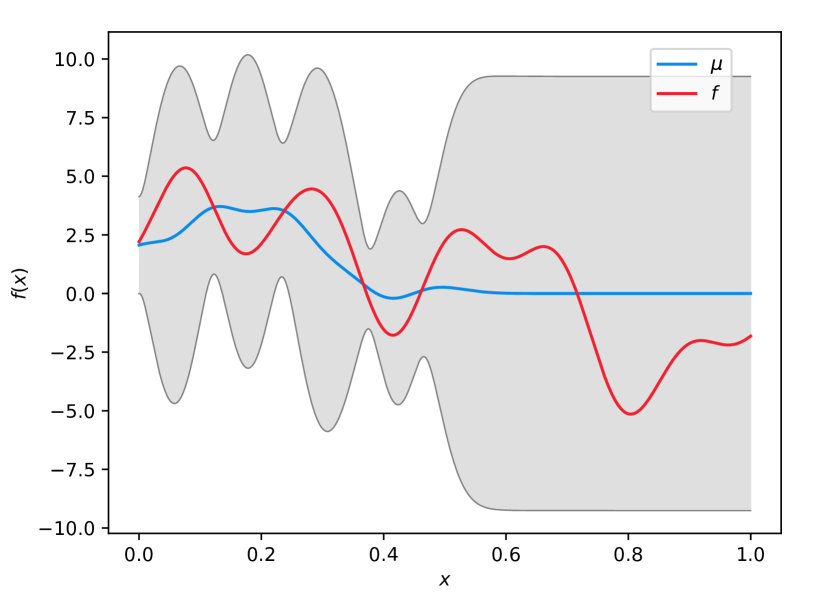
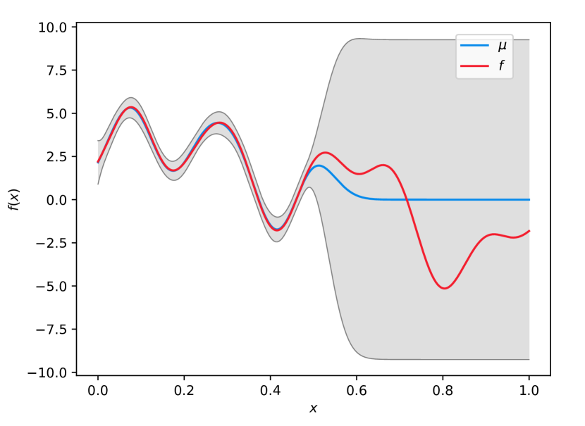
Fig.​ 2: We simulate a GP on $[0,1]\in\mathbb{R}$ using Gaussian kernel with bandwidth $\sigma^{2}\triangleq 100$. We draw $f$ from the GP and give to BKB $t\in\{6,63,215\}$ evaluations sampled uniformly in $[0,0.5]$. We plot $f$ and $\widetilde{\mu}_{t}\pm 3\widetilde{\sigma}_{t}$.

Let $m_{t}\triangleq|\mathcal{S}_{t}|$ be the size of the set $\mathcal{S}_{t}$ at step $t$. At each step, we first compute the embedding $\mathbf{z}_{t}(\mathbf{x}_{i})$ of all arms in $\mathcal{O}(Am_{t}^{2}+m_{t}^{3})$ time, which corresponds to one inversion of $\mathbf{K}_{\mathcal{S}_{t}}^{1/2}$ and the matrix-vector product specific to each arm. We then rebuild the matrix $\mathbf{V}_{t}$ from scratch using all the arms observed so far. In general, it is sufficient to use counters to record the arms pulled so far, rather than the full list of arms, so that $\mathbf{V}_{t}$ can be constructed in $\mathcal{O}(\min\{t,A\}m_{t}^{2})$ time. Then, the inverse $\mathbf{V}_{t}^{-1}$ is computed in $\mathcal{O}(m_{t}^{3})$ time. We can now efficiently compute $\widetilde{\mu}_{t}$, $\widetilde{\sigma}_{t}$, and $\widetilde{u}_{t}$ for all arms in $\mathcal{O}(Am_{t}^{2})$ time reusing the embeddings and $\mathbf{V}_{t}^{-1}$. Finally, computing all $q_{t+1,i}$s and $\mathcal{S}_{t+1}$ takes $\mathcal{O}(\min\{t+1,A\})$ time using the estimated variances $\widetilde{\sigma}_{t}^{2}$. As a result, the per-step complexity is of order $\mathcal{O}\big{(}(A+\min\{t,A\})m_{T}^{2}\big{)}$. Space-wise, we only need to store the embedded arms and $\mathbf{V}_{t}$ matrix, which takes at most $\mathcal{O}(Am_{T})$ space.
The size of $\mathcal{S}_{T}$. The size $m_{t}$ of $\mathcal{S}_{t}$ can be expressed using the $q_{t,i}$ r.v. as the sum $m_{t}\triangleq\sum_{i=1}^{t}q_{t,i}$. In order to provide a bound on the total number of inducing points, which directly determines the computational complexity of BKB, we go through three major steps.

The first is to show that w.h.p., $m_{t}$ is close to the sum $\sum_{i=1}^{t}\widetilde{p}_{t,i}=\sum_{i=1}^{t}\overline{q}\widetilde{\sigma}_{t}^{2}(\widetilde{\mathbf{x}}_{i})$, i.e., close to the sum of the probabilities we used to sample each $q_{t,i}$. However, the different $q_{t,i}$ are not independent and each $\widetilde{p}_{t,i}$ is itself a r.v. Nonetheless all $q_{t,i}$ are conditionally independent given the previous $t-1$ steps, and this is sufficient to obtain the result.

The second and a more complex step is to guarantee that the random sum $\sum_{i=1}^{t}\widetilde{\sigma}_{t}^{2}(\widetilde{\mathbf{x}}_{i})$ is close to $\sum_{i=1}^{t}\sigma_{t}^{2}(\widetilde{\mathbf{x}}_{i})$ and, at a lower level, that each individual estimate $\widetilde{\sigma}_{t}^{2}(\cdot)$ is close to $\sigma_{t}^{2}(\cdot)$. To achieve this we exploit the connection between ridge leverage scores and posterior variance $\sigma_{t}^{2}$. In particular, we show that the variance estimator $\widetilde{\sigma}_{t}^{2}(\cdot)$ used by BKB is a variation of the RLS estimator of Calandriello et al. (2017a) for RLS sampling. As a consequence, we can transfer the strong accuracy and size guarantees of RLS sampling to our optimization setting (see Appendix C).color=yellow]Add ref to appendix. Note that anchoring the probabilities to the RLS (i.e. the sum of the posterior variances) means that the size of $\mathcal{S}_{t}$ naturally follows the effective dimension of the arms pulled so far. This strikes an adaptive balance between decreasing each individual probability to avoid $\mathcal{S}_{t}$ growing too large, while at the same time automatically increasing the effective degrees of freedom of the sparse GP when necessary.

The first two steps lead to $m_{t}\approx\sum_{i=1}^{t}\sigma_{i}^{2}(\widetilde{\mathbf{x}}_{i})$, for which we need to derive a more explicit bound. In the GP analyses, this quantity is bounded using the maximal information gain $\gamma_{T}$ after $T$ rounds. For this, let $\mathbf{X}_{\mathcal{A}}\in\mathbb{R}^{A\times d}$ be the matrix with all arms as rows, $\mathcal{D}$ a subset of these rows, potentially with duplicates, and ${\mathbf{K}}_{\mathcal{D}}$ the associated kernel matrix. Then, Srinivas et al. (2010) define

$$\gamma_{T}\triangleq\max_{\mathcal{D}\subset\mathcal{A}:|\mathcal{D}|=T}\tfrac{1}{2}\operatorname*{log\,det}({\mathbf{K}}_{\mathcal{D}}/\lambda+\mathbf{I}),\vspace{-0.2\baselineskip}$$

and show that $\sum_{i=1}^{t}\sigma_{i}^{2}(\widetilde{\mathbf{x}}_{i})\leq\gamma_{t}$, and that $\gamma_{T}$ itself can be bounded for specific $\mathcal{A}$ and kernel functions, e.g., $\gamma_{T}\leq\mathcal{O}(\log(T)^{d+1})$ for Gaussian kernels. Using the equivalence between RLS and posterior variance $\sigma_{t}^{2}$, we can also relate the posterior variance $\sigma_{t}^{2}(\widetilde{\mathbf{x}}_{i})$ of the evaluated arms to the so-called GP’s effective dimension $d_{\text{\rm eff}}$ or degrees of freedom

$$\vspace{-0.3\baselineskip}d_{\text{\rm eff}}(\lambda,\widetilde{\mathbf{X}}_{T})\triangleq\sum\nolimits_{i=1}^{t}\sigma_{t}^{2}(\widetilde{\mathbf{x}}_{i})=\operatorname*{Tr}({\mathbf{K}}_{T}({\mathbf{K}}_{T}+\lambda\mathbf{I})^{-1}),\vspace{-0.1\baselineskip}$$ (5)

using the following inequality by Calandriello et al. (2017b),

$$\operatorname*{log\,det}\mathopen{}\mathclose{{}\left({\mathbf{K}}_{T}/\lambda+\mathbf{I}}\right)\leq\operatorname*{Tr}({\mathbf{K}}_{T}({\mathbf{K}}_{T}+\lambda\mathbf{I})^{-1})\mathopen{}\mathclose{{}\left(1+\log\mathopen{}\mathclose{{}\left(\tfrac{\|{\mathbf{K}}_{T}\|}{\lambda}+1}\right)}\right).$$ (6)

We use both RLS and $d_{\text{\rm eff}}$ to describe BKB’s selection. We now give the main result of this section.

Theorem 3.1.

For a desired $0<\varepsilon<1$, $0<\delta<1$, let $\alpha\triangleq(1+\varepsilon)/(1-\varepsilon)$. If we run BKB with $\overline{q}\geq 6\alpha\log(4T/\delta)/\varepsilon^{2},$ then with probability $1-\delta$, for all $t\in[T]$ and for all $\mathbf{x}\in\mathcal{A},$ we have

$$\sigma_{t}^{2}(\mathbf{x})/\alpha\leq\widetilde{\sigma}_{t}^{2}(\mathbf{x})\leq\alpha\sigma_{t}^{2}(\mathbf{x}) |\mathcal{S}_{t}|\leq 3(1+\kappa^{2}/\lambda)\alpha\overline{q}d_{\text{\rm eff}}(\lambda,\widetilde{\mathbf{X}}_{t}).$$ and

Computational complexity. We already showed that BKB’s implementation with Nyström embedding requires $\mathcal{O}(T(A+\min\{t,A\})m_{T}^{3})$ time and $\mathcal{O}(Am_{T})$ space. Combining this with Theorem 3.1 and the bound $m_{T}\leq\widetilde{\mathcal{O}}(d_{\text{\rm eff}})$, we obtain a $\widetilde{\mathcal{O}}(TAd_{\text{\rm eff}}^{2}+\min\{t,A\})d_{\text{\rm eff}}^{3})$ time complexity. Whenever $d_{\text{\rm eff}}\ll T$ and $T\ll A$, this is essentially a quadratic $\mathcal{O}(T^{2})$ runtime, a large improvement over the quartic $\mathcal{O}(T^{4})\leq\mathcal{O}(T^{3}A)$ runtime of GP-UCB.
Tuning $\overline{q}$. Note that although $\overline{q}$ must satisfy the condition of Theorem 3.1 for the result to hold, it is quite robust to uncertainty on the desired horizon $T$. In particular, the bound holds for any $\varepsilon>0$, and even if we continue updating $\mathcal{S}_{T}$ after the $T$-th step, the bound still holds by implicitly increasing the parameter $\varepsilon$. Alternatively, after the $T$-th iteration the user can suspend the algorithm, increase $\overline{q}$ to suit the new desired horizon, and rerun only the subset selection on the arms selected so far.
Avoiding variance starvation. Another important consequence of Theorem 3.1 is that BKB’s variance estimate is always close to the exact one up to a small constant factor. To the best of our knowledge, it makes BKB the first efficient and general GP algorithm that provably avoids variance starvation, which can be caused by two sources of error. The first source is the degeneracy, i.e., low-rankness of the GP approximation which causes the estimate to grow over-confident when the number of observed points grows and exceeds the degrees of freedom of the GP. BKB adaptively chooses its degrees of freedom as the size of $\mathcal{S}_{t}$ scales with the effective dimension. The second source of error arises when a point is far away from $\mathcal{S}_{t}$. Our use of a DTC variance estimator avoids under-estimation before we update the subset $\mathcal{S}_{t}$. Afterward, we can use guarantees on the quality of $\mathcal{S}_{t}$ to guarantee that we do not over-estimate the variance too much, exploiting a similar approach used to guarantee accuracy in RLS estimation. Both problems, and BKB’s accuracy, are highlighted in Figure 2 using a benchmark experiment proposed by Wang et al. (2018).
Incremental dictionary update. At each step $t$, BKB recomputes the dictionary $\mathcal{S}_{t+1}$ from scratch by sampling each of the arms pulled so far with a suitable probability $\widetilde{p}_{t+1,i}$. A more efficient variant would be to build $\mathcal{S}_{t+1}$ by adding the new point ${\mathbf{x}}_{t+1}$ with probability $\widetilde{p}_{t+1,t+1}$ and including the points in $\mathcal{S}_{t}$ with probability $\widetilde{p}_{t+1,i}/\widetilde{p}_{t,i}$. This strategy is used in the streaming setting to avoid storing all points observed so far and incrementally update the dictionary (see Calandriello et al., 2017a). Nonetheless, the stream of points, although arbitrary, is assumed to be generated independently from the dictionary itself. On the other hand, in our bandit setting, the points $\widetilde{{\mathbf{x}}}_{1},\widetilde{{\mathbf{x}}}_{2},\ldots$ are actually chosen by the learner depending on the dictionaries built over time, thus building a strong dependency between the stream of points and the dictionary itself. How to analyze such dependency and whether the accuracy of the inducing points is preserved in this case remains as an open question. Finally, notice that despite being more elegant and efficient, such incremental dictionary update would not significantly reduce the asymptotic computational complexity, since maximiming $u_{t}$, whose main cost is computing the posterior variance for each arm, would still dominate the overall runtime.

4 Regret Analysis

We are now ready to present the second main contribution of this paper, a bound on the regret achieved by BKB. To prove our result we additionally assume that the reward function $f$ has a bounded norm, i.e., $\|f\|_{\mathcal{H}}^{2}\triangleq\langle f,f\rangle<\infty$. We use an upper-bound $\|f\|_{\mathcal{H}}\leq F$ to properly tune $\widetilde{\beta}_{t}$ to the range of the rewards. If $F$ is not known in advance, standard guess-and-double techniques apply.

Theorem 4.1.

Assume $\|f\|_{\mathcal{H}}\leq F<\infty$. For any desired $0<\varepsilon<1$, $0<\delta<1$, $0<\lambda$, let $\alpha\triangleq(1+\varepsilon)/(1-\varepsilon)$ and $\overline{q}\geq 6\alpha\log(4T/\delta)/\varepsilon^{2}$. If we run BKB withcolor=yellow]What is $\xi$?

$$\widetilde{\beta}_{t}\triangleq 2\xi\sqrt{\alpha\log(\kappa^{2}t)\mathopen{}\mathclose{{}\left(\sum\nolimits_{s=1}^{t}\widetilde{\sigma}_{t}^{2}(\widetilde{\mathbf{x}}_{s})}\right)+\log(1/\delta)}+\mathopen{}\mathclose{{}\left(1+\tfrac{1}{\sqrt{1-\varepsilon}}}\right)\sqrt{\lambda}F,$$

then, with probability of at least $1-\delta$, the regret $R_{T}$ of BKB is bounded as

$$R_{T}\leq 2(2\alpha)^{3/2}\sqrt{T}\mathopen{}\mathclose{{}\left(\xi d_{\text{\rm eff}}(\lambda,\widetilde{\mathbf{X}}_{T})\log(\kappa^{2}T)+\sqrt{\lambda F^{2}d_{\text{\rm eff}}(\lambda,\widetilde{\mathbf{X}}_{T})\log(\kappa^{2}T)}+\xi\log(1/\delta)}\right).$$

Theorem 4.1 shows that BKB achieves exactly the same regret as (exact) GP-UCB up to small $\alpha$ constant and $\log(\kappa^{2}T)$ multiplicative factor. For instance, setting $\varepsilon=1/2$ results in a bound only $3\log(T)$ times larger than the one of GP-UCB. At the same time, the choice $\varepsilon=1/2$ only accounts for a constant factor $12$ in the per-step computational complexity, which is still dramatically reduced from $t^{2}A$ to $d_{\text{\rm eff}}^{2}A$. Note also that even if we send $\varepsilon$ to $0$, in the worst case we will include all arms selected so far, i.e., $\mathcal{S}_{t}=\{\widetilde{\mathbf{X}}_{t}\}$. Therefore, even in this case BKB’s runtime does not grow unbounded, but BKB transforms back into exact GP-UCB. Moreover, we show that $d_{\text{\rm eff}}(\lambda,\widetilde{\mathbf{X}}_{T})\leq\operatorname*{log\,det}({\mathbf{K}}_{T}/\lambda+\mathbf{I})$, as in Proposition B.3 in the appendix, so any bound on $\operatorname*{log\,det}({\mathbf{K}}_{T}/\lambda+\mathbf{I})$ available for GP-UCB applies directly to BKB. This means that up to an extra $\log T$ factor, we match GP-UCB’s $\widetilde{\mathcal{O}}(\log(T)^{2d})$ rate for the Gaussian kernel, $\widetilde{\mathcal{O}}(T^{\frac{1}{2}\frac{2\nu+3d^{2}}{2\nu+d^{2}}})$ rate for the Matérn kernel, and $\widetilde{\mathcal{O}}(d\sqrt{T})$ for the linear kernel. While these bounds are not minimax optimal, they closely follow the lower bounds derived in Scarlett et al. (2017). On the other hand, in the case of linear kernel (i.e., the linear bandits) we nearly match the lower bound of Dani et al. (2008).

Another interesting aspect of BKB is that computing the trade-off parameter $\widetilde{\beta}_{t}$ can be done efficiently. Previous methods bounded this quantity with a loose (deterministic) upper bound, e.g., $\mathcal{O}(\log(T)^{d})$ for Gaussian kernels, to avoid the large cost of computing $\operatorname*{log\,det}({\mathbf{K}}_{T}/\lambda+\mathbf{I})$. In our $\widetilde{\beta}_{t}$, we bound the $\operatorname*{log\,det}$ by $d_{\text{\rm eff}}$, which is then bounded by $\sum\nolimits_{s=1}^{t}\widetilde{\sigma}_{t}^{2}(\mathbf{x}_{s})$, see Thm. 3.1, where all $\widetilde{\sigma}_{t}^{2}$s are already efficiently computed at each step. While this is up to $\log t$ larger than the exact $\operatorname*{log\,det}$, it is data adaptive and much smaller than the known worst case upper bounds.

It it crucial, that our regret guarantee is achieved without requiring an increasing accuracy in our approximation. One would expect that to obtain a sublinear regret the error induced by the approximation should decrease as $1/T$. Instead, in BKB, the constants $\varepsilon$ and $\lambda$ that govern the accuracy level are fixed and thus it is not possible to guarantee that $\widetilde{\mu}_{t}$ will ever get close to $\mu_{t}$ everywhere. Adaptivity is the key: we can afford the same approximation level at every step because accuracy is actually increased only on a specific part of the arm set. For example, if a suboptimal arm is selected too often due to bad approximation, it will be eventually included in $\mathcal{S}_{t}$. After the inclusion, the approximation accuracy in the region of the suboptimal arm increases, and it would not be selected anymore. As the set of inducing points is updated fast enough, the impact of inaccurate approximations is limited over time, thus preventing large regret to accumulate. Note that this is a significant divergence from existing results. In particular approximation bounds that are uniformly accurate for all $\mathbf{x}_{i}\in\mathcal{A}$, such as those obtained with quadrature FF (Mutný and Krause, 2018), rely on packing arguments. Due to the nature of packing, this usually causes the runtime or regret to scale exponentially with the input dimension $d$, and requires kernel $k$ to have a specific structure, e.g., to be stationary. Our new analysis avoids both of these problems.

Finally, we point out that the adaptivity of BKB allows drawing an interesting connection between learning and computational complexity. In fact, both the regret and the computation of BKB scale with the log-determinant and effective dimension of ${\mathbf{K}}_{T}$, which is related to the effective dimension of the sequence of arms selected over time. As a result, if the problem is difficult from a learning point of view (i.e., the regret is large because of large log-determinant), then BKB automatically adapts the set $\mathcal{S}_{t}$ by including many more inducing points to guarantee the level of accuracy needed to solve the problem. Conversely, if the problem is simple (i.e., small regret), then BKB can greatly reduce the size of $\mathcal{S}_{t}$ and achieve the derived level of accuracy.

4.1 Proof sketch

We build on the GP-UCB analysis of  Chowdhury and Gopalan (2017). Their analysis relies on a confidence interval formulation of GP-UCB that is more conveniently expressed using an explicit feature-based representation of the GP. For any GP with covariance $k$, there is a corresponding RKHS $\mathcal{H}$ with $k$ as its kernel function. Furthermore, any kernel function $k$ is associated to a non-linear feature map $\boldsymbol{\phi}(\cdot):\mathbb{R}^{d}\rightarrow\mathcal{H}$ such that $k(\mathbf{x},\mathbf{x}^{\prime})=\boldsymbol{\phi}(\mathbf{x}^{\prime})^{\mathsf{\scriptscriptstyle T}}\boldsymbol{\phi}(\mathbf{x}^{\prime})$. As a result, any reward function $f\in\mathcal{H}$ can be written as $f(\mathbf{x})=\boldsymbol{\phi}(\mathbf{x})^{\mathsf{\scriptscriptstyle T}}\mathbf{w}_{\star}$, where $\mathbf{w}_{\star}\in\mathcal{H}$.

Confidence-interval view of GP-UCB.

Let $\boldsymbol{\Phi}(\mathbf{X}_{t})\triangleq[\boldsymbol{\phi}(\mathbf{x}_{1}),\dots,\boldsymbol{\phi}(\mathbf{x}_{t})]^{\mathsf{\scriptscriptstyle T}}$ be the matrix $\mathbf{X}_{t}$ after the application of $\boldsymbol{\phi}(\cdot)$ to each row. We can then define the regularized design matrix as $\mathbf{A}_{t}\triangleq\boldsymbol{\Phi}(\mathbf{X}_{t})^{\mathsf{\scriptscriptstyle T}}\boldsymbol{\Phi}(\mathbf{X}_{t})+\lambda\mathbf{I}$, and then compute the regularized least-squares estimate as

$$\widehat{\mathbf{w}}_{t} \triangleq\operatorname*{arg\,min}_{\mathbf{w}\in\mathcal{H}}\sum\nolimits_{i=1}^{t}(y_{i}-\boldsymbol{\phi}(\mathbf{x}_{i})^{\mathsf{\scriptscriptstyle T}}\mathbf{w})^{2}+\lambda\|\mathbf{w}\|_{2}^{2}=\mathbf{A}_{t}^{-1}\boldsymbol{\Phi}(\mathbf{X}_{t})^{\mathsf{\scriptscriptstyle T}}\mathbf{y}_{t}.$$

We define the confidence interval $C_{t}$ as the ellipsoid induced by $\mathbf{A}_{t}$ with center $\widehat{\mathbf{w}}_{t}$ and radius $\beta_{t}$

$$C_{t} \triangleq\mathopen{}\mathclose{{}\left\{\mathbf{w}:\|\mathbf{w}-\widehat{\mathbf{w}}_{t}\|_{\mathbf{A}_{t}}\leq\beta_{t}}\right\},\quad\quad\beta_{t}\triangleq\lambda^{1/2}F+R\sqrt{2(\operatorname*{log\,det}(\mathbf{A}_{t}/\lambda)+\log(1/\delta)},$$ (7)

where the radius $\beta_{t}$ is such that $\mathbf{w}_{\star}\in C_{t}$ w.h.p. ​(Chowdhury and Gopalan, 2017). Finally, using Lagrange multipliers we reformulate the GP-UCB scores as

$$u_{t}(\mathbf{x}_{i}) =\max_{\mathbf{w}\in C_{t}}\boldsymbol{\phi}(\mathbf{x}_{i})^{\mathsf{\scriptscriptstyle T}}\mathbf{w}=\overbracket{\boldsymbol{\phi}(\mathbf{x}_{i})^{\mathsf{\scriptscriptstyle T}}\widehat{\mathbf{w}}_{t}}^{\mu_{t}(\mathbf{x}_{i})}+\beta_{t}\overbracket{\sqrt{\boldsymbol{\phi}(\mathbf{x}_{i})^{\mathsf{\scriptscriptstyle T}}\mathbf{A}_{t}^{-1}\boldsymbol{\phi}(\mathbf{x}_{i})}.}^{\sigma_{t}(\mathbf{x}_{i})}$$ (8)

Approximating the confidence ellipsoid. Consider subset of arm $\mathcal{S}_{t}=\{\mathbf{x}_{i}\}_{i=1}^{m}$ chosen by BKB at each step and denote by $\mathbf{X}_{\mathcal{S}_{t}}\in\mathbb{R}^{m\times d}$ the matrix with all arms in $\mathcal{S}_{t}$ as rows. Let $\widetilde{\mathcal{H}}_{t}\triangleq\operatorname*{Im}(\boldsymbol{\Phi}(\mathbf{X}_{\mathcal{S}_{t}}))$ be the smaller $m$-rank RKHS spanned by $\boldsymbol{\Phi}(\mathbf{X}_{\mathcal{S}_{t}});$ and by $\mathbf{P}_{t}$ the symmetric orthogonal projection operator on $\widetilde{\mathcal{H}}_{t}$. We then define an approximate feature map $\widetilde{\boldsymbol{\phi}}_{t}(\cdot)\triangleq\mathbf{P}_{t}\boldsymbol{\phi}(\cdot):\mathbb{R}^{d}\rightarrow\widetilde{\mathcal{H}}_{t}$ and associated approximations of $\mathbf{A}_{t}$ and $\widehat{\mathbf{w}}_{t}$ as

$$\widetilde{\mathbf{A}}_{t} \triangleq\widetilde{\boldsymbol{\Phi}}_{t}(\mathbf{X}_{t})^{\mathsf{\scriptscriptstyle T}}\widetilde{\boldsymbol{\Phi}}_{t}(\mathbf{X}_{t})+\lambda\mathbf{I},$$ (9)

$$\widetilde{\mathbf{w}}_{t} \triangleq\operatorname*{arg\,min}_{\mathbf{w}\in\mathcal{H}}\sum_{i=1}^{t}(y_{i}-\widetilde{\boldsymbol{\phi}}(\mathbf{x}_{i})^{\mathsf{\scriptscriptstyle T}}\mathbf{w})^{2}+\lambda\|\mathbf{w}\|_{2}^{2}=\widetilde{\mathbf{A}}_{t}^{-1}\widetilde{\boldsymbol{\Phi}}_{t}(\mathbf{X}_{t})^{\mathsf{\scriptscriptstyle T}}\mathbf{y}_{t}.$$ (10)

This leads to an approximate confidence ellipsoid $\widetilde{C}_{t}\triangleq\big{\{}\mathbf{w}:\|\mathbf{w}-\widetilde{\mathbf{w}}_{t}\|_{\widetilde{\mathbf{A}}_{t}}\leq\widetilde{\beta}_{t}\big{\}}.$ A subtle element in these definitions is that while $\widetilde{\boldsymbol{\Phi}}_{t}(\mathbf{X}_{t})^{\mathsf{\scriptscriptstyle T}}\widetilde{\boldsymbol{\Phi}}_{t}(\mathbf{X}_{t})$ and $\widetilde{\mathbf{w}}_{t}$ are now restricted to $\widetilde{\mathcal{H}}_{t}$, the identity operator $\lambda\mathbf{I}$ in the regularization of $\widetilde{\mathbf{A}}_{t}$ still acts over the whole $\mathcal{H}$, and therefore $\widetilde{\mathbf{A}}_{t}$ does not belong to $\widetilde{\mathcal{H}}_{t}$ and remains full-rank and invertible. This immediately leads to the usage of $k(\mathbf{x}_{i},\mathbf{x}_{i})$ in the definition of $\widetilde{\sigma}$ in Eq. 3.1, instead of the its approximate version using the Nyström embedding.

Bounding the regret. To find an appropriate $\widetilde{\beta}_{t}$ we follow an approach similar to the one of Abbasi-Yadkori et al. (2011). Exploiting the relationship $y_{t}=\widetilde{\boldsymbol{\phi}}(\widetilde{\mathbf{x}}_{t})^{\mathsf{\scriptscriptstyle T}}\mathbf{w}_{\star}+\eta_{t}$, we bound

$$\|\mathbf{w}_{\star}-\widetilde{\mathbf{w}}_{t}\|^{2}_{\widetilde{\mathbf{A}}_{t}}\leq\overbracket{\lambda^{1/2}\|\mathbf{w}_{\star}\|}^{(a)}+\overbracket{\|\widetilde{\boldsymbol{\Phi}}_{t}(\mathbf{X}_{t})\boldsymbol{\eta}_{t}\|_{\widetilde{\mathbf{A}}_{t}^{-1}}}^{(b)}+\overbracket{\|\boldsymbol{\Phi}(\mathbf{X}_{t})^{\mathsf{\scriptscriptstyle T}}\|_{\mathbf{I}-\mathbf{P}_{t}}\cdot\|\mathbf{w}_{\star}\|}^{(c)}\!.$$

Both $(a)$ and $(b)$ are present in GP-UCB and OFUL’s analysis. The first term $(a)$ is due to the bias introduced in the least-square estimator $\widetilde{\mathbf{w}}_{t}$ by the regularization $\lambda$. Then, term $(b)$ is due to the noise in the reward observations. Note that the same term $(b)$ appears in GP-UCB’s analysis as $\|\boldsymbol{\Phi}(\mathbf{X}_{t})\boldsymbol{\eta}_{t}\|_{\mathbf{A}_{t}^{-1}}$ and it is bounded by $\operatorname*{log\,det}(\mathbf{A}_{t}/\lambda)$ using self-normalizing concentration inequalities Chowdhury and Gopalan (2017). However, our $\|\widetilde{\boldsymbol{\Phi}}_{t}(\mathbf{X}_{t})\boldsymbol{\eta}_{t}\|_{\widetilde{\mathbf{A}}_{t}^{-1}}$ is a more complex object, since the projection $\mathbf{P}_{t}$ contained in $\widetilde{\boldsymbol{\Phi}}_{t}(\mathbf{X}_{t})\triangleq\mathbf{P}_{t}\boldsymbol{\Phi}(\mathbf{X}_{t})$ depends on the whole process up to time time $t$, and therefore $\widetilde{\boldsymbol{\Phi}}_{t}(\mathbf{X}_{t})$ also depends on the whole process, losing its martingale structure. To avoid this, we use Sylvester’s identity and the projection operator $\mathbf{P}_{t}$ to bound

$$\operatorname*{log\,det}(\widetilde{\mathbf{A}}_{t}/\lambda)=\operatorname*{log\,det}\mathopen{}\mathclose{{}\left(\tfrac{\boldsymbol{\Phi}(\mathbf{X}_{t})\mathbf{P}_{t}\boldsymbol{\Phi}(\mathbf{X}_{t})^{\mathsf{\scriptscriptstyle T}}}{\lambda}+\mathbf{I}}\right)\leq\operatorname*{log\,det}\mathopen{}\mathclose{{}\left(\tfrac{\boldsymbol{\Phi}(\mathbf{X}_{t})\boldsymbol{\Phi}(\mathbf{X}_{t})^{\mathsf{\scriptscriptstyle T}}}{\lambda}+\mathbf{I}}\right)=\operatorname*{log\,det}(\mathbf{A}_{t}/\lambda).\vspace{-.35\baselineskip}$$

In other words, restricting the problem to $\widetilde{\mathcal{H}}_{t}$ acts as a regularization and reduces the variance of the martingale. Unfortunately, $\operatorname*{log\,det}(\mathbf{A}_{t}/\lambda)$ is too expensive to compute, so we first bound it with $d_{\text{\rm eff}}(\lambda,\widetilde{\mathbf{X}}_{t})\log(\kappa^{2}t)$, and then we bound $d_{\text{\rm eff}}(\lambda,\widetilde{\mathbf{X}}_{t})\leq\alpha\sum\nolimits_{s=1}^{t}\widetilde{\sigma}_{t}^{2}(\mathbf{x}_{s}),$ Theorem 3.1, which can be computed efficiently. Finally, a new bias term $(c)$ appears. Combining Theorem 3.1 with the results of Calandriello and Rosasco (2018) for projection $\mathbf{P}_{t}$ obtained using RLSs sampling, we show that

$$\mathbf{I}-\mathbf{P}\preceq\lambda\mathbf{A}_{t}^{-1}/(1-\varepsilon).$$

The combination of $(a)$, $(b)$, and $(c)$ leads to the definition of $\widetilde{\beta}_{t}$ and the final regret bound as $R_{T}\leq\sqrt{\widetilde{\beta}_{T}}\sqrt{\sum\nolimits_{t=1}^{T}\boldsymbol{\phi}(\mathbf{x}_{t})^{\mathsf{\scriptscriptstyle T}}\widetilde{\mathbf{A}}_{t}^{-1}\boldsymbol{\phi}(\mathbf{x}_{t})}$. To conclude the proof, we bound $\sum\nolimits_{t=1}^{T}\boldsymbol{\phi}(\mathbf{x}_{t})^{\mathsf{\scriptscriptstyle T}}\widetilde{\mathbf{A}}_{t}^{-1}\boldsymbol{\phi}(\mathbf{x}_{t})$ with the following corollary of Theorem 3.1.

Corollary 4.2.

Under the same conditions as Theorem 4.1, for all $t\in T$, we have $\mathbf{A}_{t}/\alpha\preceq\widetilde{\mathbf{A}}_{t}\preceq\alpha\mathbf{A}_{t}.$

Remarks. The novel bound $\|\boldsymbol{\Phi}(\mathbf{X}_{t})^{\mathsf{\scriptscriptstyle T}}\|_{\mathbf{I}-\mathbf{P}_{t}}\leq\tfrac{\lambda}{1-\varepsilon}\|\boldsymbol{\Phi}(\mathbf{X}_{t})^{\mathsf{\scriptscriptstyle T}}\|_{\mathbf{A}_{t}^{-1}}$ has a crucial role in controlling the bias due to the projection $\mathbf{P}_{t}$. Note that the second term measures the error with the same metric $\mathbf{A}_{t}^{-1}$ used by the variance martingale. In other words, the bias introduced by BKB’s approximation can be seen as a self-normalizing bias. It is larger along directions that have been sampled less frequently, and smaller along directions correlated with arms selected often (e.g., the optimal arm).
Our analysis bears some similarity with the one recently and independently developed by Kuzborskij et al. (2019). Nonetheless, our proof improves their result along two dimensions. First, we consider the more general (and challenging) GP optimization setting. Second, we do not fix the rank of our approximation in advance. While their analysis also exploits a self-normalized bias argument, this applies only to the $k$ largest components. If the problem has an effective dimension larger than $k$, their radius and regret becomes essentially linear. In BKB we use our adaptive sampling scheme to include all necessary directions and to achieve the same regret rate as exact GP-UCB.

5 Discussion

As the prior work in Bayesian optimization is vast, we do not compare to alternative GP acquisition functions, such as GP-EI or GP-PI, and only focus on approximation techniques with theoretical guarantees. Similarly, we exclude scalable variational inference based methods, even when their approximate posterior is provably accurate such as pF-DTC (Huggins et al., 2019), since they only provide guarantees for GP regression and not for the more difficult optimization setting. We also do not discuss SupKernelUCB (Valko et al., 2013), which has a tighter analysis than GP-UCB, since the algorithm does not work well in practice.

Infinite arm sets. Looking at the proof of Theorem 3.1, the guarantees on $\widetilde{u}_{t}$ hold for any $\mathcal{H}$, and in Theorem 4.1, we only require that the maximum $\widetilde{\mathbf{x}}_{t+1}\triangleq\operatorname*{arg\,max}_{\mathbf{x}\in\mathcal{A}}\max_{\mathbf{w}\in\widetilde{C}_{t}}\boldsymbol{\phi}(\mathbf{x})^{\mathsf{\scriptscriptstyle T}}\mathbf{w}$ is returned. Therefore, the accuracy and regret guarantees also hold also for an infinite set of arms $\mathcal{A}$. However, the search over $\mathcal{A}$ can be difficult. In the general case, maximization of a GP posterior is an NP-hard problem, with algorithms that often scale exponentially with the input dimension $d$ and are not practical. We treated the easier case of finite sets, where enumeration is sufficient. Note that this automatically introduces an $\Omega(A)$ runtime dependency, which could be removed if the user provides an efficient method to solve the maximization problem on a specific infinite set $\mathcal{A}$. As an example, Mutný and Krause (2018) prove that a GP posterior approximated using QFF can be optimized efficiently in low dimensions and we expect similar results hold for BKB and low effective dimension. Finally, note that recomputing a new set $\mathcal{S}_{t}$ still requires $\min\{A,t\}d_{\text{\rm eff}}^{2}$ at each step. As discussed at the end of Section 3, this is a bottleneck in BKB due to the non-incremental dictionary sampling and independent from the arm selection. How to address it remains an open question.
Linear bandit with matrix sketching. Our analysis is related to the ones of CBRAP  (Yu et al., 2017) and SOFUL (Kuzborskij et al., 2019). CBRAP uses Gaussian projections to embed all arms in a lower dimensional space for efficiency. Unfortunately their approach must either use an embedded space at least $\Omega(T)$ large, which in most cases would be even slower than exact OFUL, or it incurs linear regret w.h.p. Another approach for Euclidean spaces based on matrix approximation is SOFUL, introduced by Kuzborskij et al. (2019). It uses Frequent Direction (Ghashami et al., 2016), a method similar to incremental PCA, to embed the arms into $\mathbb{R}^{m}$, where $m$ is fixed in advance. To compare, we distinguish between SOFUL-UCB and SOFUL-TS, a variant based on Thompson sampling. SOFUL-UCB achieves a $\widetilde{\mathcal{O}}(TAm^{2})$ runtime and $\widetilde{\mathcal{O}}((1+\varepsilon_{m})^{3/2}(d+m)\sqrt{T})$ regret, where $\varepsilon_{m}$ is the sum of the $d-m$ smallest eigenvalues of $\mathbf{A}_{T}$. However, notice that if the tail do not decrease quickly, this algorithm also suffers linear regret and no adaptive way to tune $m$ is known. On the same task BKB achieves a $\widetilde{\mathcal{O}}(d\sqrt{T})$ regret, since it adaptively chooses the size of the embedding. Computationally, directly instantiating BKB to use a linear kernel would achieve a $\widetilde{\mathcal{O}}(TAm_{t}^{2})$ runtime, matching Kuzborskij et al. (2019)’s. Compared to SOFUL-TS, BKB achieves better regret, but is potentially slower. Since Thompson sampling does not need to compute all confidence intervals, but solves a simpler optimization problem, SOFUL-TS requires only $\widetilde{\mathcal{O}}(TAm)$ time against BKB’s $\widetilde{\mathcal{O}}(TAm_{t}^{2})$. It is unknown if a variant of BKB can match this complexity.

Approximate GP with RFF. Traditionally, RFF approaches have been popular to transform GP optimization in a finite-dimensional problem and allow for scalability. Unfortunately GP-UCB with traditional RFF is not low-regret, as RFF are well known to suffer from variance starvation (Wang et al., 2018) and unfeasibly large RFF embeddings would be necessary to prevent it. Recently, Mutný and Krause (2018) proposed an alternative approach based on QFF, a specialized approach to random features for stationary kernels. They achieve the same regret rate as GP-UCB and BKB, with a near-optimal $\mathcal{O}(TA\log(T)^{d+1})$ runtime. Moreover they present an additional variations based on Thompson sampling whose posterior can be exactly maximized in polynomial time if the input data is low dimensional or the covariance $k$ additive, while it is still an open question how to efficiently maximize BKB’s UCB $\widetilde{u}_{t}$ for infinite $\mathcal{A}$. However QFF based approaches apply to stationary kernel only, and require to $\varepsilon$-cover $\mathcal{A}$, hence they cannot escape an exponential dependency on the dimensionality $d$. Conversely BKB can be applied to any kernel function, and while not specifically designed for this task it also achieve a close $\widetilde{\mathcal{O}}(TA\log(T)^{3(d+1)})$ runtime. Moreover, in practice the size of $\mathcal{S}_{T}$ is less than exponential in $d$.color=yellow]How does it compare to them? Done, Daniele

Acknowledgements   This material is based upon work supported by the Center for Brains, Minds and Machines (CBMM), funded by NSF STC award CCF-1231216. L. R. acknowledges the financial support of the AFOSR projects FA9550-17-1-0390 and BAA-AFRL-AFOSR-2016-0007 (European Office of Aerospace Research and Development), and the EU H2020-MSCA-RISE project NoMADS - DLV-777826. The research presented was also supported by European CHIST-ERA project DELTA, French Ministry of Higher Education and Research, Nord-Pas-de-Calais Regional Council, Inria and Otto-von-Guericke-Universität Magdeburg associated-team north-European project Allocate, and French National Research Agency project BoB (n.ANR-16-CE23-0003). This research has also benefited from the support of the FMJH Program PGMO and from the support to this program from Criteo.

Appendix A Relaxing assumptions

In our derivations, we make several assumptions. While some are necessary, others can be relaxed.

Assumptions on the noise. Throughout the paper, we assume that the noise $\eta_{t}$ is i.i.d. Gaussian. Since Chowdhury and Gopalan’s results hold for any $\xi$-sub-Gussian noise that is measurable based with respect to the prior observations, this assumption can be easily relaxed. color=citrine, inline]adaptation to noise - if there is no noise, we can learn exponentially fast (for simple regret and therefore bounded cumulative one) https://www.icml.cc/2012/papers/853.pdf and we can adapt to it: https://arxiv.org/abs/1810.00997

Assumptions on the arms. So far we considered a set of arms that is $(a)$ in $\mathbb{R}^{d}$, $(b)$ fixed for all $t$, and $(c)$ finite. Relaxing $(a)$ is easy, since we do not make any assumption beyond boundedness on the kernel function $k$ and there are many bounded kernel function for non-Euclidean spaces, e.g., strings or graphs. Relaxing $(b)$ is trivial, we just need to embed the changing arm sets as they are provided, and store and re-embed previously selected arms as necessary. The per-step time complexity will now depend on the size of the set of arms available at each step. Relaxing $(c)$ is straightforward from a theoretical perspective, but has varying computational consequences. In particular, looking at the proof of Theorem 3.1, the guarantees on $\widetilde{u}_{t}$ hold for all $\mathcal{H}$ and in Theorem 4.1, we only require that the maximum $\widetilde{\mathbf{x}}_{t+1}\triangleq\operatorname*{arg\,max}_{\mathbf{x}\in\mathcal{A}}\max_{\mathbf{w}\in\widetilde{C}_{t}}\boldsymbol{\phi}(\mathbf{x})^{\mathsf{\scriptscriptstyle T}}\mathbf{w}$ is returned. Therefore, at least from the regret point of view, everything holds also for infinite $\mathcal{A}$. However, while the inner maximization over $\widetilde{C}_{t}$ can be solved in closed form for a fixed $\mathbf{x}$, the same cannot be said of the search over $\mathcal{A}$. If the designer can provide an efficient method to solve the maximization problem on an infinite $\mathcal{A}$, e.g., linear bandit optimization over compact subsets or $\mathbb{R}^{d}$, then all BKB guarantees apply.

Appendix B Properties of the posterior variance

For simplicity and completeness we provide known statements regarding the posterior variance $\sigma_{t}^{2}(\cdot)$. While most of these hold for generic RLS, we will adapt them to our notation.

Proposition B.1 (Calandriello et al., 2017a).

For the posterior variance, we have that

$$\frac{1}{\kappa^{2}/\lambda+1}\sigma_{t-1}^{2}(\widetilde{\mathbf{x}}_{t})\leq\frac{1}{\sigma_{t-1}^{2}(\widetilde{\mathbf{x}}_{t})+1}\sigma_{t-1}^{2}(\widetilde{\mathbf{x}}_{t})\leq\sigma_{t}^{2}(\widetilde{\mathbf{x}}_{t})\leq\sigma_{t-1}^{2}(\widetilde{\mathbf{x}}_{t}).$$

Proof B.2.

The leftmost inequality follows from $\kappa^{2}/\lambda\geq\sigma_{0}^{2}(x)$ and $\sigma^{2}_{a}(x)\geq\sigma^{2}_{b}(x),\forall a\leq b$, the others are are by Calandriello et al., 2017a.

Proposition B.3 (Hazan et al., 2006; Calandriello et al., 2017b).

The effective dimension $d_{\text{\rm eff}}(\lambda,\widetilde{\mathbf{X}}_{T})$ is upperbounded as

$$d_{\text{\rm eff}}(\lambda,\widetilde{\mathbf{X}}_{T}) \triangleq\operatorname*{Tr}({\mathbf{K}}_{T}({\mathbf{K}}_{T}+\lambda\mathbf{I})^{-1})=\sum\nolimits_{t=1}^{T}\sigma_{T}^{2}(\widetilde{\mathbf{x}}_{t})$$

$$\stackrel{{\scriptstyle(1)}}{{\leq}}\sum\nolimits_{t=1}^{T}\sigma_{t}^{2}(\widetilde{\mathbf{x}}_{t})$$

$$\stackrel{{\scriptstyle(2)}}{{\leq}}\operatorname*{log\,det}\mathopen{}\mathclose{{}\left({\mathbf{K}}_{T}/\lambda+\mathbf{I}}\right)$$

$$\stackrel{{\scriptstyle(3)}}{{\leq}}\operatorname*{Tr}({\mathbf{K}}_{T}({\mathbf{K}}_{T}+\lambda\mathbf{I})^{-1})\mathopen{}\mathclose{{}\left(1+\log\mathopen{}\mathclose{{}\left(\tfrac{\|{\mathbf{K}}_{T}\|}{\lambda}+1}\right)}\right).$$

Proof B.4.

Inequality $(1)$ is due to Proposition B.1, inequality $(2)$ is due to Hazan et al. (2006), and Inequality $(3)$ is due to Calandriello et al. (2017b).

Appendix C Proof of Theorem 3.1

Let $B_{t}$ be the unfavorable event where the guarantees of Theorem 3.1 do not hold. Our goal is to prove that $B_{t}$ happens at most with probability $\delta$ uniformly for all $t\in[T]$.

C.1 Notation

In the following we refer to $\boldsymbol{\Phi}(\widetilde{\mathbf{X}}_{t})$ as $\boldsymbol{\Phi}_{t}$, $\widetilde{\boldsymbol{\Phi}}(\widetilde{\mathbf{X}}_{t})$ as $\widetilde{\boldsymbol{\Phi}}_{t}$ and $\boldsymbol{\phi}(\widetilde{\mathbf{x}}_{t})$ as $\boldsymbol{\phi}_{t}$. When the subscript is clear from the context, we omit it. Since we leverage several results of Calandriello et al. (2017b), we start with some additional notation.

First we extend our notation for the subset $\mathcal{S}_{t}$ to include a possible reweighing of the inducing points. We denote with $\mathcal{S}_{t}\triangleq\{(\boldsymbol{\phi}_{j},s_{j})\}_{j=1}^{m_{t}},$ a weighted subset, i.e., a weighted dictionary, of columns from $\boldsymbol{\Phi}_{t}$, with positive weights $s_{j}>0$ that must be appropriately chosen. Now, denote with $i_{j}\in[t]$, the index of the sample $\boldsymbol{\phi}_{j}$ as a column in $\boldsymbol{\Phi}_{t}$. Using a standard approach (Alaoui and Mahoney, 2015), we choose $s_{j}\triangleq 1/\sqrt{\widetilde{p}_{t,i_{j}}}$, where $\widetilde{p}_{t,i}\triangleq\overline{q}\widetilde{\sigma}_{t-1}^{2}(\widetilde{\mathbf{x}}_{i})$ is the probability used by Figure 1 when sampling $\boldsymbol{\phi}_{i_{j}}$ from $\boldsymbol{\Phi}_{t}$.

Let ${\mathbf{S}}_{t}\in\mathbb{R}^{t\times t}$ be the diagonal matrix with $q_{t,i}/\sqrt{\widetilde{p}_{t,i}}$ on the diagonal, where $q_{t,i}$ are the $\{0,1\}$ random variables selected by Figure 1. Then, we can see that

$$\sum_{j=1}^{m_{t}}\frac{1}{\widetilde{p}_{t,i_{j}}}\boldsymbol{\phi}_{i_{j}}\boldsymbol{\phi}_{i_{j}}^{\mathsf{\scriptscriptstyle T}}=\sum_{i=1}^{t}\frac{q_{t,i}}{\widetilde{p}_{t,i}}\boldsymbol{\phi}_{i}\boldsymbol{\phi}_{i}^{\mathsf{\scriptscriptstyle T}}=\boldsymbol{\Phi}_{t}{\mathbf{S}}_{t}{\mathbf{S}}_{t}^{\mathsf{\scriptscriptstyle T}}\boldsymbol{\Phi}_{t}^{\mathsf{\scriptscriptstyle T}}.$$ (11)

Calandriello et al. (2017a) define $\mathcal{S}_{t}$ to be an $\varepsilon$-accurate dictionary of $\boldsymbol{\Phi}_{t}$ if it satisfies

$$(1-\varepsilon)\boldsymbol{\Phi}_{t}\boldsymbol{\Phi}_{t}^{\mathsf{\scriptscriptstyle T}}-\varepsilon\lambda\mathbf{I}\preceq\boldsymbol{\Phi}_{t}{\mathbf{S}}_{t}{\mathbf{S}}_{t}^{\mathsf{\scriptscriptstyle T}}\boldsymbol{\Phi}_{t}^{\mathsf{\scriptscriptstyle T}}\preceq(1+\varepsilon)\boldsymbol{\Phi}_{t}\boldsymbol{\Phi}_{t}^{\mathsf{\scriptscriptstyle T}}+\varepsilon\lambda\mathbf{I}.$$ (12)

color=citrine]missing ref We can also now fully define the projection operator at time $t$ (see Section 4.1 for more details) as

$$\mathbf{P}_{t}\triangleq\boldsymbol{\Phi}_{t}{\mathbf{S}}_{t}({\mathbf{S}}_{t}^{\mathsf{\scriptscriptstyle T}}\boldsymbol{\Phi}_{t}^{\mathsf{\scriptscriptstyle T}}\boldsymbol{\Phi}_{t}{\mathbf{S}}_{t})^{+}{\mathbf{S}}_{t}^{\mathsf{\scriptscriptstyle T}}\boldsymbol{\Phi}_{t}^{\mathsf{\scriptscriptstyle T}},$$

which is the projection matrix spanned by the dictionary.

C.2 Event decomposition

We decompose Theorem 3.1 into an accuracy part, i.e., $\mathcal{S}_{t}$ must induce accurate $\widetilde{\sigma}_{t}$, and an efficiency part, i.e., $m_{t}\leq d_{\text{\rm eff}}(t)$. We also the accuracy of $\widetilde{\sigma}_{t}$ to the definition of $\varepsilon$-accuracy.

Lemma C.1.

Let $\alpha\triangleq\frac{1+\varepsilon}{1-\varepsilon}$. If $\mathcal{S}_{t}$ is $\varepsilon$-accurate w.r.t. $\boldsymbol{\Phi}_{t}$, then

$$\mathbf{A}_{t}/\alpha\preceq\widetilde{\mathbf{A}}_{t}\preceq\alpha\mathbf{A}_{t}\quad\text{and}\quad\sigma_{t}^{2}(\mathbf{x})/\alpha\leq\min\mathopen{}\mathclose{{}\left\{\widetilde{\sigma}_{t}^{2}(\mathbf{x}),1}\right\}\leq\alpha\sigma_{t}^{2}(\mathbf{x})\;\text{\ for all\ }\mathbf{x}\in\mathcal{A}.$$

Proof C.2.

Inverting the bound in Equation 12 and using the fact that $\mathbf{P}_{t}\boldsymbol{\Phi}_{t}{\mathbf{S}}_{t}=\boldsymbol{\Phi}_{t}{\mathbf{S}}_{t},$ we get

$$\mathbf{P}_{t}\boldsymbol{\Phi}_{t}\boldsymbol{\Phi}_{t}^{\mathsf{\scriptscriptstyle T}}\mathbf{P}_{t} \preceq\frac{1}{1-\varepsilon}(\mathbf{P}_{t}\boldsymbol{\Phi}_{t}{\mathbf{S}}_{t}{\mathbf{S}}_{t}^{\mathsf{\scriptscriptstyle T}}\boldsymbol{\Phi}_{t}^{\mathsf{\scriptscriptstyle T}}\mathbf{P}_{t}+\varepsilon\lambda\mathbf{P}_{t})\preceq\frac{1}{1-\varepsilon}(\boldsymbol{\Phi}_{t}{\mathbf{S}}_{t}{\mathbf{S}}_{t}^{\mathsf{\scriptscriptstyle T}}\boldsymbol{\Phi}_{t}^{\mathsf{\scriptscriptstyle T}}+\varepsilon\lambda\mathbf{P}_{t})$$

$$\preceq\frac{1}{1-\varepsilon}((1+\varepsilon)\boldsymbol{\Phi}_{t}\boldsymbol{\Phi}_{t}^{\mathsf{\scriptscriptstyle T}}+\varepsilon\lambda\mathbf{I}+\varepsilon\lambda\mathbf{P}_{t})\preceq\frac{1+\varepsilon}{1-\varepsilon}\mathopen{}\mathclose{{}\left(\boldsymbol{\Phi}_{t}\boldsymbol{\Phi}_{t}^{\mathsf{\scriptscriptstyle T}}+\frac{2\varepsilon}{1+\varepsilon}\lambda\mathbf{I}}\right).$$

Repeating the same process for the other side, we obtain

$$\frac{1-\varepsilon}{1+\varepsilon}\mathopen{}\mathclose{{}\left(\boldsymbol{\Phi}_{t}\boldsymbol{\Phi}_{t}^{\mathsf{\scriptscriptstyle T}}-\frac{2\varepsilon}{1-\varepsilon}\lambda\mathbf{I}}\right)\preceq\mathbf{P}_{t}\boldsymbol{\Phi}_{t}\boldsymbol{\Phi}_{t}^{\mathsf{\scriptscriptstyle T}}\mathbf{P}_{t}\preceq\frac{1+\varepsilon}{1-\varepsilon}\mathopen{}\mathclose{{}\left(\boldsymbol{\Phi}_{t}\boldsymbol{\Phi}_{t}^{\mathsf{\scriptscriptstyle T}}+\frac{2\varepsilon}{1+\varepsilon}\lambda\mathbf{I}}\right).$$

Applying the above to $\widetilde{\mathbf{A}}_{t},$ we get

$$\widetilde{\mathbf{A}}_{t}=\mathbf{P}_{t}\boldsymbol{\Phi}_{t}\boldsymbol{\Phi}_{t}^{\mathsf{\scriptscriptstyle T}}\mathbf{P}_{t}+\lambda\mathbf{I}\succeq\frac{1-\varepsilon}{1+\varepsilon}\mathopen{}\mathclose{{}\left(\boldsymbol{\Phi}_{t}\boldsymbol{\Phi}_{t}^{\mathsf{\scriptscriptstyle T}}-\frac{2\varepsilon}{1-\varepsilon}\lambda\mathbf{I}}\right)+\lambda\mathbf{I}=\frac{1-\varepsilon}{1+\varepsilon}\mathopen{}\mathclose{{}\left(\boldsymbol{\Phi}_{t}\boldsymbol{\Phi}_{t}^{\mathsf{\scriptscriptstyle T}}+\lambda\mathbf{I}}\right)=\frac{1-\varepsilon}{1+\varepsilon}\mathbf{A}_{t},$$

which can again be applied on the other side to obtain our result. To prove the accuracy of the approximate posterior variance $\widetilde{\sigma}_{t}^{2}(\mathbf{x}_{i})$ we simply apply the definition to get

$$\frac{1-\varepsilon}{1+\varepsilon}\overbracket{\boldsymbol{\phi}_{i}^{\mathsf{\scriptscriptstyle T}}\mathbf{A}_{t}\boldsymbol{\phi}_{i}}^{{\sigma}_{t}^{2}(\mathbf{x}_{i})}\preceq\overbracket{\boldsymbol{\phi}_{i}^{\mathsf{\scriptscriptstyle T}}\widetilde{\mathbf{A}}_{t}\boldsymbol{\phi}_{i}}^{\widetilde{\sigma}_{t}^{2}(\mathbf{x}_{i})}\preceq\frac{1+\varepsilon}{1-\varepsilon}\overbracket{\boldsymbol{\phi}_{i}^{\mathsf{\scriptscriptstyle T}}\mathbf{A}_{t}\boldsymbol{\phi}_{i}}^{{\sigma}_{t}^{2}(\mathbf{x}_{i})}.$$

Using Lemma C.1, we decompose our unfavorable event $B_{t}\triangleq A_{t}\cup E_{t},$ where $A_{t}$ is the event where $\mathcal{S}_{t}$ is not $\varepsilon$-accurate w.r.t. $\boldsymbol{\Phi}_{t}$ and $E_{t}$ is the event where $m_{t}$ is much larger than $d_{\text{\rm eff}}(\lambda,\widetilde{\mathbf{X}}_{t})$. We now further decompose the event $A_{t}$ as

$$A_{t} =(A_{t}\cap A_{t-1})\cup(A_{t}\cap A_{t-1}^{\complement})$$

$$\subseteq A_{t-1}\cup(A_{t}\cap A_{t-1}^{\complement})=A_{0}\cup\mathopen{}\mathclose{{}\left(\bigcup_{s=1}^{t}(A_{s}\cap A_{s-1}^{\complement})}\right)=\bigcup_{s=1}^{t}(A_{s}\cap A_{s-1}^{\complement}),$$

where $A_{0}$ is the empty event since $\boldsymbol{\Phi}_{0}$ is empty and it is well approximated by the empty $\mathcal{S}_{0}$. Moreover, we simplify a part of the expression by noting

$$B_{t}=A_{t}\cup E_{t}=A_{t}\cup(E_{t}\cap A_{t-1}^{\complement})\cup(E_{t}\cap A_{t-1})\subseteq A_{t}\cup A_{t-1}\cup(E_{t}\cap A_{t-1}^{\complement}),$$

which will help us when bounding the event $E_{t}$, where we will directly act as if $A_{t}$ does not hold. Putting it all together, we get

$$\bigcup_{t=1}^{T}B_{t} =\bigcup_{t=1}^{T}(A_{t}\cup E_{t})\subseteq\bigcup_{t=1}^{T}\mathopen{}\mathclose{{}\left(A_{t}\cup A_{t-1}\cup(E_{t}\cap A_{t-1}^{\complement})}\right)$$

$$=\mathopen{}\mathclose{{}\left(\bigcup_{t=1}^{T}A_{t}}\right)\cup\mathopen{}\mathclose{{}\left(\bigcup_{t=1}^{T}(E_{t}\cap A_{t-1}^{\complement})}\right)=\mathopen{}\mathclose{{}\left(\bigcup_{t=1}^{T}A_{t}}\right)\cup\mathopen{}\mathclose{{}\left(\bigcup_{t=1}^{T}(E_{t}\cap A_{t-1}^{\complement})}\right)$$

$$\subseteq\mathopen{}\mathclose{{}\left(\bigcup_{t=1}^{T}\mathopen{}\mathclose{{}\left(\bigcup_{s=1}^{t}(A_{s}\cap A_{s-1}^{\complement})}\right)}\right)\cup\mathopen{}\mathclose{{}\left(\bigcup_{t=1}^{T}(E_{t}\cap A_{t-1}^{\complement})}\right)$$

$$=\mathopen{}\mathclose{{}\left(\bigcup_{t=1}^{T}(A_{t}\cap A_{t-1}^{\complement})}\right)\cup\mathopen{}\mathclose{{}\left(\bigcup_{t=1}^{T}(E_{t}\cap A_{t-1}^{\complement})}\right).$$

C.3 Bounding $\Pr(A_{t}\cap A_{t-1}^{\complement})$

We now bound the probability of event $A_{t}\cap A_{t-1}^{\complement}$. In our first step, we formally define $A_{t}$ using Equation 12. In particular, we rewrite the $\varepsilon$-accuracy condition as

$$(1-\varepsilon)\boldsymbol{\Phi}_{t}\boldsymbol{\Phi}_{t}^{\mathsf{\scriptscriptstyle T}}-\varepsilon\lambda\mathbf{I}\preceq\boldsymbol{\Phi}_{t}{\mathbf{S}}_{t}{\mathbf{S}}_{t}^{\mathsf{\scriptscriptstyle T}}\boldsymbol{\Phi}_{t}^{\mathsf{\scriptscriptstyle T}}\preceq(1+\varepsilon)\boldsymbol{\Phi}_{t}\boldsymbol{\Phi}_{t}^{\mathsf{\scriptscriptstyle T}}+\varepsilon\lambda\mathbf{I}$$

$$\iff-\varepsilon(\boldsymbol{\Phi}_{t}\boldsymbol{\Phi}_{t}^{\mathsf{\scriptscriptstyle T}}+\lambda\mathbf{I})\preceq\boldsymbol{\Phi}_{t}{\mathbf{S}}_{t}{\mathbf{S}}_{t}^{\mathsf{\scriptscriptstyle T}}\boldsymbol{\Phi}_{t}^{\mathsf{\scriptscriptstyle T}}-\boldsymbol{\Phi}_{t}\boldsymbol{\Phi}_{t}^{\mathsf{\scriptscriptstyle T}}\preceq\varepsilon(\boldsymbol{\Phi}_{t}\boldsymbol{\Phi}_{t}^{\mathsf{\scriptscriptstyle T}}+\lambda\mathbf{I})$$

$$\iff-\varepsilon\mathbf{I}\preceq(\boldsymbol{\Phi}_{t}\boldsymbol{\Phi}_{t}^{\mathsf{\scriptscriptstyle T}}+\lambda\mathbf{I})^{-1/2}(\boldsymbol{\Phi}_{t}{\mathbf{S}}_{t}{\mathbf{S}}_{t}^{\mathsf{\scriptscriptstyle T}}\boldsymbol{\Phi}_{t}^{\mathsf{\scriptscriptstyle T}}-\boldsymbol{\Phi}_{t}\boldsymbol{\Phi}_{t}^{\mathsf{\scriptscriptstyle T}})(\boldsymbol{\Phi}_{t}\boldsymbol{\Phi}_{t}^{\mathsf{\scriptscriptstyle T}}+\lambda\mathbf{I})^{-1/2}\preceq\varepsilon\mathbf{I}$$

$$\iff\|(\boldsymbol{\Phi}_{t}\boldsymbol{\Phi}_{t}^{\mathsf{\scriptscriptstyle T}}+\lambda\mathbf{I})^{-1/2}(\boldsymbol{\Phi}_{t}{\mathbf{S}}_{t}{\mathbf{S}}_{t}^{\mathsf{\scriptscriptstyle T}}\boldsymbol{\Phi}_{t}^{\mathsf{\scriptscriptstyle T}}-\boldsymbol{\Phi}_{t}\boldsymbol{\Phi}_{t}^{\mathsf{\scriptscriptstyle T}})(\boldsymbol{\Phi}_{t}\boldsymbol{\Phi}_{t}^{\mathsf{\scriptscriptstyle T}}+\lambda\mathbf{I})^{-1/2}\|\leq\varepsilon,$$

where $\|\cdot\|$ is the spectral norm. We now focus on the last reformulation and frame it as a random matrix concentration question in RKHS $\mathcal{H}$. Let $\mathbf{\psi}_{t,i}\triangleq(\boldsymbol{\Phi}_{t}\boldsymbol{\Phi}_{t}^{\mathsf{\scriptscriptstyle T}}+\lambda\mathbf{I})^{-\tfrac{1}{2}}\boldsymbol{\phi}_{i}$ and $\mathbf{\Psi}_{t}\triangleq\boldsymbol{\Phi}_{t}(\boldsymbol{\Phi}_{t}^{\mathsf{\scriptscriptstyle T}}\boldsymbol{\Phi}_{t}+\lambda\mathbf{I})^{-\tfrac{1}{2}}=[\mathbf{\psi}_{t,1},\dots,\mathbf{\psi}_{t,t}]^{\mathsf{\scriptscriptstyle T}},$ and define the operator $\mathbf{G}_{t,i}\triangleq\mathopen{}\mathclose{{}\left(\frac{q_{t,i}}{\widetilde{p}_{t,i}}-1}\right)\psi_{t,i}\psi_{t,i}^{\mathsf{\scriptscriptstyle T}}$. Then we rewrite $\varepsilon$-accuracy as

$$\mathopen{}\mathclose{{}\left\|(\boldsymbol{\Phi}_{t}\boldsymbol{\Phi}_{t}^{\mathsf{\scriptscriptstyle T}}\!+\!\lambda\mathbf{I})^{-\tfrac{1}{2}}\boldsymbol{\Phi}_{t}({\mathbf{S}}_{t}{\mathbf{S}}_{t}^{\mathsf{\scriptscriptstyle T}}\!\!-\!\!\mathbf{I})\boldsymbol{\Phi}_{t}^{\mathsf{\scriptscriptstyle T}}(\boldsymbol{\Phi}_{t}\boldsymbol{\Phi}_{t}^{\mathsf{\scriptscriptstyle T}}\!+\!\lambda\mathbf{I})^{-\tfrac{1}{2}}}\right\|=\mathopen{}\mathclose{{}\left\|\sum_{i=1}^{t}\mathopen{}\mathclose{{}\left(\frac{q_{t,i}}{\widetilde{p}_{t,i}}-1}\right)\mathbf{\psi}_{t,i}\mathbf{\psi}_{t,i}^{\mathsf{\scriptscriptstyle T}}}\right\|=\mathopen{}\mathclose{{}\left\|\sum_{i=1}^{t}\mathbf{G}_{t,i}}\right\|\leq\varepsilon,$$

and the event $A_{t}$ as the event where $\mathopen{}\mathclose{{}\left\|\sum_{i=1}^{t}\mathbf{G}_{t,i}}\right\|\geq\varepsilon$, Note that this reformulation exploits the fact that $q_{t,i}=0$ encodes the column that are not selected in $\mathcal{S}_{t}$ (see Equation 11). To study this random object, we begin by defining the filtration $\mathcal{F}_{t}\triangleq\{q_{s,i},\eta_{s}\}_{s=1}^{t}$ at time $t$ containing all the randomness coming from the construction of the various $\mathcal{S}_{s}$ and the noise on the function $\eta_{t}$. In particular, note that the $\{0,1\}$ r.v. $q_{t,i}$ used by Figure 1 are not necessarily Bernoulli r.v.s, since the probability $\widetilde{p}_{t,i}$ used to select $0$ or $1$ is itself random. However, they become well defined Bernoulli when conditioned on $\mathcal{F}_{t-1}$. Let $\mathbb{I}\{\cdot\}$ indicates the indicator function of an event. We have that

$$\Pr(A_{t}\cap A_{t-1}^{\complement}) =\Pr\mathopen{}\mathclose{{}\left(\mathopen{}\mathclose{{}\left\|\sum_{i=1}^{t}\mathbf{G}_{t,i}}\right\|\geq\varepsilon\cap\mathopen{}\mathclose{{}\left\|\sum_{i=1}^{t}\mathbf{G}_{t-1,i}}\right\|\leq\varepsilon}\right)$$

$$=\operatorname*{\mathbb{E}}_{\mathcal{F}_{t}}\mathopen{}\mathclose{{}\left[\mathbb{I}\mathopen{}\mathclose{{}\left\{\mathopen{}\mathclose{{}\left\|\sum_{i=1}^{t}\mathbf{G}_{t,i}}\right\|\geq\varepsilon\cap\mathopen{}\mathclose{{}\left\|\sum_{i=1}^{t}\mathbf{G}_{t-1,i}}\right\|\leq\varepsilon}\right\}}\right]$$

$$=\operatorname*{\mathbb{E}}_{\mathcal{F}_{t-1}}\mathopen{}\mathclose{{}\left[\operatorname*{\mathbb{E}}_{\eta_{t},\{q_{t,i}\}}\mathopen{}\mathclose{{}\left[\mathbb{I}\mathopen{}\mathclose{{}\left\{\mathopen{}\mathclose{{}\left\|\sum_{i=1}^{t}\mathbf{G}_{t,i}}\right\|\geq\varepsilon\cap\mathopen{}\mathclose{{}\left\|\sum_{i=1}^{t}\mathbf{G}_{t-1,i}}\right\|\leq\varepsilon}\right\}\;\middle|\;\mathcal{F}_{t-1}}\right]}\right]$$

$$=\operatorname*{\mathbb{E}}_{\mathcal{F}_{t-1}}\mathopen{}\mathclose{{}\left[\operatorname*{\mathbb{E}}_{\{q_{t,i}\}}\mathopen{}\mathclose{{}\left[\mathbb{I}\mathopen{}\mathclose{{}\left\{\mathopen{}\mathclose{{}\left\|\sum_{i=1}^{t}\mathbf{G}_{t,i}}\right\|\geq\varepsilon\cap\mathopen{}\mathclose{{}\left\|\sum_{i=1}^{t}\mathbf{G}_{t-1,i}}\right\|\leq\varepsilon}\right\}\;\middle|\;\mathcal{F}_{t-1}}\right]}\right],$$

where the last passage is due to the fact that $\mathbf{G}_{t,i}$ is independent from $\eta_{t}$. Next, notice that conditioned on $\mathcal{F}_{t-1},$ the event $A_{t-1}^{\complement}$ becomes deterministic, and we can restrict our expectations to the outcomes where $\mathopen{}\mathclose{{}\left\|\sum_{i=1}^{t}\mathbf{G}_{t-1,i}}\right\|\leq\varepsilon$,

$$\Pr(A_{t}\cap A_{t-1}^{\complement}) =\operatorname*{\mathbb{E}}_{\mathcal{F}_{t-1}:\mathopen{}\mathclose{{}\left\|\sum_{i=1}^{t}\mathbf{G}_{t-1,i}}\right\|\leq\varepsilon}\mathopen{}\mathclose{{}\left[\operatorname*{\mathbb{E}}_{\{q_{t,i}\}}\mathopen{}\mathclose{{}\left[\mathbb{I}\mathopen{}\mathclose{{}\left\{\mathopen{}\mathclose{{}\left\|\sum_{i=1}^{t}\mathbf{G}_{t,i}}\right\|\geq\varepsilon}\right\}\;\middle|\;\mathcal{F}_{t-1}}\right]}\right].$$

Moreover, conditioned on $\mathcal{F}_{t-1}$ all the $q_{t,i}s$ become independent r.v., and we are able to use the following result of Tropp (2015).

Proposition C.3.

Let $\mathbf{G}_{1},\dots,\mathbf{G}_{n}$ be a sequence of independent self-adjoint random operators such that $\operatorname*{\mathbb{E}}\mathopen{}\mathclose{{}\left[\mathbf{G}_{i}}\right]=0$ and $\mathopen{}\mathclose{{}\left\|\mathbf{G}_{i}}\right\|\leq R$ a.s. Denote $\sigma^{2}=\mathopen{}\mathclose{{}\left\|\sum_{i=1}^{t}\operatorname*{\mathbb{E}}\mathopen{}\mathclose{{}\left[\mathbf{G}_{i}^{2}}\right]}\right\|$. Then, for any $\varepsilon\geq 0,$

$$\Pr\mathopen{}\mathclose{{}\left(\mathopen{}\mathclose{{}\left\|\sum_{i=1}^{t}\mathbf{G}_{i}}\right\|\geq\varepsilon}\right)\leq 4t\exp\mathopen{}\mathclose{{}\left(\frac{\varepsilon^{2}/2}{\sigma^{2}+R\varepsilon/3}}\right)\cdot$$

We begin by computing the mean of $\mathbf{G}_{t,i},$

$$\operatorname*{\mathbb{E}}_{q_{t,i}}\mathopen{}\mathclose{{}\left[\mathbf{G}_{t,i}\;\middle|\;\mathcal{F}_{t-1}}\right] =\operatorname*{\mathbb{E}}_{q_{t,i}}\mathopen{}\mathclose{{}\left[\mathopen{}\mathclose{{}\left(\frac{{q}_{t,i}}{\widetilde{p}_{t,i}}-1}\right)\mathbf{\psi}_{t,i}\mathbf{\psi}_{t,i}^{\mathsf{\scriptscriptstyle T}}\;\middle|\;\mathcal{F}_{t-1}}\right]$$

$$=\mathopen{}\mathclose{{}\left(\frac{\operatorname*{\mathbb{E}}_{q_{t,i}}\mathopen{}\mathclose{{}\left[{q}_{t,i}\;\middle|\;\mathcal{F}_{t-1}}\right]}{\widetilde{p}_{t,i}}-1}\right)\mathbf{\psi}_{t,i}\mathbf{\psi}_{t,i}^{\mathsf{\scriptscriptstyle T}}=\mathopen{}\mathclose{{}\left(\frac{\widetilde{p}_{t,i}}{\widetilde{p}_{t,i}}-1}\right)\mathbf{\psi}_{t,i}\mathbf{\psi}_{t,i}^{\mathsf{\scriptscriptstyle T}}=\mathbf{0},$$

where we use the fact that $\widetilde{p}_{t,i}$ is fixed conditioned on $\mathcal{F}_{t-1}$ and it is the (conditional) expectation of ${q}_{t,i}$. Since $\mathbf{G}$ is zero-mean, we can use Proposition C.3. First, we find $R$ and for that, we upper bound

$$\mathopen{}\mathclose{{}\left\|\mathbf{G}_{t,i}}\right\|=\mathopen{}\mathclose{{}\left\|\mathopen{}\mathclose{{}\left(\frac{{q}_{t,i}}{\widetilde{p}_{t,i}}-1}\right)\mathbf{\psi}_{t,i}\mathbf{\psi}_{t,i}^{\mathsf{\scriptscriptstyle T}}}\right\|\leq\mathopen{}\mathclose{{}\left|\mathopen{}\mathclose{{}\left(\frac{{q}_{t,i}}{\widetilde{p}_{t,i}}-1}\right)}\right|\|\mathbf{\psi}_{t,i}\mathbf{\psi}_{t,i}^{\mathsf{\scriptscriptstyle T}}\|\leq\frac{1}{\widetilde{p}_{t,i}}\|\mathbf{\psi}_{t,i}\mathbf{\psi}_{t,i}^{\mathsf{\scriptscriptstyle T}}\|.$$

Note that due to the definition of $\mathbf{\psi}_{t,i},$

$$\|\mathbf{\psi}_{t,i}\mathbf{\psi}_{t,i}^{\mathsf{\scriptscriptstyle T}}\|=\mathbf{\psi}_{t,i}^{\mathsf{\scriptscriptstyle T}}\mathbf{\psi}_{t,i}=\boldsymbol{\phi}_{i}^{\mathsf{\scriptscriptstyle T}}(\boldsymbol{\Phi}_{t}\boldsymbol{\Phi}_{t}^{\mathsf{\scriptscriptstyle T}}+\lambda\mathbf{I})^{-1}\boldsymbol{\phi}_{i}=\sigma_{t}^{2}(\widetilde{\mathbf{x}}_{i}).$$

Moreover, we are only considering outcomes of $\mathcal{F}_{t-1}$ where $\mathopen{}\mathclose{{}\left\|\sum_{i=1}^{t}\mathbf{G}_{t-1,i}}\right\|\leq\varepsilon$, which implies that $\mathcal{S}_{t-1}$ is $\varepsilon$-accurate, and by Lemma C.1 we have that $\widetilde{\sigma}_{t-1}(\widetilde{\mathbf{x}}_{i})\geq\sigma_{t-1}(\widetilde{\mathbf{x}}_{i})/\alpha$. Finally, due to Proposition B.1, we have $\sigma_{t-1}(\widetilde{\mathbf{x}}_{i})\geq\sigma_{t}(\widetilde{\mathbf{x}}_{i})$. Putting this all together we can bound

$$\frac{1}{\widetilde{p}_{t,i}}\|\mathbf{\psi}_{t,i}\mathbf{\psi}_{t,i}^{\mathsf{\scriptscriptstyle T}}\|=\frac{1}{\overline{q}\widetilde{\sigma}_{t-1}(\widetilde{\mathbf{x}}_{i})}{\sigma}_{t}(\widetilde{\mathbf{x}}_{i})\leq\frac{\alpha}{\overline{q}}\triangleq R.$$

For the variance term, we expand

$$\sum_{i=1}^{t}\operatorname*{\mathbb{E}}_{q_{t,i}}\mathopen{}\mathclose{{}\left[\mathbf{G}_{t,i}^{2}\;\middle|\;\mathcal{F}_{t-1}}\right] =\sum_{i=1}^{t}\operatorname*{\mathbb{E}}_{q_{t,i}}\mathopen{}\mathclose{{}\left[\mathopen{}\mathclose{{}\left(\frac{{q}_{t,i}}{\widetilde{p}_{t,i}}-1}\right)^{2}\;\middle|\;\mathcal{F}_{t-1}}\right]\mathbf{\psi}_{t,i}\mathbf{\psi}_{t,i}^{\mathsf{\scriptscriptstyle T}}\mathbf{\psi}_{t,i}\mathbf{\psi}_{t,i}^{\mathsf{\scriptscriptstyle T}}$$

$$=\sum_{i=1}^{t}\mathopen{}\mathclose{{}\left(\operatorname*{\mathbb{E}}_{q_{t,i}}\mathopen{}\mathclose{{}\left[\frac{{q}_{t,i}^{2}}{\widetilde{p}_{t,i}^{2}}\;\middle|\;\mathcal{F}_{t-1}}\right]-\operatorname*{\mathbb{E}}_{q_{t,i}}\mathopen{}\mathclose{{}\left[2\frac{{q}_{t,i}}{\widetilde{p}_{t,i}}\;\middle|\;\mathcal{F}_{t-1}}\right]+1}\right)\mathbf{\psi}_{t,i}\mathbf{\psi}_{t,i}^{\mathsf{\scriptscriptstyle T}}\mathbf{\psi}_{t,i}\mathbf{\psi}_{t,i}^{\mathsf{\scriptscriptstyle T}}$$

$$=\sum_{i=1}^{t}\mathopen{}\mathclose{{}\left(\operatorname*{\mathbb{E}}_{q_{t,i}}\mathopen{}\mathclose{{}\left[\frac{{q}_{t,i}}{\widetilde{p}_{t,i}^{2}}\;\middle|\;\mathcal{F}_{t-1}}\right]-1}\right)\mathbf{\psi}_{t,i}\mathbf{\psi}_{t,i}^{\mathsf{\scriptscriptstyle T}}\mathbf{\psi}_{t,i}\mathbf{\psi}_{t,i}^{\mathsf{\scriptscriptstyle T}}=\sum_{i=1}^{t}\mathopen{}\mathclose{{}\left(\operatorname*{\mathbb{E}}_{q_{t,i}}\mathopen{}\mathclose{{}\left[\frac{{q}_{t,i}}{\widetilde{p}_{t,i}^{2}}\;\middle|\;\mathcal{F}_{t-1}}\right]-1}\right)\mathbf{\psi}_{t,i}\mathbf{\psi}_{t,i}^{\mathsf{\scriptscriptstyle T}}\mathbf{\psi}_{t,i}\mathbf{\psi}_{t,i}^{\mathsf{\scriptscriptstyle T}}$$

$$=\sum_{i=1}^{t}\mathopen{}\mathclose{{}\left(\frac{1}{\widetilde{p}_{t,i}}-1}\right)\mathbf{\psi}_{t,i}\mathbf{\psi}_{t,i}^{\mathsf{\scriptscriptstyle T}}\mathbf{\psi}_{t,i}\mathbf{\psi}_{t,i}^{\mathsf{\scriptscriptstyle T}}\preceq\sum_{i=1}^{t}\frac{1}{\widetilde{p}_{t,i}}\|\mathbf{\psi}_{t,i}\mathbf{\psi}_{t,i}^{\mathsf{\scriptscriptstyle T}}\|\mathbf{\psi}_{t,i}\mathbf{\psi}_{t,i}^{\mathsf{\scriptscriptstyle T}}\preceq\sum_{i=1}^{t}R\mathbf{\psi}_{t,i}\mathbf{\psi}_{t,i}^{\mathsf{\scriptscriptstyle T}},$$

where we used the fact that ${q}_{t,i}^{2}={q}_{t,i}$ and $\operatorname*{\mathbb{E}}_{q_{t,i}}[{q}_{t,i}|\mathcal{F}_{t-1}]=\widetilde{p}_{t,i}$. We can now bound this quantity as

$$\mathopen{}\mathclose{{}\left\|\sum_{i=1}^{t}\operatorname*{\mathbb{E}}_{q_{t,i}}\mathopen{}\mathclose{{}\left[\mathbf{G}_{t,i}^{2}\;\middle|\;\mathcal{F}_{t-1}}\right]}\right\|\leq\mathopen{}\mathclose{{}\left\|\sum_{i=1}^{t}R\mathbf{\psi}_{t,i}\mathbf{\psi}_{t,i}^{\mathsf{\scriptscriptstyle T}}}\right\|=R\mathopen{}\mathclose{{}\left\|\sum_{i=1}^{t}\mathbf{\psi}_{t,i}\mathbf{\psi}_{t,i}^{\mathsf{\scriptscriptstyle T}}}\right\|=R\|\mathbf{\Psi}_{t}^{\mathsf{\scriptscriptstyle T}}\mathbf{\Psi}_{t}\|\leq R\triangleq\sigma^{2}.$$

Therefore, we have $\sigma^{2}=R$ and $R=1/\overline{q}$. Now, applying Proposition C.3 and a union bound we conclude the proof.

C.4 Bounding $\Pr(E_{t}\cap A_{t-1}^{\complement})$

We will use the following concentration for independent Bernoulli random variables.

Proposition C.4 (Calandriello et al., 2017a, App. D.4).

Let $\{q_{s}\}_{s=1}^{t}$ be independent Bernoulli random variables, each with success probability $p_{s}$, and let $d=\sum_{s=1}^{t}p_{s}\geq 1$ be their sum. Then,

$$\mathbb{P}\mathopen{}\mathclose{{}\left(\sum_{s=1}^{t}q_{s}\geq 3d}\right)\leq\exp\{-3d(3d-(\log(3d)+1))\}\leq\exp\{-2d\}.$$

We now rigorously define event $E_{t}$ as the event where

$$\sum_{i=1}^{t}q_{t,i}\geq 3\alpha(1+\kappa^{2}/\lambda)\log(t/\delta)\sum_{i=1}^{t}\sigma_{t}^{2}(\widetilde{\mathbf{x}}_{i})=3\alpha(1+\kappa^{2}/\lambda)d_{\text{\rm eff}}(\lambda,\widetilde{\mathbf{X}}_{t})\log(t/\delta).$$

Once again, we use conditioning and in particular,

$$\!\Pr(E_{t}\!\cap\!A_{t}^{\complement}) =\!\!\!\operatorname*{\mathbb{E}}_{\mathcal{F}_{t-1}:\mathopen{}\mathclose{{}\left\|\sum_{i=1}^{t}\!\mathbf{G}_{t-1,i}}\right\|\leq\varepsilon}\mathopen{}\mathclose{{}\left[\operatorname*{\mathbb{E}}_{\{q_{t,i}\}}\mathopen{}\mathclose{{}\left[\mathbb{I}\mathopen{}\mathclose{{}\left\{\sum_{i=1}^{t}q_{t,i}\!\geq\!3\alpha(1\!+\!\kappa^{2}/\lambda)\!\log(t/\delta)\sum_{i=1}^{t}\sigma_{t}^{2}(\widetilde{\mathbf{x}}_{i})\!}\right\}\!\!\;\middle|\;\!\mathcal{F}_{t-1}\!}\right]\!}\right]\!.$$

Conditioned on $\mathcal{F}_{t-1}$ the r.v. $q_{t,i}$ becomes independent Bernoulli with probability $\widetilde{p}_{t,i}\triangleq\overline{q}\widetilde{\sigma}_{t-1}(\widetilde{\mathbf{x}}_{i})$. Since we restrict the outcomes to $A_{t-1}^{\complement}$, we can exploit Lemma C.1 and the guarantees of $\varepsilon$-accuracy to bound $\widetilde{p}_{t,i}\leq\alpha\sigma_{t-1}^{2}(\widetilde{\mathbf{x}}_{i})$. Then, we use Proposition B.1 to bound $\sigma_{t-1}^{2}(\widetilde{\mathbf{x}}_{i})\leq(1+\kappa^{2}/\lambda)\sigma_{t}^{2}(\widetilde{\mathbf{x}}_{i})$. Therefore, $q_{t,i}$ are conditionally independent Bernoulli with probability at most $\overline{q}(1+\kappa^{2}/\lambda)\sigma_{t}^{2}(\widetilde{\mathbf{x}}_{i})$. Applying a simple stochastic dominance argument and Proposition C.4 gets the needed statement.

Appendix D Proof of Theorem 4.1

Following Abbasi-Yadkori et al. (2011), we divide the proof in two parts, first bounding the approximate confidence ellipsoid, and then bounding the regret.

D.1 Bounding the confidence ellipsoid

We begin by proving an intermediate result regarding the confidence ellipsoid.

Theorem D.1.

Under the same assumptions as Theorem 4.1 with probability at least $1-\delta$ and for all $t\geq 0,$ $\mathbf{w}_{\star}$ lies in the set

$$\widetilde{C}_{t} \triangleq\mathopen{}\mathclose{{}\left\{\mathbf{w}:\|\mathbf{w}-\widetilde{\mathbf{w}}_{t}\|_{\widetilde{\mathbf{A}}_{t}}\leq\widetilde{\beta}_{t}}\right\}$$

with

$$\widetilde{\beta}_{t} \triangleq 2\xi\sqrt{\alpha\log(\kappa^{2}t)\mathopen{}\mathclose{{}\left(\sum_{s=1}^{t}\widetilde{\sigma}_{t}^{2}(\mathbf{x}_{s})}\right)+\log\mathopen{}\mathclose{{}\left(\frac{1}{\delta}}\right)}+\mathopen{}\mathclose{{}\left(1+\frac{1}{\sqrt{1-\varepsilon}}}\right)\sqrt{\lambda}F.$$

Proof D.2.

For simplicity, we omit the subscript $t$. We begin by noticing that

$$(\widetilde{\mathbf{w}}-\mathbf{w}_{\star})^{\mathsf{\scriptscriptstyle T}}\widetilde{\mathbf{A}}(\widetilde{\mathbf{w}}-\mathbf{w}_{\star}) =(\widetilde{\mathbf{w}}-\mathbf{w}_{\star})^{\mathsf{\scriptscriptstyle T}}\widetilde{\mathbf{A}}(\widetilde{\mathbf{A}}^{-1}\widetilde{\boldsymbol{\Phi}}^{\mathsf{\scriptscriptstyle T}}\mathbf{y}-\mathbf{w}_{\star})$$

$$=(\widetilde{\mathbf{w}}-\mathbf{w}_{\star})^{\mathsf{\scriptscriptstyle T}}\widetilde{\mathbf{A}}(\widetilde{\mathbf{A}}^{-1}\widetilde{\boldsymbol{\Phi}}^{\mathsf{\scriptscriptstyle T}}(\boldsymbol{\Phi}\mathbf{w}_{\star}+\eta-\mathbf{w}_{\star})$$

$$=(\widetilde{\mathbf{w}}-\mathbf{w}_{\star})^{\mathsf{\scriptscriptstyle T}}\widetilde{\mathbf{A}}(\underbrace{\widetilde{\mathbf{A}}^{-1}\widetilde{\boldsymbol{\Phi}}^{\mathsf{\scriptscriptstyle T}}\boldsymbol{\Phi}\mathbf{w}_{\star}-\mathbf{w}_{\star}}_{\text{bias}})+(\widetilde{\mathbf{w}}-\mathbf{w}_{\star})^{\mathsf{\scriptscriptstyle T}}\widetilde{\mathbf{A}}^{1/2}\underbrace{\widetilde{\mathbf{A}}^{-1/2}\widetilde{\boldsymbol{\Phi}}^{\mathsf{\scriptscriptstyle T}}\eta}_{\text{variance}}.$$

Bounding the bias. We first focus on the first term, which is difficult to analyze due to the mismatch $\widetilde{\boldsymbol{\Phi}}^{\mathsf{\scriptscriptstyle T}}\boldsymbol{\Phi}$. We have that

$$\widetilde{\mathbf{A}}(\widetilde{\mathbf{A}}^{-1}\widetilde{\boldsymbol{\Phi}}^{\mathsf{\scriptscriptstyle T}}\boldsymbol{\Phi}\mathbf{w}_{\star}-\mathbf{w}_{\star}) =\widetilde{\boldsymbol{\Phi}}^{\mathsf{\scriptscriptstyle T}}\boldsymbol{\Phi}\mathbf{w}_{\star}-\widetilde{\boldsymbol{\Phi}}^{\mathsf{\scriptscriptstyle T}}\widetilde{\boldsymbol{\Phi}}\mathbf{w}_{\star}-\lambda\mathbf{w}_{\star}$$

$$=\widetilde{\boldsymbol{\Phi}}^{\mathsf{\scriptscriptstyle T}}\boldsymbol{\Phi}(\mathbf{I}-\mathbf{P})\mathbf{w}_{\star}+\widetilde{\boldsymbol{\Phi}}^{\mathsf{\scriptscriptstyle T}}\boldsymbol{\Phi}\mathbf{P}\mathbf{w}_{\star}-\widetilde{\boldsymbol{\Phi}}^{\mathsf{\scriptscriptstyle T}}\widetilde{\boldsymbol{\Phi}}^{\mathbf{w}}_{\star}-\lambda\mathbf{w}_{\star}$$

$$=\widetilde{\boldsymbol{\Phi}}^{\mathsf{\scriptscriptstyle T}}\boldsymbol{\Phi}(\mathbf{I}-\mathbf{P})\mathbf{w}_{\star}-\lambda\mathbf{w}_{\star}.$$

Therefore,

$$(\widetilde{\mathbf{w}}-\mathbf{w}_{\star})^{\mathsf{\scriptscriptstyle T}}\widetilde{\mathbf{A}}(\widetilde{\mathbf{A}}^{-1}\widetilde{\boldsymbol{\Phi}}^{\mathsf{\scriptscriptstyle T}}\boldsymbol{\Phi}\mathbf{w}_{\star}-\mathbf{w}_{\star}) =(\widetilde{\mathbf{w}}-\mathbf{w}_{\star})^{\mathsf{\scriptscriptstyle T}}\widetilde{\boldsymbol{\Phi}}^{\mathsf{\scriptscriptstyle T}}\boldsymbol{\Phi}(\mathbf{I}-\mathbf{P})\mathbf{w}_{\star}-\lambda(\widetilde{\mathbf{w}}-\mathbf{w}_{\star})^{\mathsf{\scriptscriptstyle T}}\mathbf{w}_{\star}$$

$$\leq\|\widetilde{\mathbf{w}}-\mathbf{w}_{\star}\|_{\widetilde{\mathbf{A}}}\mathopen{}\mathclose{{}\left(\|\widetilde{\mathbf{A}}^{-1/2}\widetilde{\boldsymbol{\Phi}}^{\mathsf{\scriptscriptstyle T}}\boldsymbol{\Phi}(\mathbf{I}-\mathbf{P})\mathbf{w}_{\star}\|+\lambda\|\mathbf{w}^{*}\|_{\widetilde{\mathbf{A}}^{-1}}}\right)$$

$$\leq\|\widetilde{\mathbf{w}}-\mathbf{w}_{\star}\|_{\widetilde{\mathbf{A}}}\mathopen{}\mathclose{{}\left(\|\widetilde{\mathbf{A}}^{-1/2}\widetilde{\boldsymbol{\Phi}}^{\mathsf{\scriptscriptstyle T}}\boldsymbol{\Phi}(\mathbf{I}-\mathbf{P})\mathbf{w}_{\star}\|+\tfrac{\lambda}{\sqrt{\lambda}}\|\mathbf{w}^{*}\|}\right).$$

Then, we have that

$$\|\widetilde{\mathbf{A}}^{-1/2}\widetilde{\boldsymbol{\Phi}}^{\mathsf{\scriptscriptstyle T}}\boldsymbol{\Phi}(\mathbf{I}-\mathbf{P})\mathbf{w}_{\star}\| \leq\|\widetilde{\mathbf{A}}^{-1/2}\widetilde{\boldsymbol{\Phi}}^{\mathsf{\scriptscriptstyle T}}\|\|\boldsymbol{\Phi}(\mathbf{I}-\mathbf{P})\|\|\mathbf{w}_{\star}\|$$

$$\leq\sqrt{\lambda_{\max}(\widetilde{\boldsymbol{\Phi}}\widetilde{\mathbf{A}}^{-1}\widetilde{\boldsymbol{\Phi}}^{\mathsf{\scriptscriptstyle T}})}\sqrt{\lambda_{\max}(\boldsymbol{\Phi}(\mathbf{I}-\mathbf{P})^{2}\boldsymbol{\Phi}^{\mathsf{\scriptscriptstyle T}})}\|\mathbf{w}_{\star}\|.$$

It is easy to see that

$$\lambda_{\max}(\widetilde{\boldsymbol{\Phi}}\widetilde{\mathbf{A}}^{-1}\widetilde{\boldsymbol{\Phi}}^{\mathsf{\scriptscriptstyle T}})=\lambda_{\max}(\widetilde{\boldsymbol{\Phi}}(\widetilde{\boldsymbol{\Phi}}^{\mathsf{\scriptscriptstyle T}}\widetilde{\boldsymbol{\Phi}}+\lambda\mathbf{I})^{-1}\widetilde{\boldsymbol{\Phi}}^{\mathsf{\scriptscriptstyle T}})\leq 1.$$

To bound the other term we use the following result by Calandriello and Rosasco (2018).

Proposition D.3.

If $\mathcal{S}_{t}$ is $\varepsilon$-accurate w.r.t. $\boldsymbol{\Phi}_{t}$, then

$$\mathbf{I}-\mathbf{P}_{t}\preceq\mathbf{I}-\boldsymbol{\Phi}_{t}{\mathbf{S}}_{t}({\mathbf{S}}_{t}^{\mathsf{\scriptscriptstyle T}}\boldsymbol{\Phi}_{t}^{\mathsf{\scriptscriptstyle T}}\boldsymbol{\Phi}_{t}{\mathbf{S}}_{t}+\lambda\mathbf{I})^{-1}{\mathbf{S}}_{t}^{\mathsf{\scriptscriptstyle T}}\boldsymbol{\Phi}_{t}^{\mathsf{\scriptscriptstyle T}}\preceq\frac{\lambda}{1-\varepsilon}(\boldsymbol{\Phi}_{t}\boldsymbol{\Phi}_{t}^{\mathsf{\scriptscriptstyle T}}+\lambda\mathbf{I})^{-1}.$$

Since from Theorem 3.1, we have that $\mathcal{S}_{t}$ is $\varepsilon$-accurate, by Proposition D.3, we have that

$$\boldsymbol{\Phi}(\mathbf{I}-\mathbf{P})^{2}\boldsymbol{\Phi}^{\mathsf{\scriptscriptstyle T}}=\boldsymbol{\Phi}(\mathbf{I}-\mathbf{P})\boldsymbol{\Phi}^{\mathsf{\scriptscriptstyle T}}\preceq\frac{\lambda}{1-\varepsilon}\boldsymbol{\Phi}(\boldsymbol{\Phi}^{\mathsf{\scriptscriptstyle T}}\boldsymbol{\Phi}+\lambda\mathbf{I})^{-1}\boldsymbol{\Phi}^{\mathsf{\scriptscriptstyle T}}\preceq\frac{\lambda}{1-\varepsilon}\mathbf{I}.$$

Putting it all together, we obtain

$$(\widetilde{\mathbf{w}}-\mathbf{w}_{\star})^{\mathsf{\scriptscriptstyle T}}\widetilde{\mathbf{A}}(\widetilde{\mathbf{A}}^{-1}\widetilde{\boldsymbol{\Phi}}^{\mathsf{\scriptscriptstyle T}}\boldsymbol{\Phi}\mathbf{w}_{\star}-\mathbf{w}_{\star}) \leq\mathopen{}\mathclose{{}\left(1+\frac{1}{\sqrt{1-\varepsilon}}}\right)\|\widetilde{\mathbf{w}}-\mathbf{w}_{\star}\|_{\widetilde{\mathbf{A}}}\sqrt{\lambda}\|\mathbf{w}_{\star}\|.$$

Bounding the variance. We use the the following self-normalized martingale concentration inequality by Abbasi-Yadkori et al. (2011). It can be trivially extended to RKHSs in the case of finite sets such as our $\mathcal{A}$. Note that if the reader is interested in infinite sets, Chowdhury and Gopalan (2017) provide a generalization with slightly worse constants.

Proposition D.4 (Abbasi-Yadkori et al., 2011).

Let $\{\mathcal{F}_{t}\}^{\infty}_{t=0}$ be a filtration, let $\{\eta_{t}\}_{t=1}^{\infty}$ be a real-valued stochastic process such that $\eta_{t}$ is $\mathcal{F}_{t}$-measurable and zero-mean $\xi$-subgaussian; let $\{\boldsymbol{\Phi}_{t}\}_{t=1}^{\infty}$ be an $\mathcal{H}$-valued stochastic process such that $\boldsymbol{\Phi}_{t}$ is $\mathcal{F}_{t-1}$-measurable, and let $\mathbf{I}$ be the identity operator on $\mathcal{H}$. For any $t\geq 1$, define

$$\mathbf{A}_{t}=\boldsymbol{\Phi}_{t}^{\mathsf{\scriptscriptstyle T}}\boldsymbol{\Phi}_{t}+\lambda\mathbf{I}\quad\text{and}\quad\mathbf{V}_{t}=\boldsymbol{\Phi}_{t}^{\mathsf{\scriptscriptstyle T}}\eta_{t}.$$

Then, for any $\delta>0$, with probability at least $1-\delta$, for all $t\geq 0$,

$$\|\mathbf{V}_{t}\|_{\mathbf{A}_{t}^{-1}}^{2}\leq 2\xi^{2}\log\mathopen{}\mathclose{{}\left(\frac{\det\mathopen{}\mathclose{{}\left(\mathbf{A}_{t}/\lambda}\right)}{\delta}}\right)\cdot$$

color=blued,inline]Prove it forreal for RKHSs, in theory proved only for Euclidean Recalling the definition of $\alpha\geq 1$ from Theorem 3.1, we reformulate

$$(\widetilde{\mathbf{w}}-\mathbf{w}_{\star})^{\mathsf{\scriptscriptstyle T}}\widetilde{\mathbf{A}}^{1/2}\widetilde{\mathbf{A}}^{-1/2}\widetilde{\boldsymbol{\Phi}}\eta \leq\|\widetilde{\mathbf{w}}-\mathbf{w}_{\star}\|_{\widetilde{\mathbf{A}}}\|\widetilde{\boldsymbol{\Phi}}\eta\|_{\widetilde{\mathbf{A}}^{-1}}$$

$$=\|\widetilde{\mathbf{w}}-\mathbf{w}_{\star}\|_{\widetilde{\mathbf{A}}}\|\widetilde{\boldsymbol{\Phi}}^{\mathsf{\scriptscriptstyle T}}\eta\|_{(\widetilde{\boldsymbol{\Phi}}^{\mathsf{\scriptscriptstyle T}}\widetilde{\boldsymbol{\Phi}}+\lambda\mathbf{I})^{-1}}$$

$$=\|\widetilde{\mathbf{w}}-\mathbf{w}_{\star}\|_{\widetilde{\mathbf{A}}}\|\widetilde{\boldsymbol{\Phi}}^{\mathsf{\scriptscriptstyle T}}\eta/\lambda\|_{(\widetilde{\boldsymbol{\Phi}}^{\mathsf{\scriptscriptstyle T}}\widetilde{\boldsymbol{\Phi}}/\lambda+\mathbf{I})^{-1}}.$$

We now make a remark that requires temporal notation. Note that we cannot directly apply Proposition D.4 to $\widetilde{\boldsymbol{\Phi}}_{t}\eta_{t}=\mathbf{P}_{t}\boldsymbol{\Phi}_{t}\eta_{t}$. In particular, for $s<t$ we have that $\widetilde{\boldsymbol{\Phi}}_{s}\eta_{s}=\mathbf{P}_{t}\boldsymbol{\Phi}_{s}\eta_{s}$ is not $\mathcal{F}_{s-1}$ measurable, since $\mathbf{P}_{t}$ depends on all randomness up to time $t$. However, since $\mathbf{P}_{t}$ is always a projection matrix we know that the variance of the projected process is bounded by the variance of the original process, in particular,

$$\|\widetilde{\boldsymbol{\Phi}}^{\mathsf{\scriptscriptstyle T}}\eta/\lambda\|_{(\widetilde{\boldsymbol{\Phi}}^{\mathsf{\scriptscriptstyle T}}\widetilde{\boldsymbol{\Phi}}/\lambda+\mathbf{I})^{-1}} =\sqrt{\eta^{\mathsf{\scriptscriptstyle T}}\widetilde{\boldsymbol{\Phi}}(\widetilde{\boldsymbol{\Phi}}^{\mathsf{\scriptscriptstyle T}}\widetilde{\boldsymbol{\Phi}}/\lambda+\mathbf{I})^{-1}\widetilde{\boldsymbol{\Phi}}^{\mathsf{\scriptscriptstyle T}}\eta/\lambda}=\sqrt{\eta^{\mathsf{\scriptscriptstyle T}}\widetilde{\boldsymbol{\Phi}}\widetilde{\boldsymbol{\Phi}}^{\mathsf{\scriptscriptstyle T}}(\widetilde{\boldsymbol{\Phi}}\widetilde{\boldsymbol{\Phi}}^{\mathsf{\scriptscriptstyle T}}/\lambda+\mathbf{I})^{-1}\eta/\lambda}$$

$$\stackrel{{\scriptstyle(a)}}{{=}}\sqrt{\eta^{\mathsf{\scriptscriptstyle T}}(\mathbf{I}-\lambda(\widetilde{\boldsymbol{\Phi}}\widetilde{\boldsymbol{\Phi}}^{\mathsf{\scriptscriptstyle T}}/\lambda+\mathbf{I})^{-1})\eta/\lambda}=\sqrt{\eta^{\mathsf{\scriptscriptstyle T}}(\mathbf{I}-\lambda(\boldsymbol{\Phi}\mathbf{P}\boldsymbol{\Phi}^{\mathsf{\scriptscriptstyle T}}/\lambda+\mathbf{I})^{-1})\eta/\lambda}$$

$$\stackrel{{\scriptstyle(b)}}{{\leq}}\sqrt{\eta^{\mathsf{\scriptscriptstyle T}}(\mathbf{I}-\lambda(\boldsymbol{\Phi}\boldsymbol{\Phi}^{\mathsf{\scriptscriptstyle T}}/\lambda+\mathbf{I})^{-1})\eta/\lambda}\stackrel{{\scriptstyle(c)}}{{=}}\|\boldsymbol{\Phi}^{\mathsf{\scriptscriptstyle T}}\eta/\lambda\|_{(\boldsymbol{\Phi}^{\mathsf{\scriptscriptstyle T}}\boldsymbol{\Phi}/\lambda+\mathbf{I})^{-1}},$$

where in $(a)$ we added and subtracted $\lambda\mathbf{I}$ from $\widetilde{\boldsymbol{\Phi}}\widetilde{\boldsymbol{\Phi}}^{\mathsf{\scriptscriptstyle T}}$, in $(b)$ we used the fact that $\|\mathbf{P}\|\leq 1$ for all projection matrices, and in $(c)$ we reversed the reformulation from $(a)$. We can finally use Proposition D.4 to obtain

$$\|\boldsymbol{\Phi}^{\mathsf{\scriptscriptstyle T}}\eta/\lambda\|_{(\boldsymbol{\Phi}^{\mathsf{\scriptscriptstyle T}}\boldsymbol{\Phi}/\lambda+\mathbf{I})^{-1}} \leq\sqrt{2\xi^{2}\log(\operatorname*{Det}(\boldsymbol{\Phi}^{\mathsf{\scriptscriptstyle T}}\boldsymbol{\Phi}/\lambda+\mathbf{I})/\delta)}$$

$$=\sqrt{2\xi^{2}\log(\operatorname*{Det}(\mathbf{A}/\lambda)/\delta)}.$$

While above is a valid bound on the radius of the confidence interval, it is still not satisfactory. In particular, we can use Sylvester’s identity to reformulate

$$\operatorname*{log\,det}(\mathbf{A}/\lambda)=\operatorname*{log\,det}(\boldsymbol{\Phi}^{\mathsf{\scriptscriptstyle T}}\boldsymbol{\Phi}/\lambda+\mathbf{I})=\operatorname*{log\,det}(\boldsymbol{\Phi}\boldsymbol{\Phi}^{\mathsf{\scriptscriptstyle T}}/\lambda+\mathbf{I})=\operatorname*{log\,det}(\mathbf{K}/\lambda+\mathbf{I}).$$

Computing the radius would require constructing the matrix $\mathbf{K}\in\mathbb{R}^{t\times t}$ and this is way too expensive. Instead, we obtain a cheap but still a small enough upper bound as follows,

$$\operatorname*{log\,det}(\mathbf{K}_{t}/\lambda+\mathbf{I}) \leq\operatorname*{Tr}(\mathbf{K}_{t}(\mathbf{K}_{t}+\lambda\mathbf{I})^{-1})(1+\log(\|\mathbf{K}_{t}\|+1))$$

$$\leq\operatorname*{Tr}(\mathbf{K}_{t}(\mathbf{K}_{t}+\lambda\mathbf{I})^{-1})(1+\log(\operatorname*{Tr}{\mathbf{K}_{t}}+1))$$

$$\leq\operatorname*{Tr}(\mathbf{K}_{t}(\mathbf{K}_{t}+\lambda\mathbf{I})^{-1})(1+\log(\kappa^{2}t+1))$$

$$=(1+\log(\kappa^{2}t+1))\sum_{s=1}^{t}\sigma_{t}^{2}(\mathbf{x}_{s})$$

$$\leq\alpha(1+\log(\kappa^{2}t+1))\sum_{s=1}^{t}\widetilde{\sigma}_{t}^{2}(\mathbf{x}_{s})$$

$$\leq 2\alpha\log(\kappa^{2}t)\sum_{s=1}^{t}\widetilde{\sigma}_{t}^{2}(\mathbf{x}_{s}),$$

where $\widetilde{\sigma}_{t}^{2}(\mathbf{x}_{s})$ can be computed efficiently and it is actually already done by the algorithm at every step! Putting it all together, we get that

$$\|\widetilde{\mathbf{w}}-\mathbf{w}_{\star}\|_{\widetilde{\mathbf{A}}} \leq 2\xi\sqrt{\alpha\log(\kappa^{2}t)\mathopen{}\mathclose{{}\left(\sum_{s=1}^{t}\widetilde{\sigma}_{t}^{2}(\mathbf{x}_{s})}\right)+\log(1/\delta)}+\mathopen{}\mathclose{{}\left(1+\frac{1}{\sqrt{1-\varepsilon}}}\right)\sqrt{\lambda}\|\mathbf{w}_{\star}\|$$

$$\leq 2\xi\sqrt{\alpha\log(\kappa^{2}t)\mathopen{}\mathclose{{}\left(\sum_{s=1}^{t}\widetilde{\sigma}_{t}^{2}(\mathbf{x}_{s})}\right)+\log(1/\delta)}+\mathopen{}\mathclose{{}\left(1+\frac{1}{\sqrt{1-\varepsilon}}}\right)\sqrt{\lambda}F\triangleq\widetilde{\beta}_{t}.$$

D.2 Bounding the regret

The regret analysis is straightforward. Assume that $\mathbf{w}_{\star}\in\widetilde{C}_{t}$ is satisfied (i.e., the event from Theorem D.1 holds) and remember that by the definition, $\boldsymbol{\phi}_{t}\triangleq\operatorname*{arg\,max}_{\mathbf{x}_{i}in\mathcal{A}}\max_{\mathbf{w}\in\widetilde{\mathbf{C}}_{t}}\boldsymbol{\phi}_{i}^{\mathsf{\scriptscriptstyle T}}\mathbf{w}$. We also define $\overline{\mathbf{w}}_{t,i}\triangleq\operatorname*{arg\,max}_{\mathbf{w}\in\widetilde{\mathbf{C}}_{t}}\boldsymbol{\phi}_{i}^{\mathsf{\scriptscriptstyle T}}\mathbf{w}$ as the auxiliary vector which encodes the optimistic behaviour of the algorithm. With a slight abuse of notation, we also use $\star$ as a subscript to indicate the (unknown) index of the optimal arm, so that $\overline{\mathbf{w}}_{t,\star}\triangleq\operatorname*{arg\,max}_{\mathbf{w}\in\widetilde{\mathbf{C}}_{t}}\boldsymbol{\phi}_{\star}^{\mathsf{\scriptscriptstyle T}}\mathbf{w}$. Since $\mathbf{w}_{\star}\in\widetilde{C}_{t},$ we have that

$$\boldsymbol{\phi}_{t}^{\mathsf{\scriptscriptstyle T}}\overline{\mathbf{w}}_{t,t}\geq{\boldsymbol{\phi}_{\star}}\overline{\mathbf{w}}_{t,\star}\geq{\boldsymbol{\phi}_{\star}}\mathbf{w}_{*}.$$

We can now bound the instantaneous regret $r_{t}$ as

$$r_{t} =\boldsymbol{\phi}_{\star}^{\mathsf{\scriptscriptstyle T}}\mathbf{w}_{\star}-\boldsymbol{\phi}_{t}^{\mathsf{\scriptscriptstyle T}}\mathbf{w}_{\star}\leq\boldsymbol{\phi}_{t}^{\mathsf{\scriptscriptstyle T}}\overline{\mathbf{w}}_{t,t}-\boldsymbol{\phi}_{t}^{\mathsf{\scriptscriptstyle T}}\mathbf{w}_{\star}$$

$$=\boldsymbol{\phi}_{t}^{\mathsf{\scriptscriptstyle T}}(\overline{\mathbf{w}}_{t,t}-\widehat{\mathbf{w}}_{t})+\boldsymbol{\phi}_{t}^{\mathsf{\scriptscriptstyle T}}(\widehat{\mathbf{w}}_{t}-\mathbf{w}_{\star})$$

$$=\boldsymbol{\phi}_{t}^{\mathsf{\scriptscriptstyle T}}\widetilde{\mathbf{A}}_{t}^{-1/2}\widetilde{\mathbf{A}}_{t}^{1/2}(\overline{\mathbf{w}}_{t,t}-\widehat{\mathbf{w}}_{t})+\boldsymbol{\phi}_{t}^{\mathsf{\scriptscriptstyle T}}\widetilde{\mathbf{A}}_{t-1}^{-1/2}\widetilde{\mathbf{A}}_{t}^{1/2}(\widehat{\mathbf{w}}_{t}-\mathbf{w}_{\star})$$

$$\leq\sqrt{\boldsymbol{\phi}_{t}^{\mathsf{\scriptscriptstyle T}}\widetilde{\mathbf{A}}_{t}^{-1}\boldsymbol{\phi}_{t}}\mathopen{}\mathclose{{}\left(\|\overline{\mathbf{w}}_{t,t}-\widehat{\mathbf{w}}_{t}\|_{\widetilde{\mathbf{A}}_{t}}+\|\widehat{\mathbf{w}}_{t}-\mathbf{w}_{\star}\|_{\widetilde{\mathbf{A}}_{t}}}\right)$$

$$\leq 2\widetilde{\beta}_{t}\sqrt{\boldsymbol{\phi}_{t}^{\mathsf{\scriptscriptstyle T}}\widetilde{\mathbf{A}}_{t}^{-1}\boldsymbol{\phi}_{t}}.$$

Summing over $t$ and taking the max over $\widetilde{\beta}_{t},$ we get

$$R_{t} \leq 2\widetilde{\beta}_{T}\sum_{t=1}^{T}\sqrt{\boldsymbol{\phi}_{t}^{\mathsf{\scriptscriptstyle T}}\widetilde{\mathbf{A}}_{t}^{-1}\boldsymbol{\phi}_{t}}\leq 2\widetilde{\beta}_{T}\sqrt{T}\sqrt{\sum_{t=1}^{T}\boldsymbol{\phi}_{t}^{\mathsf{\scriptscriptstyle T}}\widetilde{\mathbf{A}}_{t}^{-1}\boldsymbol{\phi}_{t}}\leq 2\widetilde{\beta}_{T}\sqrt{T}\sqrt{\alpha\sum_{t=1}^{T}\boldsymbol{\phi}_{t}^{\mathsf{\scriptscriptstyle T}}\mathbf{A}_{t}^{-1}\boldsymbol{\phi}_{t}}.$$

We can now use once again Proposition B.3 to obtain

$$R_{T} \leq 2\widetilde{\beta}_{T}\sqrt{\alpha T\sum_{t=1}^{T}\boldsymbol{\phi}_{t}^{\mathsf{\scriptscriptstyle T}}\mathbf{A}_{t}^{-1}\boldsymbol{\phi}_{t}}=2\widetilde{\beta}_{T}\sqrt{\alpha T\sum_{t=1}^{T}\sigma_{t}^{2}(\widetilde{\mathbf{x}}_{t})}\leq 2\widetilde{\beta}_{T}\sqrt{2\alpha Td_{\text{\rm eff}}(\lambda,\widetilde{\mathbf{X}}_{T})\log(\kappa^{2}T)}.$$

We can also further upper bound $\widetilde{\beta}_{T}$ as

$$\widetilde{\beta}_{T} =2\xi\sqrt{\alpha\log(\kappa^{2}T)\mathopen{}\mathclose{{}\left(\sum_{s=1}^{T}\widetilde{\sigma}_{t}^{2}(\mathbf{x}_{s})}\right)+\log(1/\delta)}+\mathopen{}\mathclose{{}\left(1+\frac{1}{\sqrt{1-\varepsilon}}}\right)\sqrt{\lambda}F$$

$$\leq 2\xi\sqrt{\alpha^{2}\log(\kappa^{2}T)\mathopen{}\mathclose{{}\left(\sum_{s=1}^{T}\sigma_{t}^{2}(\mathbf{x}_{s})}\right)+\log(1/\delta)}+\mathopen{}\mathclose{{}\left(1+\frac{1}{\sqrt{1-\varepsilon}}}\right)\sqrt{\lambda}F$$

$$\leq 2\xi\alpha\sqrt{d_{\text{\rm eff}}(\lambda,\widetilde{\mathbf{X}}_{T})\log(\kappa^{2}T)+\log(1/\delta)}+\mathopen{}\mathclose{{}\left(1+\frac{1}{\sqrt{1-\varepsilon}}}\right)\sqrt{\lambda}F.$$

Putting it together, we obtain

$$R_{T} \leq 2\mathopen{}\mathclose{{}\left(2\xi\alpha\sqrt{d_{\text{\rm eff}}(\lambda,\widetilde{\mathbf{X}}_{T})\log(\kappa^{2}T)+\log(1/\delta)}}\right)\sqrt{2\alpha Td_{\text{\rm eff}}(\lambda,\widetilde{\mathbf{X}}_{T})\log(\kappa^{2}T)}$$

$$\quad+2\mathopen{}\mathclose{{}\left(\mathopen{}\mathclose{{}\left(1+\frac{1}{\sqrt{1-\varepsilon}}}\right)\sqrt{\lambda}F}\right)\sqrt{2\alpha Td_{\text{\rm eff}}(\lambda,\widetilde{\mathbf{X}}_{T})\log(\kappa^{2}T)}$$

$$\leq 2\xi(2\alpha)^{3/2}\mathopen{}\mathclose{{}\left(d_{\text{\rm eff}}(\lambda,\widetilde{\mathbf{X}}_{T})\log(\kappa^{2}T)+\log(1/\delta)}\right)+2\mathopen{}\mathclose{{}\left(2\sqrt{\alpha}\sqrt{\lambda}F}\right)\sqrt{2\alpha Td_{\text{\rm eff}}(\lambda,\widetilde{\mathbf{X}}_{T})\log(\kappa^{2}T)}$$

$$\leq 2(2\alpha)^{3/2}\mathopen{}\mathclose{{}\left(\sqrt{T}\xi d_{\text{\rm eff}}(\lambda,\widetilde{\mathbf{X}}_{T})\log(\kappa^{2}T)+\sqrt{T}\log(1/\delta)+\sqrt{T\lambda F^{2}d_{\text{\rm eff}}(\lambda,\widetilde{\mathbf{X}}_{T})\log(\kappa^{2}T)}}\right).$$

References

• Abbasi-Yadkori et al. (2011) Yasin Abbasi-Yadkori, Dávid Pál, and Csaba Szepesvári. \hrefhttps://yasinov.github.io/linear-bandits-nips2011.pdfImproved algorithms for linear stochastic bandits. In Neural Information Processing Systems, 2011.
• Alaoui and Mahoney (2015) Ahmed El Alaoui and Michael W. Mahoney. \hrefhttps://papers.nips.cc/paper/5716-fast-randomized-kernel-ridge-regression-with-statistical-guarantees.pdfFast randomized kernel methods with statistical guarantees. In Neural Information Processing Systems, 2015.
• Calandriello and Rosasco (2018) Daniele Calandriello and Lorenzo Rosasco. \hrefhttps://papers.nips.cc/paper/8147-statistical-and-computational-trade-offs-in-kernel-k-means.pdfStatistical and computational trade-offs in kernel k-means. In Neural Information Processing Systems, 2018.