Mixed methods for degenerate elliptic problems
and application to fractional laplacian
María E. Cejas
Departamento de Matemática
Facultad de Ciencias Exactas
Universidad Nacional de La Plata
Calle 50 y 115
(1900) La Plata, Prov. de Buenos Aires
Argentina.
mec.eugenia@gmail.com, Ricardo G. Durán
IMAS (UBA-CONICET) and Departamento de Matemática
Facultad de Ciencias Exactas y Naturales
Universidad de Buenos Aires
Ciudad Universitaria
(1428) Ciudad Autónoma de Buenos Aires
Argentina.
rduran@dm.uba.ar and Mariana I. Prieto
INMABB (UNS-CONICET) and Departamento de Matemática
Universidad Nacional del Sur
Av. Alem 1253
(8000) Bahía Blanca, Prov. de Buenos Aires
Argentina.
miprieto@uns.edu.ar
Abstract.
We analyze the approximation by mixed finite element methods of solutions of
equations of the form , where the coefficient can
degenerate going to cero or infinity.
First, we extend the classic error analysis to this case provided that the
coefficient belongs to the Muckenhoupt class .
The analysis developed applies to general mixed finite element spaces satisfying the
standard commutative diagram property, whenever some stability and interpolation
error estimates are valid in weighted norms. Next, we consider in detail the case
of Raviart-Thomas spaces of lowest order, obtaining optimal order error estimates for
general regular elements as well as for some particular anisotropic ones which are of
interest in problems with boundary layers. Finally we apply the results to a problem
arising in the solution of the fractional Laplace equation.
Supported by ANPCyT under grant PICT 2014-1771, by CONICET under grant 11220130100006CO and by Universidad de Buenos Aires under grant 20020120100050BA. The first author has a fellowship from CONICET, Argentina.
1. Introduction
In this paper we analyze the approximation by mixed finite element
methods of degenerate second order elliptic problems. There is a
vast bibliography concerning this kind of methods (see for example
the books [7, 6] and references therein). However, as
far as we know, only very few papers have considered the
degenerate case (we can mention [5, 22]).
Let be a bounded Lipschitz polytope
and be a non-negative measurable function.
We assume that the boundary is decomposed into two disjoint parts
and .
Given and we consider the problem
(1.1)
where denotes the unit exterior normal vector.
If we assume the usual compatibility
condition .
We have written the problem in this form in order to simplify notation.
However, it is easy to see that
all our arguments apply to general problems where
the coefficient is replaced by a matrix
satisfying
,
for all ,
where and are positive constants.
We are interested in degenerate problems in the sense that the
coefficient can become infinite or zero in subsets of
with vanishing dimensional measure.
We will assume that belongs to the Muckenhoupt class ,
in particular and, therefore,
the usual mixed method is well defined.
Recall that a non-negative measurable function
belongs to if
where the supremum is taken over all cube with
faces parallel to the coordinate axes.
The class was introduced to characterize
the weights for which the Hardy-Littlewood maximal operator is bounded in the associated weighted norm
(See for instance [9, 23]). After that, it was used in the theory of elliptic equations
(see for example the pioneering work [15]) and, more recently,
in the analysis of finite element approximations [4, 24, 25].
When dealing with anisotropic estimates we will work with the
more restrictive strong class, which will be denoted by
and is defined by
where the supremum is taken now over all -dimensional rectangles
with faces parallel to the coordinate axes. It is known that
if and only if belongs to of one variable
for each variable, uniformly in the other variables (see [17, 20]).
Given a weight , for any measurable set we will denote with the
usual Hilbert space with measure . We will also work
with the weighted Sobolev space
with its natural norm. We will omit the domain in these notations
when it is clear from the context.
Under appropriate assumptions on (particularly if )
and the data and , it is possible to prove by standard arguments that there
exists a unique solution of problem
(1.1) belonging to .
Introducing the variable vector field ,
problem (1.1) can be transformed into the equivalent
first order system
(1.2)
Then, mixed finite element methods are based on a weak formulation
of this system and they approximate simultaneously and .
One motivation for using this type of methods is that, in many applications,
the variable of physical interest is and, therefore, it might be
more efficient to approximate it directly instead of obtaining it from
a computed approximation of . A typical example of this situation
is the Darcy equation arising in the simulation of flows in porous media.
Indeed, it is many times argued that is smoother than
. Although this is probably true in practice, it is not possible to give a
mathematical foundation to this statement in general (see [16] for an interesting
discussion on this subject).
As an application of our results we will consider
a problem arising in the solution of the fractional Laplace equation .
As we will show, in the case , the mixed method is
more convenient than the standard one in the sense that almost optimal order of
convergence can be obtained with a weaker grading of the meshes.
The rest of the paper is organized as follows.
In Section 2 we recall the mixed finite element method
for Problem (1.1) and extend the classic error analysis to the case of degenerate
problems. A fundamental tool is the existence of right inverses of the divergence
in weighted norms when the weight belongs to the class . The analysis given in
this section can be applied to general mixed finite element spaces which satisfy
the so called commutative diagram property whenever a
stability property in a weighted norm for the interpolation operator is valid.
Next, in Section 3, we consider the case of Raviart-Thomas elements of lowest
order and prove the stability property mentioned above and error estimates
in weighted norms under the regularity assumption on the family of meshes.
Then, in Section 4, we continue the analysis for
the Raviart-Thomas spaces of lowest order and prove some weighted interpolation error
estimates, where the weights involve the distance to some part of the boundary, for anisotropic rectangular and prismatic
elements which are of interest
in problems with boundary layers. An important tool in this part of the analysis is the so called
improved Poincaré inequality. Finally, in Section 5,
we consider the approximation of the fractional Laplace equation which leads to
a particular degenerate problem of the type considered in the previous sections.
We show in this example how the weighted error estimates proved for anisotropic elements can
be used to design a priori adapted meshes giving almost optimal order with respect to
the number of degrees of freedom. We include in this section some numerical results.
2. Mixed finite element approximations
First we recall
some usual notation and known results
on mixed methods. The appropriate space for the vector
variable is
which is a Hilbert space with norm given by
Moreover, since in the mixed formulation Neumann type boundary
conditions are imposed in an essential way, we will work with
the subspace
Dividing by , the first equation in (1.2) can
be rewritten as
and multiplying by test functions and integrating by parts, we obtain
the standard weak mixed formulation of problem (1.2),
namely, find and such that
(2.1)
and
(2.2)
Observe that the Dirichlet boundary condition is implicit in the weak
formulation. When , has to be replaced by ,
the subspace of functions with vanishing mean value.
As usual, the error analysis is divided in two steps. The first one consists
in proving estimates for the finite element approximation error in terms
of the error for some appropriate interpolation or projection operator.
This part of the analysis can be done for general mixed finite
element spaces provided they satisfy the so called commutative diagram
property as well as some weighted stability estimates for the appropriate projections.
Therefore, we will develop this part of the error analysis for general spaces stating
the necessary assumptions that afterwards have to be proved for each particular choice
of approximation spaces. The second part consists in estimating the interpolation error.
For simplicity, we will restrict this analysis to the lowest order Raviart-Thomas elements. Higher order
elements as well as other approximation spaces could be treated similarly but this
require non trivial technical modifications.
We assume that we have a family of partitions of the domain
such that each
is consistent with the boundary conditions, i. e.,
the exterior boundary of an element is completely contained in
or in .
Associated with these partitions we assume that we have finite element spaces
, (or when ),
such that, if
then
(2.3)
and there exists an operator , defined in an appropriate subspace
containing the solution , such that, if then
and, for all ,
(2.4)
Introducing the -orthogonal projection
,
(2.3) and (2.4) yield the commutative diagram property
(2.5)
The mixed finite element approximation of problem (1.2)
is given by
such that,
(2.6)
and
(2.7)
Existence and uniqueness of the discrete solution and the following
error estimate follow by well known arguments (see for example [7, 6]).
For completeness we include the proof of the error estimate to show that
the usual arguments can be adapted for degenerate problems and for the mixed boundary conditions considered here.
We neglect numerical integration errors assuming that all the integrals
can be computed exactly.
Lemma 2.1.
Assume that and .
If is the solution of (2.1) and (2.2)and
that of (2.6) and (2.7),
then
Proof.
Subtracting the second equation
in (2.7) to the second one in (2.2) and using
(2.4) we obtain
From (2.6)
it follows that , and then, by (2.3)
we conclude that .
Moreover, taking in (2.2) and (2.7),
we obtain
and so,
and the lemma is proved.∎
To estimate the error in the approximation of the scalar variable
we need a stronger assumption on the coefficient . Indeed, we will prove
the following result that generalizes to the weighted case
the existence of continuous right inverses of the divergence.
Lemma 2.2.
If then, given
(satisfying in the case ),
there exists such that
and
where the constant depends on and .
Proof.
In the case we have and the
result is known. Indeed, for domains which are star-shaped with
respect to a ball it was proved
in [14, Th. 3.1] and [26, Th.1.1] using Bogovskii’s solution of the divergence
and the theory of singular integrals. The arguments used there can be extended
for the class of John domains using
the generalization of Bogovskii’s operator introduced in [3] (For more details see also [2]).
A different proof was given in [10, Th. 5.2] also for the class
of John domains.
Suppose now that . Enlarging the domain in
an appropriate way we can obtain a Lipschitz domain
such that and
. For example, we can make a smooth deformation
of part of .
Now, we extend to as
and then, since , there exists ,
vanishing on
and satisfying
It is easy to see that ,
and, therefore, the restriction of to satisfies the required properties.
∎
For the next lemma we need to use the following stability result in a weighted norm:
(2.8)
Assuming that
, we will
prove this estimate for the lowest order Raviart-Thomas spaces
in a forthcoming section.
Lemma 2.3.
Let and be the solutions of (2.1) and (2.2),
and (2.6) and (2.7) respectively. If
and satisfies (2.8) then
We now consider the approximation by the lowest order Raviart-Thomas
mixed finite elements. To apply the results obtained in the previous section
we have to prove error estimates for the corresponding operators
and .
Recall that the local Raviart-Thomas space of lowest degree
for a simplex is
while for an -dimensional rectangular element with faces parallel to
the coordinate axes, is
Then, the global space for the mixed approximation of the vector variable
for a partition made of any kind of elements is
(3.1)
The associated space for the scalar variable is given by the piecewise constant functions, namely,
(3.2)
where when or
otherwise. Then, the projection is given by .
The fundamental tool for the error analysis is the well known
Raviart-Thomas operator defined on each element as where
(3.3)
for all face of where denotes a unitary vector normal to (here may be a simplex
or a rectangle). This operator is well
defined whenever the which is known to be true for any
. Moreover, it is not difficult to check that (2.3),
(2.4), and consequently (2.5), are satisfied.
We consider first the case of regular partitions, namely, if and are the diameters
of and the biggest ball contained in respectively, we assume that the family of meshes
satisfy with a constant independent of .
Basic tools for interpolation error estimates are the
Poincaré type inequalities. Given a set and a function we will denote with
the average of over (both for or some face of ). In what follows the
constant will depend on the weight , although it is possible to give an
explicit bound for this dependence this is not of interest for our purposes because we will
work with a fixed . Let us also remark that the arguments given below can be applied to
obtain analogous interpolation error estimates in , ,
provided (see, for example, [12] for the definition of these classes).
To simplify notation we will prove all the estimates for the weight
although some of them will be used later for . Note that, from the definition of , it follows immediately that if and only if .
In what follows we will use the following observation: under the regularity assumption
it is easy to see that
(3.4)
with depending only on and .
Lemma 3.1.
For there exists a constant
depending only on and , such that,
(3.5)
and
(3.6)
Proof.
We have
where we have used the Schwarz inequality in the last step. Therefore, (3.5) follows from (3.4).
On the other hand, (3.6) is the well known weighted Poincaré
inequality.
It was first proved in [15] for the case of a ball and extended for
very general domains in several papers (see, for example, [8, 14, 19]).
The dependence of the constant on can be obtain by usual scaling arguments.
∎
Observe that, since then and, therefore,
Consequently and, in particular, traces of functions
in on a face are well defined and belong to .
Our error estimates are based on the following generalized Poincaré inequality.
Lemma 3.2.
Given , a simplex or a rectangle and a face of , there exists a constant ,
depending only on and the regularity constant , such that
We can now prove the error estimates for the Raviart-Thomas interpolation.
We will denote with the differential matrix of .
Lemma 3.3.
Given and a simplex or a rectangle there exists a constant depending only on
and the regularity constant , such that
(3.7)
Proof.
Consider first the case of a simplex. We choose three faces with
corresponding normals .
From (3.3) we have
and, therefore, using Lemma 3.2
we obtain,
(3.8)
But, for , while
where we have used the commutative diagram property. Then, in view of (3.5)
we obtain
(3.9)
Now observe that,
with a constant depending only on , and so, (3.7) follows
from (3.8)
and (3.9).
For a rectangular element we proceed in the same way. The only difference is that
to prove (3.9) we use now (3.5) combined with
∎
Combining the error estimates obtained above with the results of the previous section
we can now state the main theorem for approximation by Raviart-Thomas of lowest order
on regular families of meshes.
Theorem 3.4.
Let be a family of meshes with regularity constant and .
If and are the solutions of (2.1) and (2.2),
and (2.6) and (2.7) respectively then, for ,
there exists a constant depending only on , and such that
and
Proof.
The error estimate for follows from Lemma 2.1 combined with
the estimate (3.7) applied to the weight (recall that
if and only if ).
On the other hand, observe that
(3.7) implies the hypothesis (2.8) assumed in Lemma 2.3.
Then, to bound the error for we apply that lemma,
(3.7) again, and (3.6).
∎
4. Anisotropic error estimates
Our next goal is to prove anisotropic error estimates suitable for problems
with boundary layers. For this kind of problems it is useful to have
estimates involving a weighted norm on the right hand side where the weight
is a power of the distance to some part of the boundary.
To present the main arguments we consider first the case of rectangular elements.
Then we show how similar ideas can be applied to prismatic elements which are
of interest in the application that we are going to consider in the next section, and more generally,
in many problems with solutions presenting boundary layers.
The case of simplex can be treated in a similar way but, as in the un-weighted case,
anisotropic error estimates are valid
only for some particular kind of degenerate elements (see [1]).
Proceeding as in the previous section, we need now the following weighted improved Poincaré inequality, which is well known (see, for example, [18, 11]).
For and a cube,
(4.1)
where denotes the distance to .
Consider an arbitrary rectangle
If we replace by in the above inequality, it is known that
the constant in (4.1) blows up when the ratio
between outer and inner diameter goes to infinity. However, we have the following
anisotropic version if the weight belongs to the smaller class
defined in the introduction.
For we define
Lemma 4.1.
For ,
(4.2)
Proof.
It follows immediately from (4.1) that,
if is the unitary cube
Then, (4.2) follows by standard arguments making
the change of variables and
using that, for ,
.
∎
Lemma 4.2.
For and the face contained in we have
(4.3)
Proof.
By a simple integration by parts in the variable we have
Then,
and therefore,
but, multiplying and dividing by and using the Schwarz
inequality we obtain
We can now prove anisotropic error estimates for the Raviart-Thomas interpolation
. Observe that each component depends only on , and so,
to simplify notation we will write simply .
Lemma 4.3.
For and ,
(4.4)
Proof.
Since has vanishing mean value on the face
defined by we obtain from (4.3),
But, for , .
On the other hand from the definition of we have
and a simple argument using the Schwarz inequality shows that, for any ,
and therefore,
and the lemma is proved.
∎
Now we analyze the case of prismatic elements. For notational convenience we
work in and introduce the variables , with
and . Therefore, the class denotes now the class of weights
satisfying
where the supremum is taken over all -dimensional rectangles.
We consider elements where is
an -dimensional simplex and for .
Similar arguments than those used above for the anisotropic estimates in rectangular elements can be
used in this case. To simplify notation we will prove
only the particular weighted estimates that we will need for the application considered
in the next section. We will denote by the diameter of . The elements
considered are anisotropic because no relation between and
is required. On the other hand, for the simplices we assume the regularity condition
.
Lemma 4.4.
Given , a prismatic element, and a face of
given by , where is a face of , we have
(4.5)
Proof.
Proceeding as in the proof of (4.2) we can prove the
Poincaré type inequality
(4.6)
We will denote with and the surface measures on and
respectively. Calling the vertex of opposite to and
integrating by parts we have,
but, for , , and therefore,
Then, integrating in the variable ,
and dividing this equation by we obtain
which, using (4.6) and proceeding as in the last part
of the proof of Lemma 4.2, implies (4.5).
∎
Lemma 4.5.
Given , a prismatic element, and a face of
given by , or , we have
Given a vector field we define
and write .
Since the normals to the top and bottom faces of are orthogonal to the other ones,
the Raviart-Thomas interpolation can be written as
where and depend on and respectively.
Indeed, they are defined by
for all face of and
for .
Lemma 4.6.
For and , we have
(4.8)
and
(4.9)
where depends only on and the regularity constant .
Proof.
Since has vanishing mean value
on we can apply (4.5)
to obtain
and using this estimate for different faces of together with the regularity
assumption, we arrive at
But and
for . On the other hand,
and
, and so, a simple argument using the
Cauchy-Schwarz inequality yields,
The proof of (4.9) is analogous using now that
has vanishing mean value on the
face , applying (4.7),
and using that
and .
∎
5. Fractional Laplacian
As an interesting application of the general results for degenerate problems we
consider the fractional Laplace equation. Given and
we want to solve
(5.1)
for .
Caffarelli and Silvestre have shown that the solution of this problem can be obtained
as where is the solution
of a degenerate elliptic problem in a cylindrical domain in variables, namely,
(5.2)
with and .
To solve this equation numerically one has to approximate
the domain by a bounded one. With this goal we consider
a problem analogous to (5.2) with replaced by
and adding a homogeneous Dirichlet boundary condition
on the upper boundary of , namely, we look for such that,
(5.3)
We will use several results proved in [24], therefore, we recall some
notation used in that paper. For , we denote the fractional Sobolev space
of order . We define for , ,
the closure of in and
, the interpolation space
obtained by the K-method (for details see [21]).
denotes the dual space of for .
For our error estimates we will need some a priori bounds for the
derivatives of the exact solution.
In [24] the following a priori estimates for the solution
of problem (5.2) were proved,
(5.4)
and, for ,
(5.5)
We will use the following estimate: For and
such that ,
there exists a constant independent of such that,
(5.6)
This estimate can be proved using the arguments introduced in [11].
Details of the proof are given in [13, Lemma 2.2] for a square domain
but the arguments apply to more general domains, in particular to the cylindrical
ones considered here.
That the constant C does not depend on follows from the case
combined with a standard scaling argument.
Lemma 5.1.
Let be the solution of (5.2) and .
Then, for and ,
(5.7)
and for and ,
(5.8)
Proof.
The bound for the first term in (5.7) follows immediately
from (5.5).
To estimate the second term observe that, from
(5.2),
To bound the second term
we use again (5.5).
For the first one we observe that
because vanishes on , and therefore, since
we can use
(5.6) with to obtain
where we have used (5.5) for the last inequality.∎
Our goal is to approximate and given by (5.2).
Since the problem is posed in the unbounded domain we need to replace it
by where will be chosen in terms of the mesh parameter in such a way
that when .
It was shown in [24, Theorem 3.5] that
for and , if is extended by zero
for , there exists a constant such that
(5.9)
where is the first eigenvalue of the Laplacian with Dirichlet boundary conditions in .
Moreover, using the Poincaré inequality
(5.10)
which follows easily applying the standard Poincaré inequality
in for each , multiplying by the weight, and integrating in ,
we also have
(5.11)
Now we consider the mixed finite element approximation of (5.3).
We will apply the results of the previous sections for and .
However, since we want error estimates in terms of instead of , to take advantage of the known
a priori estimates, we need to introduce some minor modifications in the error analysis.
Given a family of meshes made by prismatic elements as those considered in
the last part of Section 4 and the associated spaces
and defined as in (3.1) and (3.2),
the approximate solutions
and are given by,
(5.12)
for every face contained in ,
and
(5.13)
where .
Theorem 5.2.
Let and be the solutions of (5.2) and (5.3)
respectively, and .
If and are the approximate solutions given by (5.13), then
(5.14)
and
(5.15)
Proof.
Observing that and
and proceeding as in the proof of Lemma 2.1 we obtain,
Then,
and therefore,
(5.16)
which combined with a triangular inequality yields (5.14).
On the other hand, for our domain
the inequality from Lemma 2.3 can be written as
(5.17)
where the constant is independent of . Indeed, this follows
from the proof of that lemma once we know that the constant
in Lemma 2.2 is proportional to , which follows
from the case and a scaling argument.
To bound the second term in the right hand side of (5.17)
we use (5.16), while for the first one we have
where in the last inequality we have used the version for prisms of
(4.2). To conclude the proof we observe that
and, therefore, from the Poincaré inequality (5.10) we obtain
∎
Next we are going to show that introducing appropriate meshes, graded in the -direction,
we obtain almost optimal order of convergence with respect to the number of nodes, i. e.,
the same order than that valid for problems with smooth solutions using uniform meshes,
up to a logarithmic factor.
Given a mesh-size , to define we start with a quasi-uniform triangulation of made of simplices
of diameter less than or equal to . Then, for to be chosen below in terms
of , we introduce a partition of given by
(5.18)
where (we take if it is an integer or some approximation of it if not), and to be chosen (in the numerical experiments we have taken as the midpoint of this interval).
Finally, the partition of is formed by the prismatic elements
, where are the elements in the partition of .
It follows from this definition that, for ,
(5.19)
indeed, by the mean value theorem and using that
we have
Using the notation introduced for prismatic elements in the previous section,
the Raviart-Thomas interpolation is given by
where and are given locally by and
respectively. We recall that, since , and belong to .
Theorem 5.3.
For some , consider the family of meshes defined above.
Let be the solution of (5.2),
, and
be the approximation given by (5.12)
and (5.13). Then, if
with , we have
and, therefore, taking into account (5.4), (5.25) is proved.
∎
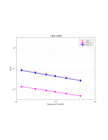
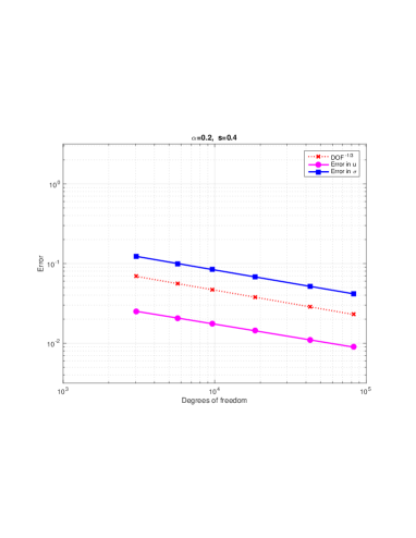
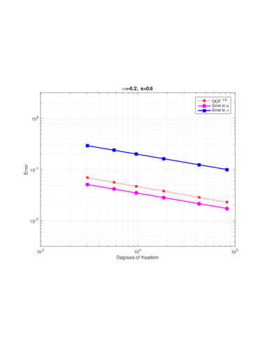
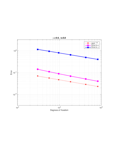
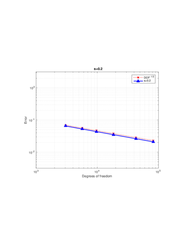
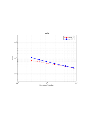
Now we give some numerical examples showing the asymptotic behavior
of the error proved in Theorem 5.3.
We solve Problem (5.2) with and
Recall that and .
In this case, assuming that (i. e. ), the solution is given by
where is a modified Bessel function of the second kind (see [24]).
We use prismatic elements given by a uniform mesh of triangles in and the
refinement given by (5.18) in the -direction. Observe that for
these meshes where denotes the degrees of freedom.
Moreover, we choose
as in Theorem 5.3 with , i. e., .
The next graphics show the order of the errors
and for several values of .
Figure 1. Rate of convergence: left , right .
Figure 2. Rate of convergence: left , right .
Finally, to solve (5.1), we need to approximate where
is the solution of (5.2).
We will use the approximations and obtained above.
Since is only an approximation in the -norm, one cannot expect that its
restriction to be a good approximation of . In order to obtain a better
approximation we will make a local correction of using also the computed .
This correction corresponds to a first order Taylor expansion,
indeed, the formula that we are going to prove in the next lemma is motivated by
We will prove that in this way we obtain an approximation in of at least the same order
than the mixed finite element approximation of (5.2).
Given and we introduce the jumps
If is not in the interior of an element in the partition of we choose
arbitrary an element containing it to evaluate (this is irrelevant because afterwards
we are going to integrate in ).
We will use the standard piecewise linear basis functions, namely, for ,
and
Lemma 5.4.
For any we have
(5.26)
Proof.
Since is piecewise constant one can see that
(5.27)
Let be the element containing . For , taking the function
supported in as test function in (2.7), we have
The next graphics show the order of the error
for Problem (5.1) with
which has as exact solution
Figure 3. Rate of convergence: left , right .
Remark 5.1.
The order of the error for the approximation
of in the -norm is probably not the optimal possible.
Indeed, with a more complicated postprocessing one could approximate
the solution of Problem (5.2) with order almost in
and, by the trace theorem
proved in [24, Proposition 2.5], one would have the same order
for the approximation of in the -norm. Therefore, it is reasonable
to expect a higher order in . Let us mention also that, as far as we know,
such a higher order error estimate has not been proved either for the standard method
analyzed in [24]. This problem requires a different analysis and
will be the object of our further research.
Acknowledgement: We thank Enrique Otárola for helpful comments.
References
[1]
Gabriel Acosta and Ricardo G. Durán.
The maximum angle condition for mixed and nonconforming elements:
application to the Stokes equations.
SIAM J. Numer. Anal., 37(1):18–36, 1999.
[2]
Gabriel Acosta and Ricardo G. Durán.
Divergence operator and related inequalities.
SpringerBriefs in Mathematics. Springer, New York, 2017.
[3]
Gabriel Acosta, Ricardo G. Durán, and María A. Muschietti.
Solutions of the divergence operator on John domains.
Adv. Math., 206(2):373–401, 2006.
[4]
Juan Pablo Agnelli, Eduardo M. Garau, and Pedro Morin.
A posteriori error estimates for elliptic problems with
Dirac measure terms in weighted spaces.
ESAIM Math. Model. Numer. Anal., 48(6):1557–1581, 2014.
[5]
Todd Arbogast and Abraham L. Taicher.
A linear degenerate elliptic equation arising from two-phase
mixtures.
SIAM J. Numer. Anal., 54(5):3105–3122, 2016.
[6]
Daniele Boffi, Franco Brezzi, Leszek F. Demkowicz, Ricardo G.
Durán,
Richard S. Falk, and Michel Fortin.
Mixed finite elements, compatibility conditions, and
applications, volume 1939 of Lecture Notes in Mathematics.
Springer-Verlag, Berlin; Fondazione C.I.M.E., Florence, 2008.
Lectures given at the C.I.M.E. Summer School held in Cetraro, June
26–July 1, 2006, Edited by Boffi and Lucia Gastaldi.
[7]
Daniele Boffi, Franco Brezzi, and Michel Fortin.
Mixed finite element methods and applications, volume 44 of
Springer Series in Computational Mathematics.
Springer, Heidelberg, 2013.
[8]
Seng-Kee Chua.
Weighted Sobolev inequalities on domains satisfying the chain
condition.
Proc. Amer. Math. Soc., 117(2):449–457, 1993.
[9]
R. R. Coifman and C. Fefferman.
Weighted norm inequalities for maximal functions and singular
integrals.
Studia Math., 51:241–250, 1974.
[10]
Lars Diening, Michael Ružička, and Katrin Schumacher.
A decomposition technique for John domains.
Ann. Acad. Sci. Fenn. Math., 35(1):87–114, 2010.
[11]
Irene Drelichman and Ricardo G. Durán.
Improved Poincaré inequalities with weights.
J. Math. Anal. Appl., 347(1):286–293, 2008.
[12]
Javier Duoandikoetxea.
Fourier analysis, volume 29 of Graduate Studies in
Mathematics.
American Mathematical Society, Providence, RI, 2001.
Translated and revised from the 1995 Spanish original by David
Cruz-Uribe.
[13]
R. G. Durán, A. L. Lombardi, and M. I. Prieto.
Supercloseness on graded meshes for finite element
approximation of a reaction-diffusion equation.
J. Comput. Appl. Math., 242:232–247, 2013.
[14]
Ricardo G. Durán and Fernando López García.
Solutions of the divergence and Korn inequalities on domains with
an external cusp.
Ann. Acad. Sci. Fenn. Math., 35(2):421–438, 2010.
[15]
Eugene B. Fabes, Carlos E. Kenig, and Raul P. Serapioni.
The local regularity of solutions of degenerate elliptic equations.
Comm. Partial Differential Equations, 7(1):77–116, 1982.
[16]
Richard S. Falk and John E. Osborn.
Remarks on mixed finite element methods for problems with rough
coefficients.
Math. Comp., 62(205):1–19, 1994.
[17]
José García-Cuerva and José L. Rubio de Francia.
Weighted norm inequalities and related topics, volume 116 of
North-Holland Mathematics Studies.
North-Holland Publishing Co., Amsterdam, 1985.
Notas de Matemática [Mathematical Notes], 104.
[18]
Ritva Hurri-Syrjänen.
An improved Poincaré inequality.
Proc. Amer. Math. Soc., 120(1):213–222, 1994.
[19]
Ritva Hurri-Syrjānen.
A weighted Poincaré inequality with a doubling weight.
Proc. Amer. Math. Soc., 126(2):545–552, 1998.
[20]
Douglas S. Kurtz.
Littlewood-Paley and multiplier theorems on weighted spaces.
Trans. Amer. Math. Soc., 259(1):235–254, 1980.
[21]
Alessandra Lunardi.
Interpolation theory, volume 16 of Appunti. Scuola Normale
Superiore di Pisa (Nuova Serie) [Lecture Notes. Scuola Normale Superiore di
Pisa (New Series)].
Edizioni della Normale, Pisa, 2018.
Third edition [of MR2523200].
[22]
Donatella Marini and Paola Pietra.
Mixed finite element approximation of a degenerate elliptic problem.
Numer. Math., 71(2):225–236, 1995.
[23]
Benjamin Muckenhoupt.
Weighted norm inequalities for the Hardy maximal function.
Trans. Amer. Math. Soc., 165:207–226, 1972.
[24]
Ricardo H. Nochetto, Enrique Otárola, and Abner J. Salgado.
A PDE approach to space-time fractional parabolic problems.
SIAM J. Numer. Anal., 54(2):848–873, 2016.
[25]
Ricardo H. Nochetto, Enrique Otárola, and Abner J. Salgado.
Piecewise polynomial interpolation in Muckenhoupt weighted
Sobolev spaces and applications.
Numer. Math., 132(1):85–130, 2016.
[26]
Katrin Schumacher.
Solutions to the equation in weighted Sobolev
spaces.
In Parabolic and Navier-Stokes equations. Part 2,
volume 81 of Banach Center Publ., pages 433–440. Polish Acad. Sci.
Inst. Math., Warsaw, 2008.