Matrix-oriented discretization methods for reaction-diffusion PDEs: comparisons and applications

Abstract

Systems of reaction-diffusion partial differential equations (RD-PDEs) are widely applied for modelling life science and physico-chemical phenomena. In particular, the coupling between diffusion and nonlinear kinetics can lead to the so-called Turing instability, giving rise to a variety of spatial patterns (like labyrinths, spots, stripes, etc.) attained as steady state solutions for large time intervals. To capture the morphological peculiarities of the pattern itself, a very fine space discretization may be required, limiting the use of standard (vector-based) ODE solvers in time because of excessive computational costs. We show that the structure of the diffusion matrix can be exploited so as to use matrix-based versions of time integrators, such as Implicit-Explicit (IMEX) and exponential schemes. This implementation entails the solution of a sequence of discrete matrix problems of significantly smaller dimensions than in the vector case, thus allowing for a much finer problem discretization. We illustrate our findings by numerically solving the Schnackenberg model, prototype of RD-PDE systems with Turing pattern solutions, and the DIB-morphochemical model describing metal growth during battery charging processes.

1 Introduction

We are interested in the numerical solution of reaction-diffusion partial differential equations (RD-PDEs) of the type

$$u_{t}=\ell(u)+f(u),\quad u=u(x,y,t),\quad with\quad(x,y)\in\Omega\subset\mathbb{R}^{2},\quad t\in]0,T],$$ (1)

with given initial condition $u(x,y,0)=u_{0}(x,y)$ and appropriate boundary conditions on the spatial domain. We assume that the diffusion operator $\ell$ is linear in $u$, while the function $f$ contains the nonlinear reaction terms. This setting can be generalized to the system case, which reads as

$$\begin{cases}u_{t}=\ell_{1}(u)+f_{1}(u,v),\\ v_{t}=\ell_{2}(v)+f_{2}(u,v),\quad with\quad(x,y)\in\Omega\subset\mathbb{R}^{2},\quad t\in]0,T].\end{cases}$$ (2)

RD-PDE systems describe mathematical models of interest in many classical scientific fields like chemistry [42, 8], biology [26, 22], ecology [23, 35], but also in recent applications concerning for example metal growth by electrodeposition [34, 18, 17], tumor growth [36], biomedicine [14] and cell motility [13]. In particular, since the pioneering work of Alan Turing at the origin of mathematical description of morphogenesis [41], it has been shown that the coupling between diffusion and nonlinear kinetics can lead to the so-called diffusion-driven or Turing instability, giving rise to a wide variety of spatial patterns (like labyrinths, spots, stripes, etc.) as stationary solutions to (2); see, e.g., [26, 3, 6, 18]. These models have been classically solved in a planar domain $\Omega$, however more recently certain physical applications have motivated the solution of (2) on stationary or time evolving surfaces where the diffusion $\ell(u)$ is defined in terms of the Laplace-Beltrami operator [11, 12, 21]. The numerical treatment of these models require a space discretization, and a time integration, commonly performed by Implicit-Explicit schemes [2, 31], or the Alternating Direction Integration (ADI) approaches [18, 34, 32]. It is well known that the Method of Lines (MOL) based on classical semi-discretizations in space (e.g. finite differences, finite elements) rewrites (1) as an ODE system

$$\dot{\bf u}=A{\bf u}+f({\bf u}),\quad{\bf u}(0)={\bf u}_{0}$$ (3)

where the entries of the matrix $A$ stem from the discretization of the spatial derivatives involved in the diffusion operator $\ell(u)$, while the vector ${\mathbf{u}}$ contains the coefficients for the approximation of the sought after function $u$, in the chosen basis. Analogous ODE equations are obtained by the semi-discretization of the PDE system (2), that is

$$\begin{cases}\dot{\bf u}=A_{1}{\bf u}+f_{1}({\bf u},{\bf v}),\quad{\bf u}(0)={\mathbf{u}}_{0},\\ \dot{\bf v}=A_{2}{\bf v}+f_{2}({\bf u},{\bf v}),\quad{\bf v}(0)={\bf v}_{0}.\end{cases}$$ (4)

We are interested in exploring time stepping strategies that can efficiently handle the nonlinear part, by judiciously exploiting the coefficient matrix structure in the linear part. In particular, we discuss the situation where the given domain is sufficiently regular so that the linear differential operator $\ell(u)$ can be discretized by means of a tensor basis; for instance, this is the case for finite difference methods, or for certain finite element techniques or spectral methods. In this framework, the physical space can be mapped into a so-called “logical space”, typically represented by a rectangle; see, e.g., [16]. To simplify the presentation, and to adhere to the application we are going to focus on, in the following we shall restrict the discussion to a rectangular domain, say $\Omega=[0,\ell_{x}]\times[0,\ell_{y}]$. With these premises, the discretization of the linear diffusion operator leads to a matrix $A$ of the form

$$A=I\otimes T_{1}+T_{2}^{T}\otimes I\in\mathbb{R}^{N_{x}N_{y}\times N_{x}N_{y}},$$ (5)

where $\otimes$ is the Kronecker operator, and $T_{1}$ ($T_{2}$) contains the approximation of the second order derivative in the $x$-direction ($y$-direction): $N_{x}$ and $N_{y}$ are the numbers of mesh interior nodes in the x- and y-directions, respectively. For example, in the case of finite differences $h_{x}=\ell_{x}/(N_{x}+1),\ h_{y}=\ell_{y}/(N_{y}+1)$ will be the corresponding space meshsizes.

With this hypotheses, at each time $t\in[0,T]$ it is possible to explicitly employ the matrix $U(t)\in\mathbb{R}^{N_{x}\times N_{y}}$ containing the same components of ${\mathbf{u}}(t)$, with $U_{i,j}(t)\approx u(x_{i},y_{j},t)$, that is, the rows and columns of $U$ explicitly reflect the space grid discretization of the given problem. The vector ${\mathbf{u}}$ corresponds to the vec operation of the matrix $U$, where each column of $U$ is stuck one after the other. In a finite difference discretization this implements a lexicographic order of the nodes in the rectangular grid. With this notation, for $A$ in (5) we have that $A{\mathbf{u}}={\rm vec}(T_{1}U+UT_{2})$. Then (3) can be written as the following differential matrix equation

$$\dot{U}=T_{1}U+UT_{2}+F(U),\quad U(0)=U_{0},$$ (6)

where $F$ is the nonlinear vector function $f({\mathbf{u}})$ evaluated componentwise, and ${\rm vec}(U_{0})={\mathbf{u}}_{0}$ is the initial condition. Analogously, under the same discretization framework, the system in (4) can be brought to the matrix form

$$\begin{cases}\dot{U}=T_{11}U+UT_{12}+F_{1}(U,V),\quad U(0)=U_{0},\\ \dot{V}=T_{21}V+VT_{22}+F_{2}(U,V),\quad V(0)=V_{0}\end{cases}$$ (7)

with obvious notation for the introduced quantities.

These matrix forms provide a quite different perspective at the time discretization level than classical approaches, allowing to significantly reduce the memory and computational requirements. The use of matrix-based approaches has only very recently been explored in a systematic manner, in the context of linear or quadratic matrix terms, such as the Sylvester and Riccati differential equations, see, e.g., [5, 4, 39]. In particular, matrix ODE equations like (6) - in the case when the term $F(U)$ allows for low-rank approximations - have been considered in [25]; in that article, the authors propose a low-rank strategy for matrix approximation in time based on Lie-Trotter and Strang splittings. Here, to complete the PDE approximation in the two cases above (6) and (7), we show that the standard time discretization strategies can be tailored to the matrix equation setting, with several numerical advantages.

The paper is structured as follows. After a brief survey in section 2 of methods usually applied to discretize in time (3) and its system counterpart, in section 3 we reformulate some of these methods in a matrix-oriented setting, that explicitly exploits the Kronecker form of the linear part of the problem. Among these, we consider the implicit-explicit Euler (IMEX Euler) and 2SBDF methods (IMEX-2SBDF), and low order exponential integrators (Exp Euler). Algorithmic details that make the matrix-oriented methods particularly efficient are discussed in section 3.3, where the reduced methods rEuler, rExp and rSBDF working in the spectral space are introduced. In section 4 we discuss the application of the matrix-oriented methods to the semilinear Heat equation, representative of (1) as test RD-PDE when the exact solution is known. We present a stability and convergence experimental study for the proposed numerical schemes together with comparisons of computational costs in order to emphasize the advantages of solving sequences of matrix problems with respect to the usual vector approach. In section 5, we extend the above reduced schemes to deal with RD-ODE matrix systems (7). In section 6, we present the features of diffusion-driven instability or Turing theory [3, 26] for pattern formation in nonlinear RD-PDE systems and the challenges for the numerical approximation of Turing pattern solutions; we solve the prototype Schnackenberg model [26] and the DIB-morphochemical model [18], representative of these pattern formations in different application contexts. All reported experiments are performed in Matlab [24] on a quadcore processor Intel Core(TM) i7-4770 CPI@3.40GHz, 16Gb RAM.

2 Classical vector methods

For the time stepping of (3) we can consider the following methods, where for the sake of simplicity we consider a constant timestep $h_{t}>0$ and the time grid $t_{n}=nh_{t}$, $n=0,1,\dots,N_{t}$ so that $({\bf u}_{n})_{ij}\approx u(x_{i},y_{j},t_{n})$ in each point $(x_{i},y_{j})$ of the discretized space:

1. IMEX methods.

   1. First order Euler: We discretized in time as ${\bf u}_{n+1}-{\bf u}_{n}=h_{t}(A{\bf u}_{n+1}+f({\bf u}_{n}))$, so that

      $$(I-h_{t}A){\bf u}_{n+1}={\bf u}_{n}+h_{t}f({\bf u}_{n}),\quad n=0,\dots,N_{t}-1,$$ (8)

      where ${\bf u}_{0}$ is given by the initial condition in (3); the linear part is treated implicitly, while the reaction (nonlinear) part $f$ is treated explicitly [2, 10, 31].

   2. Second order SBDF. The widely used IMEX 2-SBDF method [31, 2] applied to (3) yields

      $$3{\mathbf{u}}_{n+2}-4{\mathbf{u}}_{n+1}+{\mathbf{u}}_{n}=2h_{t}A{\mathbf{u}}_{n+2}+2h_{t}(2f({\mathbf{u}}_{n+1})-f({\mathbf{u}}_{n})),\quad n=0,1,\dots,N_{t}-2\\$$ (9)

      As usual, ${\mathbf{u}}_{0}$ is known, while a step of the first order IMEX-Euler scheme can be used to determine ${\mathbf{u}}_{1}$ ([31, 2]).

2. Exponential integrator. Exponential first order Euler method [15]:

   $${\bf u}_{n+1}=e^{h_{t}A}{\bf u}_{n}+h_{t}\varphi_{1}(h_{t}A)f({\bf u}_{n})$$ (10)

   where $e^{h_{t}A}$ is the matrix exponential, and $\varphi_{1}(z)=(e^{z}-1)/z$ is the first “phi” function [15].

3. ADI method. We consider the two-stage time stepping when ${\ell}(u)=\Delta u=u_{xx}+u_{yy}$ is the Laplace operator that approximates the reaction term in explicit way:

   $$\begin{split}&\frac{u_{ij}^{n+\frac{1}{2}}-u_{ij}^{n}}{h_{t}/2}=(u_{xx})_{ij}^{n+\frac{1}{2}}+(u_{yy})_{ij}^{n}+f(u_{ij}^{n}),\\ &\frac{u_{ij}^{n+1}-u_{ij}^{n+\frac{1}{2}}}{h_{t}/2}=(u_{xx})_{ij}^{n+\frac{1}{2}}+(u_{yy})_{ij}^{n+1}+f(u_{ij}^{n}).\end{split}$$ (11)

   Let $U_{n}\approx U(t_{n})\in\mathbb{R}^{N_{x}\times N_{y}}$. After discretization we obtain

   $$\begin{split}&\left(I-\frac{h_{t}}{2}T_{1}\right)U_{n+\frac{1}{2}}=\left(I+\frac{h_{t}}{2}T_{1}\right)U_{n}+\frac{h_{t}}{2}F(U_{n})\\ &{U_{n+1}\left(I-\frac{h_{t}}{2}T_{2}^{T}\right)=U_{n+\frac{1}{2}}\left(I+\frac{h_{t}}{2}T_{2}^{T}\right)+\frac{h_{t}}{2}F(U_{n})}.\end{split}$$ (12)

   We remark that the ADI method naturally treats the approximation in matrix terms, therefore it is the closest to our methodology.

3 Matrix formulation of classical methods

In this section we reformulate some of the time steppings of section 2 in matrix terms, by exploiting the Kronecker sum in (5). We then provide implementation details to make the new algorithms more efficient. To this end, we recall that $U(t)$ defines the matrix whose elements approximate at the time $t$ the values of $u(x_{i},y_{j},t)$ at the nodes $(x_{i},y_{j})$ in the discrete space, and $U_{n}\approx U(t_{n})$ such that ${\bf u}_{n}=vec(U_{n})$. We shall see that the matrix-oriented approach leads to the evaluation of matrix functions and to the solution of linear matrix equations with small matrices, instead of the solution of very large vector linear systems. We stress that the matrix formulation does not affect the convergence and stability properties of the underlying time discretization method. Rather, it exploits the structure of the linear part of the operator to make the computation more affordable. In particular, this allows one to refine the space discretization, so as to capture possible peculiarities of the problem; see, e.g., section 6.1.

In the following we derive the time iteration associated with the single differential equation (1) yielding the semi-discrete ODE matrix system (6) . A completely analogous iteration will be obtained for the ODE matrix system (7), see section 5.

3.1 Matrix-oriented first and second order IMEX methods

The matrix-oriented versions of the IMEX methods rely on the Kronecker form of $A$ in (5) and on its property that allows to trasform the vector linear system into a matrix linear equation to be solved, of much smaller size.

Consider the discretized times $t_{n}=nh_{t},\ n=0,\dots N_{t}$ with timestep $h_{t}>0$. Then adapting the one-step scheme in (8), to the differential matrix form (6), yields

$$U_{n+1}-U_{n}=h_{t}(T_{1}U_{n+1}+U_{n+1}T_{2})+h_{t}F(U_{n}),$$

which, after reordering, gives the following linear matrix equation, called the Sylvester equation,

$$(I-h_{t}T_{1})U_{n+1}+U_{n+1}(-h_{t}T_{2})=U_{n}+h_{t}F(U_{n}),\quad n=0,\dots,N_{t}-1.$$ (13)

Therefore, to obtain the next iterate $U_{n+1}$ the matrix approach for the IMEX Euler method requires the solution of a Sylvester equation at each time step, with coefficient matrices $(I-h_{t}T_{1})$, $(-h_{t}T_{2})$ and right-hand side $U_{n}+h_{t}F(U_{n})$. The numerical solution of (13) is described in section 3.3. The matrix equation (13) should be compared with the vector form, requiring the solution of a linear system of size $N_{x}N_{y}\times N_{x}N_{y}$ at each time step. It is important to realize that for a two-dimensional problem on a rectangular grid, the number of nodes required in each direction need not exceed a thousand, even in the case a fine grid is desired to capture possibly pathological behaviors. Hence, while the Sylvester equation above deals with, say, matrices of size $500\times 500$, the vector form deals with matrices and working vectors of size $250\,000\times 250\,000$. Arguably, these latter large matrices are very sparse and structured, so that strategies for sparse matrices can be exploited; nonetheless, the Sylvester equation framework allows one to employ explicit factorizations, also exploiting the fact that the coefficient matrices do not change with the time steps. Algorithmic details will be given in section 3.3.

As second order IMEX strategy for (6) we consider the two-step method IMEX-2SBDF seen in (9) for the vector formulation. For the matrix form, given the initial condition $U_{0}$, and a further approximation $U_{1}$ – obtained for instance by the IMEX Euler method – at each time step $t_{n+2}$ the method determines the following matrix equation

$$3U_{n+2}-4U_{n+1}+U_{n}=2h_{t}\left(T_{1}U_{n+2}+U_{n+2}T_{2}+2F(U_{n+1})-F(U_{n})\right),$$

which, after reordering, leads once again to the solution of a Sylvester equation in the unknown matrix $U_{n+2}$ given by

$$\left(3I-2h_{t}T_{1}\right)U_{n+2}+U_{n+2}\left(-2h_{t}T_{2}\right)=4U_{n+1}-U_{n}+2h_{t}(2F(U_{n+1})-F(U_{n})),\quad n=0,\dots,N_{t}-2.$$

The coefficient matrices are $3I-2h_{t}T_{1}$, $(-2h_{t}T_{2})$ and the right-hand side is $4U_{n+1}-U_{n}+2h_{t}(2F(U_{n+1})-F(U_{n}))$.

3.2 Exponential Euler method

A matrix-oriented version of the exponential Euler approach can exploit (5) in the computation of both the exponential and the phi-function. In particular, the following property of the exponential matrix is crucial

$$e^{h_{t}A}=e^{h_{t}(I\otimes T_{1}+T_{2}^{T}\otimes I)}=e^{h_{t}T_{2}^{T}}\otimes e^{h_{t}T_{1}}.$$

Therefore, for ${\bf u}={\rm vec}(U)$ we have

$$e^{h_{t}A}{\bf u}=\left(e^{h_{t}T_{2}^{T}}\otimes e^{h_{t}T_{1}}\right){\bf u}={\rm vec}(e^{h_{t}T_{1}}Ue^{h_{t}T_{2}}).$$

Moreover, the operation $v=h_{t}\varphi_{1}(h_{t}A)f=A^{-1}(e^{h_{t}A}f-f)$ can be performed by means of a two step procedure which, given $F$ such that $f={\rm vec}(F)$ delivers $V$ such that $v={\rm vec}(V)$:

1. Compute $\ G=e^{h_{t}T_{1}}Fe^{h_{t}T_{2}}$

2. Solve $\ T_{1}V+VT_{2}=G-F\quad\quad$ for $V$.

Therefore, the matrix-oriented version of the Exponential Euler method first computes the matrix exponential of multiples of $T_{1}$ and $T_{2}$ once for all. Then, it obtains the approximation $U_{n+1}$ by solving a Sylvester matrix equation at each time step. More precisely,

1. Compute $E_{1}=e^{h_{t}T_{1}}$, $E_{2}=e^{h_{t}T_{2}^{T}}$

2. For each $n$

   $${\rm Solve} \quad T_{1}V_{n}+V_{n}T_{2}=E_{1}F(U_{n})E_{2}^{T}-F(U_{n})$$ (14)

   $${\rm Compute} \quad U_{n+1}=E_{1}U_{n}E_{2}^{T}+V_{n}.$$

Several implementation suggestions are given in the next section. It is important to realize that to be able to solve (14) the two matrices $T_{1}$ and $-T_{2}$ must have disjoint spectra. Unfortunately, Neumann boundary conditions imply that both $T_{1}$ and $T_{2}$ are singular, leading to a zero common eigenvalue. To cope with this problem we employed the following differential matrix equation, mathematically equivalent to (6),

$$\dot{U}=(T_{1}-\sigma I)U+UT_{2}+(F(U)+\sigma U).$$ (15)

With this simple “relaxation” procedure the matrix $T_{1}-\sigma I$ is no longer singular, and has no common eigenvalues with $-T_{2}$, at the small price of including an extra linear term to the nonlinear part of the equation. We note that adding and subtracting the term $\sigma U$ to the ODE may be beneficial – though not strictly necessary – also for the other methods; thus in section 4.1 we include a stability analysis for all considered time integration strategies based on the relaxed matrix equation (15).

3.3 Implementation details

Whenever the matrix sizes are not too large, say up to a thousand, the previously described matrix methods can be made more efficient by computing a-priori a spectral decomposition of the coefficient matrices involving $T_{1}$ and $T_{2}$. In the following we shall assume that the two matrices are diagonalizable, so that their eigenvalue decompositions can be determined. Let them be $T_{k}=X_{k}\Lambda_{k}X_{k}^{-1}$, $k=1,2$, with $X_{k}$ nonsingular and $\Lambda_{k}={\rm diag}(\lambda_{1}^{(k)},\lambda_{2}^{(k)},\ldots)$ diagonal.

Let us first consider the IMEX Euler iteration in (13). Compute the $N_{x}\times N_{y}$ matrix $L_{i,j}=1/((1-h_{t}\lambda_{i}^{(1)})+(-h_{t}\lambda_{j}^{(2)}))$. Hence, at each iteration $n$ we can proceed as follows

• Compute $\widehat{U}_{n}=X_{1}^{-1}Q(U_{n})X_{2}\quad$ where $\quad Q(U_{n})=U_{n}+h_{t}F(U_{n})$;

• Compute $U_{n+1}=X_{1}(L\circ\widehat{U}_{n})X_{2}^{-1}$

where $\circ$ is the Hadamard (element by element) product. The second step performs the solution of the Sylvester equation by determining the solution entries one at the time, in the eigenvector bases, and then the result is projected back onto the original space to get $U_{n+1}$ [38]. Proceeding in the same manner, the corresponding version for IMEX-2SBDF can be derived. Letting this time $L_{i,j}=1/((3-2h_{t}\lambda_{i}^{(1)})+(-2h_{t}\lambda_{j}^{(2)}))$ at each time iteration $n$ we have:

• Compute $\widehat{U}_{n}=X_{1}^{-1}Q(U_{n},U_{n+1})X_{2}\quad$ where $\quad Q(U_{n},U_{n+1})=4U_{n+1}-U_{n}+2h_{t}(2F(U_{n+1})-F(U_{n}))$;

• Compute $U_{n+1}=X_{1}(L\circ\widehat{U}_{n})X_{2}^{-1}$.

In the following numerical experiments we will call these methods: reduced IMEX-Euler (rEuler) and reduced 2SBDF (rSBDF). Whenever the RD-PDE problem is linear, that is $f(u)=\alpha u+\beta$, the computation further simplifies, since all time steps can be performed in the eigenvector basis, and only at the final time of integration the approximate solution is interpolated back to the physical basis; see section 4.

In a similar way, the matrix-oriented exponential Euler integrator described in section 3.2 can be rewritten as

1. Compute $\widehat{e}_{k}={\rm diag}(e^{h_{t}\lambda_{1}^{(k)}},e^{ht\lambda_{2}^{k)}},\ldots)$, $k=1,2;$ $\widehat{E}=\widehat{e}_{1}\widehat{e}_{2}^{*}$ and $\widehat{L}_{i,j}=(h_{t}\lambda_{i}^{(1)}+h_{t}\lambda_{j}^{(2)})^{-1}$, with $\widehat{E},\widehat{L}\in{\mathbb{C}}^{N_{x}\times N_{y}}$.

2. For each $n$,

3. Compute $\widehat{F}_{n}=X_{1}^{-1}F(U_{n})X_{2}$          % Project $F(U_{n})$ on the eigenbases;

4. Compute $G=\widehat{E}\circ\widehat{F}_{n}-\widehat{F}_{n}$             % Apply exp and form the Sylvester eqn rhs;

5. Compute $V=\widehat{L}\circ G$                     % Solve the Sylvester eqn;

6. Compute $U_{n+1}=X_{1}(\widehat{E}\circ(X_{1}^{-1}U_{n}X_{2})+V)X_{2}^{-1}$      % Compute the next iterate

In the following numerical experiments we will call this method reduced Exp (rExp).

If the “relaxation” approach corresponding to (15) is considered, the quantity $F_{\sigma}(U)=F(U)+\sigma U$ replaces $F(U)$ in the algorithm above, while the spectral decomposition of $T_{1}(\sigma)=T_{1}-\sigma I$ replaces that of $T_{1}$.

4 The semilinear heat equation

We start by specializing the matrix methods of the previous sections to the case of the following Heat Equation (HE) with linear source (reaction) term and zero Neumann boundary conditions (BCs):

$$\begin{cases}u_{t}=d\Delta u+\alpha u\quad(x,y)\in\Omega\subset\mathbb{R}^{2},\ t\in]0,T],\ \\ (\boldsymbol{n}\nabla u)_{|\partial\Omega}=0,\quad u(x,y,0)=u_{0}(x,y),\end{cases}$$ (16)

with $d\in\mathbb{R_{+}}$ the diffusion coefficient, $\alpha\in\mathbb{R}$ the reaction coefficient and $\Omega=[0,\ell_{x}]\times[0,\ell_{y}]$ a rectangular domain. We consider the initial condition $u_{0}(x,y)=A_{0}\cos(c_{x}x)\cos(c_{y}y)$, for which the exact solution of (16) is given by $u^{*}(x,y,t)=e^{(\alpha-(c_{x}^{2}+c_{y}^{2})d)t}u_{0}(x,y)$.

For the numerical treatment, we consider a finite difference approximation for spatial derivatives based on the Extended Central Difference Formulas (ECDF) [1, 34]. These schemes consider the approximation of the Neumann BCs with the same order of schemes used in the interior domain, so that no reduction of order arises near the boundaries. In particular, we apply the scheme of order $p=2$ as follows. Let us discretize the domain $\Omega$ with $N_{x}$ and $N_{y}$ interior points, giving step sizes $h_{x}=\ell_{x}/(N_{x}+1)$ and $h_{y}=\ell_{y}/(N_{y}+1)$. Let $U_{ij}(t)\approx u(x_{i},y_{j},t)$, for $i=1,\dots,N_{x}$, $j=1,\dots,N_{y}$ be the values of the approximate solution at the interior mesh nodes, and let ${\mathbf{u}}={\rm vec}(U)$.

Let $T_{x}\in\mathbb{R}^{N_{x}\times N_{x}}$ and $T_{y}\in\mathbb{R}^{N_{y}\times N_{y}}$ be the usual tridiagonal matrices corresponding to the approximation of the second order derivatives in (16) by central differences (order $p=2$), along the $x$ and $y$ directions, and zero Neumann BCs approximation. More precisely, $T_{x}=diag(1,-2,1)+B$, and similarly for $T_{y}$, with corresponding dimensions, where the BCs term (see [34, 32]) is given by

$$B=\frac{2}{3}\begin{bmatrix}2&-\frac{1}{2}&\cdots&0&0\\ 0&0&\cdots&\cdots&0\\ \vdots&&&&\vdots\\ 0&\cdots&&-\frac{1}{2}&2\end{bmatrix}.$$ (17)

Therefore, the semi-discretization of (16) in vector form is given by

$$\dot{\bf u}=A{\bf u}+\alpha{\bf u}\quad{\bf u}(0)={\bf u}_{0},$$ (18)

where

$$A=d\widetilde{\Delta},\qquad\widetilde{\Delta}=\frac{1}{h_{x}^{2}}(I_{y}\otimes T_{x})+\frac{1}{h_{y}^{2}}(T_{y}\otimes I_{x})\in\mathbb{R}^{N_{x}N_{y}\times N_{x}N_{y}}$$ (19)

while its matrix counterpart becomes

$$\dot{U}=T_{1}U+UT_{2}+\alpha U,\quad\quad U(0)=U_{0},\quad T_{1}=\frac{d}{h_{x}^{2}}T_{x},\quad T_{2}=\frac{d}{h_{y}^{2}}T_{y}^{T}.$$ (20)

The solution of the Heat equation can take full advantage of the matrix formulation because of the linearity of the reaction term, see section 3.3. In Algorithm 1 we report the reduced IMEX-Euler method all in the eigenvector space. Note that the computational cost is thus kept to the minimum.

Algorithm 1 Reduced-Sylvester method for the Heat Equation

  Compute $X_{k},\Lambda_{k}$, $k=1,2$ such that $T_{1}=X_{1}\Lambda_{1}X_{1}^{-1}$, $T_{2}=X_{2}\Lambda_{2}X_{2}^{-1}$

  $\hat{U}_{1}=X_{1}^{-1}U_{0}X_{2}$

  $L_{i,j}=1./(\Lambda_{1}(i,i)+\bar{\Lambda}_{2}(j,j))$

  for $n=1:N_{t}$ do

     $\hat{U}_{1}=L\circ(\hat{U}_{1}+\alpha h_{t}\hat{U}_{1})$

  end for

  $U_{1}=X_{1}\hat{U}_{1}X_{2}^{-1}$

If time discretization is performed by the reduced Euler exponential integrator rExp we can take full advantage of the linearity of the operator, by including the constant term $\alpha$ into the $x$-direction matrix, thus avoiding the use of the term involving the function $\varphi_{1}$. The resulting expression for the next iterate is thus given by

$${\mathbf{u}}_{n+1}=e^{h_{t}(A+\alpha I)}{\mathbf{u}}_{n},$$ (21)

and $h_{t}(A+\alpha I)=I\otimes(T_{1}+h_{t}\alpha I)+T_{2}^{T}\otimes I$. By first computing the eigenvalue decompositions of $T_{1}+h_{t}\alpha I$ and of $T_{2}$ (which give the corresponding matrices $E$, $X_{1}$ and $X_{2}$), we obtain the matrix iteration in the eigenvector basis,

$$\widehat{U}_{0}=X_{1}^{-1}U_{0}X_{2},\qquad\widehat{U}_{n+1}=\widehat{E}\circ\widehat{U}_{n},\,\,n=0,1,\ldots$$

where the elements of $\widehat{E}$ are all possible products of eigenvalues of $T_{1}+h_{t}aI$ and $T_{2}$ (see the general description in section 3.3). Only at the final integration time the solution is projected back onto the physical basis as $U_{*}=X_{1}\widehat{U}_{*}X_{2}^{-1}$.

4.1 Stability analysis

In this subsection, we present a stability analysis of the schemes proposed in the previous sections, by considering as PDE test problem the Heat Equation in (16) and its vector form semi-discretization (18). By using the spectral decomposition $A=Q\Lambda Q^{-1}$, we can define $\widetilde{\bf u}=Q^{-1}{\bf u}$, and work with the associated scalar test problem for each component $\widetilde{u}=(\widetilde{\bf u})_{j},\lambda=\lambda_{j}$ where $\lambda_{j}=(\Lambda)_{jj}$. Note that it holds that $\lambda=d\widetilde{\lambda}$ where $\widetilde{\lambda}_{j}$ is an eigenvalue of $\widetilde{\Delta}$ in (19). In general, we can thus consider the scalar ODE test problem

$$\dot{\widetilde{u}}=\lambda\widetilde{u}+\alpha\,\widetilde{u}$$ (22)

where $\lambda\in\mathbb{R}_{-}$ models the diffusion and $\alpha\in\mathbb{R}$ models the reaction. The exact solution of (22) is $u^{*}(t)=u_{0}e^{(\lambda+\alpha)t}$ that goes to zero for $t\rightarrow\infty$ (i.e. it is asymptotically stable) if and only if

$$\lambda+\alpha<0\quad\Longleftrightarrow\quad\alpha<-\lambda.$$ (23)

If $h_{t}$ is the time stepsize, let be $\xi=\lambda h_{t}$ and $\mu=\alpha h_{t}$, then the region in the plane $(\xi,\mu)$, with $\xi<0$ where stationary solutions can be obtained is given by the half-plane $\mu<-\xi$. (In the following with some abuse of notation we use $u$ instead of $\widetilde{u}$ in (22).) Following (15), we relax the equation with $\sigma u=-\omega\alpha u$ in (22) as follows:

$$\dot{u}=(\lambda u-\sigma u)+(\alpha u+\sigma u)\ \Longleftrightarrow\ \dot{u}=\lambda_{\omega}u+\alpha_{\omega}\,u,\quad\quad 0\leq\omega\leq 1$$ (24)

where $\lambda_{\omega}=(\lambda+\omega\alpha)$ and $\alpha_{\omega}=(1-\omega)\alpha$. For $\omega\in[0,1]$ the problem (24) is equivalent to (22), that is it admits the same solution $u^{*}$, and for $\omega=0$ we find exactly (22). Moreover, by (23) we need to enforce the constraints

$$\lambda_{\omega}<0,\qquad\lambda_{\omega}+\alpha_{\omega}=\lambda+\alpha<0.$$ (25)

Our aim is twofold: (i) identify the stability regions $R_{met}$ in the $(\xi,\mu)$ plane of the considered methods, where these schemes are able to reproduce the asymptotic stationary behavior of the theoretical solution; (ii) identify the restrictions on the timestep $h_{t}$ in terms of the diffusion and reaction terms.

We recall that the relaxed approach needs to be used to apply the rExp integrator to the general nonlinear model, since $A$ in (18) is singular. Although in this linear case the general Euler exponential method would not be required, we believe that the analysis still provides valuable indications of the stability properties of the methods towards the general nonlinear setting.

The IMEX Euler method for (24) is given by $u_{n+1}=u_{n}+h_{t}(\lambda_{\omega}u_{n+1}+\alpha_{\omega}u_{n})$, from which we get

$$(1-\lambda_{\omega}h_{t})u_{n+1}=(1+\alpha_{\omega}h_{t})u_{n}.$$ (26)

Letting $\xi=\lambda_{\omega}h_{t}<0$ and $\mu=\alpha_{\omega}h_{t}$, we have $\displaystyle u_{n+1}=\frac{(1+\mu)}{(1-\xi)}u_{n}.$ Then, taking into account the constraints in (25), the EIMEX numerical solution is asymptotically stable in (see Figure 1 (left) dashed lines)

$${\cal R}_{EIMEX}=\left\{(\xi,\mu)\in\mathbb{R}_{-}\times\mathbb{R}\ |\quad\displaystyle\frac{|1+\mu|}{|1-\xi|}<1\right\}\quad\Leftrightarrow\quad\xi-2<\mu<-\xi.$$

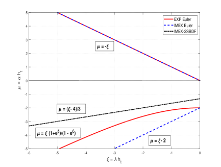
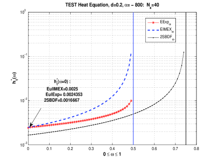
Figure 1: Heat equation - Left plot: stability regions in the plane $(\xi,\mu)$ for IMEX and EXP Euler methods and the 2-SBDF method applied to the linear test problem (18). Right plot: For $d=0.2$, $\alpha=-800$ in (16) and $N_{x}=N_{y}=40$ meshpoints in the spatial domain $\Omega=[0,1]\times[0,1]$, we show the critical timesteps of all methods in dependence of the relaxation parameter $\omega\in[0,1]$.

Explicitly writing $\mu$ and $\xi$, the bound $\mu>\xi-2$ allows us to determine possible timestep restrictions. Indeed, the bound $\mu>\xi-2$ corresponds to

$${\cal F}_{EIMEX}(h_{t},\lambda,\alpha,\omega):=[(1-2\omega)\alpha-\lambda]h_{t}+2>0.$$ (27)

A detailed analysis shows that this condition is always satisfied for all considered parameters, except if $(1-2\omega)\alpha<\lambda<0$, in which case the timestep constraint $h_{t}<2/(\lambda-(1-2\omega)\alpha)$. Since this condition must hold for all $\lambda$s, we can determine the critical stepsize in correspondence of the worst case as

$$h_{t}<\frac{2}{\lambda_{M}-(1-2\omega)\alpha}=:h_{crit}(\omega),$$ (28)

where $\lambda_{M}=\max_{j=1,\dots,N_{x}\cdot N_{y}}\lambda_{j}(A)=d\max_{j}\widetilde{\lambda}_{j}(\widetilde{\Delta})<0$. The curve of the critical stepsize $h_{crit}(\omega)$, as a function of $\omega\in[0,1]$, is shown in Figure 1 (right) for the case $d=0.2$, $\alpha=-800$, and $\lambda_{M}$ computed numerically for $N_{x}=N_{y}=40$ meshpoints in the spatial domain $\Omega=[0,1]\times[0,1]$. It is easy to see that the timestep restriction arises only for $\omega<1/2$.

A similar analysis for the Exponential Euler method determines the following stability region (see Figure 1 (left) red continuous line):

$${\cal R}_{EEXP}=\left\{(\xi,\mu)\in\mathbb{R}_{-}\times\mathbb{R}\ |\quad\displaystyle|\mu\frac{e^{\xi}-1}{\xi}+e^{\xi}\displaystyle|<1\right\}\quad\Leftrightarrow\quad\xi\frac{1+e^{\xi}}{1-e^{\xi}}<\mu<-\xi.$$

By substituting $\xi=\lambda_{\omega}h_{t}$ and $\mu=\alpha_{\omega}h_{t}$ the lower bound for $\mu$ implies the timestep restriction $-(\lambda_{\omega}+\alpha_{\omega})e^{\lambda_{\omega}h_{t}}-(\lambda_{\omega}-\alpha_{\omega})>0$, which is equivalent to requiring

$${\cal F}_{EEXP}(h_{t},\lambda,\alpha,\omega):=-(\lambda+\alpha)e^{(\lambda+\omega\alpha)h_{t}}+[(1-2\omega)\alpha-\lambda]>0.$$ (29)

Once again, a detailed analysis of the sign shows that only for $(1-2\omega)\alpha<\lambda<0$ we determine a constraint by identifying the critical timestep $h_{t}(\omega)$ as $\omega$ varies. This is obtained by looking for the zeros $z^{*}$ of ${\cal F}_{EEXP}(z,\lambda_{M},\alpha,\omega)$ for $\omega\in[0,1]$. For the same PDE data as for the IMEX Euler method, the curve of these zeros $z^{*}=h_{t}^{*}(\omega),\omega\in[0,1]$ is reported in Figure 1 (right). Again, the timestep restriction arises only for $\omega<1/2$.

As shown in [34], the stability region for the second order IMEX 2-SBDF method (9) in the half-plane $(\xi,\mu)$, $\xi<0$ can be studied by the roots $|z_{1,2}(\xi,\mu)|$ of the second order characteristic polynomial associated to (9) when applied to the linear test problem:$(3-2\xi)z^{2}-4(\mu+1)z+1+2\mu=0.$ Hence, we have the stability region given by (see Figure 1 (left) dash-dot line)

$${\cal R}_{SBDF}=\left\{(\xi,\mu)\in\mathbb{R}_{-}\times\mathbb{R}\ |\quad|z_{1,2}(\xi,\mu)|\leq 1\right\}\quad\Leftrightarrow\quad\frac{\xi-4}{3}<\mu<-\xi.$$

Simple algebra shows that the same result is obtained if we consider the relaxed test problem (24) and $\xi=\lambda_{\omega}h_{t}$ and $\mu=\alpha_{\omega}h_{t}$. Again, the lower bound for $\mu$ implies the restriction $(3\alpha_{\omega}-\lambda_{\omega})h_{t}<-4$ on the timestep $h_{t}$, which is equivalent to requiring

$${\cal F}_{SBDF}(h_{t},\lambda,\alpha,\omega)=[(3-4\omega)\alpha-\lambda]h_{t}+4>0$$ (30)

Similar arguments as above imply that the constraint on $h_{t}$ is given if $\ (3-4\omega)\alpha<\lambda<0$, in which case $h_{t}<\displaystyle\frac{4}{\lambda-(3-4\omega)\alpha}$. Having to hold for all $\lambda$s, the critical timestep can be found by the worst case as:

$$h_{t}<\displaystyle\frac{4}{\lambda_{M}-(3-4\omega)\alpha}=:h_{crit}(\omega).$$ (31)

In Figure 1 (right) we report the critical timesteps (31) $h_{t}^{*}(\omega)$, for $\omega\in[0,1]$, for again the same PDE data. In this case $\alpha<0$ and stepsize restrictions arise only for $0\leq\omega<3/4$.

For the case $\omega=0$, that is without relaxation, the critical timesteps for the considered schemes are: $h_{t}^{EIMEX}=0.0025,h_{t}^{EEXP}=0.0024353,h_{t}^{2SBDF}=0.0016667$. (Note that these values can change for different space discretization values of $N_{x},N_{y}$.) By increasing the relaxation parameter $\omega$ until $\omega^{*}$ less stringent bounds arise, that is for all schemes an improvement in the stability requirements are obtained. The best gain is obtained by EIMEX, followed by EEXP and then by the more demanding second order scheme. This behavior is to be expected, due to the size of the respective stability regions shown in Figure 1 (left). For $\omega\geq\omega^{*}$ the methods are unconditionally stable, with $\omega^{*}=0.5$ for EEIMEX and EEXP, with $\omega^{*}=0.75$ for 2SBDF. It is worth noting that the application of the reduced Exponential Euler method for the Heat Equation in (21) corresponds to the relaxation $\omega=1$ and then, for $\alpha<0$, the method will not require any timestep restriction, then it is unconditionally stable.

Remark 4.1.1.

For the scalar linear ODE (22) the relaxed $\omega-$schemes correspond to applying in time an implicit approximation for the diffusion part in $\lambda$, and a classical $\theta-$ method for the reaction part. Hence, the relaxed IMEX Euler (26) for $\omega=0$ is equivalent to $EIMEX$, whereas for $\omega=1$ it corresponds to the fully implicit Euler method. The determined stability properties are thus expected. For the other relaxed schemes, we are not aware of similar stability results. It is worth mentioning that whenever the nonlinear term $f(u)$ includes a linear term with negative coefficient, the $\sigma$-correction in (15) simply corresponds to moving this linear term to the diffusion part of the expression.

4.2 Numerical results

In this section we experimentally explore the performance of the considered methods, that is rEuler, rsbdf, ADI and rExp, on the simple model matrix problem

$$\dot{U}=T_{1}U+UT_{2}+\alpha U,\quad U(0)=U_{0}.$$ (32)

where $T_{1},T_{2}$ are given in (20). According to (15), for rExp we actually solve the differential matrix equation $\dot{U}=(T_{1}+\alpha I)U+UT_{2}$.

Throughout this set of experiments we solve (16) on $\Omega=[0,1]\times[0,1]$, with the parameter choice $\alpha=-800$, $d=0.2$, $c_{x}=2$, $c_{y}=1$, $A_{0}=1$, $T_{f}=0.1$ and $N_{x}=N_{y}$ in the spatial meshgrid.

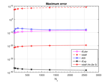
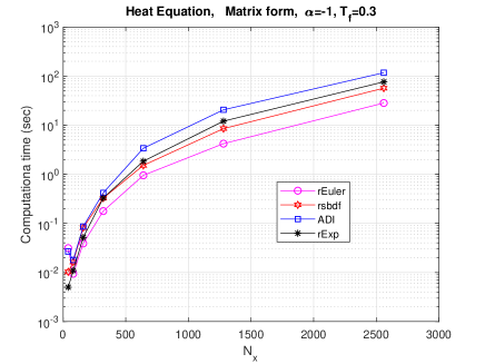
Figure 2: Heat equation with $d=0.2$, $\alpha=-800$. Left plot: Error of various reduced time integrators in matrix form for $h_{t}=10^{-3}$ (and also for $h_{t}=2\,10^{-3}$ in rSBDF). Right plot: Computational costs for all methods for $h_{t}=10^{-3}$.

To experimentally test the stability analysis of the previous section in the matrix case as the problem dimension increases, we consider two critical time steps, and vary $N_{x}$ as $N_{x}^{k}=40\cdot 2^{k}$ for $k=0,...,6$. The left plot of Figure 2 reports the behavior of the maximum (spatial) error for the solution at the final time $T_{f}$ for all methods for $h_{t}=10^{-3}$ (for rSBDF the history for $h_{t}=2\,10^{-3}$ is also reported). The plot confirms the analysis of the previous section: for the value $h_{t}=2\,10^{-3}$ falling outside the region of stability of the method, rSBDF provides an unacceptably high error, whereas the error behaves as expected by the convergence theory for the smaller value $h_{t}=1\,10^{-3}<h_{t}^{cr}$. The plot also confirms that for the linear problem the exponential method is exact in exact arithmetic, thus the displayed error is only due to the use of finite precision arithmetic in the computation of the spectral information.

Figure 2(right) reports on the computational cost (time in seconds) of all methods as the problem size grows. For the considered matrix dimensions, all methods behave somewhat similarly, although the use of the reduced strategy appears to be very beneficial. Note that for the largest values of $N_{x}$, the Kronecker form of the problem would have a diffusion matrix of size $6\cdot 10^{6}$, which would be extremely hard to handle for a large number of times steps, while limiting the type of time stepping methods to be employed. These considerations are particularly important in the case of systems of nonlinear equations, as considered in the next section. To illustrate this point, in Table 1 we report the CPU times of a full run with the standard vector-oriented IMEX scheme, compared with the reduced Euler approach. For this experiment, we consider $\alpha=-1$ and $T_{f}=0.3$, so that there is no restriction on the time step $h_{t}$. Moreover, we fix the ratio $\nu=\frac{h_{t}}{h_{x}^{2}}$ to preserve the order of convergence. Starting from $h_{t}^{1}=10^{-2}$, $N_{x}=32$ and $h_{x}=\frac{1}{N_{x}+1}$, $h_{t}$ is halved at each step $k$, that is $h_{t}^{k}:=\frac{h_{t}}{2^{k}}$ for $k=0,1,2...$, and $h_{x}^{k}:=\frac{h_{x}^{k-1}}{\sqrt{2}}$. In the vector case, an LU factorization with pivoting of the coefficient matrix is performed a-priori, so that only sparse triangular solves are performed at each iteration with the $N_{x}^{2}\times N_{x}^{2}$ factors. For larger values of $N_{x}$, a preconditioned iterative solver would be required to solve such very large linear system.

$N_{x}$	$32$	$45$	64	90	128	180	256	362
Vector	0.0414	0.0115	0.0398	0.1366	0.7899	3.1548	13.750	66.562
rEuler	2.3e-3	2.7e-3	6.3e-3	0.0143	0.0336	0.0878	0.1824	0.5699

Table 1: Heat equation for $\alpha=-1$ and $d=0.2,T_{f}=0.3$: Computational times in seconds for the IMEX Euler method solved in vector form by direct solver and in matrix form by the reduced method rEuler.

5 Reaction-diffusion PDE systems: matrix approach

In this section we apply the matrix-oriented approach to an RD-PDE model with nonlinear reaction terms and zero Neumann boundary conditions, given in general by:

$$\begin{cases}u_{t}=d_{1}\Delta u+f_{1}(u,v),\quad(x,y)\in\Omega\subset\mathbb{R}^{2},\ t\in]0,T]\\ v_{t}=d_{2}\Delta v+f_{2}(u,v),\\ (n\nabla u)_{|\partial\Omega}=(n\nabla v)_{|\partial\Omega}=0\\ u(x,y,0)=u_{0}(x,y),v(x,y,0)=v_{0}(x,y)\end{cases}$$ (33)

The Method of Lines for (33), based on the finite difference space discretization in (20), yields the following system of ODE matrix equations:

$$\begin{cases}U^{\prime}=d_{1}(T_{1}U+UT_{2})+F_{1}(U,V)\\ V^{\prime}=d_{2}(T_{1}\,V+V\,T_{2})+F_{2}(U,V)\\ U(0)=U_{0},V(0)=V_{0}.\end{cases}$$ (34)

As in section 3, the matrix form of the classical ODE methods can be derived for (34), giving rise to the solution of the following Sylvester matrix equations at each timestep $t_{n}$,

$$\begin{cases}S_{1}U_{n+1}+U_{n+1}S_{2}=Q_{1}^{n},\\ R_{1}V_{n+1}+V_{n+1}R_{2}=Q_{2}^{n},\quad n=0,\dots,N_{t}-1\quad\quad U_{0},V_{0}\ \mbox{given}\end{cases}$$ (35)

where $Q_{k}^{n}=Q_{k}^{n}(U_{n},V_{n}),k=1,2$ in the case of a one step method (like IMEX Euler method in the previous sections) and $Q_{k}^{n}=Q_{k}^{n}(U_{n-1},V_{n-1},U_{n},V_{n})$ (with $U_{0},U_{1}$ given) for a two-step scheme. Recalling the procedure of section 3.1, for IMEX-Euler we have

$$S_{1} = I-h_{t}d_{1}T_{1},\,\,S_{2}=-h_{t}d_{1}T_{2},\quad R_{1}=I-h_{t}d_{2}T_{1},\,\,R_{2}=-h_{t}d_{2}T_{2},$$ (36)

$$Q_{1}^{n} = U_{n}+h_{t}F_{1}(U_{n},V_{n}),\quad\,Q_{2}^{n}=V_{n}+h_{t}F_{2}(U_{n},V_{n}),$$

while for IMEX-2SBDF we have

$$S_{1} = 3I-2h_{t}d_{1}T_{1},\,\,S_{2}=-2h_{t}d_{1}T_{2},\,\quad R_{1}=3I-2h_{t}d_{2}T_{1},\,R_{2}=-2h_{t}d_{2}T_{2},$$

$$Q_{1}^{n} = 4U_{n}-U_{n-1}+2h_{t}(F_{1}(U_{n},V_{n})-F_{1}(U_{n-1},V_{n-1})),$$ (37)

$$Q_{2}^{n} = 4V_{n}-V_{n-1}+2h_{t}(F_{2}(U_{n},V_{n})-F_{2}(U_{n-1},V_{n-1})).$$

Analogously to section 3.2, also the matrix-oriented version of the exponential method can be derived for the RD systems. In particular, letting once again $E_{1,1}=e^{h_{t}d_{1}T_{1}}$, $E_{1,2}=e^{h_{t}d_{1}T_{2}^{T}}$, and $E_{2,1}=e^{h_{t}d_{2}T_{1}}$, $E_{2,2}=e^{h_{t}d_{2}T_{2}^{T}}$ we obtain

$$U_{n+1} = E_{11}U_{n}E_{12}^{T}+Y_{n},\,\,\quad{\rm where}\quad\,(d_{1}T_{1}-\sigma I)Y_{n}+Y_{n}(d_{1}T_{2})=E_{11}\widetilde{F}_{1}(U_{n},V_{n})E_{12}^{T}$$ (38)

$$V_{n+1} = E_{21}V_{n}E_{22}^{T}+Z_{n},\,\,\quad{\rm where}\quad\,(d_{2}T_{1}-\sigma I)Z_{n}+Z_{n}(d_{2}T_{2})=E_{21}\widetilde{F}_{2}(U_{n},V_{n})E_{22}^{T},$$ (39)

where $\sigma$ is as described in section 3.2, while $\widetilde{F}_{1}(U_{n},V_{n})=F_{1}(U_{n},V_{n})+\sigma U_{n}$ and $\widetilde{F}_{2}(U_{n},V_{n})=F_{2}(U_{n},V_{n})+\sigma V_{n}$. In particular, the approach requires the solution of two Sylvester equations per step, which is the same cost as for the IMEX procedure, together with matrix-matrix multiplications with the exponentials. As already discussed for the single equation case, these costs can be significantly reduced by working in the eigenvector basis of $T_{1}$ and $T_{2}$. A Matlab implementation of the rEuler and rExp methods is reported in the Appendix.

6 Nonlinear reaction-diffusion systems with Turing solutions

Reaction-diffusion systems like (33) arise in several scientific applications and describe mathematical models where the unknown variables can have different physical meaning, for example chemical concentrations, cell densities, predator-prey population sizes, etc. Ranging from ecology to bio-medicine, depending on the parameters in the model kinetics $f_{1},f_{2}$, different kinds of solutions can be studied, for example traveling waves or oscillating dynamics. We are interested in diffusion-driven or Turing instability solutions of (33), arising from the perturbation of a stable spatially homogeneous solution. More precisely, let $(u_{e},v_{e})$ be the stable solution to the homogeneous equations (33) with no diffusion, that is $f_{1}(u_{e},v_{e})=0=f_{2}(u_{e},v_{e})$. Adding diffusion can force spatial instability to take place, leading to an asymptotic interesting spatial pattern (so-called Turing pattern), characterized by structures like spots, worms, labyrinths, etc. More recently, in [27, 28] the authors proved that the transient dynamics is important for pattern formation. In particular, the concept of reactivity describing the short-term transient behavior, is necessary for Turing instabilities. Let ${\bf w}=(u,v)$ and let $J=J(u_{e},v_{e})=\begin{bmatrix}f_{1,u}&f_{1,v}\\ f_{2,u}&f_{2,v}\end{bmatrix}|_{{\bf w}_{e}}$ be the Jacobian of the linearized ODE system associated to (33) evaluated at the spatially homogeneous solution ${\bf w}_{e}=(u_{e},v_{e})$. The spatially homogeneous solution ${\bf w}_{e}=(u_{e},v_{e})$ is stable if the eigenvalues of $J$ all have negative real part, that is $J$ is a stable matrix. In [27] the authors defined ${\bf w}_{e}$ as reactive equilibrium if the largest eigenvalue of the symmetric part of $J$ is positive:

$$\lambda_{\max}(H(J))>0,\quad\quad H(J)=(J+J^{T})/2.$$

We recall that $J$ may be stable, while $H(J)$ is not stable, that is $H(J)$ has at least one strictly positive eigenvalue. This key feature is typical of stable highly non-normal matrices [40]. If the initial condition ${\bf w}_{0}(x,y)=(u_{0}(x,y),v_{0}(x,y))$ in (33) is a small (random) perturbation to ${\bf w}_{e}$, the RD-PDE solution in the initial transient, say ${\bf v}(x,y,t)$, is governed by the linearization

$${\bf v}_{t}=D\,\Delta{\bf v}+J{\bf v},\quad D=diag(d_{1},d_{2}).$$

By applying the Fourier transform $\widetilde{\bf v}({\bf k},t)=\int_{-\infty}^{\infty}e^{i(k_{x}x+k_{y}y)t}{\bf v}(x,y,t)dxdy$  this equation becomes the linear ODE system

$$\widetilde{\bf v}^{\prime}=\widetilde{J}\widetilde{\bf v},\quad\quad\widetilde{J}=J-\|{\bf k}\|_{2}^{2}D,$$

where ${\bf k}=(k_{x},k_{y})$ and $\|{\bf k}\|_{2}^{2}=k_{x}^{2}+k_{y}^{2}=(\pi\nu_{x}/\ell_{x})^{2}+(\pi\nu_{y}/\ell_{y})^{2}$ accounts for the spatial frequencies $\nu_{x},\nu_{y}$. The Turing theory ensures that if the largest real part of the eigenvalues of $\widetilde{J}$ is positive for some ${\bf k}$, then perturbations with this spatial frequency will grow in time and produce spatial patterns, so that ${\bf w}_{e}$ is destabilized by diffusion. The Turing conditions on the model parameters identify a range of spatial modes such that the pattern formation arises for $\|{\bf k}\|_{2}^{2}\in[{\bf k}_{1}^{2},{\bf k}_{2}^{2}]$ (see e.g. [3]). In [28], the authors show that the largest eigenvalue of $H(J)$ must be positive for an eigenvalue of $\widetilde{J}$ to have positive real part. Reactivity is therefore a prerequisite for pattern formation via Turing instability. It would be desiderable that numerical methods for the approximation of Turing patterns also reproduced the reactivity features during the initial transient regime, in addition to reaching the asymptotic stability. The numerical approximation of Turing pattern solutions is thus challenging for the three following reasons: (i) longtime integration is needed to identify the final pattern as asymptotic solution of the PDE system; (ii) the time solver should capture the reactivity phase at short times; (iii) a large finely discretized space domain $\Omega$ is required to carefully identify the spatial structures of the Turing pattern. The matrix-based procedures described in the previous sections allow us to efficiently address all three items above in the numerical treatment of typical models for this physical phenomenon. In particular, our numerical tests will highlight items (i) and (ii) with the well-known Schnackenberg model [3, 26]. We will apply the ADI method (12) often used in the literature (see, e.g., [34]) and the Sylvester based methods studied in the previous sections rEuler,rExp and rSBDF. To deal with item (iii), we propose to apply the matrix-based approach to solve the morpho-chemical model (briefly said DIB model) recently proposed in the literature to study the morphology and the chemical distribution in an electrodeposition process typical of charge-richarge processes in batteries.

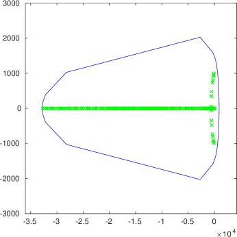
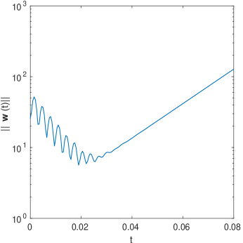
Figure 3: Schnackenberg model. Left plot: Eigenvalues and Field of values of $\widetilde{J}$. Right plot: $\|w\|$ with $w=e^{t\widetilde{J}}w_{0}$.

6.1 Schnakenberg model

The RD-PDE for the Schnakenberg model is given by

$$\begin{cases}u_{t}=\Delta u+\gamma(a-u+u^{2}v),\quad(x,y)\in\Omega=[0,1]\times[0,1],\ t\in]0,T_{f}]\\ v_{t}=d\Delta v+\gamma(b-u^{2}v),\\ (n\nabla u)_{|\partial\Omega}=(n\nabla v)_{|\partial\Omega}=0\\ u(x,y,0)=u_{0}(x,y),v(x,y,0)=v_{0}(x,y)\end{cases}$$ (40)

This model has received great attention in the recent literature (see, e.g., [20, 30]) because in spite of its simplicity, it is representative of classical patterns typically found in biological experiments. The model parameters $a$, $b$, $d$, $\gamma$ are positive constants, and a unique stable equilibrium exists, which undergoes the Turing instability, given by $u_{e}=a+b$, $v_{e}=\frac{b}{(a+b)^{2}}$. We consider the typical values $d=10,\gamma=1000,a=0.1,b=0.9$, yielding a cos-like spotty pattern of the type $\cos(\nu_{x}\pi x)\cos(\nu_{y}\pi y)$ with the selected modes $(\nu_{x},\nu_{y})=(3,5),(5,3)$ [3] (see Figure 4). We consider the initial conditions $u_{0}(x,y)=u_{e}+10^{-5}{\tt rand}(x,y),v_{0}(x,y)=v_{e}+10^{-5}{\tt rand}(x,y)$ where rand is the default Matlab function with fixed seed of the generator (rng(’default’)) at the beginning of each simulation. To numerically confirm the spectral analysis of the previous section, we consider the matrices (see (19))

$$\widetilde{J}=\begin{bmatrix}\tilde{\Delta}&0\\ 0&A\end{bmatrix}+J,\quad\quad J=\gamma\begin{bmatrix}(-1+2u_{e}v_{e}){\mathbb{I}}&u_{e}^{2}{\mathbb{I}}\\ -2u_{e}{\mathbb{I}}&-u_{e}^{2}{\mathbb{I}}\end{bmatrix}.$$

Here ${\mathbb{I}}$ is the matrix of all ones. Note that $J$ has (multiple) eigenvalues $\lambda(J)_{\pm}=\gamma(-0.1\pm 0.99499i)$, while $\lambda(H(J))_{1,2}\in\{-1.0849\gamma,0.88489\gamma\}$. The equilibrium is reactive because the largest eigenvalue of $H(J)$ is positive. For the chosen parameters, the left plot of Figure 3 displays the field of values and eigenvalues of $\widetilde{J}$, from which we can see that the matrix $\widetilde{J}$ is not stable (its largest (real) eigenvalue is about 60), and its symmetric part is not negative definite The right plot of Figure 3 indicates norm divergence of the solution to the linearized problem, $w=e^{t\widetilde{J}}w_{0}$, thus confirming the existence of the reactivity phase in the initial transient regime. This behavior has been observed for instance in population dynamics ODE models in [40], however we are not aware of a similar computational evidence of the reactivity concept for Turing pattern formation. The experimental results in Figure 3 thus support the reactivity analysis in [27, 28] for the numerical treatment of the Schnakenberg model.

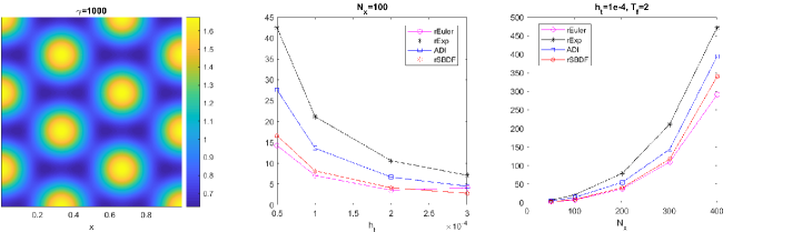
Figure 4: Schnackenberg model. Left plot: Turing pattern solution for $\gamma=1000$ ($N_{x}=400$). Center plot: CPU times (sec) for Test (a), $N_{x}=100$ variation of $h_{t}$. Right plot: CPU times (sec) for Test (b), $h_{t}=10^{-4}$, increasing values of $N_{x}=50,100,200,300,400$.

To study the time dynamics in our simulations we will report the values of the space mean value

$$\langle U_{n}\rangle={\rm mean}(U_{n})\approx\langle u(t_{n})\rangle=\frac{1}{|\Omega|}\int_{\Omega}u(x,y,t_{n})\,dx\,dy\quad\quad t_{n}=n\,h_{t},\quad n=0,\dots,N_{t},$$ (41)

that for $t\rightarrow T_{f}=N_{t}\,h_{t}$ will tend to a constant value, say $\langle U_{n}\rangle\rightarrow{\bar{u}}$, if a stationary pattern is attained. We also report the behavior of the increment $\delta_{n}=\|U_{n+1}-U_{n}\|_{F}$ (Frobenius norm) that will tend to zero if the steady state is reached. These two indicators will be useful also to describe the numerical behaviors of the methods in the initial transient and then to study their reactivity features. Plots with $V_{n}$ show a completely analogous behavior. For the final time $T_{f}=2$ and $N_{y}=N_{x}$, we present the following two tests.

Figure 5: Schnackenberg model- Test (a). Indicators for the rEuler, rExp and ADI methods with $N_{x}=100$ fixed and varying $h_{t}$ in $\{0.5\cdot 10^{4},10^{-4},2\cdot 10^{-4},3\cdot 10^{-4}\}$. We show the time behaviors of the increments $\delta_{n}=\|U_{n+1}-U_{n}\|_{F}$ (upper subfigures) and of the space mean values $<U_{n}>$ (lower subfigures). the zoom insets highlight the reactivity zones ${\cal I}_{1}$ for each method.

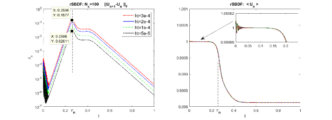
Figure 6: Schnackenberg model- Test (a). Indicators for rSBDF $N_{x}=100$ fixed and varying $h_{t}$ in $\{0.5\cdot 10^{4},10^{-4},2\cdot 10^{-4},3\cdot 10^{-4}\}$. Left plot: time behaviors of the increments $\delta_{n}=\|U_{n+1}-U_{n}\|_{F}$, the reactivity zone ${\cal I}_{1}$ and the stabilizing zone ${\cal I}_{2}$ are separated by the critical time value $\tau_{n}$ . Right plot: space mean values $<U_{n}>$ with zoom inset in the reactivity zone.

Test (a). We fix $N_{x}=100$ and vary $h_{t}$ in $\{0.5\cdot 10^{4},10^{-4},2\cdot 10^{-4},3\cdot 10^{-4}\}$. The simulations reported in Figure 5 for the rEuler, rExp, ADI methods and in Figure 6 for the rSBDF method, show that all methods have a similar qualitative behavior and that two time regimes ${\cal I}_{1}=[0,\tau]$ and ${\cal I}_{2}=]\tau,T_{f}]$ can be distinguished. In ${\cal I}_{1}$ reactivity holds: the oscillating solution departs from the spatially homogeneous pattern due to the superimposed (small random) perturbations and becomes unstable, in ${\cal I}_{2}$ the solution starts to stabilize towards the steady Turing pattern. Numerically the value of $\tau$ can be approximated a-posteriori by $\tau_{n}$, which is the time value where the maximum of the increment $\delta_{n}$ is achieved. Let us discuss in more details the characteristics of the different methods. To this end, the three upper subplots of Figure 5 and the left plot of Figure 6 for rSBDF show the increment $\delta_{n}$ of subsequent approximate solutions as time marches. The three lower subplots of Figure 5 and the right plot of Figure 6 for rSBDF show the behavior of the mean value $<U_{n}>$ as time steps proceed.

${\cal I}_{1}$-reactivity zone. The upper subplots of Figure 5 show that there exists an initial phase of oscillations whose length is method dependent, and for $h_{t}\rightarrow 0$ this length tends to a certain small value $\tau_{0}$. Then for $\tau_{0}\leq t_{n}\leq\tau$ the solution must be unstable, as the necessary condition for Turing instability requires. Comparing with the mean values $<U_{n}>$ curve in the lower subplots of Figure 5, the transfer from ${\cal I}_{1}$ to ${\cal I}_{2}$ corresponds to the steep part of the curve $\langle U(t)\rangle$ that connects the very short-term and the final states of the system; the value of $\tau$ can be related to the inflection point of this curve. In this experiment it is possible to note that $\tau_{0}=\tau_{0}(h_{t}^{p})$ and $\tau=\tau(h_{t}^{p})$. In fact, as also the zoom insets show, for $h_{t}\rightarrow 0$ rEuler and ADI have the same behavior, rExp has curves $<U_{n}>$ with different slopes depending on $h_{t}$. Figure 6 for the rSBDF method emphasizes that this scheme is able to identify the best approximation of $\tau_{0}$ and $\tau$ also for larger value of $h_{t}$, as it could be expected because it is a 2nd order method. The zoom inset shows also that the reactivity oscillations are kept to the minimum amplitude compared to the other schemes.

${\cal I}_{2}$-stabilizing zone. For $h_{t}<h_{t}^{cr}$ all methods reach the asymptotic pattern. Here for $h_{t}^{cr}\simeq 3\cdot 10^{-4}$ rEuler and ADI do not attain any pattern (for clarity, the erratic oscillations of $<U_{n}>$ are only reported in the zooms of Figure 5), while rExp attains the final pattern after a fully oscillating transient behavior (see the (red) oscillations in the central subplots of Figure 5). This value of $h_{t}$ may be interpreted as a critical value for the “reactive stability” of rExp. In the central plot of Figure 4 we report the computational costs of all methods. We recall that by varying $h_{t}$ an increasing number $N_{t}$ of Sylvester matrix equations in (34) of the same dimension need be solved. rEuler and rSBDF have almost the same cost and are cheaper than the other methods. rExp is more expensive than ADI. It is worth noting that the IMEX schemes in vector form are are known to commonly be more expensive than the ADI method for this problem (see e.g. [32]).

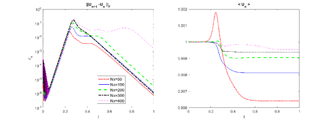
Figure 7: Schnackenberg model-Test (b), for rSBDF with $h_{t}=1$e-4 and increasing values of $N_{x}=50,100,200,300,400$. Left: Increment $\delta_{n}=\|U_{n+1}-U_{n}\|_{F}$. Right: Space mean value $<U_{n}>$.

Test (b): We fix $h_{t}=10^{-4}$ and vary $N_{x}=50,100,200,300,400$, such that the matrix methods solve the same number $N_{t}$ of Sylvester equations of increasing sizes. As a sample, results for rSBDF are reported in Figure 7. All other methods have a similar time dynamics behavior. The right plot shows that the final value of $<U_{n}>$, that is $\bar{u}=\bar{u}(N_{x})$, changes with $N_{x}$, as expected. The left plot seems to indicate that $\tau=\tau(h_{t},N_{x})$ is an increasing function of $N_{x}$. This might be related to the fact the (discrete) initial conditions $U_{0},V_{0}$ have different sizes and include different (though small) random perturbations. This sensitivity with respect to the initial conditions is well known in the pattern formation literature (see, e.g., [22]) and it goes under the name of robustness problem. This is the main reason why we do not propose to apply low rank approximation methods for (34) (see, e.g., [25] for the differential Lyapunov and Riccati matrix equations). In fact, it can be shown that projecting the Turing solution on a low-rank manifold, especially during the transient unstable time dynamics, can induce the selection of specific Fourier modes in the final pattern (see the discussion above). This topic will be object of future investigations. The right plot of Figure 4 reports the computational costs of all methods. We recall that by varying $N_{x}$, Sylvester matrix equations in (34) of increasing size are solved by the reduced spectral approach. As in Test (a), rEuler and rSBDF have almost the same cost and are cheaper than the other methods and ADI is less expensive than rExp. For the largest spatial dimensions rEuler becomes the most effective, costs-wise. We stress that for the larger values of $N_{x}$ this test could not be performed by classical vector-oriented version of the same schemes due to the high computational load.

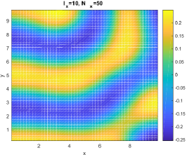
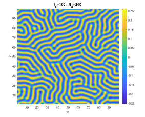
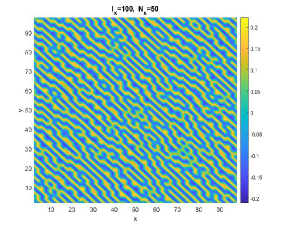
Figure 8: Labyrinth Turing pattern of DIB Model. Top left: $\Omega=[0,10]\times[0,10]$ and $N_{x}=50(h_{x}=0.2)$. Top right: $\Omega=[0,100]\times[0,100]$ and $N_{x}=200$ $(h_{x}=0.5)$. Bottom: $\Omega=[0,100]\times[0,100]$ and $N_{x}=50$ $(h_{x}=2)$.

6.2 DIB model

In this section we report on the importance of the matrix-oriented approach to carefully approximate the spatial structure of Turing patterns on fine meshgrids and large domains at feasible computational costs.

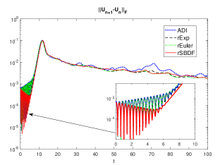
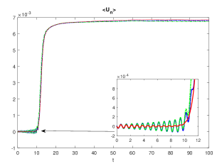
Figure 9: DIB model: time dynamics of the increment $\delta_{n}=\|U_{n+1}-U_{n}\|_{F}$ (left plot) and of the mean value $<U_{n}>$ (right plot) for all methods in the case $\Omega=[0,100]\times[0,100]$, $T_{f}=100$, $h_{t}=10^{-2}$, $N_{x}=200$.

Towards this aim we consider the RD-PDE model studied in [18, 33] describing an electrodeposition process for metal growth where the kinetics in (33) are given by

$$\begin{split}&f_{1}(u,v)=\rho\left(A_{1}(1-v)u-A_{2}\,u^{3}-B(v-\alpha)\right),\\ &f_{2}(u,v)=\rho\left(C(1+k_{2}u)(1-v)[1-\gamma(1-v)]-Dv(1+k_{3}u)(1+\gamma v))\right).\end{split}$$ (42)

Here $u(x,y,t)$ represents the morphology of the metal deposit, while $v(x,y,t)$ monitors its surface percentual chemical composition. The nonlinear source terms account for generation and loss of relevant material during the process. In [17] this model has been proposed to study pattern formation during the charge-discharge process of batteries. In the same article, it has also been proved that for a given parameter choice of the RD-PDE model there exists an intrinsic pattern type that can only emerge if an effective domain size of integration is considered, and this is given by ${\cal A}=\rho|\Omega|$, where $|\Omega|$ = area($\Omega$). Hence, if the scaling factor in (42) is $\rho=1$, a large domain $\Omega$ must be chosen to “see” the Turing pattern, and the grid fineness sufficiently high to capture the pattern details. For this reason, the number of meshpoints $N_{x},N_{y}$, that is the size of the Sylvester equations (34), must be sufficiently large. Figure 8 reports three typical situations: the upper left plot refers to a too small domain to be able to identify the morphological class, which is instead clearly visible in the upper right plot, determined with a much larger domain and a fine grid. In the third setting (large domain but a too coarse grid, $N_{x}=50$) shown in the lower plot of Figure 8, the numerical approximation is unable to clearly detect the labyrinth pattern in its full granularity. These solutions have been obtained by solving (33)-(42) on a square domain $\Omega=[0,\ell_{x}]\times[0,\ell_{x}]$ and with the following parameter choice for which a labyrinth pattern is expected ([17, 18, 33]):

$$d_{1}=1,d_{2}=20,\rho=1,A_{1}=10,A_{2}=30,k_{2}=2.5,k_{3}=1.5,\alpha=0.5,\gamma=0.2,D=2.4545,B=66,C=3.$$

We have applied ADI and the matrix methods rEuler, rExp, rSBDF until $T_{f}=100$, with $h_{t}=10^{-2}$. In Figure 9 we show the dynamics of the increment $\delta_{n}$ and of the mean value $<U_{n}>$ for the simulations corresponding to the full labyrinth in Figure 8(upper right). For the chosen (large) $h_{t}$ the methods exhibit different reactivity and stabilizing properties. The rSBDF method seems to display the best performance.

Methods	$\ell_{x}=10,N_{x}=50$	$\ell_{x}=100,N_{x}=200$	$\ell_{x}=100,N_{x}=300$
IMEX Euler (vector form)	3.5742	90.2079	234.7923
rEuler	2.1592	34.3328	79.6804
rSBDF	3.3318	51.1874	118.4675
rExp	4.6030	50.6238	127.8123
ADI	3.2780	44.3830	95.0798

Table 2: DIB model. Computational times in seconds for all methods to obtain the two top patterns in Figure 8. The cost for the case $N_{x}=300,\ell_{x}=100$ is also reported.

Table 2 reports the computational times of all numerical methods for obtaining the patterns in Figure 8, that is for the two cases (i) $N_{x}=50,\ell_{x}=10,$ (left) and (ii) $N_{x}=200,\ell_{x}=100$ (right), including that of the IMEX Euler vector formulation (implemented similarly to that used in Table 1). The cost for a larger spatial meshgrid $N_{x}=300$ on $\Omega=[0,100]\times[0,100]$ is also reported. For $N_{x}=50$, that is when the pattern is not well identified, all methods display similar computational performances. In the other cases, the vector form significantly suffers from dealing with much larger dimensional data, with respect to the matrix-oriented schemes. rEuler exhibits the best computational times for all dimensions, requiring about one third of the other methods’ time for the large values of $N_{x}$. The other matrix-based schemes are almost equivalent, with ADI being slightly less expensive. These preliminary experiments seem to indicate that the matrix formulation is a competitive methodology for the numerical solution of the RD-PDE systems when a fine spatial grid is necessary to capture the morphological features of the pattern.

7 Conclusions

By exploiting the Kronecker structure of the diffusion matrix, we have shown that the classical semi-discretization in space of reaction-diffusion PDEs on regular domains can be seen as a system of matrix ODE equations (see (6)). ODE solvers in time such as IMEX Euler, 2SBDF schemes and the Exponential Euler method, can thus be implemented in matrix form, requiring a sequence of small matrix problems (Sylvester equations, matrix exponentials) to be solved at each time step. Due to the modest size of these matrices, the computational cost per iteration can be made lower than that of the corresponding vector approaches, by working in the (reduced) spectral space. To avoid the high computational load of the vector-IMEX methods, in the literature this challenge has often been faced by the using ADI approach; our comparisons show that the new reduced schemes can be a valid alternative to ADI. In particular, rEuler exhibits the best performance. To the best of our knowledge, the exponential method rExp is new in this field of application. The improvement obtained by working with matrix ODEs allows us to capture the key features of Turing pattern solutions, and this has been shown by using two typical benchmarks, the Schnackenberg and DIB models. We plan to deepen our understanding of matrix-oriented formulation by further exploring higher order methods so as to improve the accuracy of the methods while maintaining efficiency. Finally, we speculate that the matrix-approach can be particularly helpful, for instance, in the context of parameter identification problems (see e.g. [33]) to significantly reduce the computational load for the corresponding constrained minimization problem, which requires the approximations of PDE models at each optimization step.

Appendix: Matlab code

This Appendix reports the possible implementation in Matlab ([24]) of the reduced Euler Algorithm and of the reduced Exponential Euler Algorithm for a RD-PDE system of two equations. The displayed codes compute and employ explicit inverse matrices. This procedure turned out to be more effective than solving the corresponding systems on the fly at each iteration. We also note that the reported rEuler code explicitly computes the eigenvalue decomposition of $A_{1},A_{2}$ and $B$, which could be avoided: in rExp we showed how to derive the eigendecompositions of all matrices from that of $T$.

%%% INPUT:
% F1, F2 = kinetics of the RD-model (inputs to be edited as needed)
% T  = Approximation of the 1D laplacian, order p, of size Nx-1
% Lx = length of spatial domain: [0,Lx]x[0,Lx]
% Nx = number of points for the spatial discretization in each direction
% Tf = final time of integration
% ht = time step
% p = order of approximation of the second derivative
% par = parameters structure for the RD-model
% w = correction coefficient (only for rExp)

%%% OUPUT:
% U, V = solution of the models
%%%%%%%%%%%%%%%%%%%%%%%%%%%%%%%%%%%%%%%%%%%%%%%% rEuler
function [U,V]=rEuler(F1, F2, T, Lx, Nx, Tf, ht, p, ue, ve, d, par)
hs = Lx/(Nx);
I = eye(Nx-1);
Nt = Tf/ht;
A1 = I-ht*T;             A2=I-d*ht*T;
[Qa1,Ra1] = eig(A1);     [Qa2,Ra2] = eig(A2);
I_Qa1 = inv(Qa1);        I_Qa2 = inv(Qa2);
B = -ht*T’;            [Qb,Rb]=eig(B);
                       I_Qb = inv(Qb);
dA1 = diag(Ra1); dA2 = diag(Ra2); dB = diag(Rb);
Inveig_u = 1./(dA1*ones(1,Nx-1) + ones(Nx-1,1)*dB’);
Inveig_v = 1./(dA2*ones(1,Nx-1) + ones(Nx-1,1)*d*dB’);
rng(’default’);
Rs = rand(Nx-1); %perturbation matrix for the IC
U = ue+Rs*1e-05;
V = ve+Rs*1e-05;
for k=1:Nt
     C_u = U+ht*F1(U, V, par);
     C_v = V+ht*F2(U, V, par);
     Cc_u = I_Qa1*C_u*Qb;
     Cc_v = I_Qa2*C_v*Qb;
     Xx = Cc_u.*Inveig_u;
     Yy = Cc_v.*Inveig_v;
     U = Qa1*Xx*I_Qb;
     V = Qa2*Yy*I_Qb;
end

%%%%%%%%%%%%%%%%%%%%%%%%%%%%%%%%%%%%%%%%%%%%%%%% rExp
function [U,V]=rExp(F1, F2, T, Lx, Nx, Tf, ht, p, ue, ve, d, par, w)
hs = Lx/(Nx);
I = eye(Nx-1);
Nt = Tf/ht;
rng(’default’);
Rs = rand(Nx-1); %perturbation matrix for the IC
U1 = ue+Rs*1e-05;
V1 = ve+Rs*1e-05;

[QT,ET]=eig(T);
A1plus = T-w*I;
Q1plus = QT;       I_Q1plus = inv(QT);      E1plus = ET-w*I;
Bplus = T’;
QBplus = inv(QT’); I_QBplus = QT’;          EBplus = conj(ET);
A2plus = d*T - w*I;
Q2plus = QT;       I_Q2plus = inv(Q2plus);  E2plus = d*ET-w*I;
EAB1 = exp(ht*diag(E1plus))*exp(ht*diag(EBplus).’);
EAB2 = exp(ht*diag(E2plus))*exp(ht*d*diag(EBplus).’);
LL1 = 1./(ht*diag(E1plus)*ones(1,Nx-1)+ht*ones(Nx-1,1)*diag(EBplus).’);
LL2 = 1./(ht*diag(E2plus)*ones(1,Nx-1)+ht*d*ones(Nx-1,1)*diag(EBplus).’);
U1eig = Q1plus\U1*QBplus;
V1eig = Q2plus\V1*QBplus;
for k=1:Nt
    G1 = F1(U1,V1, par) + w*U1;
    ProjG1 = I_Q1plus*G1*QBplus;
    ErhsU = EAB1.*ProjG1-ProjG1;
    U = EAB1.*(U1eig)+ ht*(LL1.*ErhsU);
    U1eig = U;
    U = Q1plus*U*I_QBplus;

    G2 = F2(U1,V1, par)+w*V1;
    ProjG2 = I_Q2plus*G2*QBplus;
    ErhsV = EAB2.*ProjG2-ProjG2;
    V = EAB2.*V1eig + ht*(LL2.*ErhsV);
    V1eig = V;
    V = Q2plus*V*I_QBplus;
    U1 = U; V1 = V;
end

References

- [1] P. Amodio, I. Sgura, High order finite difference schemes for the solution of second order BVPs, J. Comput. Appl. Math. A 176(1) (2005) 59-76. DOI: doi.org/10.1016/j.cam.2004.07.008
- [2] U. M. Ascher, S. J. Ruuth, B. T. R. Wetton, Implicit-explicit methods for time dependent PDE’s. SIAM J. Numerical Analysis 32(3) (1995) 797-823.
- [3] C. H. L. Beentjes, Pattern formation analysis in the Schnakenberg model. Technical Report, University of Oxford, Oxford, UK (2015).
- [4] M. Behr, P. Benner, J. Heiland, Solution Formulas for Differential Sylvester and Lyapunov Equations (2018). arXiv preprint, arXiv:1811.08327
- [5] B. Benner, N. Lang, Peer Methods for the Solution of Large-Scale Differential Matrix Equations (2018). arXiv preprint, arXiv:1807.08524.
- [6] B. Bozzini, G. Gambino et. al, Weakly nonlinear analysis of Turing patterns in a morphochemical model for metal growth, Comp. & Math. App. 70(8) (2015) 1948-1969. DOI: 10.1016/j.camwa.2015.08.019
- [7] T. Breiten, V. Simoncini, M. Stoll, Low-rank solvers for fractional differential equations, Electronic Transactions on Numerical Analysis 45 (2016) 107-132. DOI: 10.17617/2.2270973
- [8] A. De Wit, Spatial pattern and spatiotemporal dynamics in chemical systems, Adv. chem. Phys, 10 (1999) 435-513. DOI: https://doi.org/10.1002/9780470141687.ch5
- [9] H. Föll, J. Carstensen, Pattern formation during anodic etching of semiconductors, ECS Transactions, 33(20) (2011) 11-28. DOI: 10.1149/1.3563752
- [10] J. Frank, W. Hundsdorfer, J.G. Verwer, On the stability of implicit-explicit linear multistep methods, Appl. Numer. Math. 25 (1997) 193-205. DOI: doi.org/10.1016/S0168-9274(97)00059-7
- [11] M. Frittelli, A. Madzvamuse, I.Sgura, C. Venkataraman, Lumped finite elements for reaction–cross-diffusion systems on stationary surfaces, Computers and Mathematics with Applications, 74 (12) (2017) 3008-3023. DOI:doi.org/10.1016/j.camwa.2017.07.044
- [12] M. Frittelli, A. Madzvamuse, I.Sgura, C. Venkataraman, Numerical Preservation of Velocity Induced Invariant Regions for Reaction–Diffusion Systems on Evolving Surfaces, Journal of Scientific Computing 77(2) (2018) 971-1000. DOI: doi.org/10.1007/s10915-018-0741-7
- [13] U. Z. George, A. Stephanou and A. Madzvamuse, Mathematical modelling and numerical simulations of actin dynamics in the eukaryotic cell, Journal of Mathematical Biology 66(3) (2013) 547-593. DOI: 10.1007/s00285-012-0521-1
- [14] A. Gerisch, M.A.J. Chaplain, Robust numerical methods for taxis–diffusion–reaction systems: applications to biomedical problems, Math. Comp. Mod. 43 (2006) 49-75. http://dx.doi.org/10.1016/j.mcm.2004.05.016.
- [15] M. Hochbruck and A. Ostermann, Exponential integrators, Acta Numerica 19 (2010). 209-286. DOI: doi.org/10.1017/S0962492910000048
- [16] P. M. Knupp and S. Steinberg, The fundamental of grid generation, Knupp, 1992.
- [17] D. Lacitignola, B. Bozzini, M. Frittelli, I. Sgura, Turing pattern formation on the sphere for a morphochemical reaction-diffusion model for electrodeposition, Commun Nonlinear Sci Numer Simulat 48 (2017) 484-508. DOI: 10.1016/j.cnsns.2017.01.008
- [18] D. Lacitignola, B. Bozzini, I. Sgura, Spatio-temporal organization in a morphochemical electrodeposition model: Hopf and Turing instabilities and their interplay, European Journal of Applied Mathematics 26(2) (2015) 143-173. DOI: doi.org/10.1017/S0956792514000370
- [19] M. G. Larson, F. Bengzon, The Finite Element Method: Theory, Implementation, and Practice, Springer, 2010.
- [20] P. Liu, J. Shi, Y. Wang and X. Feng, Bifurcation analysis of reaction-diffusion Schakenberg model J Math Chem 51 (2013) 2001-2019. DOI: 10.1007/s10910-013-0196-x
- [21] A. Madzvamuse, A.J. Wathen, P.K. Maini, A moving grid finite element method applied to a model biological pattern generator, J. Comput. Phys. 190(2) (2003) 478–500. DOI: 10.1016/S0021-9991(03)00294-8
- [22] P. Maini, H. Othmer, Mathematical Models for Biological Pattern Formation, The IMA Volumes in Mathematics and its Applications - Frontiers in application of Mathematics, Springer-Verlag, New York, 2001.
- [23] H. Malchow, S. Petrowski, E. Venturino, Spatio temporal Patterns in Ecology and Epidemiology, Chapman & Hall, U.K., 2008.
- [24] The MathWorks, Inc., MATLAB 9.4, R2018a ed., 2018.
- [25] H. Mena, A. Ostermann, L. M. Pfurtscheller, C. Piazzola, Numerical low-rank approximation of matrix differential equations, J. Comp.Applied Mathematics 340 (2018) 602–614. DOI: https://doi.org/10.1016/j.cam.2018.01.035
- [26] J. Murray, Mathematical Biology II - Spatial Models and Biomedical Applications, Spinger-Verlag, Berlin Heidelberg, 2003.
- [27] M.G. Neubert, H. Caswell, Alternatives to resilience for measuring the responses of ecological systems to perturbations, Ecology 78 (1997) 653. DOI: https://doi.org/10.1890/0012-9658(1997)078[0653:ATRFMT]2.0.CO;2
- [28] M.G. Neubert, H. Caswell, J.D. Murray, Transient dynamics and pattern formation: reactivity is necessary for Turing instabilities, Math. Biosciences 175 (2002) 1-11. DOI: 10.1016/S0025-5564(01)00087-6
- [29] D. Palitta, V. Simoncini, Matrix-equation-based strategies for convection-diffusion equations, BIT Numer Math 56 (2016) 751-776. DOI: 10.1007/s10543-015-0575-8
- [30] M. R. Ricard and S. Mischler, Turing instabilities af Hopf bifurcation, J Nonlinear Sci 19 (2009) 476-496. DOI: https://doi.org/10.1007/s00332-009-9041-6
- [31] J. Ruuth, Implicit-explicit methods for reaction-diffusion problems in pattern formation, J. Math. Biol. 34 (1995) 148-176. DOI: https://doi.org/10.1007/BF00178771
- [32] G. Settanni, I. Sgura, Devising efficient numerical methods for oscillating patterns in reaction-diffusion system, Journal of Computational and Applied Mathematics, 292 (2016) 674-693. DOI: 10.1016/j.cam.2015.04.044
- [33] I. Sgura, A.S. Lawless, B. Bozzini, Parameter estimation for a morphochemical reaction-diffusion model of electrochemical pattern formation, Inverse Problems in Science and Engineering, 27 (5), (2019) 618-647, DOI: 10.1080/17415977.2018.1490278
- [34] I. Sgura, B. Bozzini, D. Lacitignola, Numerical approximation of Turing patterns in electrodeposition by ADI methods, J. Comput. Appl. Math. 236(16) (2012) 4132-4147. DOI: 10.1016/j.cam.2012.03.013
- [35] J. A. Sherratt, Turing pattern in desert, in S.B. Cooper, A. Dawar (Eds.) How the World Computes, Lecture Notes in Computer Science 7318, Springer, New York, 2012.
- [36] J. A. Sherratt, M. A.J. Chaplain, A new mathematical model for avascular tumour growth, J. Math. Biol. 43 (2001) 291–312. DOI: https://doi.org/10.1007/s002850100088
- [37] V. Simoncini, A new iterative method for solving large-scale Lyapunov matrix equations, SIAM J. Sci. Comput. 29(3) (2007) 1268-1288. DOI: https://doi.org/10.1137/06066120X
- [38] V. Simoncini, Computational methods for linear matrix equations. SIAM Review, 58(3) (2016) 377–441. DOI: https://doi.org/10.1137/130912839
- [39] T. Stillfjord, Low-rank second-order splitting of large-scale differential Riccati equations, IEEETransactions on Automatic Control, 60(10) (2015) 2791-2796. DOI: 10.1109/TAC.2015.2398889
- [40] L.N. Trefethen and M. Embree. Spectra and pseudospectra. The behavior of non-normal matrices and operators. Princeton University Press (2005).
- [41] A. M. Turing, The chemical bases of morphogenesis, Phil. Trans. Royal Soc. London B 237 (1952) 37-72. DOI: https://doi.org/10.1098/rstb.1952.0012
- [42] V. K. Vanag, Waves and pattern in reaction-diffusion systems. Belousov-Zhabotinsky reaction in water-in-oil microemulsions, Phys.-Uspekhi 47(9) (2004) 923-941. DOI: https://doi.org/10.1070/PU2004v047n09ABEH001742