Bit-Interleaved Coded Multiple Beamforming in Millimeter-Wave Massive MIMO Systems

Sadjad Sedighi CPCC, Dept of EECS, UC Irvine, Irvine, CA, USA, Ender Ayanoglu CPCC, Dept of EECS, UC Irvine, Irvine, CA, USA,
Abstract

In this paper we carry out the asymptotic diversity analysis for millimeter-wave (mmWave) massive multiple-input multiple-output (MIMO) systems by using bit interleaved coded multiple beamforming (BICMB). First, a single-user mmWave system which employs $M_{t}$ antenna subarrays at the transmitter and $M_{r}$ antenna subarrays at the receiver is studied. Each antenna subarray in the transmitter and the receiver has $N_{r}$ and $N_{t}$ antennas, respectively. We establish a theorem for the diversity gain when the number of antennas in each remote antenna unit (RAU) goes to infinity. Based on the theorem, the distributed system with BICMB achieves full spatial multiplexing of $L_{t}=\sum_{i,j}L_{ij}$ and full spatial diversity of $\frac{\left(\sum_{i,j}\beta_{ij}\right)^{2}}{\sum_{i,j}\beta_{ij}^{2}L_{ij}^{-1}}$ where $L_{ij}$ is the number of propagation paths and $\beta_{ij}$ is the large scale fading coefficient between the $i$th RAU in the transmitter and the $j$th RAU in the receiver. This result shows that one can increase the diversity gain in the system by increasing the number of RAUs. Simulation results show that, when the perfect channel state information assumption is satisfied, the use of BICMB increases the diversity gain in the system.

This work was partially supported by NSF under Grant No. 1547155.

1 Introduction

After the need for a new generation for mobile systems to handle tens of billions of wireless devices, millimeter-wave (mmWave) communication became an important candidate for Fifth Generation (5G) mobile communication systems [1, 2, 3]. The mmWave signals face severe penetration loss and path loss compared to signals in current cellular systems (3G or LTE) [4]. One of the advantages of the mmWave frequencies is that they enable us to pack more antennas in the same area compared to a lower range of frequencies.111Although strictly speaking, mmWave corresponds to the range 30-300 GHz, in practical use, about 5-6 to 100 GHz may be termed mmWave frequencies. This leads to highly directional beamforming and large-scale spatial multiplexing in mmWave frequencies. By exploiting these properties, massive MIMO systems can be developed. The principles of beamforming are independent of the carrier frequency, but it is not practical to use fully digital beamforming schemes for massive MIMO systems [5, 6, 7, 8]. Power consumption and cost perspectives are the main obstacles due to the high number of radio frequency (RF) chains required for the fully digital beamforming, i.e., one RF chain per antenna element [9]. To address this problem, hybrid analog-digital processing of the precoder and combiner for mmWave communications systems is being considered [10, 11, 12, 13, 14, 15].

Bit-interleaved coded modulation (BICM) was introduced as a way to increase the code diversity [16, 17]. As stated in [18], bit-interleaved coded multiple beamforming (BICMB) has a great impact on the diversity gain performance of a MIMO system. Recently, by comparing the diversity gain in both co-located and distributed systems the authors of [19] have shown that increasing the number of RAUs in the distributed system does increase the diversity gain and/or multiplexing gain. In Section II and III, BICMB is analyzed. We show that by using BICM in the system, one can achieve full spatial multiplexing without any loss in the diversity gain. That is, in Section III, we show that BICMB achieves full diversity order of $M_{r}M_{t}L$ and full spatial diversity of $M_{r}M_{t}L$ in a special case when the number of propagation paths is constant for all paths between RAUs, i.e., $L_{ij}=L$ over a limited scattering mmWave channel. We provide design criteria for the interleaver that guarantee full diversity and full spatial multiplexing.

We would like to reiterate that the asymptotical diversity analysis obtained in this paper is under the idealistic assumption of having perfect channel state information both at the transmitter and the receiver as done in similar works.

Notation: Boldface upper and lower case letters denote matrices and column vectors, respectively. The minimum Hamming distance of a convolutional code is defined as $d_{\text{free}}$. The symbol Nssubscript๐‘๐‘ N_{s} denotes the total number of symbols transmitted at a time. The minimum Euclidean distance between the two constellation points is given by $d_{\text{min}}$. The superscripts $(.)^{H},(.)^{T},(.)^{*},(\bar{.})$ and the symbol $\forall$ denote the Hermitian, transpose, complex conjugate, binary complement, and for all, respectively. $\mathcal{CN}(0,1)$ denotes a circularly symmetric complex Gaussian random variable with zero mean and unit variance. The expectation operator is denoted by $E\left[.\right]$. Also, $[\mathbf{A}]_{ij}$ gives the $(i,j)$th entry of matrix $\mathbf{A}$. Finally, diag$\{a_{1},a_{2},\dots,a_{N}\}$ stands for a diagonal matrix with diagonal elements $\{a_{1},a_{2},\dots,a_{N}\}$.

2 System Model

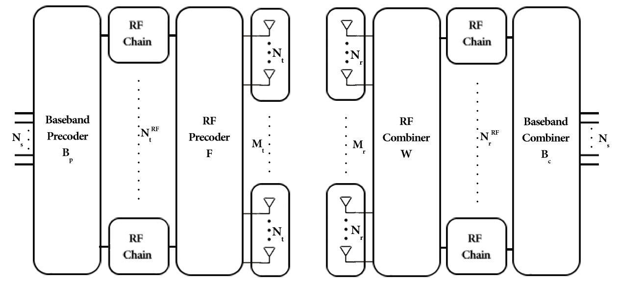
Consider a single-user mmWave massive MIMO system as shown in Fig. 1. In this system, the transmitter sends Nssubscript๐‘๐‘ N_{s} data streams to a receiver. The transmitter is equipped with $N_{t}^{RF}$ RF chains and $M_{t}$ RAUs, where each RAU has $N_{t}$ antennas, while at the receiver, the number of RF chains and RAUs is given by $N_{r}^{RF}$ and $M_{r}$, respectively. Each RAU at the receiver has $N_{r}$ antennas. When $M_{t}=M_{r}=1$, the system reduces to a conventional co-located MIMO (C-MIMO) system.

Refer to caption
Figure 1: Block diagram of a mmWave massive MIMO system with distributed antenna arrays.

The input to the system is Nssubscript๐‘๐‘ N_{s} data streams. The vector of data symbols to be transmitted by the transmitter at each time instant, ๐ฑโˆˆโ„‚Nsร—1๐ฑsuperscriptโ„‚subscript๐‘๐‘ 1\mathbf{x}\in\mathbb{C}^{N_{s}\times 1}, can be expressed as

๐ฑ=[x1,โ€ฆ,xNs]T,๐ฑsuperscriptsubscript๐‘ฅ1โ€ฆsubscript๐‘ฅsubscript๐‘๐‘ ๐‘‡\displaystyle\mathbf{x}=\left[x_{1},...,x_{N_{s}}\right]^{T}, (1)

where Eโ€‹[๐ฑ๐ฑH]=๐ˆNs๐ธdelimited-[]superscript๐ฑ๐ฑ๐ปsubscript๐ˆsubscript๐‘๐‘ E\left[\mathbf{x}\mathbf{x}^{H}\right]=\mathbf{I}_{N_{s}}. The preprocessing at the baseband is applied by means of the matrix ๐pโˆˆโ„‚NtRโ€‹Fร—Nssubscript๐๐‘superscriptโ„‚superscriptsubscript๐‘๐‘ก๐‘…๐นsubscript๐‘๐‘ \mathbf{B}_{p}\in\mathbb{C}^{N_{t}^{RF}\times N_{s}}. The last stage of data preprocessing is performed at RF, when beamforming is applied by means of phase shifters and combiners. A set of $M_{t}N_{t}$ phase shifters is applied to the output of each RF chain. As a result of this process, different beams are formed in order to transmit the RF signals. We can model this process with an $M_{t}N_{t}\times N_{t}^{RF}$ complex matrix $\mathbf{F}$. Note that the baseband precoder $\mathbf{B}_{p}$ modifies both amplitude and phases, while only phase changes can be realized by $\mathbf{F}$ since it is implemented by using analog phase shifters.

We assume a narrowband flat fading channel model and obtain the received signal as

$\displaystyle\mathbf{z}=\mathbf{HF}\mathbf{B}_{p}\mathbf{x}+\mathbf{n},$ (2)

where $\mathbf{H}$ is an $M_{r}N_{r}\times M_{t}N_{t}$ channel matrix with complex-valued entries and $\mathbf{n}$ is an $M_{r}N_{r}\times 1$ vector consisting of i.i.d. $\mathcal{CN}(0,N_{0})$ noise samples, where $N_{0}=\frac{N_{t}}{SNR}$. The processed signal is given by

$\displaystyle\mathbf{y}=\mathbf{B}_{c}^{H}\mathbf{W}^{H}\mathbf{HF}\mathbf{B}_{p}\mathbf{x}+\mathbf{B}_{c}^{H}\mathbf{W}^{H}\mathbf{n},$ (3)

where $\mathbf{W}$ is the $M_{r}N_{r}\times N_{r}^{RF}$ RF combining matrix, and $\mathbf{B}_{c}$ is the Nr(rโ€‹f)ร—Nssuperscriptsubscript๐‘๐‘Ÿ๐‘Ÿ๐‘“subscript๐‘๐‘ N_{r}^{(rf)}\times N_{s} baseband combining matrix.

The channel matrix $\mathbf{H}$ can also be written as

$\displaystyle\mathbf{H}=\begin{bmatrix}\sqrt{\beta_{11}}\mathbf{H}_{11}&\dots&\sqrt{\beta_{1M_{t}}}\mathbf{H}_{1M_{t}}\\ \vdots&\ddots&\vdots\\ \sqrt{\beta_{M_{r}1}}\mathbf{H}_{M_{r}1}&\dots&\sqrt{\beta_{M_{r}M_{t}}}\mathbf{H}_{M_{r}M_{t}}\end{bmatrix},$ (4)

where $\beta_{ij}$, a real-valued nonnegative number, represents the large-scale fading effect between the $i$th RAU at the receiver and $j$th RAU at the transmitter. The normalized subchannel matrix $\mathbf{H}_{ij}$ is the MIMO channel between the $i$th RAU at the receiver and the $j$th RAU at the transmitter.

Analytical channel models such as Rayleigh fading are not suitable for mmWave channel modeling. The reason for this is the fact that the scattering levels represented by these models are too rich for mmWave channels[11]. In this paper, the model is based on the Saleh-Valenzuela model that is often used in mmWave channel modeling [20] and standardization [21]. For simplicity, each scattering cluster is assumed to contribute a single propagation path. The subchannel matrix $\mathbf{H}_{ij}$ is given by

$\displaystyle\mathbf{H}_{ij}=\sqrt{\frac{N_{t}N_{r}}{L_{ij}}}\sum_{l=1}^{L_{ij}}\alpha_{ij}^{l}\mathbf{a}_{r}(\theta_{ij}^{l})\mathbf{a}_{t}^{H}(\phi_{ij}^{l}),$ (5)

where $L_{ij}$ is the number of propagation paths and $\alpha_{ij}^{l}$ is the complex-gain of the $l$th ray which follows $\mathcal{CN}(0,1)$, the vectors $\mathbf{a}_{r}(\theta_{ij}^{l})$ and $\mathbf{a}_{t}(\phi_{ij}^{l})$ are the normalized receive/transmit array response and $\theta_{ij}^{l}$ and $\phi_{ij}^{l}$ are its random azimuth angles of arrival and departure respectively. The elevation dimension is ignored.

The uniform linear array (ULA) is employed by the transmitter and receiver in our study. For an $N$-element ULA, the array response vector can be given by

๐šUโ€‹Lโ€‹Aโ€‹(ฯ•)=1Nโ€‹[1,ejโ€‹2โ€‹ฯ€ฮปโ€‹dโ€‹sโ€‹iโ€‹nโ€‹(ฯ•),โ€ฆ,ejโ€‹(Nโˆ’1)โ€‹2โ€‹ฯ€ฮปโ€‹dโ€‹sโ€‹iโ€‹nโ€‹(ฯ•)]T,subscript๐š๐‘ˆ๐ฟ๐ดitalic-ฯ•1๐‘superscript1superscript๐‘’๐‘—2๐œ‹๐œ†๐‘‘๐‘ ๐‘–๐‘›italic-ฯ•โ€ฆsuperscript๐‘’๐‘—๐‘12๐œ‹๐œ†๐‘‘๐‘ ๐‘–๐‘›italic-ฯ•๐‘‡\displaystyle\mathbf{a}_{ULA}(\phi)=\frac{1}{\sqrt{N}}\left[1,e^{j\frac{2\pi}{\lambda}dsin(\phi)},\dots,e^{j(N-1)\frac{2\pi}{\lambda}dsin(\phi)}\right]^{T}, (6)

where $\lambda$ is the wavelength of the carrier, and $d$ is the distance between neighboring antenna elements.

We leverage both BICM and multiple beamforming to form BICMB. An interleaver is used to interleave the output bits of a binary convolutional encoder. Then the output of the interleaver is mapped over a signal set $\chi\subset\mathbb{C}$ of size $|\chi|=2^{m}$ with a binary labeling map $\mu:\{0,1\}^{m}\rightarrow\chi$. The interleaver design has two criteria[18]:

  1. 1.

    Consecutive coded bits are mapped over different symbols,

  2. 2.

    each subchannel should be utilized at least once within $d_{\text{free}}$ distinct bits among different codewords by using proper code and interleaver.

Note that the free distance $d_{\text{free}}$ of the convolutional encoder should satisfy dfreeโ‰ฅNssubscript๐‘‘freesubscript๐‘๐‘ d_{\text{free}}\geq N_{s}.

For mapping the bits onto symbols, Gray encoding is used. Also, we are using a Viterbi decoder at the receiver. The interleaver $\pi$ is used to interleave the code sequence $\underline{c}$. Then the output of the interleaver is mapped onto the signal sequence $\underline{x}\in\chi$.

The only beamforming constraint here is a total power constraint, because one can control both the amplitude and the phase of a signal. As we know the total power constraint leads to a simple solution based on SVD [11]

$\displaystyle\mathbf{H}=\mathbf{U\Lambda V}^{H}=\left[\mathbf{u}_{1}\mathbf{u}_{2}\dots\mathbf{u}_{M_{r}N_{r}}\right]^{H}\mathbf{H}\left[\mathbf{v}_{1}\mathbf{v}_{2}\dots\mathbf{v}_{M_{t}N_{t}}\right],$ (7)

where $\mathbf{U}$ and $\mathbf{V}$ are $M_{r}N_{r}\times M_{r}N_{r}$ and $M_{t}N_{t}\times M_{t}N_{t}$ unitary matrices, respectively, and $\mathbf{\Lambda}$ is an $M_{r}N_{r}\times M_{t}N_{t}$ diagonal matrix with singular values of $\mathbf{H}$, $\lambda_{i}\in\mathbb{R}$, on the main diagonal with decreasing order. By exploiting the optimal precoder and combiner, the system input-output relation in (3) at the $k$th time instant can be written as

๐ฒk=[๐ฎ1โ€‹๐ฎ2โ€‹โ€ฆโ€‹๐ฎNs]Hโ€‹๐‡โ€‹[๐ฏ1โ€‹๐ฏ2โ€‹โ€ฆโ€‹๐ฏNs]โ€‹๐ฑ+[๐ฎ1โ€‹๐ฎ2โ€‹โ€ฆโ€‹๐ฎNs]Hโ€‹๐งk,subscript๐ฒ๐‘˜superscriptdelimited-[]subscript๐ฎ1subscript๐ฎ2โ€ฆsubscript๐ฎsubscript๐‘๐‘ ๐ป๐‡delimited-[]subscript๐ฏ1subscript๐ฏ2โ€ฆsubscript๐ฏsubscript๐‘๐‘ ๐ฑsuperscriptdelimited-[]subscript๐ฎ1subscript๐ฎ2โ€ฆsubscript๐ฎsubscript๐‘๐‘ ๐ปsubscript๐ง๐‘˜\displaystyle\mathbf{y}_{k}=\left[\mathbf{u}_{1}\mathbf{u}_{2}\dots\mathbf{u}_{N_{s}}\right]^{H}\mathbf{H}\left[\mathbf{v}_{1}\mathbf{v}_{2}\dots\mathbf{v}_{N_{s}}\right]\mathbf{x}+\left[\mathbf{u}_{1}\mathbf{u}_{2}\dots\mathbf{u}_{N_{s}}\right]^{H}\mathbf{n}_{k}, (8)
yk,s=ฮปsโ€‹xk,s+nk,s,ย forย โ€‹s=1,2,โ€ฆ,Ns.formulae-sequencesubscript๐‘ฆ๐‘˜๐‘ subscript๐œ†๐‘ subscript๐‘ฅ๐‘˜๐‘ subscript๐‘›๐‘˜๐‘ ย forย ๐‘ 12โ€ฆsubscript๐‘๐‘ \displaystyle y_{k,s}=\lambda_{s}x_{k,s}+n_{k,s},\text{ \quad for }s=1,2,\dots,N_{s}. (9)

3 Diversity Gain and PEP Analysis

In this section, we show that by using the BICMB analysis for calculating BER, the diversity gain becomes independent of the number of data streams.

Theorem 1.

Suppose that $N_{r}\rightarrow\infty$ and $N_{t}\rightarrow\infty$. Then the bit interleaved coded distributed massive MIMO system can achieve a diversity gain of

$\displaystyle D_{g}=\frac{\left(\sum_{i,j}\beta_{ij}\right)^{2}}{\sum_{i,j}\beta_{ij}^{2}L_{ij}^{-1}}$ (10)

$\text{ for }i=1,\dots,M_{r}\text{ and }j=1,\dots,M_{t}$.

Proof. We model the BICMB bit interleaver as ฯ€:kโ€ฒโ†’(k,s,i):๐œ‹โ†’superscript๐‘˜โ€ฒ๐‘˜๐‘ ๐‘–\pi:k^{\prime}\rightarrow(k,s,i), where $k^{\prime}$ represents the original ordering of the coded bits $c_{k^{\prime}}$, $k$ represents the time ordering of the signals xk,ssubscript๐‘ฅ๐‘˜๐‘ x_{k,s} and $i$ denotes the position of the bit $c_{k^{\prime}}$ on symbol xk,ssubscript๐‘ฅ๐‘˜๐‘ x_{k,s}.

We define $\chi_{b}^{i}$ as the subset of all signals $x\in\chi$. Note that the label has the value $b\in\{0,1\}$ in position $i$.

Then, the ML bit metrics are given by using (9), [18, 16, 17]

ฮณiโ€‹(yk,s,ckโ€ฒ)=minxโˆˆฯ‡ckโ€ฒiโก|yk,sโˆ’ฮปsโ€‹x|2.superscript๐›พ๐‘–subscript๐‘ฆ๐‘˜๐‘ subscript๐‘superscript๐‘˜โ€ฒsubscript๐‘ฅsubscriptsuperscript๐œ’๐‘–subscript๐‘superscript๐‘˜โ€ฒsuperscriptsubscript๐‘ฆ๐‘˜๐‘ subscript๐œ†๐‘ ๐‘ฅ2\displaystyle\gamma^{i}(y_{k,s},c_{k^{\prime}})=\min_{x\in\chi^{i}_{c_{k^{\prime}}}}\left|y_{k,s}-\lambda_{s}x\right|^{2}. (11)

The receiver uses an ML decoder to make decisions based on

๐œยฏ^=argโ€‹min๐œยฏโˆˆ๐’žโ€‹โˆ‘kโ€ฒฮณiโ€‹(yk,s,ckโ€ฒ).ยฏ^๐œargsubscriptยฏ๐œ๐’žsubscriptsuperscript๐‘˜โ€ฒsuperscript๐›พ๐‘–subscript๐‘ฆ๐‘˜๐‘ subscript๐‘superscript๐‘˜โ€ฒ\displaystyle\mathbf{\underline{\hat{c}}}=\text{arg}\min_{\mathbf{\underline{c}}\in\mathcal{C}}\sum_{k^{\prime}}\gamma^{i}(y_{k,s},c_{k^{\prime}}). (12)

Assume that the code sequence $\underline{c}$ is transmitted and $\underline{\hat{c}}$ is detected. Then by using (11) and (12), the pairwise error probability (PEP) of $\underline{c}$ and $\underline{\hat{c}}$ given channel state information (CSI) can be written as [18]

$\displaystyle P$ $\displaystyle(c\rightarrow\hat{c}|\mathbf{H})$
$\displaystyle=$ Pโ€‹(โˆ‘kโ€ฒminxโˆˆฯ‡ckโ€ฒiโก|yk,sโˆ’ฮปsโ€‹x|2โ‰ฅโˆ‘kโ€ฒminxโˆˆฯ‡c^kโ€ฒiโก|yk,sโˆ’ฮปsโ€‹x|2),๐‘ƒsubscriptsuperscript๐‘˜โ€ฒsubscript๐‘ฅsubscriptsuperscript๐œ’๐‘–subscript๐‘superscript๐‘˜โ€ฒsuperscriptsubscript๐‘ฆ๐‘˜๐‘ subscript๐œ†๐‘ ๐‘ฅ2subscriptsuperscript๐‘˜โ€ฒsubscript๐‘ฅsubscriptsuperscript๐œ’๐‘–subscript^๐‘superscript๐‘˜โ€ฒsuperscriptsubscript๐‘ฆ๐‘˜๐‘ subscript๐œ†๐‘ ๐‘ฅ2\displaystyle P\left(\sum_{k^{\prime}}\min_{x\in\chi^{i}_{c_{k^{\prime}}}}|y_{k,s}-\lambda_{s}x|^{2}\geq\sum_{k^{\prime}}\min_{x\in\chi^{i}_{\hat{c}_{k^{\prime}}}}|y_{k,s}-\lambda_{s}x|^{2}\right), (13)

where sโˆˆ{1,2,โ€ฆ,Ns}๐‘ 12โ€ฆsubscript๐‘๐‘ s\in\{1,2,\dots,N_{s}\}.

Note that in a convolutional code, the Hamming distance between $\mathbf{c}$ and $\hat{\mathbf{c}}$, $d(\mathbf{c-\hat{c}})$ is at least $d_{\text{free}}$. In this work we assume for PEP analysis $d(\mathbf{c-\hat{c}})=d_{\text{free}}$.

For the $d_{\text{free}}$ bits, let us denote

x~k,s=argโ€‹minxโˆˆฯ‡ckโ€ฒiโก|yk,sโˆ’ฮปsโ€‹x|2subscript~๐‘ฅ๐‘˜๐‘ argsubscript๐‘ฅsubscriptsuperscript๐œ’๐‘–subscript๐‘superscript๐‘˜โ€ฒsuperscriptsubscript๐‘ฆ๐‘˜๐‘ subscript๐œ†๐‘ ๐‘ฅ2\displaystyle\tilde{x}_{k,s}=\text{arg}\min_{x\in\chi^{i}_{{c}_{k^{\prime}}}}\left|y_{k,s}-\lambda_{s}x\right|^{2} (14)
x^k,s=argโ€‹minxโˆˆฯ‡cยฏkโ€ฒiโก|yk,sโˆ’ฮปsโ€‹x|2subscript^๐‘ฅ๐‘˜๐‘ argsubscript๐‘ฅsubscriptsuperscript๐œ’๐‘–subscriptยฏ๐‘superscript๐‘˜โ€ฒsuperscriptsubscript๐‘ฆ๐‘˜๐‘ subscript๐œ†๐‘ ๐‘ฅ2\displaystyle\hat{x}_{k,s}=\text{arg}\min_{x\in\chi^{i}_{\bar{c}_{k^{\prime}}}}\left|y_{k,s}-\lambda_{s}x\right|^{2} (15)

By using the trellis structure of the convolutional codes [18], one can write

Pโ€‹(๐œโ†’๐œ^|๐‡)โ‰คQโ€‹(dmin2โ€‹โˆ‘s=1Nsฮฑsโ€‹ฮปs22โ€‹N0)๐‘ƒโ†’๐œconditional^๐œ๐‡๐‘„superscriptsubscript๐‘‘min2superscriptsubscript๐‘ 1subscript๐‘๐‘ subscript๐›ผ๐‘ superscriptsubscript๐œ†๐‘ 22subscript๐‘0\displaystyle P(\mathbf{c}\rightarrow\mathbf{\hat{c}}|\mathbf{H})\leq Q\left(\sqrt{\frac{d_{\text{min}}^{2}\sum_{s=1}^{N_{s}}\alpha_{s}\lambda_{s}^{2}}{2N_{0}}}\right) (16)

where ฮฑssubscript๐›ผ๐‘ \alpha_{s} is a parameter that indicates how many times subchannel s๐‘ s is used within the $d_{\text{free}}$ bits under consideration, and โˆ‘s=1Nsฮฑs=dfreesuperscriptsubscript๐‘ 1subscript๐‘๐‘ subscript๐›ผ๐‘ subscript๐‘‘free\sum_{s=1}^{N_{s}}\alpha_{s}=d_{\text{free}}. There is an upper bound for the $Q$ function $Q(x)\leq\frac{1}{2}e^{-\frac{x}{2}}$, which can be used to upper bound the PEP as

Pโ€‹(๐œโ†’๐œ^)=Eโ€‹[Pโ€‹(๐œโ†’๐œ^|๐‡)]โ‰คEโ€‹[12โ€‹expโ€‹(โˆ’dmin2โ€‹โˆ‘s=1Nsฮฑsโ€‹ฮปs24โ€‹N0)].๐‘ƒโ†’๐œ^๐œ๐ธdelimited-[]๐‘ƒโ†’๐œconditional^๐œ๐‡๐ธdelimited-[]12expsuperscriptsubscript๐‘‘min2superscriptsubscript๐‘ 1subscript๐‘๐‘ subscript๐›ผ๐‘ superscriptsubscript๐œ†๐‘ 24subscript๐‘0\displaystyle P(\mathbf{c}\rightarrow\mathbf{\hat{c}})=\mathit{E}\left[P(\mathbf{c}\rightarrow\mathbf{\hat{c}}|\mathbf{H})\right]\leq\mathit{E}\left[\frac{1}{2}\text{exp}\left(\frac{-d_{\text{min}}^{2}\sum_{s=1}^{N_{s}}\alpha_{s}\lambda_{s}^{2}}{4N_{0}}\right)\right]. (17)

Let us denote ฮฑmin=minย โ€‹{ฮฑs:s=1,2,โ€ฆ,Ns}subscript๐›ผminminย conditional-setsubscript๐›ผ๐‘ ๐‘ 12โ€ฆsubscript๐‘๐‘ \alpha_{\text{min}}=\text{min }\{\alpha_{s}:s=1,2,\dots,N_{s}\}. Then

(โˆ‘s=1Nsฮฑsโ€‹ฮปs2)Nsโ‰ฅ(ฮฑminโ€‹โˆ‘s=1Nsฮปs2)Nsโ‰ฅ(ฮฑminโ€‹โˆ‘s=1Ltฮปs2)Ltsuperscriptsubscript๐‘ 1subscript๐‘๐‘ subscript๐›ผ๐‘ superscriptsubscript๐œ†๐‘ 2subscript๐‘๐‘ subscript๐›ผminsuperscriptsubscript๐‘ 1subscript๐‘๐‘ superscriptsubscript๐œ†๐‘ 2subscript๐‘๐‘ subscript๐›ผminsuperscriptsubscript๐‘ 1subscript๐ฟ๐‘กsuperscriptsubscript๐œ†๐‘ 2subscript๐ฟ๐‘ก\displaystyle\frac{\left(\sum_{s=1}^{N_{s}}\alpha_{s}\lambda_{s}^{2}\right)}{N_{s}}\geq\frac{\left(\alpha_{\text{min}}\sum_{s=1}^{N_{s}}\lambda_{s}^{2}\right)}{N_{s}}\geq\frac{\left(\alpha_{\text{min}}\sum_{s=1}^{L_{t}}\lambda_{s}^{2}\right)}{L_{t}} (18)

There are only $L_{t}$ non-zero singular values [19].

Let us define

ฮ˜โ‰œโˆ‘s=1Nsฮปs2=โ€–๐‡โ€–F2=โˆ‘i=1Mrโˆ‘j=1Mtฮฒiโ€‹jโ€‹โ€–๐‡iโ€‹jโ€–F2.โ‰œฮ˜superscriptsubscript๐‘ 1subscript๐‘๐‘ superscriptsubscript๐œ†๐‘ 2superscriptsubscriptnorm๐‡๐น2superscriptsubscript๐‘–1subscript๐‘€๐‘Ÿsuperscriptsubscript๐‘—1subscript๐‘€๐‘กsubscript๐›ฝ๐‘–๐‘—superscriptsubscriptnormsubscript๐‡๐‘–๐‘—๐น2\displaystyle\Theta\triangleq\sum_{s=1}^{N_{s}}\lambda_{s}^{2}=||\mathbf{H}||_{F}^{2}=\sum_{i=1}^{M_{r}}\sum_{j=1}^{M_{t}}\beta_{ij}||\mathbf{H}_{ij}||_{F}^{2}. (19)

Theorem 3 in [11] implies that the singular values of $\mathbf{H}_{ij}$ converge to $\sqrt{\frac{N_{r}N_{t}}{L_{ij}}}\left|\alpha_{l}^{ij}\right|$ in a descending order. By using the singular values of $\mathbf{H}_{ij}$, (19) can be rewritten as

$\displaystyle\Theta=\sum_{i=1}^{M_{r}}\sum_{j=1}^{M_{t}}\beta_{ij}||\mathbf{H}_{ij}||_{F}^{2}=N_{r}N_{t}\sum_{i=1}^{M_{r}}\sum_{j=1}^{M_{t}}\underbrace{\frac{\beta_{ij}}{L_{ij}}\sum_{l=1}^{L_{ij}}\left|\alpha_{ij}^{l}\right|^{2}}_{\Psi_{ij}}.$ (20)

It can be seen easily that $\Psi_{ij}$ in (20) has Gamma distribution with shape $k_{ij}=L_{ij}$ and scale $\theta_{ij}=2\beta_{ij}L_{ij}^{-1}$, i.e., $\Psi_{ij}\sim\mathcal{G}(L_{ij},2\beta_{ij}L_{ij}^{-1})$[22]. One can use the Welch-Satterthwaite equation to calculate an approximation to the degrees of freedom of $\Theta$ (i.e., shape and scale of the Gamma distribution) which is a linear combination of the independent random variables $\Psi_{ij}$ [23]

$\displaystyle k$ $\displaystyle=\frac{\left(\sum_{i,j}\theta_{ij}k_{ij}\right)^{2}}{\sum_{i,j}\theta_{ij}^{2}k_{ij}}=\frac{\left(\sum_{i,j}\beta_{ij}\right)^{2}}{\sum_{i,j}\beta_{ij}^{2}L_{ij}^{-1}},$ (21)
$\displaystyle\theta$ $\displaystyle=\frac{\sum_{i,j}\theta_{ij}^{2}k_{ij}}{\sum_{i,j}\theta_{ij}k_{ij}}=\frac{\sum_{i,j}\beta_{ij}^{2}L_{ij}^{-1}}{\sum_{i,j}\beta_{ij}}.$ (22)

Using (17), (18), and (19), the PEP is upper bounded by

Pโ€‹(๐œโ†’๐œ^)โ‰ค12โ€‹Eโ€‹[expโ€‹(โˆ’dmin2โ€‹ฮฑminโ€‹Ns4โ€‹N0โ€‹Ltโ€‹ฮ˜)],๐‘ƒโ†’๐œ^๐œ12๐ธdelimited-[]expsuperscriptsubscript๐‘‘min2subscript๐›ผminsubscript๐‘๐‘ 4subscript๐‘0subscript๐ฟ๐‘กฮ˜\displaystyle P(\mathbf{c}\rightarrow\mathbf{\hat{c}})\leq\frac{1}{2}\mathit{E}\left[\text{exp}\left(\frac{-d_{\text{min}}^{2}\alpha_{\text{min}}N_{s}}{4N_{0}L_{t}}\Theta\right)\right], (23)

which is the definition of the moment generating function (MGF)[24] for the random variable $\Theta$. By using the definition, (23) can be written as

$\displaystyle P(c\rightarrow\hat{c})=$ $\displaystyle g(d,\alpha_{\text{min}},\chi)$
$\displaystyle\leq$ 12โ€‹(1+ฮธโ€‹dmin2โ€‹ฮฑminโ€‹Nsโ€‹Nt4โ€‹Ltโ€‹Sโ€‹Nโ€‹R)โˆ’k12superscript1๐œƒsuperscriptsubscript๐‘‘min2subscript๐›ผminsubscript๐‘๐‘ subscript๐‘๐‘ก4subscript๐ฟ๐‘ก๐‘†๐‘๐‘…๐‘˜\displaystyle\frac{1}{2}\left(1+\theta\frac{d_{\text{min}}^{2}\alpha_{\text{min}}N_{s}N_{t}}{4L_{t}}SNR\right)^{-k} (24)
$\displaystyle\approx$ 12โ€‹(ฮธโ€‹dmin2โ€‹ฮฑminโ€‹Nsโ€‹Nt4โ€‹Ltโ€‹Sโ€‹Nโ€‹R)โˆ’k12superscript๐œƒsuperscriptsubscript๐‘‘min2subscript๐›ผminsubscript๐‘๐‘ subscript๐‘๐‘ก4subscript๐ฟ๐‘ก๐‘†๐‘๐‘…๐‘˜\displaystyle\frac{1}{2}\left(\theta\frac{d_{\text{min}}^{2}\alpha_{\text{min}}N_{s}N_{t}}{4L_{t}}SNR\right)^{-k} (25)

for high SNR. The function $g(d,\alpha_{\text{min}},\chi)$ denotes the PEP of two codewords with $d(\underline{c}-\underline{\hat{c}})=d$, with $\alpha_{\text{min}}$ corresponding to $\underline{c}$ and $\underline{\hat{c}}$, and with constellation $\chi$. In (24) $\theta$ and $k$ are defined as (21) and (22).

In BICMB, $P_{b}$ can be calculated as [18]

$\displaystyle P_{b}\leq\frac{1}{k_{c}}\sum_{d=d_{\text{free}}}^{\infty}\sum_{i=1}^{W_{I}(d)}g(d,\alpha_{min}(d,i),\chi),$ (26)

where $W_{I}(d)$ denotes the total input weight of error events at Hamming distance $d$. Following (25) and (26)

Pbโ‰ค1kcโ€‹โˆ‘d=dminโˆžโˆ‘i=1WIโ€‹(d)12โ€‹(ฮธโ€‹dfree2โ€‹ฮฑminโ€‹Nsโ€‹Nt4โ€‹Ltโ€‹Sโ€‹Nโ€‹R)โˆ’k.subscript๐‘ƒ๐‘1subscript๐‘˜๐‘superscriptsubscript๐‘‘subscript๐‘‘minsuperscriptsubscript๐‘–1subscript๐‘Š๐ผ๐‘‘12superscript๐œƒsuperscriptsubscript๐‘‘free2subscript๐›ผminsubscript๐‘๐‘ subscript๐‘๐‘ก4subscript๐ฟ๐‘ก๐‘†๐‘๐‘…๐‘˜\displaystyle P_{b}\leq\frac{1}{k_{c}}\sum_{d=d_{\text{min}}}^{\infty}\sum_{i=1}^{W_{I}(d)}\frac{1}{2}\left(\theta\frac{d_{\text{free}}^{2}\alpha_{\text{min}}N_{s}N_{t}}{4L_{t}}SNR\right)^{-k}. (27)

The SNR component has a power of $-k$ for all summations. Hence, BICMB achieves full diversity order of

$\displaystyle D_{g}=k=\frac{\left(\sum_{i,j}\beta_{ij}\right)^{2}}{\sum_{i,j}\beta_{ij}^{2}L_{ij}^{-1}}$ (28)

which is independent of the number of spatial streams transmitted.

Remark 1.

Under the case where $N_{t}$ and $N_{r}$ are large enough and assuming that $L_{ij}=L$ and $\beta_{ij}=\beta$ for any $i$ and $j$, it can be seen easily that the distributed massive MIMO system can achieve a diversity gain

$\displaystyle G_{d}=L_{t}=M_{r}M_{t}L.$ (29)
Remark 2.

Theorem 1 implies that the diversity gain is independent of the number of data streams, i.e., the transmitter can send the maximum number of data streams Nsโ‰คLtsubscript๐‘๐‘ subscript๐ฟ๐‘กN_{s}\leq L_{t}, and still get the same diversity gain. This will be illustrated in Section IV.

4 Simulation Results

In the simulations, the industry standard 64-state 1/2-rate (133,171) $d_{\text{free}}=10$ convolutional code is used. For BICMB, we separate the coded bits into different substreams of data and a random interleaver is being used to interleave the bits in each substream. We assume that the number of RF chains in the receiver and transmitter are twice the number of data streams [10] (i.e., NtRF=NrRF=2โ€‹Nssuperscriptsubscript๐‘๐‘กRFsuperscriptsubscript๐‘๐‘ŸRF2subscript๐‘๐‘ N_{t}^{\text{RF}}=N_{r}^{\text{RF}}=2N_{s}) and each scale fading coefficient $\beta_{ij}$ equals $\beta=โˆ’20$ dB (except for Fig. 6). For the sake of simplicity, only ULA array configuration with $d=0.5$ is considered at RAUs and BPSK modulations is employed for each data stream.

Two different cases are simulated in Fig. 2. In Case I, $N_{t}=2N_{r}=100$, while in Case II, $N_{t}=2N_{r}=400$. Fig. 2 shows that the number of singular values of the mmWave channel is limited, i.e., there are only limited subchannels which can be used to transmit the data. The number of available subchannels $L_{t}=\sum_{i=1}^{M_{r}}\sum_{j=1}^{M_{t}}L_{ij}$ which is the rank of the channel $\mathbf{H}$ and is independent of the number of antennas in RAUs in both transmitter and receiver side.

Refer to caption
Figure 2: Singular values of the sparse mmWave channel with $N_{t}=100$ and $N_{r}=50$.

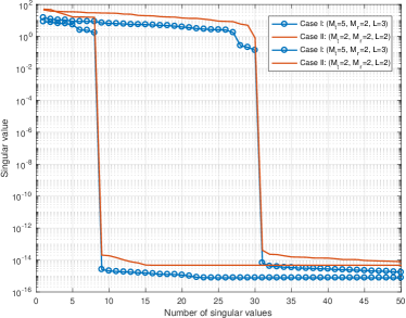
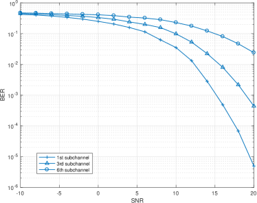
Fig. 3 illustrates the importance of the interleaver design. A random interleaver is used such that consecutive coded bits are transmitted over the same subchannel. Consequently, an error on the trellis occurs over paths that are spanned by the worst channel and the diversity order of coded multiple beamforming approaches to that of uncoded multiple beamforming with uniform power allocation. In other words, the BER performance decreases when the interleaving design criteria are not met.

Refer to caption
Figure 3: BER with respect to SNR with $N_{t}=100$, $N_{r}=50$, $M_{t}=2$, $M_{r}=2$ and $L=2$ for Ns=6subscript๐‘๐‘ 6N_{s}=6.

On the other hand, as we expect from (28), changing the number of streams Nssubscript๐‘๐‘ N_{s} should not change the diversity gain, i.e., the slope of the BER curve in high SNR. As it can be seen from Fig. 4, the slope does not change by changing the number of data streams. Hence, one can get the same diversity gain by using the maximum number of data streams available ($L_{t}$).

Refer to caption
Figure 4: BER with respect to SNR with $N_{t}=100$, $N_{r}=50$, $M_{t}=3$, $M_{r}=1$ and $L=2$ for different values of Nssubscript๐‘๐‘ N_{s}.

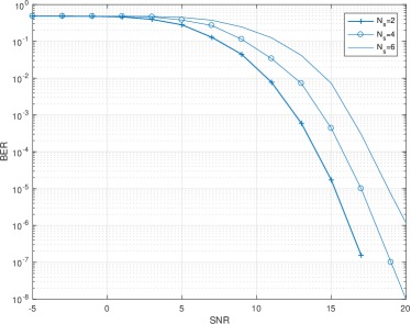
Fig. 5 illustrates the results for BICMB for both co-located and distributed mmWave massive MIMO systems. The diversity gain for the distributed system outperforms the co-located system, even though the channel in the co-located system has richer scattering (the number of propagation paths in the co-located system is twice as the distributed system). Also, as it can be seen from the figure, the curves for the distributed systems are parallel to each other, especially for the high-SNR region, which can be confirmed by (28).

Refer to caption
Figure 5: BER with respect to SNR with $N_{t}=100$, $N_{r}=50$ and Ns=3subscript๐‘๐‘ 3N_{s}=3.

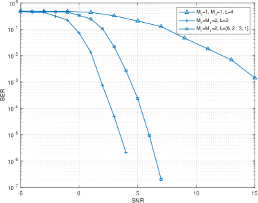
Fig. 6 illustrates the effect of the large scale fading coefficient on the diversity gain. Despite other simulations, we consider inhomogeneous large scale fading coefficients. In these simulations, information bits are mapped onto 16 quadrature amplitude modulation (QAM) symbols in each subchannel. When $M_{r}=M_{t}=2$, $L_{ij}=L=2$, $N_{t}=2N_{r}=100$ and Ns=1subscript๐‘๐‘ 1N_{s}=1 three different cases are simulated. Let $\mathcal{\mathbf{B}}=\left[\beta_{ij}\right]$ where $\beta_{ij}$ expressed in dB, as the large scale fading coefficient matrix. We used the following $\mathbf{B}$ in the simulations:

$\displaystyle\mathbf{B}_{1}=\begin{bmatrix}-20&-20\\ -20&-20\end{bmatrix},\mathbf{B}_{2}=\begin{bmatrix}-25&-25\\ -25&-25\end{bmatrix},$
$\displaystyle\mathbf{B}_{3}=\begin{bmatrix}-20&-35\\ -35&-20\end{bmatrix},\mathbf{B}_{4}=-20.$

As it can be seen from Fig. 6, when the system is homogeneous, the diversity gain remains the same. Case I and Case II, have the same slope in high SNR, which is expected. In Case III, when the system is inhomogeneous, the diversity gain decreases. By using (28), one can easily see that Case III has approximately the same diversity gain as a system with $M_{r}=M_{t}=1$ and $L=4$, i.e., $D_{G}=4$, which is depicted in Case IV.

Refer to caption
Figure 6: BER with respect to SNR with $N_{t}=100$, $N_{r}=50$ and Ns=1subscript๐‘๐‘ 1N_{s}=1.

5 Conclusion

In this paper we analyzed BICMB in mmWave massive MIMO systems. BICMB achieves full spatial diversity of $\frac{\left(\sum_{i,j}\beta_{ij}\right)^{2}}{\sum_{i,j}\beta_{ij}^{2}L_{ij}^{-1}}$ over $M_{t}$ RAU transmitters and $M_{r}$ RAU receivers. This means, by increasing the number of RAUs in the distributed system with BICMB, one can increase the diversity gain and multiplexing gain. As it can be seen from the diversity gain formula for the single-user system, the value of diversity gain is independent of the number of antennas in each RAU for both transmitter and receiver. A special case of the diversity gain where $L_{ij}=L$ and $\beta_{ij}=\beta$ would be $M_{r}M_{t}L$ which is similar to the diversity gain of a convential MIMO system.

References

  • [1] T.ย S. Rappaport, S.ย Sun, R.ย Mayzus etย al., โ€œMillimeter wave mobile communications for 5G cellular: It will work!โ€ IEEE Access, vol.ย 1, pp. 335โ€“349, May 2013.
  • [2] A.ย L. Swindlehurst, E.ย Ayanoglu, P.ย Heydari, and F.ย Capolino, โ€œMillimeter-wave massive MIMO: The next wireless revolution?โ€ IEEE Commun. Mag., vol.ย 52, no.ย 9, pp. 56โ€“62, Sep. 2014.
  • [3] W.ย Roh, J.ย Seol, J.ย Park etย al., โ€œMillimeter-wave beamforming as an enabling technology for 5G cellular communications: Theoretical feasibility and prototype results,โ€ IEEE Commun. Mag., vol.ย 52, no.ย 2, pp. 106โ€“113, Feb. 2014.
  • [4] C.ย Wang, F.ย Haider, X.ย Gao etย al., โ€œCellular architecture and key technologies for 5G wireless communication networks,โ€ IEEE Commun. Mag., vol.ย 52, no.ย 2, pp. 122โ€“130, Feb. 2014.
  • [5] E.ย Telatar, โ€œCapacity of multi-antenna Gaussian channels,โ€ Telecommun.,, vol.ย 10, no.ย 6, pp. 585โ€“595, 1999.
  • [6] Q.ย Shi, M.ย Razaviyayn, Z.-Q. Luo, and C.ย He, โ€œAn iteratively weighted MMSE approach to distributed sum-utility maximization for a MIMO interfering broadcast channel,โ€ IEEE Trans. Signal Process., vol.ย 59, no.ย 9, pp. 4331โ€“4340, Sep. 2011.
  • [7] H.ย Dahrouj and W.ย Yu, โ€œCoordinated beamforming for the multicell multi-antenna wireless system,โ€ IEEE Trans. Wireless Commun., vol.ย 9, no.ย 5, pp. 1748โ€“1759, May 2010.
  • [8] C.ย B. Peel, B.ย M. Hochwald, and A.ย L. Swindlehurst, โ€œA vector-perturbation technique for near-capacity multiantenna multiuser communication-part I: Channel inversion and regularization,โ€ IEEE Trans. Wireless Commun., vol.ย 53, no.ย 1, pp. 195โ€“202, Jan. 2005.
  • [9] C.ย H. Doan, S.ย Emami, D.ย A. Sobel etย al., โ€œDesign considerations for 60 GHz CMOS radios,โ€ IEEE Commun. Mag., vol.ย 42, no.ย 12, pp. 132โ€“140, Dec. 2004.
  • [10] F.ย Sohrabi and W.ย Yu, โ€œHybrid digital and analog beamforming design for large-scale antenna arrays,โ€ IEEE Journal of Selected Topics in Signal Processing, pp. 3476โ€“3480, 2013.
  • [11] O.ย E. Ayach, R.ย W. Heath, S.ย Abu-Surra etย al., โ€œThe capacity optimality of beam steering in large millimeter wave MIMO systems,โ€ 2012 IEEE 13th International Workshop on Signal Processing Advances in Wireless Communications (SPAWC), pp. 100โ€“104, Jun. 2012.
  • [12] O.ย E. Ayach, R.ย W. Heath, S.ย Rajagopal, and Z.ย Pi, โ€œMultimode precoding in millimeter wave MIMO transmitters with multiple antenna sub-arrays,โ€ Proc. IEEE Glob. Commun. Conf., vol.ย 42, no.ย 12, pp. 132โ€“140, Dec. 2004.
  • [13] W.ย Ni and X.ย Dong, โ€œHybrid block diagonalization for massive multiuser MIMO systems,โ€ IEEE Trans. Commun., vol.ย 64, no.ย 1, pp. 201โ€“211, Jan. 2016.
  • [14] J.ย Singh and S.ย Ramakrishna, โ€œOn the feasibility of beamforming in millimeter wave communication systems with multiple antenna arrays,โ€ Proc. IEEE GLOBECOM, pp. 3802โ€“3808, 2014.
  • [15] J.ย A. Zhang, X.ย Huang, V.ย Dyadyuk, and Y.ย J. Guo, โ€œMassive hybrid antenna array for millimeter-wave cellular communications,โ€ IEEE Wireless Commun., vol.ย 22, no.ย 1, pp. 79โ€“87, Feb. 2015.
  • [16] G.ย Caire, G.ย Taricco, and E.ย Biglieri, โ€œBit-interleaved coded modulation,โ€ IEEE Trans. Inf. Theory, vol.ย 44, no.ย 3, pp. 927โ€“946, May1998.
  • [17] E.ย Zehavi, โ€œ8-PSK trellis codes for a Rayleigh channel,โ€ IEEE Trans. Commun., vol.ย 40, no.ย 5, pp. 873โ€“884, May 1992.
  • [18] E.ย Akay, E.ย Sengul, and E.ย Ayanoglu, โ€œBit interleaved coded multiple beamforming,โ€ IEEE Trans. Commun., vol.ย 55, no.ย 9, pp. 1802โ€“1811, Sep. 2007.
  • [19] D.ย Yu, S.ย Xu, and H.ย H. Nguyen, โ€œDiversity analysis of millimeter-wave massive MIMO systems,โ€ Jan. 2018. [Online]. Available: http://arxiv.org/abs/1801.00387
  • [20] H.ย Xu, V.ย Kukshya, and T.ย Rappaport, โ€œSpatial and temporal characteristics of 60-GHz indoor channels,โ€ IEEE Journal on Selected Areas in Communications, vol.ย 20, no.ย 3, pp. 620โ€“630, 2002.
  • [21] IEEE 802.15 WPAN millimeter wave alternative PHY task group 3c. [Online] www.ieee802.org/15/pub/TG3c.html.
  • [22] R.ย V. Hogg and A.ย T. Craig, Introduction to Mathematical Statistics, 4th edition.ย ย ย New York: Macmillan, 1978.
  • [23] F.ย E. Satterthwaite, โ€œAn approximate distribution of estimates of variance components,โ€ Biometrics Bulletin, vol.ย 2, no.ย 6, pp. 110โ€“114, 1946.
  • [24] M.ย G. Bulmer, Principles of Statistics.ย ย ย Dover, 1965.