Two-Timescale Hybrid Compression and Forward for Massive MIMO Aided C-RAN

Abstract

We consider the uplink of a cloud radio access network (C-RAN), where massive MIMO remote radio heads (RRHs) serve as relays between users and a centralized baseband unit (BBU). Although employing massive MIMO at RRHs can improve the spectral efficiency, it also significantly increases the amount of data transported over the fronthaul links between RRHs and BBU, which becomes a performance bottleneck. Existing fronthaul compression methods for conventional C-RAN are not suitable for the massive MIMO regime because they require fully-digital processing and/or real-time full channel state information (CSI), incurring high implementation cost for massive MIMO RRHs. To overcome this challenge, we propose to perform a two-timescale hybrid analog-and-digital spatial filtering at each RRH to reduce the fronthaul consumption. Specifically, the analog filter is adaptive to the channel statistics to achieve massive MIMO array gain, and the digital filter is adaptive to the instantaneous effective CSI to achieve spatial multiplexing gain. Such a design can alleviate the performance bottleneck of limited fronthaul with reduced hardware cost and power consumption, and is more robust to the CSI delay. We propose an online algorithm for the two-timescale non-convex optimization of analog and digital filters, and establish its convergence to stationary solutions. Finally, simulations verify the advantages of the proposed scheme.

I Introduction

Cloud radio access network (C-RAN) [1] and massive multiple-input multiple-output (MIMO) [2] are regarded as two key technologies for future wireless systems. Both technologies can significantly improve the spectral and energy efficiency of wireless systems by employing a huge number of antennas per unit area. However, they adopt different architectures and thus have their own pros and cons.

C-RAN is essentially a large-scale distributed antenna system, where plenty of remote radio heads (RRHs) are distributed within a specific geographical area and are connected to a centralized baseband unit (BBU) pool through fronthaul links. Each RRH merely serves as a relay to forward the signals from/to the BBU via its fronthaul link, while all baseband processings are performed at the BBU. Since each user can always find some nearby RRHs with strong channel conditions, the users at different locations can enjoy a uniform quality of experience without suffering from the cell-edge effect. However, in practice, the performance of C-RAN is limited by the fronthaul capacity between each RRH’s and BBU, especially when each RRH has multiple antennas. In contrast, the massive MIMO system deploys a large number of antennas at the base station (BS) to achieve large spatial multiplexing and array gains. In this case, processing is done locally at the BS, hence the performance is no longer limited by the fronthaul capacity.

Recently, massive MIMO aided C-RAN, in which each RRH is equipped with a massive MIMO array, has been proposed to further improve the spectral and energy efficiency of wireless systems [3]. However, moving signal processing of an uplink massive MIMO system from the RRH to the cloud would require a huge amount of digital sampled data to be transported over the fronthaul link. Therefore, it is necessary to compress the uplink data at each RRH to satisfy the limited fronthaul capacity constraint. Various fully-digital fronthaul compression techniques have been proposed for the uplink of C-RAN with small-scale multi-antenna RRHs, from the more complicated quantize-and-forward (QF) schemes [4, 5] to the simpler uniform scalar quantization schemes [6] and RRH selection schemes [7]. In particular, the spatial compression and forward scheme proposed in [8] combines fully-digital linear spatial filtering and uniform scalar quantization to alleviate the performance bottleneck caused by the limited fronthaul capacity. Unfortunately, fully-digital spatial filtering requires a larger number of analog-to-digital converter (ADCs) and radio frequency (RF) chains at each massive MIMO RRH. In [9], a fully-analog linear spatial filtering is used at each RRH to achieve the fronthaul compression with reduced hardware cost and power consumption. However, fully-analog processing is known to be less efficient than hybrid analog and digital processing. Moreover, the analog filtering matrix in [9] is adapted to the instantaneous channel state information (CSI), making it difficult to be extended to wideband systems with many subcarriers, because the instantaneous CSI on different subcarriers is usually different [10].

In this paper, we propose a two-timescale hybrid (analog and digital) compression and forward (THCF) scheme for the uplink transmission of massive MIMO aided C-RAN, to alleviate the performance bottleneck of the limited fronthaul, with reduced hardware cost and power consumption. In this scheme, each RRH first performs a two-timescale hybrid analog and digital spatial filtering to reduce the dimension of its received signal. Specifically, the analog filtering matrix is adapted to the long-term channel statistics to achieve massive MIMO array gain, and the digital filtering matrix is adapted to the instantaneous effective CSI (i.e., the product of the instantaneous channel and analog filtering matrix) to achieve spatial multiplexing gain. Then, each RRH applies the uniform scalar quantization over each of these dimensions. Finally, the quantized signals at the RRHs are sent to the BBU for joint decoding. The power allocation at users, analog/digital filtering matrices and quantization bits allocation at RRHs, as well as the receive beamforming matrix at the BBU are jointly optimized to maximize a general utility function of long-term average data rates of users, including average weighted sum-rate maximization and proportional fairness (PFS) utility maximization as special cases.

Such a two-timescale hybrid design has several advantages. For example, the analog filtering matrix is robust to the CSI signaling latency. Moreover, since the channel statistics is approximately the same over different subcarriers [11], a single analog filtering matrix is sufficient to cover all subcarriers at each RRH, making it applicable to wideband systems. With the proposed THCF scheme, the massive MIMO aided C-RAN uplink system can enjoy the huge array gain provided by the massive MIMO almost for free (i.e., the complexity and power consumption are similar to the C-RAN with small-scale multi-antenna RRHs). However, there are also several technical challenges in the implementation of this architecture.

• Two-timescale Stochastic Non-convex Optimization: The joint optimization of long-term control variables (analog filtering) and short-term control variables (power allocation, digital filtering, quantization bits allocation, and receive beamforming matrix) belongs to two-timescale stochastic non-convex optimization, which is difficult to solve. Specifically, the objective function contains expectation operators and the argument of the expectation operators involves the optimal short-term control variables, which do not have closed-form expressions. In addition, the optimization of the short-term control variables at different time slots are usually coupled together for a general utility function such as PFS. Moreover, both short-term and long-term subproblems are non-convex.

• Lack of Channel Statistics: In practice, we may not even have explicit knowledge of the channel statistics. Hence, the solution should be self-learning to the unknown channel statistics.

• Convergence Analysis: It is very important to establish the convergence of the algorithm. However, this is non-trivial for a two-timescale stochastic non-convex optimization problem.

To address the above challenges, we propose an online block-coordinate stochastic successive convex approximation (BC-SSCA) algorithm with self-learning capability to solve the two-timescale stochastic non-convex optimization problem without explicit knowledge of the channel statistics. In addition, we establish convergence of the BC-SSCA algorithm to stationary solutions. Finally, simulations show that the proposed two-timescale hybrid scheme achieves better tradeoff performance than the baselines.

The rest of the paper is organized as follows. In Section II, we give the system model for two-timescale hybrid compression and forward in the uplink of massive MIMO aided C-RAN. In Section III, we formulate the two-timescale stochastic non-convex optimization problem for the joint optimization of long-term and short-term control variables. The proposed online BC-SSCA algorithm and the associated convergence proof are presented in Section IV. The simulation results are given in Section V to verify the advantages of the proposed solution, and the conclusion is given in Section VI. The key notations used in this paper are summarized in Table I.

Symbol	Parameters
$N$ ($n$)	Number of RRHs (index for RRH)
$M$	Number of antennas at each RRH
$S$	Number of RF chains at each RRH
$K$ ($k$)	Number of users (index for user)
$L$	Signal dimension after compression
$l$	Index for the entry of compressed signal
$i$	Index for time slot
$t$	Index for frame
$\bm{v}$	Digital filtering vector (short-term)
$\bm{d}$	Quantization bits allocation (short-term)
$\bm{u}$	Rx beamforming vector (short-term)
$\bm{p}$	Transmit power vector (short-term)
$\bm{\theta}$	Phase vector of analog filtering (long-term)
$\Theta$	Feasible set of $\bm{\theta}$
$\mathcal{X}$	Feasible set of the short-term variables
$\widetilde{\mathcal{X}}$	Relaxed feasible set of the short-term variables
$\Omega$	Collection of short-term variables
($r_{k}$) $r_{k}^{\circ}$	(Approximate) data rate of user $k$
($\overline{r}_{k}$) $\overline{r}_{k}^{\circ}$	(Approximate) average data rate of user $k$
$g\left(\overline{\boldsymbol{r}}\right)$	Utility function
$\hat{r}_{k}^{t}$	Recursive approximation for $\overline{r}_{k}$
$\mathbf{f}^{t}$	Recursive approximation for $\nabla_{\boldsymbol{\theta}}g\left(\overline{\boldsymbol{r}}\right)$

Table I: List of notations.

II System Model

II-A Network Architecture and Channel Model

Consider the uplink of a massive MIMO aided C-RAN, where $N$ RRHs, each equipped with a massive MIMO array of $M\gg 1$ antennas and $S<M$ Rx RF chains, are distributed within a specific geographical area to serve $K$ single-antenna users, as shown in Fig. II. Each RRH $n$ serves as a relay between the BBU and users, and is connected to the BBU via a fronthaul link of capacity $C_{n}$ bits per second (bps). The BBU is in charge of making resource allocation decisions and joint decoding of the users’ messages based on the signals from all the RRHs. We assume that the number of users $K$ is fixed and $NS\gg K$ so that there are enough spatial degrees of freedom to serve all the $K$ users. This is a typical operating regime that has been assumed in many works on massive MIMO systems [12, 10, 13]. As a motivating example, consider a system in which the users are a fixed number of pico BSs and the RRH provides backhaul links between the pico-cells and BBU.

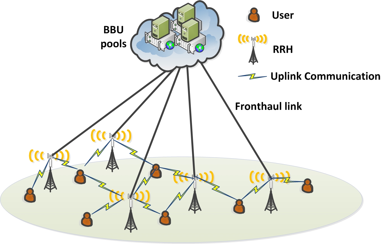
Figure 1: Uplink of a Massive MIMO aided C-RAN

For clarity, we focus on a narrowband system with flat block fading channel, but the proposed algorithm can be easily modified to cover the wideband system as well. In this case, the received signal at RRH $n$ is given by

$$\boldsymbol{y}_{n}=\sum_{k=1}^{K}\boldsymbol{h}_{n,k}\sqrt{p_{k}}s_{k}+\boldsymbol{z}_{n}=\boldsymbol{H}_{n}\boldsymbol{P}^{1/2}\boldsymbol{s}+\boldsymbol{z}_{n},$$

where $\boldsymbol{H}_{n}=\left[\boldsymbol{h}_{n,1},...,\boldsymbol{h}_{n,K}\right]\in\mathbb{C}^{M\times K}$ with $\boldsymbol{h}_{n,k}\in\mathbb{C}^{M}$ denoting the channel vector from user $k$ to RRH $n$, $\boldsymbol{s}=\left[s_{1},...,s_{K}\right]^{T}$ with $s_{k}\sim\mathcal{CN}\left(0,1\right)$ denoting the data symbol of user $k$, $\boldsymbol{P}=\text{diag}\left(p_{1},...,p_{K}\right)$ with $p_{k}$ denoting the transmit power of user $k$, and $\boldsymbol{z}_{n}\sim\mathcal{CN}\left(0,\boldsymbol{I}\right)$ is the additive white Gaussian noise vector.

II-B Two-timescale Hybrid Compression and Forward at RRHs

Each RRH $n$ applies the THCF scheme to make sure that the compressed received signal $\widetilde{\boldsymbol{y}}_{n}$ can be forward to the BBU via its fronthaul with a limited capacity of $C_{n}$ bps, as illustrated in Fig. 2. Specifically, a two-timescale hybrid filtering matrix $\boldsymbol{F}_{n}\boldsymbol{V}_{n}\in\mathbb{C}^{M\times L}$ is first applied at RRH $n$ to compress the received signal $\boldsymbol{y}_{n}$ into a low-dimensional signal $\overline{\boldsymbol{y}}_{n}=\boldsymbol{V}_{n}^{H}\boldsymbol{F}_{n}^{H}\boldsymbol{y}_{n}=\left[\overline{y}_{n,1},...,\overline{y}_{n,L}\right]^{T}\in\mathbb{C}^{L}$, where $\boldsymbol{F}_{n}\in\mathbb{C}^{M\times S}$ and $\boldsymbol{V}_{n}=\left[\boldsymbol{v}_{n,1},...,\boldsymbol{v}_{n,L}\right]\in\mathbb{C}^{S\times L}$ are the analog and digital filtering matrices, respectively, and we set $L=\mathrm{min}(K,S)$ such that there is no information loss due to digital filtering at each RRH [8]. The analog filtering matrix $\boldsymbol{F}_{n}$ is usually implemented using an RF phase shifting network [14]. Hence, $\boldsymbol{F}_{n}$ can be represented by a phase vector $\boldsymbol{\theta}_{n}\in\left[0,2\pi\right]^{MS}$, whose $\left(\left(j-1\right)M+i\right)$-th element $\theta_{n,i,j}$ is the phase of the $\left(i,j\right)$-th element of $\boldsymbol{F}_{n}$, i.e., $\left[\boldsymbol{F}_{n}\right]_{i,j}=\frac{1}{\sqrt{M}}e^{\sqrt{-1}\theta_{n,i,j}}$. In this paper, we assume that high-resolution ADCs are used at each RRH such that the quantization error due to ADCs is negligible. Then, a simple uniform scalar quantization [6] is applied to each element of $\overline{\boldsymbol{y}}_{n}$ at RRH $n$ to achieve fronthaul compression. Note that the quantization is performed at the baseband after the digital filter instead of at the ADC because we need to dynamically adjust the quantization bits according to the instantaneous channel state to improve the efficiency of fronthaul compression.

Figure 2: An illustration of the THCF scheme in Massive MIMO aided C-RAN

After the uniform scalar quantization, the compressed received signal $\widetilde{\boldsymbol{y}}_{n}=\left[\widetilde{y}_{n,1},...,\widetilde{y}_{n,L}\right]^{T}$ is modeled by

$$\widetilde{\boldsymbol{y}}_{n}=\overline{\boldsymbol{y}}_{n}+\boldsymbol{e}_{n}=\boldsymbol{V}_{n}^{H}\boldsymbol{F}_{n}^{H}\left(\boldsymbol{H}_{n}\boldsymbol{P}^{1/2}\boldsymbol{s}+\boldsymbol{z}_{n}\right)+\boldsymbol{e}_{n},$$

where $\boldsymbol{e}_{n}=\left[e_{n,1},...,e_{n,L}\right]\in\mathbb{C}^{L}$ with $e_{n,l}$ denoting the quantization error for $\overline{y}_{n,l}$. Let $d_{n,l}$ denote the number of bits that RRH $n$ uses to quantize the real or imaginary part of $\overline{y}_{n,l}$. With uniform scalar quantization, the covariance matrix of $\boldsymbol{e}_{n}$ is given by a function of $\boldsymbol{p}=\left[p_{1},...,p_{K}\right]^{T}$, $\boldsymbol{F}_{n}\boldsymbol{V}_{n}$ and $\boldsymbol{d}_{n}=\left[d_{n,1},...,d_{n,L}\right]^{T}$ as [6]

$$\boldsymbol{Q}_{n}\left(\boldsymbol{p},\boldsymbol{F}_{n}\boldsymbol{V}_{n},\boldsymbol{d}_{n}\right)=\text{diag}\left(q_{n,1},...,q_{n,L}\right),$$

where $q_{n,l}$ is the variance of the quantization error $e_{n,l}$:

$$q_{n,l}=\begin{cases}\frac{3}{4^{d_{n,l}}}(\sum_{k=1}^{K}p_{k}|\boldsymbol{h}_{n,k}^{H}\widetilde{\boldsymbol{v}}_{n,l}|^{2}+\left\|\widetilde{\boldsymbol{v}}_{n,l}\right\|^{2})&\text{if }d_{n,l}>0,\\ \infty&\text{if }d_{n,l}=0,\end{cases}$$ (1)

where $\widetilde{\boldsymbol{v}}_{n,l}=\boldsymbol{F}_{n}\boldsymbol{v}_{n,l}$. Finally, each RRH forwards the quantized bits to the BBU via the fronthaul link.

II-C Joint Rx Beamforming at the BBU

The received signal $\widetilde{\boldsymbol{y}}=\left[\widetilde{\boldsymbol{y}}_{1}^{T},...,\widetilde{\boldsymbol{y}}_{N}^{T}\right]^{T}$ at the BBU from all RRHs can be expressed as

$$\widetilde{\boldsymbol{y}}=\widetilde{\boldsymbol{V}}^{H}\boldsymbol{H}\boldsymbol{P}^{1/2}\boldsymbol{s}+\widetilde{\boldsymbol{V}}^{H}\boldsymbol{z}+\boldsymbol{e},$$

where $\widetilde{\boldsymbol{V}}=\text{diag}\left(\boldsymbol{F}_{1}\boldsymbol{V}_{1},...,\boldsymbol{F}_{N}\boldsymbol{V}_{N}\right)\in\mathbb{C}^{MN\times LN}$, $\boldsymbol{H}=\left[\boldsymbol{h}_{1},...,\boldsymbol{h}_{K}\right]\in\mathbb{C}^{MN\times K}$ with $\boldsymbol{h}_{k}=\left[\boldsymbol{h}_{1,k}^{T},...,\boldsymbol{h}_{N,k}^{T}\right]^{T}$ denoting the composite channel vector of user $k$, $\boldsymbol{z}=\left[\boldsymbol{z}_{1}^{T},...,\boldsymbol{z}_{N}^{T}\right]^{T}$, and $\boldsymbol{e}=\left[\boldsymbol{e}_{1}^{T},...,\boldsymbol{e}_{N}^{T}\right]^{T}$. A joint Rx beamforming vector $\boldsymbol{u}_{k}\in\mathbb{C}^{NL\times 1}$ is applied at the BBU to obtain the estimated data symbol for each user $k$ as

$$\hat{s}_{k} =\boldsymbol{u}_{k}^{H}\widetilde{\boldsymbol{y}}$$

$$=\boldsymbol{u}_{k}^{H}\widetilde{\boldsymbol{V}}^{H}\boldsymbol{H}\boldsymbol{P}^{1/2}\boldsymbol{s}+\boldsymbol{u}_{k}^{H}\widetilde{\boldsymbol{V}}^{H}\boldsymbol{z}+\boldsymbol{u}_{k}^{H}\boldsymbol{e},\forall k.$$

II-D Frame Structure and Achievable Data Rate

In this paper, we focus on a coherence time interval of channel statistics within which the channel statistics (distribution) are assumed to be constant. The coherence time of channel statistics is divided into $T_{f}$ frames and each frame consists of $T_{s}$ time slots, as illustrated in Fig. 3. The channel state $\boldsymbol{H}=\left\{\boldsymbol{H}_{n},\forall n\right\}$ is assumed to be constant within each time slot. In this paper, we assume that one (possibly outdated) channel sample $\boldsymbol{H}$ at each frame can be obtained by uplink channel training. Specifically, users send uplink pilot signals and then the BBU estimates the channel based on the received pilot signals collected from RRHs via the fronthaul. Several compressive sensing (CS) based channel estimation methods have been proposed for uplink channel training with a limited number of RF chains, see e.g., [15, 16]. At each time slot, the BBU needs to obtain the effective CSI $\boldsymbol{F}_{n}^{H}\boldsymbol{H}_{n}\in\mathbb{C}^{S\times K},\forall n$, which can also be obtained by uplink channel training. Since the dimension of the effective channel is equal to the number of RF chains at each RRH, a simple least-square (LS) based channel estimation method is sufficient to obtain a good estimation of the effective channel with low computation time, i.e., the delay for effective CSI can be made small relative to the channel coherence time. In our design, the BBU is not required to have explicit knowledge of the channel statistics. By observing one channel sample at each frame, the proposed algorithm can automatically learn the channel statistics (in an implicit way). Specifically, the long-term analog filtering matrices $\mathbf{F}_{n},\forall n$ are only updated once per frame based on a (possibly outdated) channel sample to achieve massive MIMO array gain with reduced implementation cost. On the other hand, the short-term control variables $\left\{\boldsymbol{p},\boldsymbol{V}_{n},\boldsymbol{d}_{n},\boldsymbol{u}_{k}\right\}$ are adaptive to the real-time effective CSI $\boldsymbol{F}_{n}^{H}\boldsymbol{H}_{n},\forall n$ to achieve the spatial multiplexing gain. For convenience, we let $\boldsymbol{v}=\textrm{Vec}\left(\left[\boldsymbol{V}_{1},...,\boldsymbol{V}_{N}\right]\right)$, $\boldsymbol{d}=\left[\boldsymbol{d}_{1}^{T},...,\boldsymbol{d}_{N}^{T}\right]^{T}$ and $\boldsymbol{u}=\left[\boldsymbol{u}_{1}^{T},...,\boldsymbol{u}_{K}^{T}\right]^{T}$.

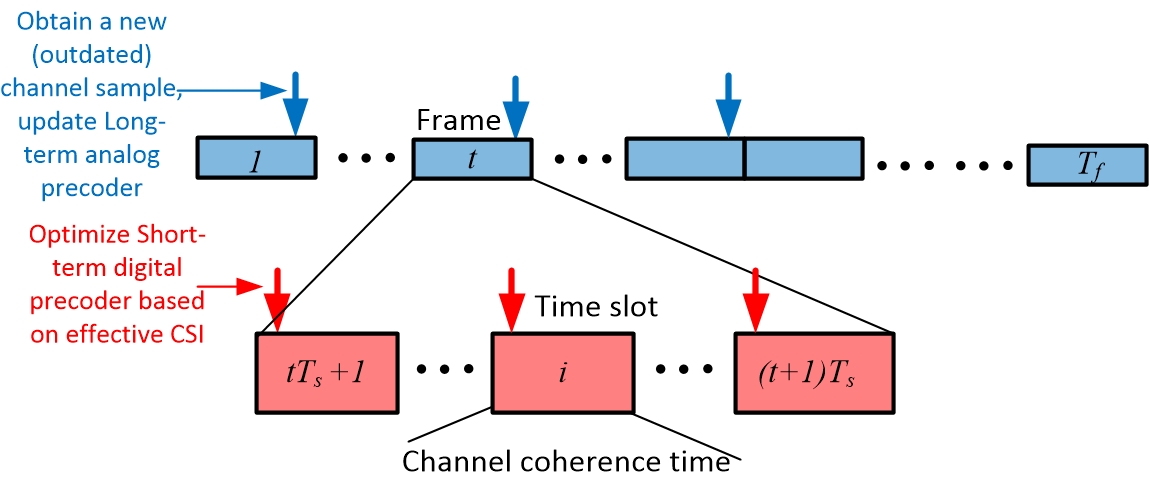
Figure 3: An illustration of two-timescale frame structure.

For given long-term control variables $\boldsymbol{\theta}=\left[\boldsymbol{\theta}_{1}^{T},...,\boldsymbol{\theta}_{n}^{T}\right]^{T}$ (phase vectors of analog filtering matrices), short-term control variables $\boldsymbol{x}\triangleq\left[\boldsymbol{p}^{T},\boldsymbol{v}^{T},\boldsymbol{d}^{T},\boldsymbol{u}^{T}\right]^{T}$ and channel realization $\boldsymbol{H}$, the achievable data rate of user $k$ is given by

$$r_{k}^{\circ}\left(\boldsymbol{\theta},\boldsymbol{x},\boldsymbol{H}\right)=\log\left(1+\text{SINR}{}_{k}\left(\boldsymbol{\theta},\boldsymbol{x};\boldsymbol{H}\right)\right),$$

where $\text{SINR}{}_{k}\left(\boldsymbol{\theta},\boldsymbol{x};\boldsymbol{H}\right)$ is the SINR of user $k$ given by

$$\text{SINR}{}_{k}\left(\boldsymbol{\theta},\boldsymbol{x};\boldsymbol{H}\right)=\;\;\;\;\;\;\;\;\;\;\;\;\;\;\;\;\;\;\;\;\;\;\;\;\;\;\;\;\;\;\;\;\;\;\;\;\;\;\;\;\;\;\;\;\;\;\;\;\;\;\;\;\;\;\;\;\;\;\;\;\;\;$$

$$\frac{p_{k}|\boldsymbol{u}_{k}^{H}\widetilde{\boldsymbol{V}}^{H}\boldsymbol{h}_{k}|^{2}}{\underset{l\neq k}{\sum}p_{l}|\boldsymbol{u}_{k}^{H}\widetilde{\boldsymbol{V}}^{H}\boldsymbol{h}_{l}|^{2}+||\boldsymbol{u}_{k}^{H}\widetilde{\boldsymbol{V}}^{H}||^{2}+\boldsymbol{u}_{k}^{H}\boldsymbol{Q}\left(\boldsymbol{\theta},\boldsymbol{p},\boldsymbol{v},\boldsymbol{d}\right)\boldsymbol{u}_{k}},$$

where

$$\boldsymbol{Q}\left(\boldsymbol{\theta},\boldsymbol{p},\boldsymbol{v},\boldsymbol{d}\right)=$$

$$\text{diag}\left(\boldsymbol{Q}_{1}\left(\boldsymbol{p},\boldsymbol{F}_{1}\boldsymbol{V}_{1},\boldsymbol{d}_{1}\right),...,\boldsymbol{Q}_{N}\left(\boldsymbol{p},\boldsymbol{F}_{N}\boldsymbol{V}_{N},\boldsymbol{d}_{N}\right)\right).$$

Note that $\boldsymbol{F}_{n}$ is a function of $\boldsymbol{\theta}_{n}$ and we will explicitly write it as $\boldsymbol{F}_{n}\left(\boldsymbol{\theta}_{n}\right)$.

Let $\boldsymbol{x}(\boldsymbol{H})$ denote the short-term control variable under channel state $\boldsymbol{H}$ and $\widetilde{\Omega}\triangleq\left\{\boldsymbol{x}(\boldsymbol{H})\in\widetilde{\mathcal{X}},\forall\boldsymbol{H}\right\}$ denote the collection of the short-term control variables for all possible channel states, with $\widetilde{\mathcal{X}}$ denoting the feasible set of the short-term control variables. To be more specific, $\widetilde{\mathcal{X}}$ is the set of all short-term control variables $\boldsymbol{x}=\left[\boldsymbol{p}^{T},\boldsymbol{v}^{T},\boldsymbol{d}^{T},\boldsymbol{u}^{T}\right]^{T}$ that satisfy the following constraints:

$$p_{k}\in\left[0,P_{k}\right], \forall k,$$ (2)

$$2B_{W}\sum_{l=1}^{L}d_{n,l}\leq C_{n}, \forall n,$$ (3)

$$d_{n,l}\geq 0\text{ is an integer,} \forall n,l,$$ (4)

where $P_{k}$ is the individual power constraint at user $k$, $B_{W}$ is the system bandwidth, and (3) is the fronthaul capacity constraint. Then the average data rate of user $k$ is

$$\overline{r}_{k}^{\circ}\left(\boldsymbol{\theta},\widetilde{\Omega}\right)=\mathbb{E}\left[r_{k}^{\circ}\left(\boldsymbol{\theta},\boldsymbol{x}(\boldsymbol{H});\boldsymbol{H}\right)\right],$$

where the expectation is taken with respect to the channel state $\boldsymbol{H}$. For convenience, define $\overline{\boldsymbol{r}}^{\circ}\left(\boldsymbol{\theta},\widetilde{\Omega}\right)\triangleq[\overline{r}_{1}^{\circ}\left(\boldsymbol{\theta},\widetilde{\Omega}\right),...,\overline{r}_{K}^{\circ}\left(\boldsymbol{\theta},\widetilde{\Omega}\right)]^{T}$ as the average data rate vector.

III Two-timescale Joint Optimization at BBU

III-A Problem Formulation

Note that $r_{k}^{\circ}\left(\boldsymbol{\theta},\boldsymbol{x},\boldsymbol{H}\right)$ is not a continuous function of $d_{n,l},\forall n,l$ because $d_{n,l}$ is an integer. To make the problem tractable, we relax the integer constraint on $d_{n,l}$ and approximate the quantization noise power $q_{n,l},\forall n,l$ with the following continuous function of a real variable $d_{n,l}\geq 0$ as

$$\hat{q}_{n,l}=\frac{3}{4^{d_{n,l}}}(\sum_{k=1}^{K}p_{k}|\boldsymbol{h}_{n,k}^{H}\widetilde{\boldsymbol{v}}_{n,l}|^{2}+\left\|\widetilde{\boldsymbol{v}}_{n,l}\right\|^{2}).$$ (5)

The same approximation has also been considered in [8]. We use $r_{k}\left(\boldsymbol{\theta},\boldsymbol{x};\boldsymbol{H}\right)$ to denote the approximate data rate of user $k$ obtained by replacing $q_{n,l}$ in (1) with $\hat{q}_{n,l}$ in (5) and the integer constraint in (4) with constraint $d_{n,l}\geq 0$. Moreover, define $\overline{\boldsymbol{r}}\left(\boldsymbol{\theta},\Omega\right)=[\overline{r}_{1}\left(\boldsymbol{\theta},\Omega\right),...,\overline{r}_{K}\left(\boldsymbol{\theta},\Omega\right)]^{T}$ as the approximate average data rate vector, where $\overline{r}_{k}\left(\boldsymbol{\theta},\Omega\right)=\mathbb{E}\left[r_{k}\left(\boldsymbol{\theta},\boldsymbol{x}(\boldsymbol{H});\boldsymbol{H}\right)\right]$ and $\Omega\triangleq\left\{\boldsymbol{x}(\boldsymbol{H})\in\mathcal{X},\forall\boldsymbol{H}\right\}$ with $\mathcal{X}$ denoting the set of all short-term control variables that satisfy constraint (2), (3) and $d_{n,l}\geq 0$. To simplify the notation, we drop the arguments in $r_{k}\left(\boldsymbol{\theta},\boldsymbol{x},\boldsymbol{H}\right)$, $\overline{\boldsymbol{r}}\left(\boldsymbol{\theta},\Omega\right)$, and write them as $r_{k}$, $\overline{\boldsymbol{r}}$, when there is no ambiguity.

With the above approximate rate, the two-timescale joint optimization of long-term and short-term control variables can be formulated as the following utility maximization problem

$$\mathcal{P}:\>\max_{\boldsymbol{\theta}\in\Theta,\Omega}\>g\left(\overline{\boldsymbol{r}}\left(\boldsymbol{\theta},\Omega\right)\right),$$ (6)

where the utility function $g\left(\overline{\boldsymbol{r}}\right)$ is continuously differentiable (and possibly non-concave) function of $\overline{\boldsymbol{r}}$, $\Theta\triangleq\left[0,2\pi\right]^{NMS}$ is the feasible set of $\boldsymbol{\theta}$. Moreover, $g\left(\overline{\boldsymbol{r}}\right)$ is non-decreasing with respect to $\overline{r}_{k},\forall k$ and its derivative $\nabla_{\overline{\boldsymbol{r}}}g\left(\overline{\boldsymbol{r}}\right)$ with respect to $\overline{\boldsymbol{r}}$ is Lipschitz continuous. This general utility function $g\left(\overline{\boldsymbol{r}}\right)$ includes many important network utilities as special cases, such as average sum rate ($g\left(\overline{\boldsymbol{r}}\right)=\sum_{k=1}^{K}\overline{r}_{k}$) and proportional fairness utility ($g\left(\overline{\boldsymbol{r}}\right)=\sum_{k=1}^{K}\log\left(\overline{r}_{k}+\varepsilon\right)$, where $\varepsilon>0$ is a small number to avoid the singularity at $\overline{r}_{k}=0$).

III-B Stationary Solution of Problem $\mathcal{P}$

Since Problem $\mathcal{P}$ is a two-timescale stochastic non-convex problem, we focus on designing an efficient algorithm to find stationary solutions of Problem $\mathcal{P}$, as defined below.

Definition 1 (Stationary solution of $\mathcal{P}$).

A solution $\left(\boldsymbol{\theta}^{*},\Omega^{*}=\left\{\boldsymbol{x}^{*}\left(\boldsymbol{H}\right)\in\mathcal{X},\forall\boldsymbol{H}\right\}\right)$ is called a stationary solution of Problem $\mathcal{P}$ if it satisfies the following conditions:

1. For every $\boldsymbol{H}$ outside a set of probability zero,

   $$\left(\boldsymbol{x}-\boldsymbol{x}^{*}(\boldsymbol{H})\right)^{T}\mathbf{J}_{\boldsymbol{x}}\left(\boldsymbol{\theta}^{*},\boldsymbol{x}^{*}(\boldsymbol{H});\boldsymbol{H}\right)\nabla_{\overline{\boldsymbol{r}}}g\left(\overline{\boldsymbol{r}}^{*}\right)\leq 0,$$ (7)

   $\forall\boldsymbol{x}\in\mathcal{X},$ where $\mathbf{J}_{\boldsymbol{x}}\left(\boldsymbol{\theta}^{*},\boldsymbol{x}^{*}(\boldsymbol{H});\boldsymbol{H}\right)$ is the Jacobian matrix of the (approximate) rate vector $\boldsymbol{r}\triangleq[r_{1},...,r_{K}]^{T}$ with respect to $\boldsymbol{x}$ at $\boldsymbol{\theta}=\boldsymbol{\theta}^{*}$ and $\boldsymbol{x}=\boldsymbol{x}^{*}(\boldsymbol{H})$, and $\nabla_{\overline{\boldsymbol{r}}}g\left(\overline{\boldsymbol{r}}^{*}\right)$ is the derivative of $g\left(\overline{\boldsymbol{r}}\right)$ at $\overline{\boldsymbol{r}}=\overline{\boldsymbol{r}}^{*}\triangleq\overline{\boldsymbol{r}}\left(\boldsymbol{\theta}^{*},\Omega^{*}\right)$.

2. $$\left(\boldsymbol{\theta}-\boldsymbol{\theta}^{*}\right)^{T}\nabla_{\boldsymbol{\theta}}g\left(\overline{\boldsymbol{r}}^{*}\right)\leq 0,\forall\boldsymbol{\theta}\in\Theta,$$ (8)

   where $\nabla_{\boldsymbol{\theta}}g\left(\overline{\boldsymbol{r}}^{*}\right)\triangleq\mathbb{E}[\mathbf{J}_{\boldsymbol{\theta}}\left(\boldsymbol{\theta}^{*},\boldsymbol{x}^{*}(\boldsymbol{H});\boldsymbol{H}\right)]\nabla_{\overline{\boldsymbol{r}}}g\left(\overline{\boldsymbol{r}}^{*}\right)$ is the partial derivative of $g\left(\overline{\boldsymbol{r}}\right)$ with respect to $\boldsymbol{\theta}$ at $\boldsymbol{\theta}=\boldsymbol{\theta}^{*}$ and $\Omega=\Omega^{*}$, $\mathbf{J}_{\boldsymbol{\theta}}\left(\boldsymbol{\theta}^{*},\boldsymbol{x}^{*}(\boldsymbol{H});\boldsymbol{H}\right)$ is the Jacobian matrix of the (approximate) rate vector $\boldsymbol{r}\left(\boldsymbol{\theta},\boldsymbol{x};\boldsymbol{H}\right)$ with respect to $\boldsymbol{\theta}$ at $\boldsymbol{\theta}=\boldsymbol{\theta}^{*}$ and $\boldsymbol{x}=\boldsymbol{x}^{*}(\boldsymbol{H})$.

In other words, a solution $\left(\boldsymbol{\theta}^{*},\Omega^{*}\right)$ is called a stationary solution of $\mathcal{P}$ if for fixed $\boldsymbol{\theta}^{*},\left\{\boldsymbol{x}^{*}(\boldsymbol{H}^{{}^{\prime}})\forall\boldsymbol{H}^{{}^{\prime}}\neq\boldsymbol{H}\right\}$, $\boldsymbol{x}^{*}(\boldsymbol{H})$ is a stationary point of $\mathcal{P}$ w.p.1., and for fixed $\Omega^{*}$, $\boldsymbol{\theta}^{*}$ is a stationary point of $\mathcal{P}$. The stationary solution is a natural extension of the stationary point for a deterministic optimization problem. The global optimal solution must be a stationary solution. However, the set of stationary solutions may also contain local optimal solutions and a certain type of saddle points. When $\mathcal{P}$ is a two-timescale stochastic convex problem, a stationary solution $\left(\boldsymbol{\theta}^{*},\Omega^{*}\right)$ is also a globally optimal solution.

Note that a stationary solution $\left(\boldsymbol{\theta}^{*},\Omega^{*}\right)$ of $\mathcal{P}$ may not satisfy all the integer constraints in (4). To obtain an integer solution for the quantization bits allocation, we use the same method as in [8] to round each $d_{n,l}^{*}$ to its nearby integer as follows.

$$\hat{d}_{n,l}\left(\alpha_{n}\right)=\begin{cases}\left\lfloor d_{n,l}^{*}\right\rfloor,&\text{if }d_{n,l}^{*}-\left\lfloor d_{n,l}^{*}\right\rfloor\leq\alpha_{n},\\ \left\lceil d_{n,l}^{*}\right\rceil,&\text{otherwise},\end{cases}\forall n,l,$$

where $0\leq\alpha_{n}\leq 1$ is chosen such that $\sum_{s=1}^{L}\hat{d}_{n,l}\left(\alpha_{n}\right)=C_{n}/2B$. Since $\sum_{l=1}^{L}\hat{d}_{n,l}\left(1\right)=\sum_{l=1}^{L}\left\lfloor d_{n,l}^{*}\right\rfloor\leq C_{n}/2B$ and $\sum_{s=1}^{L}\hat{d}_{n,l}\left(0\right)=\left\lceil d_{n,l}^{*}\right\rceil\geq C_{n}/2B$, we can always find such $\alpha_{n}$ using a bisection search over $\alpha_{n}\in\left[0,1\right]$.

IV Online Block-Coordinate Stochastic Successive Convex Approximation

There are several challenges in finding stationary solutions of Problem $\mathcal{P}$, elaborated as follows.

Challenge 1.

Complex coupling between the short-term and long-term control variables; no closed-form characterization of the average data rates $\overline{r}_{k}\left(\boldsymbol{\theta},\Omega\right),\forall k$; unknown distribution of $\boldsymbol{H}$.

To the best of our knowledge, there lacks an efficient and online algorithm with self-learning capability to handle the two-timescale stochastic non-convex optimization problem $\mathcal{P}$. In this section, we propose an online BC-SSCA algorithm to find stationary solutions of Problem $\mathcal{P}$. We shall first summarize the proposed BC-SSCA algorithm. Then we elaborate the implementation details.

IV-A Summary of the BC-SSCA Algorithm

The proposed online BC-SSCA algorithm is summarized in Algorithm 1 and its time line is illustrated in Fig. 3. In BC-SSCA, an auxiliary weight vector $\boldsymbol{\mu}=\left[\mu_{1},...,\mu_{K}\right]^{T}$ is introduced to approximate the derivative $\nabla_{\overline{\boldsymbol{r}}}g\left(\overline{\boldsymbol{r}}\right)$. At the beginning of each coherence time of channel statistics, the BBU resets the BC-SSCA algorithm with an initial analog filter phase vector $\boldsymbol{\theta}^{0}$ and a weight vector $\boldsymbol{\mu}^{0}$. Then $\boldsymbol{\theta}$ and $\boldsymbol{\mu}$ are updated once at the end of each frame, where $\boldsymbol{\theta}$ is updated by maximizing a concave surrogate function $\bar{f}^{t}\left(\boldsymbol{\theta}\right)$ of $g\left(\overline{\boldsymbol{r}}\right)$ with respect to $\boldsymbol{\theta}$. Note that we cannot obtain the optimal $\boldsymbol{\theta}$ by directly maximizing $g\left(\overline{\boldsymbol{r}}\right)$ because $g\left(\overline{\boldsymbol{r}}\right)$ is not concave and it does not have closed-form expression. Specifically, let $\boldsymbol{\theta}^{t}$ and $\boldsymbol{\mu}^{t}$ denote the analog filter phase vector and weight vector used during the $t$-th frame. The $t$-th iteration ($t$-th frame) of the BC-SSCA algorithm is described as follows.

Step 1 (Short-term control optimization at each time slot)

At time slot $i\in\left[tT_{s}+1,\left(t+1\right)T_{s}\right]$ in the $t$-th frame, the BBU first acquires the effective channel $\boldsymbol{F}_{n}^{H}\left(\boldsymbol{\theta}^{t}\right)\boldsymbol{H}_{n}\left(i\right),\forall n$, where $\boldsymbol{H}_{n}\left(i\right)$ is the channel state of RRH $n$ at time slot $i$. Then it calculates the short-term control variables $\boldsymbol{x}^{J_{t}}\left(\boldsymbol{\mu}^{t},\boldsymbol{\theta}^{t},\boldsymbol{H}(i)\right)$ from $\boldsymbol{F}_{n}^{H}\left(\boldsymbol{\theta}^{t}\right)\boldsymbol{H}_{n}(i),\forall n$ by running a short-term block-coordinate (BC) algorithm with input $J_{t}$, $\boldsymbol{\mu}^{t},\boldsymbol{\theta}^{t}$ and $\boldsymbol{H}_{n}(i)$, where $J_{t}$ determines the total number of iterations for the short-term BC algorithm at frame $t$. Note that $\boldsymbol{x}^{J_{t}}\left(\boldsymbol{\mu}^{t},\boldsymbol{\theta}^{t},\boldsymbol{H}(i)\right)$ depends on $\boldsymbol{\theta}^{t},\boldsymbol{H}(i)$ only through the effective channel $\boldsymbol{F}_{n}^{H}\left(\boldsymbol{\theta}^{t}\right)\boldsymbol{H}_{n}(i),\forall n$.

Specifically, for given input $J$, $\boldsymbol{\mu},\boldsymbol{\theta}$ and $\boldsymbol{H}$, the short-term BC algorithm runs $J$ iterations to find a stationary point (up to certain accuracy) of the following weighted sum-rate maximization problem (WSRMP):

$$\mathcal{P}_{S}\left(\boldsymbol{\mu},\boldsymbol{\theta},\boldsymbol{H}\right):\>\max_{\boldsymbol{x}=\left[\boldsymbol{p}^{T},\boldsymbol{v}^{T},\boldsymbol{d}^{T},\boldsymbol{u}^{T}\right]^{T}}\sum_{k=1}^{K}\mu_{k}r_{k}\left(\boldsymbol{\theta},\boldsymbol{x};\boldsymbol{H}\right).$$

The reason that the short-term control variables $\boldsymbol{x}^{J_{t}}\left(\boldsymbol{\mu}^{t},\boldsymbol{\theta}^{t},\boldsymbol{H}(i)\right)$ are obtained by solving the WSRMP $\mathcal{P}_{S}\left(\boldsymbol{\mu}^{t},\boldsymbol{\theta}^{t},\boldsymbol{H}(i)\right)$ is as follows. It follows from (7) that at a stationary solution $\left(\boldsymbol{\theta}^{*},\Omega^{*}=\left\{\boldsymbol{x}^{*}\left(\boldsymbol{H}\right)\in\mathcal{X},\forall\boldsymbol{H}\right\}\right)$, the short-term control variables $\boldsymbol{x}^{*}(\boldsymbol{H})$ for channel realization $\boldsymbol{H}$ must be a stationary point of $\mathcal{P}_{S}\left(\boldsymbol{\mu}^{*},\boldsymbol{\theta}^{*},\boldsymbol{H}\right)$ with a stationary weight vector $\boldsymbol{\mu}^{*}=\nabla_{\overline{\boldsymbol{r}}}g\left(\overline{\boldsymbol{r}}^{\ast}\right)$. Therefore, for fixed long-term control variable $\boldsymbol{\theta}^{*}$, once we know $\boldsymbol{\mu}^{*}$, the joint optimization of the collection of short-term control variables $\Omega$ can be decoupled into the optimization of per time slot short-term control variables by solving a WSRMP $\mathcal{P}_{S}\left(\boldsymbol{\mu}^{*},\boldsymbol{\theta}^{*},\boldsymbol{H}\left(i\right)\right)$ at each time slot $i$. However, $\boldsymbol{\mu}^{*}$ is not known a prior. Therefore, the basic idea of the proposed algorithm is to iteratively update the long-term variable $\boldsymbol{\theta}^{t}$ and the weight vector $\boldsymbol{\mu}^{t}$ such that $\boldsymbol{\theta}^{t}$ and $\boldsymbol{\mu}^{t}$ converge to a stationary solution $\boldsymbol{\theta}^{*}$ and the corresponding stationary weight vector $\boldsymbol{\mu}^{*}$, respectively. Then the short-term control variable $\boldsymbol{x}^{*}(\boldsymbol{H})$ that satisfies (7) for each channel state $\boldsymbol{H}$ can be calculated by finding a stationary point of the corresponding WSRMP $\mathcal{P}_{S}\left(\boldsymbol{\mu}^{t},\boldsymbol{\theta}^{t},\boldsymbol{H}\right)$ as $t\rightarrow\infty$.

The details of the short-term BC algorithm will be postponed to Section IV-B. Here, we only discuss the impact of $J_{t}$ on the convergence. For any finite iteration $t<\infty$, $J_{t}$ is finite, and we can let $J_{t}\rightarrow\infty$ as $t\rightarrow\infty$ to ensure the convergence to stationary solutions. A larger $J_{t}$ for fixed $t$ usually leads to a faster overall convergence speed at the cost of higher complexity.

Step 2 (Long-term control optimization at the end of frame $t$)

In Step 2a, the BBU obtains a full channel sample $\boldsymbol{H}^{t}\triangleq\boldsymbol{H}(tT_{s}+1)$ before the end of $t$-th frame. Then, in Step 2b (at the end of the $t$-th frame), the BBU updates the surrogate function $\bar{f}^{t}\left(\boldsymbol{\theta}\right)$ based on $\boldsymbol{H}^{t}$, the current iterate $\boldsymbol{\theta}^{t}$, and the short-term control variables $\boldsymbol{x}\left(i\right)\triangleq\boldsymbol{x}^{J_{t}}\left(\boldsymbol{\mu}^{t},\boldsymbol{\theta}^{t},\boldsymbol{H}(i)\right),\forall i\in\left[tT_{s}+1,\left(t+1\right)T_{s}\right]$ as

$$\bar{f}^{t}\left(\boldsymbol{\theta}\right) =g\left(\hat{\boldsymbol{r}}^{t}\right)+\left(\mathbf{f}^{t}\right)^{T}\left(\boldsymbol{\theta}-\boldsymbol{\theta}^{t}\right)-\tau\left\|\boldsymbol{\theta}-\boldsymbol{\theta}^{t}\right\|^{2},$$ (9)

where $\tau>0$ is a constant; $\hat{\boldsymbol{r}}^{t}=\left[\hat{r}_{1}^{t},...,\hat{r}_{K}^{t}\right]^{T}$ is an approximation for the average data rate vector, which is updated recursively as

$$\hat{r}_{k}^{t}=\left(1-\rho_{t}\right)\hat{r}_{k}^{t-1}+\rho_{t}\sum_{i=tT_{s}+1}^{\left(t+1\right)T_{s}}\frac{r_{k}\left(\boldsymbol{\theta}^{t},\boldsymbol{x}\left(i\right);\boldsymbol{H}\left(i\right)\right)}{T_{s}},\forall k,$$ (10)

with $\hat{r}_{k}^{-1}=0,\forall k$; $\mathbf{f}^{t}$ is an approximation of the partial derivative $\nabla_{\boldsymbol{\theta}}g\left(\overline{\boldsymbol{r}}\left(\boldsymbol{\theta},\Omega\right)\right)$ with respect to $\boldsymbol{\theta}$, which is updated recursively as

$$\mathbf{F}^{t} =\left(1-\rho_{t}\right)\mathbf{F}^{t-1}+\rho_{t}\mathbf{J}_{\boldsymbol{\theta}}\left(\boldsymbol{\theta}^{t},\boldsymbol{x}\left(tT_{s}+1\right);\boldsymbol{H}^{t}\right),$$

$$\mathbf{f}^{t} =\mathbf{F}^{t}\nabla_{\overline{\boldsymbol{r}}}g\left(\hat{\boldsymbol{r}}^{t}\right),$$ (11)

with $\mathbf{F}^{-1}=\boldsymbol{0}$, where $\rho_{t}\in\left(0,1\right]$ is a sequence to be properly chosen, $\mathbf{J}_{\boldsymbol{\theta}}\left(\boldsymbol{\theta},\boldsymbol{x};\boldsymbol{H}\right)$ is the Jacobian matrix of the rate vector $\boldsymbol{r}\left(\boldsymbol{\theta},\boldsymbol{x};\boldsymbol{H}\right)$ with respect to $\boldsymbol{\theta}$ and its expression is derived in Appendix -A, $\mathbf{F}^{t}$ is an approximation for $\mathbb{E}\left[\mathbf{J}_{\boldsymbol{\theta}}\left(\boldsymbol{\theta}^{t},\boldsymbol{x}^{J}\left(\boldsymbol{\mu}^{t},\boldsymbol{\theta}^{t},\boldsymbol{H}\right);\boldsymbol{H}\right)\right]$. It will be shown in Lemma 1 that $\hat{r}_{k}^{t}$ and $\mathbf{f}^{t}$ will converge to the true average data rate and partial derivative, respectively. Therefore, the issues of no closed-form characterization of the average data rates $\overline{r}_{k}\left(\boldsymbol{\theta},\Omega\right),\forall k$ and unknown distribution of $\boldsymbol{H}$ can be addressed by approximating the average data rate and $\nabla_{\boldsymbol{\theta}}g\left(\overline{\boldsymbol{r}}\left(\boldsymbol{\theta},\Omega\right)\right)$ in a recursive way as in (10) and (11) based on the online observations of the channel samples $\boldsymbol{H}(i)$ at each time slot $i$. Moreover, the weight vector $\boldsymbol{\mu}$ is updated as

$$\boldsymbol{\mu}^{t+1}=\left(1-\gamma_{t}\right)\boldsymbol{\mu}^{t}+\gamma_{t}\bar{\boldsymbol{\mu}}^{t}.$$ (12)

with $\bar{\boldsymbol{\mu}}^{t}\triangleq\nabla_{\overline{\boldsymbol{r}}}g\left(\hat{\boldsymbol{r}}^{t}\right)$, where $\gamma_{t}\in\left(0,1\right]$ is a sequence satisfying $\sum_{t}\gamma_{t}=\infty$, $\sum_{t}\left(\gamma_{t}\right)^{2}<\infty$.

In Step 2c, the optimal solution $\bar{\boldsymbol{\theta}}^{t}$ of the following quadratic optimization problem is solved:

$$\bar{\boldsymbol{\theta}}^{t}=\underset{\boldsymbol{\theta}\in\Theta}{\text{argmax}}\> \bar{f}^{t}\left(\boldsymbol{\theta}\right),$$ (13)

which has closed-form solution $\bar{\boldsymbol{\theta}}^{t}=\mathbb{P}_{\Theta}\left[\boldsymbol{\theta}^{t}+\frac{\mathbf{f}^{t}}{2\tau}\right]$, where $\mathbb{P}_{\Theta}\left[\cdot\right]$ denotes the projection on to the box feasible region $\Theta$. Finally, $\boldsymbol{\theta}$ is updated according to

$$\boldsymbol{\theta}^{t+1}=\left(1-\gamma_{t}\right)\boldsymbol{\theta}^{t}+\gamma_{t}\bar{\boldsymbol{\theta}}^{t}.$$ (14)

Then the above iteration is carried out until convergence.

Algorithm 1 Block-Coordinate Stochastic Successive Convex Approximation

Input: $\left\{\rho^{t}\right\}$, $\left\{\gamma^{t}\right\}$, $\left\{J_{t}\right\}$.

Initialize: $\boldsymbol{\theta}^{0}\in\Theta$; $\boldsymbol{\mu}^{0}=\left[1,...,1\right]^{T}$, $t=0$.

Step 1 (Short-term control optimization at each time slot $i\in\left[tT_{s}+1,\left(t+1\right)T_{s}\right]$):

Apply the short-term BC algorithm with input $J_{t}$, $\boldsymbol{\mu}^{t},\boldsymbol{\theta}^{t}$ and $\boldsymbol{H}_{n}(i)$, to obtain the short-term variable $\boldsymbol{x}^{J_{t}}\left(\boldsymbol{\mu}^{t},\boldsymbol{\theta}^{t},\boldsymbol{H}(i)\right)$, as elaborated in Section IV-B.

Step 2 (Long-term control optimization at the end of frame $t$):

2a: Obtain a full channel sample $\boldsymbol{H}^{t}\triangleq\boldsymbol{H}(tT_{s}+1)$.

2b: Update the surrogate function $\bar{f}^{t}\left(\boldsymbol{\theta}\right)$ according to (9) based on $\boldsymbol{H}^{t},$$\boldsymbol{\theta}^{t}$ and $\boldsymbol{x}^{J_{t}}\left(\boldsymbol{\mu}^{t},\boldsymbol{\theta}^{t},\boldsymbol{H}(i)\right),\forall i\in\left[tT_{s}+1,\left(t+1\right)T_{s}\right]$. Calculate $\bar{\boldsymbol{\mu}}^{t}=\nabla_{\overline{\boldsymbol{r}}}g\left(\hat{\boldsymbol{r}}^{t}\right)$ and update $\boldsymbol{\mu}^{t+1}$ according to (12).

2c: Solve (13) to obtain $\bar{\boldsymbol{\theta}}^{t}$. Update $\boldsymbol{\theta}^{t+1}$ according to (14).

Let $t=t+1$ and return to Step 1.

IV-B Short-term Block-Coordinate Algorithm

To apply the BC algorithm, we first transform the WSRMP $\mathcal{P}_{S}\left(\boldsymbol{\mu},\boldsymbol{\theta},\boldsymbol{H}\right)$ to the following weighted minimum mean square error (WMMSE) problem

$$\min_{\boldsymbol{\beta},\boldsymbol{v},\boldsymbol{d},\boldsymbol{u},\boldsymbol{w}} \sum_{k=1}^{K}\mu_{k}\left(w_{k}\eta_{k}-\textrm{log}w_{k}\right)$$ (15)

s.t. $$\boldsymbol{d}\geq\boldsymbol{0},\text{ (\ref{eq:Pwocons}) and (\ref{eq:frontcons})},$$

where $\boldsymbol{w}=\left[w_{1},...,w_{K}\right]$ with $w_{k}>0:\forall k$ is a weight vector for MSE, $\boldsymbol{\beta}=\left[\beta_{1},...,\beta_{k}\right]^{T}$ with $\left|\beta_{k}\right|^{2}=p_{k}$ and

$$\eta_{k}\triangleq\mathbb{E}\left[\left|s_{k}-\hat{s}_{k}\right|^{2}|\boldsymbol{H}\right]$$

$$= \left|1-\boldsymbol{u}_{k}^{H}\widetilde{\boldsymbol{V}}^{H}\boldsymbol{h}_{k}\beta_{k}\right|^{2}+\sum_{l\neq k}\left|\boldsymbol{u}_{k}^{H}\widetilde{\boldsymbol{V}}^{H}\boldsymbol{h}_{l}\beta_{l}\right|^{2}$$

$$+ \boldsymbol{u}_{k}^{H}\widetilde{\boldsymbol{V}}^{H}\widetilde{\boldsymbol{V}}\boldsymbol{u}_{k}+\boldsymbol{u}_{k}^{H}\boldsymbol{Q}\left(\boldsymbol{\theta},\boldsymbol{p},\boldsymbol{v},\boldsymbol{d}\right)\boldsymbol{u}_{k},$$

is the MSE of user $k$. Following similar proof to that of Theorem 1 in [17], it can be shown that Problem $\mathcal{P}_{S}\left(\boldsymbol{\mu},\boldsymbol{\theta},\boldsymbol{H}\right)$ is equivalent to (15). Moreover, if $\left(\boldsymbol{\beta}^{*},\boldsymbol{v}^{*},\boldsymbol{d}^{*},\boldsymbol{u}^{*},\boldsymbol{w}^{*}\right)$ is a stationary point of (15), then $\left(\boldsymbol{p}^{*},\boldsymbol{v}^{*},\boldsymbol{d}^{*},\boldsymbol{u}^{*}\right)$ is also a stationary point of $\mathcal{P}_{S}\left(\boldsymbol{\mu},\boldsymbol{\theta},\boldsymbol{H}\right)$, where $\boldsymbol{p}^{*}=\left[p_{1}^{*},...,p_{K}^{*}\right]^{T}$ with $p_{k}^{*}=\left|\beta_{k}^{*}\right|^{2}$. Therefore, we shall focus on designing a BC algorithm to find a stationary point of (15).

In the proposed BC algorithm, the short-term control variables $\boldsymbol{\beta},\boldsymbol{v},\boldsymbol{d},\boldsymbol{u},\boldsymbol{w}$ are optimized in an alternating way by solving a convex subproblem with respect to each variable. The BC algorithm is summarized in Algorithm 2. The choice of the initial point and the update equation for each variable is elaborated below.

Algorithm 2 Short-term Block-Coordinate Algorithm for $\mathcal{P}_{S}\left(\boldsymbol{\mu},\boldsymbol{\theta},\boldsymbol{H}\right)$

Input: $J$, $\boldsymbol{\mu},\boldsymbol{\theta}$ and $\boldsymbol{H}$.

Initialization: Let $j=0$, $\beta_{k}=\sqrt{P_{k}},\forall k$, $d_{n,l}=\frac{C_{n}}{2BL},\forall n,l$ and $\boldsymbol{V}_{n},\forall n$ be the first $L$ eigenvectors of $\boldsymbol{F}_{n}^{H}\boldsymbol{H}_{n}\boldsymbol{H}_{n}^{H}\boldsymbol{F}_{n}$.

Step 1 (Update $\boldsymbol{u}$, $\boldsymbol{w}$ and $\boldsymbol{\beta}$): For $k=1,...,K$, let

$$\boldsymbol{u}_{k}=\left(\sum_{l=1}^{K}\widetilde{\boldsymbol{V}}^{H}\boldsymbol{h}_{l}\left|\beta_{l}\right|^{2}\boldsymbol{h}_{l}^{H}\widetilde{\boldsymbol{V}}+\widetilde{\boldsymbol{V}}^{H}\widetilde{\boldsymbol{V}}+\boldsymbol{Q}\right)^{-1}\widetilde{\boldsymbol{V}}^{H}\boldsymbol{h}_{k}\beta_{k},$$ (16)

$$w_{k}=\left(1-\boldsymbol{u}_{k}^{H}\widetilde{\boldsymbol{V}}^{H}\boldsymbol{h}_{k}\beta_{k}\right)^{-1},$$ (17)

$$\beta_{k}=\beta_{k}^{*}\left(\lambda_{k}\right),$$ (18)

where $\beta_{k}^{*}\left(\lambda_{k}\right)$ is given in (19).

Step 2 (Update $\boldsymbol{v}$): Let $\boldsymbol{v}^{{}^{\prime}}=\boldsymbol{v}$. Update $\boldsymbol{v}$ according to (22), which depends on $\boldsymbol{v}^{{}^{\prime}}$.

Step 3 (Update $\boldsymbol{d}$): Let $d_{n,l}=d_{n,l}^{*}\left(\lambda_{n}\right),\forall n,l$, where $d_{n,l}^{*}\left(\lambda_{n}\right)$ is given in (24).

Let $j=j+1$. If $j=J$, terminate the algorithm and output $\boldsymbol{x}^{J}\left(\boldsymbol{\mu},\boldsymbol{\theta},\boldsymbol{H}\right)=\left[\boldsymbol{p}^{T},\boldsymbol{v}^{T},\boldsymbol{d}^{T},\boldsymbol{u}^{T}\right]^{T}$, where $p_{k}=\left|\beta_{k}\right|^{2},\forall k$. Otherwise, go to Step 1.

IV-B1 Choice of Initial Point

For $\boldsymbol{\beta}$, we choose the initial point to be $\beta_{k}=\sqrt{P_{k}},\forall k$, i.e., each user transmits at the maximum power. For $\boldsymbol{d}$, we choose the initial point to be $d_{n,l}=\frac{C_{n}}{2BL},\forall n,l$, i.e., equal quantization bits allocation at each RRH. For $\boldsymbol{v}$, we choose $\boldsymbol{V}_{n},\forall n$ to be the first $L$ eigenvectors of $\boldsymbol{F}_{n}^{H}\boldsymbol{H}_{n}\boldsymbol{H}_{n}^{H}\boldsymbol{F}_{n}$.

IV-B2 Optimization of $\boldsymbol{u}$, $\boldsymbol{w}$ and $\boldsymbol{\beta}$

When fixing the other short-term variables, the optimal $\boldsymbol{u}$ is given by the MMSE receiver in (16), where $\boldsymbol{Q}$ is an abbreviation for $\boldsymbol{Q}\left(\boldsymbol{\theta},\boldsymbol{p},\boldsymbol{v},\boldsymbol{d}\right)$; the optimal $w_{k}$ is given by (17); and the optimal $\boldsymbol{\beta}$ is given by $\beta_{k}=\beta_{k}^{*}\left(\lambda_{k}\right),\forall k$ with

$$\beta_{k}^{*}\left(\lambda_{k}\right) =\mu_{k}w_{k}\textrm{Re}\left[\boldsymbol{u}_{k}^{H}\widetilde{\boldsymbol{V}}^{H}\boldsymbol{h}_{k}\right]$$

$$\times\left(\sum_{l=1}^{K}2\mu_{l}w_{l}\boldsymbol{h}_{k}^{H}\widetilde{\boldsymbol{V}}\boldsymbol{u}_{l}\boldsymbol{u}_{l}^{H}\widetilde{\boldsymbol{V}}^{H}\boldsymbol{h}_{k}+\nu_{k}+2\lambda_{k}\right)^{-1},$$ (19)

where $\nu_{k}=\sum_{n,l}\frac{6}{4^{d_{n,l}}}\left|u_{k,n,l}\right|^{2}|\boldsymbol{h}_{n,k}^{H}\widetilde{\boldsymbol{v}}_{n,l}|^{2}$, $u_{k,n,l}$ is the $\left(\left(n-1\right)N+s\right)$-th element of $\boldsymbol{u}_{k}$, and $\lambda_{k}$ is chosen to be zero if $\left|\beta_{k}^{*}\left(0\right)\right|^{2}\leq P_{k}$ and chosen to satisfy $\left|\beta_{k}^{*}\left(\lambda_{k}\right)\right|^{2}=P_{k}$ otherwise.

IV-B3 Optimization of $\boldsymbol{v}$

When fixing the other short-term variables, the optimization of $\boldsymbol{v}$ is not necessarily a strictly convex problem and the optimal $\boldsymbol{v}$ may not be unique. To ensure the convergence of the short-term BC algorithm, we solve the following modified subproblem with respect to $\boldsymbol{v}$ by adding a proximal regularization term $\epsilon\left\|\boldsymbol{v}-\boldsymbol{v}^{{}^{\prime}}\right\|^{2}$:

$$\min_{\boldsymbol{v}}\sum_{k=1}^{K}\mu_{k}\left(w_{k}\eta_{k}-\textrm{log}w_{k}\right)+\epsilon\left\|\boldsymbol{v}-\boldsymbol{v}^{{}^{\prime}}\right\|^{2},$$ (20)

where $\boldsymbol{v}^{{}^{\prime}}$ is the digital filter at the beginning of the current iteration in Algorithm 2, and $\epsilon>0$ is a small positive number.

Clearly, Problem (20) is an unconstrained quadratic optimization problem. Therefore, we can obtain the optimal digital filter by checking its first-order optimality condition. After some tedious calculations, it can be shown that the first-order optimality condition can be expressed in a compact form as

$$\bm{B}v+\bm{J}+\epsilon(\boldsymbol{v}-\boldsymbol{v}^{{}^{\prime}})=0,$$ (21)

where the LHS is the gradient of the objective function in (20), $\boldsymbol{B}=\left[\boldsymbol{B}_{1,1}^{T},...,\boldsymbol{B}_{N,L}^{T}\right]^{T}$ and $\boldsymbol{B}_{n,l}=[\boldsymbol{B}_{1,1,n,l},...,\boldsymbol{B}_{N,L,n,l}]^{T}$ with

$$\boldsymbol{B}_{n^{{}^{\prime}},l^{{}^{\prime}},n,l}$$

$$= \begin{cases}\sum_{k=1}^{K}\mu_{k}w_{k}|u_{k,n,l}|^{2}(\frac{3}{4^{d_{n,l}}}+1)\boldsymbol{D}_{n},&n^{{}^{\prime}}=n,l^{{}^{\prime}}=l,\\ \sum_{k=1}^{K}\mu_{k}w_{k}u_{k,n,l}^{\ast}u_{k,n,l^{{}^{\prime}}}\boldsymbol{D}_{n},&n^{{}^{\prime}}=n,l^{{}^{\prime}}\neq l,\\ \sum_{k=1}^{K}\mu_{k}w_{k}u_{k,n,l}^{\ast}u_{k,n^{{}^{\prime}},l^{{}^{\prime}}}\boldsymbol{D}_{n,n^{{}^{\prime}}},&n^{{}^{\prime}}\neq n,\end{cases}$$

$$\boldsymbol{D}_{n} =\boldsymbol{F}_{n}^{H}\boldsymbol{F}_{n}+\sum_{k=1}^{K}\beta_{k}^{2}\boldsymbol{F}_{n}^{H}\boldsymbol{h}_{n,k}\boldsymbol{h}_{n,k}^{H}\boldsymbol{F}_{n},$$

$$\boldsymbol{D}_{n,n^{{}^{\prime}}} =\sum_{k=1}^{K}\beta_{k}^{2}\boldsymbol{F}_{n}^{H}\boldsymbol{h}_{n,k}\boldsymbol{h}_{n^{{}^{\prime}},k}\boldsymbol{F}_{n},$$

and $\boldsymbol{J}=\left[\boldsymbol{J}_{1,1},...,\boldsymbol{J}_{N,L}\right]^{T}$ with $\boldsymbol{J}_{n,l}=\sum_{k=1}^{K}\mu_{k}w_{k}\beta_{k}u_{k,n,l}^{\ast}\boldsymbol{F}_{n}^{H}\boldsymbol{h}_{n,k},\forall n,l$. From (21), the optimal digital filter for (20) is given by

$$\boldsymbol{v}=(\boldsymbol{B}+\epsilon\boldsymbol{I})^{-1}(\boldsymbol{J}+\epsilon\boldsymbol{v}^{{}^{\prime}}).$$ (22)

IV-B4 Optimization of $\boldsymbol{d}$

The subproblem with respect to $\boldsymbol{d}$ can be expressed as:

$$\min_{\boldsymbol{d}\geq\boldsymbol{0}}\sum_{k=1}^{K}\mu_{k}w_{k}\boldsymbol{u}_{k}^{H}\boldsymbol{Q}\boldsymbol{u}_{k},\text{ s.t. }\text{(\ref{eq:frontcons})},$$ (23)

Note that we have

$$\boldsymbol{u}_{k}^{H}\boldsymbol{Q}\boldsymbol{u}_{k} =\sum_{n=1}^{N}\boldsymbol{u}_{k,n}^{H}\boldsymbol{Q}_{n}\boldsymbol{u}_{k,n}=\sum_{n=1}^{N}\sum_{l=1}^{L}q_{n,l}|u_{k,n,l}|^{2}$$

$$=\sum_{n=1}^{N}\sum_{l=1}^{L}\varsigma_{k,n,l}4^{-d_{n,l}},\forall k,$$

where $\boldsymbol{Q}_{n}$ is an abbreviation for $\boldsymbol{Q}_{n}\left(\boldsymbol{p},\boldsymbol{F}_{n}\boldsymbol{V}_{n},\boldsymbol{d}_{n}\right)$, and

$$\varsigma_{k,n,l}=3|u_{k,n,l}|^{2}(\sum_{k=1}^{K}p_{k}|\boldsymbol{h}_{n,k}^{H}\widetilde{\boldsymbol{v}}_{n,l}|^{2}+\left\|\widetilde{\boldsymbol{v}}_{n,l}\right\|^{2}),\forall n,l.$$

In the following, we use the Lagrange dual method to solve subproblem (23). The Lagrange function for (23) is

$$\mathfrak{L}(\boldsymbol{d},\boldsymbol{\lambda}) =\sum_{k=1}^{K}\sum_{n=1}^{N}\sum_{l=1}^{L}\mu_{k}w_{k}\varsigma_{k,n,l}4^{-d_{n,l}},$$

$$+\sum_{n=1}^{N}\lambda_{n}(2B_{W}\sum_{l=1}^{L}d_{n,l}-C_{n}),\forall\boldsymbol{d}\geq\boldsymbol{0},$$

where $\boldsymbol{\lambda}=\left[\lambda_{1},...,\lambda_{N}\right]^{T}$ is the Lagrange multiplier vector. Since subproblem (23) is convex, the optimal quantization bits allocation can be obtained by solving the KKT conditions as

$$d_{n,l}^{*}\left(\lambda_{n}\right)=\left[\frac{\log 2B_{W}\lambda_{n}-\log(\log 4\sum_{k=1}^{K}\mu_{k}w_{k}\varsigma_{k,n,l})}{\log 4}\right]^{+},$$ (24)

$\forall n,l$, where the optimal Lagrange multiplier $\lambda_{n}\geq 0$ is chosen such that $2B_{W}\sum_{l=1}^{L}d_{n,l}^{*}\left(\lambda_{n}\right)=C_{n}$.

IV-B5 Convergence of the Short-term BC Algorithm

The short-term BC algorithm is an instance of the MM algorithm in [18]. From Theorem 4.4 in [18], we have the following result.

Theorem 1 (Convergence of Short-term BC Algorithm).

Suppose Problem (15) has a discrete set of stationary points. As $J\rightarrow\infty$, the short-term BC algorithm converges to a stationary point $\left(\boldsymbol{\beta}^{*},\boldsymbol{v}^{*},\boldsymbol{d}^{*},\boldsymbol{u}^{*},\boldsymbol{w}^{*}\right)$ of Problem (15). Moreover,

$$\left(\boldsymbol{x}-\boldsymbol{x}^{*}\right)^{T}\mathbf{J}_{\boldsymbol{x}}\left(\boldsymbol{\theta}^{*},\boldsymbol{x}^{*};\boldsymbol{H}\right)\boldsymbol{\mu}\leq 0,\forall\boldsymbol{x}\in\mathcal{\widetilde{\mathcal{X}}},$$

where $\boldsymbol{x}^{*}=\left[\boldsymbol{p}^{*T},\boldsymbol{v}^{*T},\boldsymbol{d}^{*T},\boldsymbol{u}^{*T}\right]^{T}$, and $p_{k}^{*}=\left|\beta_{k}^{*}\right|^{2},\forall k$.

In Theorem 1, we assume that Problem (15) has a discrete set of stationary points to ensure the convergence of to a single stationary point. Even if this condition is violated, the short-term BC algorithm can still converge to an invariant set of stationary points of (15) in the worst case. However, such worst-case scenario rarely occurs in practice [18, 19]. To ensure the exact convergence of the overall Algorithm 1 to stationary solutions, we need to let $J_{t}\rightarrow\infty$, as $t\rightarrow\infty$. As $t\rightarrow\infty$, the output of the short-term BC algorithm $\boldsymbol{x}^{J_{\infty}}\left(\boldsymbol{\mu},\boldsymbol{\theta},\boldsymbol{H}\right)\triangleq\lim_{t\rightarrow\infty}\boldsymbol{x}^{J_{t}}\left(\boldsymbol{\mu},\boldsymbol{\theta},\boldsymbol{H}\right)$ is well defined only when it converges to a single stationary point. Therefore, in the convergence analysis of Algorithm 1 in the next subsection, we will assume that the short-term BC algorithm converges to a single stationary point w.p.1. If we allow approximate convergence by running the short-term BC algorithm for only a finite number of iterations i.e., $\lim_{t\rightarrow\infty}J_{t}=J_{\infty}<\infty$ (which is always the case in practice), then $\boldsymbol{x}^{J_{\infty}}\left(\boldsymbol{\mu},\boldsymbol{\theta},\boldsymbol{H}\right)$ is always well defined and the assumption that Problem (15) has a discrete set of stationary points can be removed.

IV-C Convergence Analysis

In this section, we establish the local convergence of BC-SSCA to stationary solutions. Due to the complex coupling between the short-term and long-term control variables, the convergence of long-term control variable depends heavily on the properties of the short-term solution $\boldsymbol{x}^{J_{t}}\left(\boldsymbol{\mu}^{t},\boldsymbol{\theta}^{t},\boldsymbol{H}(i)\right)$ found by the short-term BC algorithm. Since there is no closed-form characterization of $\boldsymbol{x}^{J_{t}}\left(\boldsymbol{\mu}^{t},\boldsymbol{\theta}^{t},\boldsymbol{H}(i)\right)$, it is difficult to prove the convergence of BC-SSCA, which gives rise to the following challenge.

Challenge 2.

For the BC-SSCA which involves an iterative short-term BC algorithm without closed-form characterization, it is non-trivial to establish its local convergence to stationary solutions.

To address Challenge 2, we need to make the following assumptions on the parameters $\left\{\rho_{t},\gamma_{t},J_{t}\right\}$.

Assumption 1 (Assumptions on $\left\{\rho_{t},\gamma_{t},J_{t}\right\}$).

 

1. $\rho_{t}\rightarrow 0$, $\frac{1}{\rho_{t}}\leq O\left(t^{\kappa}\right)$ for some $\kappa\in\left(0,1\right)$, $\sum_{t}\left(\rho_{t}\right)^{2}<\infty$.

2. $\gamma_{t}\rightarrow 0$, $\sum_{t}\gamma_{t}=\infty$, $\sum_{t}\left(\gamma_{t}\right)^{2}<\infty$.

3. $\lim_{t\rightarrow\infty}\gamma_{t}/\rho_{t}=0$.

4. For any fixed $t>0$, $J_{t}<\infty$; and $J_{t}\rightarrow\infty$, as $t\rightarrow\infty$.

With Assumption 1, we first prove a key lemma which establishes the convergence of the recursive approximations $\hat{\boldsymbol{r}}^{t},$ $\mathbf{f}^{t}$ and the surrogate function $\bar{f}^{t}\left(\boldsymbol{\theta}\right)$.

Lemma 1 (Convergence of $\hat{\boldsymbol{r}}^{t}$, $\mathbf{f}^{t}$ and $\bar{f}^{t}\left(\boldsymbol{\theta}\right)$).

Under Assumption 1, we have

$$\lim_{t\rightarrow\infty}\left|\hat{r}_{k}^{t}-\overline{r}_{k}\left(\boldsymbol{\theta}^{t},\Omega^{J_{t}}\left(\boldsymbol{\mu}^{t},\boldsymbol{\theta}^{t}\right)\right)\right| =0,$$ (25)

$$\lim_{t\rightarrow\infty}\left\|\mathbf{f}^{t}-\nabla_{\boldsymbol{\theta}}g\left(\overline{\boldsymbol{r}}\left(\boldsymbol{\theta}^{t},\Omega^{J_{t}}\left(\boldsymbol{\mu}^{t},\boldsymbol{\theta}^{t}\right)\right)\right)\right\| =0,$$ (26)

$$\lim_{t\rightarrow\infty}\left\|\boldsymbol{\mu}^{t}-\nabla_{\overline{\boldsymbol{r}}}g\left(\overline{\boldsymbol{r}}\left(\boldsymbol{\theta}^{t},\Omega^{J_{t}}\left(\boldsymbol{\mu}^{t},\boldsymbol{\theta}^{t}\right)\right)\right)\right\| =0,$$ (27)

where $\Omega^{J}\left(\boldsymbol{\mu},\boldsymbol{\theta}\right)=\left\{\boldsymbol{x}^{J}\left(\boldsymbol{\mu},\boldsymbol{\theta},\boldsymbol{H}\right),\forall\boldsymbol{H}\right\},$ and $\boldsymbol{x}^{J}\left(\boldsymbol{\mu},\boldsymbol{\theta},\boldsymbol{H}\right)$ is the output of Algorithm 2 with input $J$, $\boldsymbol{\mu}$, $\boldsymbol{\theta}$ and $\boldsymbol{H}$. Moreover, consider a subsequence $\left\{\boldsymbol{\mu}^{t_{j}},\boldsymbol{\theta}^{t_{j}}\right\}_{j=1}^{\infty}$ converging to a limiting point $\left(\boldsymbol{\mu}^{*},\boldsymbol{\theta}^{*}\right)$, and define a function

$$\hat{f}\left(\boldsymbol{\theta}\right) \triangleq g\left(\overline{\boldsymbol{r}}\left(\boldsymbol{\theta}^{*},\Omega^{J_{\infty}}\left(\boldsymbol{\mu}^{*},\boldsymbol{\theta}^{*}\right)\right)\right)-\tau\left\|\boldsymbol{\theta}-\boldsymbol{\theta}^{*}\right\|^{2}$$

$$+\nabla_{\boldsymbol{\theta}}^{T}g\left(\overline{\boldsymbol{r}}\left(\boldsymbol{\theta}^{*},\Omega^{J_{\infty}}\left(\boldsymbol{\mu}^{*},\boldsymbol{\theta}^{*}\right)\right)\right)\left(\boldsymbol{\theta}-\boldsymbol{\theta}^{*}\right),$$

where $\Omega^{J_{\infty}}\left(\boldsymbol{\mu},\boldsymbol{\theta}\right)=\left\{\boldsymbol{x}^{J_{\infty}}\left(\boldsymbol{\mu},\boldsymbol{\theta},\boldsymbol{H}\right),\forall\boldsymbol{H}\right\},$ and $\boldsymbol{x}^{J_{\infty}}\left(\boldsymbol{\mu},\boldsymbol{\theta},\boldsymbol{H}\right)$ is the stationary point of $\mathcal{P}_{S}\left(\boldsymbol{\mu},\boldsymbol{\theta},\boldsymbol{H}\right)$ found by Algorithm 2 (i.e., run Algorithm 2 until convergence to a stationary point). Then, almost surely, we have

$$\lim_{j\rightarrow\infty}\bar{f}^{t_{j}}\left(\boldsymbol{\theta}\right) =\hat{f}\left(\boldsymbol{\theta}\right),\>\forall\boldsymbol{\theta}\in\Theta.$$ (28)

Please refer to Appendix -B for the proof. The motivation for some key assumptions and the intuition behind Lemma 1 are explained below. From the recursive update for $\hat{r}_{k}^{t}$ in (10), $\hat{r}_{k}^{t}$ is roughly obtained by averaging the instantaneous rates over a time window of size $\frac{1}{\rho_{t}}$. Since $\boldsymbol{\theta}^{t}$ is changing over time $t$, $\hat{r}_{k}^{t}$ may not converge to $\overline{r}_{k}\left(\boldsymbol{\theta}^{t},\Omega^{J_{t}}\left(\boldsymbol{\mu}^{t},\boldsymbol{\theta}^{t}\right)\right)$ in general. However, if $\lim_{t\rightarrow\infty}\gamma_{t}/\rho_{t}=0$, it follows from (14) that $\boldsymbol{\theta}^{t}$ is almost unchanged during the time window $\frac{1}{\rho_{t}}$ (i.e., $\boldsymbol{\theta}^{t-\frac{1}{\rho_{t}}}\approx\boldsymbol{\theta}^{t-\frac{1}{\rho_{t}}+1}\approx...\approx\boldsymbol{\theta}^{t-1}\approx\boldsymbol{\theta}^{t}$) for sufficiently large $t$, and thus $\hat{r}_{k}^{t}$ will converge to $\overline{r}_{k}\left(\boldsymbol{\theta}^{t},\Omega^{J_{t}}\left(\boldsymbol{\mu}^{t},\boldsymbol{\theta}^{t}\right)\right)$ as $t\rightarrow\infty$. The same assumption has also been made in single-timescale stochastic optimization (with long-term control variable only) [20] for the same reason. Another standard technical assumption $\sum_{t}\rho_{t}=\infty$ is required in single-timescale stochastic optimization. However, for the considered two-timescale stochastic optimization in which the short-term control variables $\boldsymbol{x}\left(i\right)$ are obtained by an iterative short-term BC algorithm, a slightly stronger condition $\frac{1}{\rho_{t}}\leq O\left(t^{\kappa}\right)$ with $\kappa\in\left(0,1\right)$ than $\sum_{t}\rho_{t}=\infty$ is required. With Lemma 1, the following convergence theorem can be proved.

Theorem 2 (Convergence of Algorithm 1).

Suppose Assumption 1 is satisfied. Let $\left\{\boldsymbol{\mu}^{t_{j}},\boldsymbol{\theta}^{t_{j}}\right\}_{j=1}^{\infty}$ denote any subsequence of iterates generated by Algorithm 1 that converges to a limiting point $\left(\boldsymbol{\mu}^{*},\boldsymbol{\theta}^{*}\right)$. Then we almost surely have

$$\boldsymbol{\mu}^{*}=\nabla_{\overline{\boldsymbol{r}}}g\left(\overline{\boldsymbol{r}}^{*}\right),$$

$$\left(\boldsymbol{\theta}-\boldsymbol{\theta}^{*}\right)^{T}\nabla_{\boldsymbol{\theta}}g\left(\overline{\boldsymbol{r}}\left(\boldsymbol{\theta}^{*},\Omega^{J_{\infty}}\left(\boldsymbol{\mu}^{*},\boldsymbol{\theta}^{*}\right)\right)\right)\leq 0,$$ (29)

$\forall\boldsymbol{\theta}\in\Theta$, where $\overline{\boldsymbol{r}}^{*}=\overline{\boldsymbol{r}}\left(\boldsymbol{\theta}^{*},\Omega^{J_{\infty}}\left(\boldsymbol{\mu}^{*},\boldsymbol{\theta}^{*}\right)\right)$. Moreover,

$$\lim_{j\rightarrow\infty}\left(\boldsymbol{x}-\boldsymbol{x}\left(i\right)\right)^{T}\mathbf{J}_{\boldsymbol{x}}\left(\boldsymbol{\theta}^{*},\boldsymbol{x}\left(i\right);\boldsymbol{H}(i)\right)\nabla_{\overline{\boldsymbol{r}}}g\left(\overline{\boldsymbol{r}}^{*}\right)=0,$$ (30)

where $\boldsymbol{x}\left(i\right)\triangleq\boldsymbol{x}^{J_{t_{j}}}\left(\boldsymbol{\mu}^{t_{j}},\boldsymbol{\theta}^{t_{j}},\boldsymbol{H}(i)\right),\forall i\in\left[t_{j}T_{s}+1,\left(t_{j}+1\right)T_{s}\right]$.

Please refer to Appendix -C for the proof. According to Theorem 2, as $j\rightarrow\infty$, for any $i\in\left[t_{j}T_{s}+1,\left(t_{j}+1\right)T_{s}\right]$, the short-term solution $\boldsymbol{x}\left(i\right)$ found by the short-term BC algorithm satisfies the stationary condition in (7). Moreover, the limiting point $\boldsymbol{\theta}^{*}$ generated by Algorithm 1 also satisfies the stationary condition in (8). Therefore, Algorithm 1 converges to stationary solutions of the two-timescale Problem $\mathcal{P}$.

IV-D Computational Complexity

In this subsection, we compare the computational complexity of the proposed BC-SSCA algorithm with the following baseline schemes.

• Baseline 1 - Spatial-compression-and-forward (SCF) [8]: This is the SCF scheme in [8] with the consideration of the CSI delay.

• Baseline 2 - Analog SCF (A-SCF) [9]: This is the fully-analog spatial-compression-and-forward scheme in [9].

• Baseline 3 - Slow-timescale SCF (S-SCF): This scheme is obtained by removing the short-term optimization in the proposed scheme.

We first analyze the complexity of the proposed BC-SSCA algorithm. The complexity order for other schemes can be obtained similarly.

Complexity order of the short-term BC algorithm: In each iteration of the short-term BC algorithm, we solve the subproblems for the five blocks of variables in three steps:

1) In Step 1, the calculation of $\left(\sum_{l=1}^{K}\widetilde{\boldsymbol{V}}^{H}\boldsymbol{h}_{l}\left|\beta_{l}\right|^{2}\boldsymbol{h}_{l}^{H}\widetilde{\boldsymbol{V}}+\widetilde{\boldsymbol{V}}^{H}\widetilde{\boldsymbol{V}}+\boldsymbol{Q}\right)^{-1}\in\mathbb{C}^{NL\times NL}$ and $\boldsymbol{u}_{k}$ needs $O(N^{3}L^{3})$ and $O(N^{2}L^{3})$ floating point operations (FPOs), respectively. Moreover, we only need $O(NL)$ FPOs to compute $w_{k}=\left(1-\boldsymbol{u}_{k}^{H}\widetilde{\boldsymbol{V}}^{H}\boldsymbol{h}_{k}\beta_{k}\right)^{-1}$, since $\boldsymbol{u}_{k}$ and $\widetilde{\boldsymbol{V}}^{H}\boldsymbol{h}_{k}\beta_{k}$ have been already been calculated previously. Similarly, the calculation of $\beta_{k},\forall k$ in (18) needs $O(1)$ FPOs.

2) In Step 2, the computation complexity of updating $\bm{v}$ is dominated by the inversion of $\bm{B}$ and is given by $O(N^{3}L^{3}S^{3})$.

3) In Step 3, the bisection method to find the Lagrangian parameter $\lambda_{n}$ requires $O(1)$ iterations to achieve certain accuracy and $L$ multiplications are performed in each iteration. Therefore, the computation complexity of updating $\bm{d}$ is $O(S+L).$

Based on the above analysis, the computation complexity of the short-term BC algorithm is:

$$C_{S}\triangleq O\left(N^{3}L^{3}+N^{3}L^{3}S^{3}+L\right).$$

Complexity order of the long-term control optimization: The computation complexity is dominated by the updating $\mathbf{f}$ and computing the $\mathbf{J}_{\boldsymbol{\theta}}\left(\boldsymbol{\theta},\boldsymbol{x};\boldsymbol{H}\right)$, whose complexity order is $C_{L}=O(N^{2}ML+MSNK)$.

Overall complexity order of BC-SSCA: Since each frame consists of $T_{s}$ time slots, the overall complexity order of the proposed BC-SSCA algorithm is $C_{BC-SSCA}\triangleq O\left(\text{$\frac{C_{L}}{T_{s}}$}+C_{S}\right)$.

Comparison of complexity orders: In Table II, we summarize the complexity orders of different schemes. As seen from Table II, since $M\gg S\geq L$, the proposed THCF scheme has much lower complexity than that of both the SCF scheme and the A-SCF scheme. Although the S-SCF scheme provides a lower computation complexity than that of the proposed THCF scheme, the performance is in general much worse. Consequently, our proposed THCF scheme offers a better trade-off between complexity and performance.

Schemes	Complexity order
THCF scheme	$O(\text{$\frac{N^{2}ML+MSNK}{T_{s}}$+}N^{3}L^{3}S^{3})$
SCF scheme	$O(N^{3}L^{3}M^{3})$
A-SCF scheme	$O(N^{3}L^{3}M^{3})$
S-SCF scheme	$O(\frac{N^{2}ML+MSNK}{T_{s}})$

Table II: Complexity orders for different schemes.

IV-E Implementation Consideration

At the beginning of each frame, the BBU needs to send $\boldsymbol{\theta}_{n}$ to RRH $n$. Moreover, at each time slot, the BBU needs to send $\boldsymbol{V}_{n},\boldsymbol{d}_{n}$ to RRH $n$ and $p_{k}$ to user $k$. In practice, each of these control variables $\boldsymbol{\theta}_{n},\boldsymbol{V}_{n},p_{k}$ needs to be quantized using, e.g., a codebook based method, before sending them to the RRHs or users (note that $\boldsymbol{d}_{n}$ is already an integer). The detailed codebook design for each control variable is out of the scope of this paper. In the simulations, we observe that the loss due to the quantization of $\boldsymbol{\theta}_{n}$ is already small under the simple uniform scalar quantization with only 3-bits quantization for each element. Since $\boldsymbol{\theta}_{n}$ is adaptive to the channel statistics and is only updated once per frame ($T_{f}$ time slots), the signaling overhead for communicating the quantized $\boldsymbol{\theta}_{n}$ is relatively small. On the other hand, by adapting the short-term control variables $\boldsymbol{V}_{n},\boldsymbol{d}_{n}$ and $p_{k}$ to the effective channel, these variables are updated once per time slot. Note that $\boldsymbol{V}_{n},\boldsymbol{d}_{n}$ can be conveyed to RRH $n$ via a dedicated high-speed fronthaul link and this may not cause too much overhead compared to the amount of data symbols that needs to be send to RRH $n$ (since each time slot may contain a large number of data symbols). Although $p_{k}$ needs to be send to each user $k$ via the downlink wireless channel with a lower capacity compared to the fronthaul link, it is only a scalar and thus the resulting signaling overhead is still acceptable in practice.

For users with higher mobility, the channel coherence time is smaller and the signaling overhead for sending $\boldsymbol{V}_{n},\boldsymbol{d}_{n}$ to RRH $n$ may become unacceptable. In this case, we can simply use a distributed digital filter $\boldsymbol{V}_{n}$ as in [8] such that each RRH can independently determine its digital filter $\boldsymbol{V}_{n}$ based on the covariance matrix of its received pilot signal that can be obtained locally at each RRH by sending uplink pilots from the users. Please refer to [8] for the detailed design of the distributed digital filter $\boldsymbol{V}_{n}$. In addition, we can simply use a uniform quantization (i.e., $d_{n,l}=\frac{C_{n}}{2BL},\forall n,l$) to avoid the signaling overhead of sending $\boldsymbol{d}_{n}$ to RRH $n$. Therefore, the proposed algorithm framework can be easily modified to achieve a good tradeoff between the performance and signaling overhead for practical implementations.

Remark 1.

In this paper, we focus on fast power control and thus the power allocation vector $\boldsymbol{p}$ is a short-term control variable. In practice, for high mobility user with smaller channel coherence time, we may switch to slow power control to avoid frequent fast power control signaling. The proposed algorithm can be easily modified to consider slow power control by removing the power allocation from the short-term control optimization and modifying the surrogate function for long-term control optimization to include the power allocation as a long-term variable.

V Simulation Results and Discussions

Consider a C-RAN with 4 RRHs placed in a circle cell of radius 500 m. There are 8 users randomly distributed in the cell. The channel bandwidth is 1 MHz. As in [13], we adopt a geometry-based channel model with a half-wavelength space ULA for simulations. The channel vector between RRH $n$ and user $k$ can be expressed as $\boldsymbol{h}_{n,k}=\sum_{i=1}^{N_{p}}\alpha_{n,k,i}\boldsymbol{\textrm{a}}\left(\varphi_{n,k,i}\right)$, where $\boldsymbol{\textrm{a}}\left(\varphi\right)$ is the array response vector, $\varphi_{n,k,i}$’s are Laplacian distributed with an angle spread $\sigma_{\textrm{AS}}=10$, $\alpha_{n,k,i}\sim\mathcal{CN}\left(0,\sigma_{n,k,i}^{2}\right)$, $\sigma_{n,k,i}^{2}$ are randomly generated from an exponential distribution and normalized such that $\sum_{i=1}^{N_{p}}\sigma_{n,k,i}^{2}=G_{n,k}$, $G_{n,k}$ is the average channel gain determined by the pathloss model $30.6+36.7\log 10\left(\textrm{dist}_{n,k}\right)$ [21], and $\textrm{dist}_{n,k}$ is the distance between RRH $n$ and user $k$ in meters. Unless otherwise specified, we consider $M=64$ antennas, $S=16$ RF chains and $N_{p}=6$ channel paths for each RRH. The power spectral density of the background noise is -169 dBm/Hz. The transmit power constraint for each user is $P_{k}=23$ dBm. There are $T_{s}=10$ time slots in each frame and the slot size is 1 ms. The coherence time for the channel statistics is assumed to be 10 s [22] . As in [23, 10], we assume that the CSI delay is proportional to the dimension of the channel vector that is required at the BS, i.e., if the full-CSI delay (which is defined as the delay required to obtain the full channel sample $\boldsymbol{H}_{n},\forall n$) is $\tau$ ms, then the effective-CSI delay (which is defined as the delay required to obtain the effective channel $\boldsymbol{F}_{n}^{H}\boldsymbol{H}_{n},\forall n$) is $\frac{S}{M}\tau$ ms. The carrier frequency is 2.14 GHz and the velocity of users is 3 Km/h. The CSI delay is set to be $\tau=4$ ms except for Fig. 7.

We use PFS utility as an example to illustrate the advantage of the proposed scheme. Three baseline schemes described in Section IV-D are considered for comparison. In the simulations, the performance of the ideal SCF without CSI delay is also provided as a performance upper bound.

V-A Convergence of the online BC-SSCA algorithm

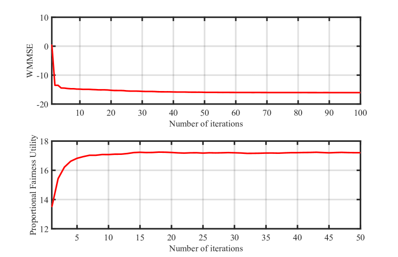
Figure 4: Convergence of the BC-SSCA algorithm.

In the upper subplot of Fig. 4, we plot the objective function of the short-term BC algorithm versus the iteration number. The short-term BC algorithm converges within a few iterations. The lower subplot illustrates the convergence behavior for the overall BC-SSCA algorithm. It can be seen that BC-SSCA quickly converges to a stationary solution.

V-B Performance versus the Fronthaul Link Capacity

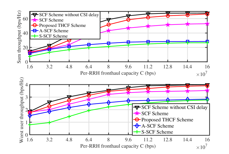
Figure 5: Rate performance versus the per-RRH fronthaul capacity $C$.

Fig. 5 shows the performance comparison of different schemes versus per-RRH fronthaul capacity $C$ varies from $C=16$ Mbps to $C=160$ Mbps. It can be observed that the best performance of both the sum throughput and worst user throughput are achieved by the SCF scheme without CSI delay, followed by the proposed THCF scheme. Furthermore, the proposed THCF scheme achieves significant gain over A-SCF and S-SCF, which demonstrates the importance of hybrid analog-and-digital processing and two-timescale joint optimization. When the fronthaul capacity increases, the performance gap between the proposed THCF scheme and the performance upper bound (SCF without CSI delay) becomes smaller. Finally, it is observed that the performance of SCF is inferior to the proposed THCF since the full-CSI delay is larger than the effective-CSI delay.

V-C Performance versus the Number of Antennas per RRH

Figure 6: Rate performance versus the per-RRH number of antennas $M$.

In Fig. 6 , we plot the rate performance versus the number of antennas $M$ per-RRH, where the per-RRH fronthaul capacity is fixed as $C=64$Mbps. We observe that the proposed THCF scheme achieves a near-optimal performance when compared to the SCF scheme without CSI delay (a performance upper bound) and outperforms the competing schemes. Moreover, as $M$ increases, the performance gap between the competing schemes becomes larger. Again, the SCF scheme without CSI delay achieves the best PFS performance, but its hardware complexity and implementation cost are much larger than the proposed THCF especially when the number of antennas $M$ per-RRH is large. Moreover, when there is CSI delay, the proposed THCF scheme will outperform the SCF scheme. In contrast, with the proposed THCF scheme, we can enjoy the huge array gain provided by the massive MIMO almost for free (i.e., the complexity and power consumption are similar to the C-RAN with small-scale multi-antenna RRHs). This indicates that the proposed THCF scheme achieves better tradeoff performance than other baselines.

V-D Performance versus the CSI Delay

Figure 7: Rate performance versus the CSI delay.

In Fig. 7, we plot the rate performance versus the CSI delay, where the per-RRH fronthaul capacity is fixed as $C=64$Mbps. We can see that as the CSI delay increases, the PFS of all schemes decreases gradually. It is observed that the PFS achieved with the proposed THCF scheme is higher than that achieved by the other schemes for moderate and large full-CSI delay. This is because the performance of the proposed THCF scheme is insensitive to the full-CSI delay. Although the performance of the S-SCF scheme is also insensitive to the full-CSI delay, its performance is still much worse than the proposed THCF scheme due to the lack of optimal power control and quantization bits allocation.

V-E Performance under Practical Implementation Consideration

Figure 8: Rate performance versus the total feedback bits per timeslot.

To illustrate the impact of quantization on the analog and digital filtering matrices in practice, the performance of all schemes are evaluated in Fig. 8 with different total numbers of quantization bits. The per-RRH fronthaul capacity is fixed as $C=64$ Mbps. For THCF, we assume that $\boldsymbol{\theta}_{n}$ is quantized using the simple uniform scalar quantization with only 3-bits quantization for each element. Moreover, the digital filter $\boldsymbol{V}_{n}$ are quantized using a random vector quantization (RVQ) codebook. For fair comparison, the total number of feedback bits per timeslot of all schemes are set to be equal. As shown in Fig. 8, the PFS utility of SCF and THCF increases with the total feedback bits per timeslot. On the other hand, the PFS utility of S-SCF and A-SCF almost remain constant when total feedback bits per timeslot ranges from 95 to 159 bits. This is because for S-SCF, a total number of 95 quantization bits corresponds to 3-bits quantization for each phase in $\boldsymbol{\theta}_{n}$, since the analog filter is updated at the slow timescale in S-SCF. In this case, the quantization loss is already small compared to the unquantized case. For A-SCF, a total number of 159 quantization bits only corresponds to less than 1-bit quantization for each phase in $\boldsymbol{\theta}_{n}$, since the analog filter is updated at the fast timescale in A-SCF. Therefore, we can only use 1-bit quantization for each phase in A-SCF for the entire range of feedback bits in the simulations. This also demonstrates that the slow-timescale/two-timescale design can significantly reduce the feedback overhead.

VI Conclusion

We propose a two-timescale hybrid compression and forward (THCF) scheme to reduce the fronthaul consumption in Massive MIMO aided C-RAN. We formulate the optimization of THCF as a general utility maximization problem, and propose a BC-SSCA algorithm to find stationary solutions of this two-stage non-convex stochastic optimization problem. At each iteration, BC-SSCA first runs an iterative BC algorithm to find a stationary point (up to a certain accuracy) of the short-term weighted sum rate maximization subproblem associated with the observed channel state. Then it updates the surrogate function for the objective of the long-term analog spatial filtering problem based on the observed channel state, the current iterate and the stationary point of the short-term subproblem. Finally, it updates the long-term analog spatial filter by solving the resulting convex approximation problem with closed-form solution. We show that the BC-SSCA algorithm converges to stationary solutions of the joint optimization problem almost surely. Finally, simulations verify that the proposed BC-SSCA algorithm achieves significant gain over existing solutions.

-A Jacobian Matrix of Instantaneous Rate

For given channel state $\boldsymbol{H},$ the Jacobian matrix of the instantaneous rate vector $r(\boldsymbol{\theta},\boldsymbol{x};\boldsymbol{H})$ with respect to $\boldsymbol{\theta}$ is

$$\mathbf{J}_{r}\left(\boldsymbol{\theta},\boldsymbol{x};\boldsymbol{H}\right)=\left[\begin{array}[]{cccc}\nabla_{\boldsymbol{\theta}}r_{1}&\nabla_{\boldsymbol{\theta}}r_{2}&\cdots&\nabla_{\boldsymbol{\theta}}r_{K}\end{array}\right],$$

where $\nabla_{\boldsymbol{\theta}}r_{k}=[\nabla_{\boldsymbol{\theta}_{1}}^{T}r_{k},...,\nabla_{\boldsymbol{\theta}_{N}}^{T}r_{k}]^{T}$. According to the matrix calculus and the chain rule, we can get

$$\nabla_{\boldsymbol{\theta}_{n}}r_{k} =\frac{\boldsymbol{a}_{n,k}}{\Gamma_{k}}-\frac{\boldsymbol{a}_{n,-k}}{\Gamma_{-k}},$$

where

$$\Gamma_{k}=\sum_{l=1}^{K}p_{l}|\boldsymbol{u}_{k}^{H}\widetilde{\boldsymbol{V}}^{H}\boldsymbol{h}_{l}|^{2}+\|\boldsymbol{u}_{k}^{H}\widetilde{\boldsymbol{V}}^{H}\|^{2}+\boldsymbol{u}_{k}^{H}\boldsymbol{Q}\left(\boldsymbol{\theta},\boldsymbol{p},\boldsymbol{v},\boldsymbol{d}\right)\boldsymbol{u}_{k},\\ \Gamma_{-k}=\sum_{l\neq k}^{K}p_{l}|\boldsymbol{u}_{k}^{H}\widetilde{\boldsymbol{V}}^{H}\boldsymbol{h}_{l}|^{2}+\|\boldsymbol{u}_{k}^{H}\widetilde{\boldsymbol{V}}^{H}\|^{2}+\boldsymbol{u}_{k}^{H}\boldsymbol{Q}\left(\boldsymbol{\theta},\boldsymbol{p},\boldsymbol{v},\boldsymbol{d}\right)\boldsymbol{u}_{k},\\ \boldsymbol{a}_{n,k}=-\mathrm{Vec}(\mathfrak{R}[\sqrt{-1}\boldsymbol{F}_{n}^{*}\circ\boldsymbol{A}_{n,k}]),\\ \boldsymbol{a}_{n,-k}=-\mathrm{Vec}(\mathfrak{R}[\sqrt{-1}\boldsymbol{F}_{n}^{*}\circ\boldsymbol{A}_{n,-k}]),\\ \boldsymbol{A}_{n,k}=\sum_{l=1}^{K}p_{l}(\boldsymbol{h}_{n,l}\boldsymbol{u}_{n,k}^{H}\boldsymbol{V}_{n}^{H})\cdot(\boldsymbol{h}_{l}^{H}\widetilde{\boldsymbol{V}}\boldsymbol{u}_{k})+\boldsymbol{F}_{n}\boldsymbol{V}_{n}\boldsymbol{u}_{n,k}\boldsymbol{u}_{n,k}^{H}\boldsymbol{V}_{n}^{H}\\ +\sum_{l=1}^{L}\frac{3u_{n,k,l}^{H}u_{n,k,l}}{4^{d_{n,l}}}(\sum_{k}p_{k}\boldsymbol{h}_{n,k}\boldsymbol{h}_{n,k}^{H}\boldsymbol{F}_{n}\boldsymbol{v}_{n.l}\boldsymbol{v}_{n,l}^{H}+\boldsymbol{F}_{n}\boldsymbol{v}_{n,l}\boldsymbol{v}_{n,l}^{H}),\\ \boldsymbol{A}_{n,-k}=\sum_{l\neq k}^{K}p_{l}(\boldsymbol{h}_{n,l}\boldsymbol{u}_{n,k}^{H}\boldsymbol{V}_{n}^{H})\cdot(\boldsymbol{h}_{l}^{H}\widetilde{\boldsymbol{V}}\boldsymbol{u}_{k})+\boldsymbol{F}_{n}\boldsymbol{V}_{n}\boldsymbol{u}_{n,k}\boldsymbol{u}_{n,k}^{H}\boldsymbol{V}_{n}^{H}\\ +\sum_{l=1}^{L}\frac{3u_{n,k,l}^{H}u_{n,k,l}}{4^{d_{n,l}}}(\sum_{k}p_{k}\boldsymbol{h}_{n,k}\boldsymbol{h}_{n,k}^{H}\boldsymbol{F}_{n}\boldsymbol{v}_{n,l}\boldsymbol{v}_{n,l}^{H}+\boldsymbol{F}_{n}\boldsymbol{v}_{n,l}\boldsymbol{v}_{n,l}^{H}).$$

-B Proof of Lemma 1

The proof relies on the following lemma which characterizes the Lipschitz continuity of $\boldsymbol{x}^{J}\left(\boldsymbol{\mu},\boldsymbol{\theta},\boldsymbol{H}\right)$ and $\overline{r}_{k}\left(\boldsymbol{\theta},\Omega^{J}\left(\boldsymbol{\mu},\boldsymbol{\theta}\right)\right),\forall k$ with respect to $\boldsymbol{\mu},\boldsymbol{\theta}$.

Lemma 2.

Let $\boldsymbol{x}^{J}\left(\boldsymbol{\mu},\boldsymbol{\theta},\boldsymbol{H}\right)$ denote the output of Algorithm 2 with input $J$, $\boldsymbol{\mu}$, $\boldsymbol{\theta}$ and $\boldsymbol{H}$. We have

$$\left\|\boldsymbol{x}^{J}\left(\boldsymbol{\mu}_{1},\boldsymbol{\theta}_{1},\boldsymbol{H}\right)-\boldsymbol{x}^{J}\left(\boldsymbol{\mu}_{2},\boldsymbol{\theta}_{2},\boldsymbol{H}\right)\right\|$$

$$\leq B_{x}^{J}\sqrt{\left\|\boldsymbol{\mu}_{1}-\boldsymbol{\mu}_{2}\right\|^{2}+\left\|\boldsymbol{\theta}_{1}-\boldsymbol{\theta}_{2}\right\|^{2}},$$ (31)

$$\left\|\overline{r}_{k}\left(\boldsymbol{\theta}_{1},\Omega^{J}\left(\boldsymbol{\mu}_{1},\boldsymbol{\theta}_{1}\right)\right)-\overline{r}_{k}\left(\boldsymbol{\theta}_{2},\Omega^{J}\left(\boldsymbol{\mu}_{2},\boldsymbol{\theta}_{2}\right)\right)\right\|$$

$$\leq B^{J}\sqrt{\left\|\boldsymbol{\mu}_{1}-\boldsymbol{\mu}_{2}\right\|^{2}+\left\|\boldsymbol{\theta}_{1}-\boldsymbol{\theta}_{2}\right\|^{2}},$$ (32)

for any $\boldsymbol{\mu}_{1}\boldsymbol{\mu}_{2}>0,\>\boldsymbol{\theta}_{1},\boldsymbol{\theta}_{2}\in\Theta$, any inner iteration number $J\geq 1$ and some constant $B_{x}>0$, $B>0$.

Proof:

In Algorithm 2, the initial point $\boldsymbol{x}^{0}\left(\boldsymbol{\mu}_{1},\boldsymbol{\theta}_{1},\boldsymbol{H}\right)-\boldsymbol{x}^{0}\left(\boldsymbol{\mu}_{2},\boldsymbol{\theta}_{2},\boldsymbol{H}\right)$ is Lipschitz continuous with respect to $\boldsymbol{\mu}$, $\boldsymbol{\theta}$. Moreover, each subproblem with respect to one short-term variable has a closed-form solution which is also Lipschitz continuous with respect to $\boldsymbol{\mu}$, $\boldsymbol{\theta}$ and the other short-term variables. Therefore, after the first iterations, we have

$$\left\|\boldsymbol{x}^{1}\left(\boldsymbol{\mu}_{1},\boldsymbol{\theta}_{1},\boldsymbol{H}\right)-\boldsymbol{x}^{1}\left(\boldsymbol{\mu}_{2},\boldsymbol{\theta}_{2},\boldsymbol{H}\right)\right\|$$

$$\leq B_{1}\sqrt{\left\|\boldsymbol{\mu}_{1}-\boldsymbol{\mu}_{2}\right\|^{2}+\left\|\boldsymbol{\theta}_{1}-\boldsymbol{\theta}_{2}\right\|^{2}},$$

for some $B_{1}>0$, and after $J$ iteration, we have

$$\left\|\boldsymbol{x}^{J}\left(\boldsymbol{\mu}_{1},\boldsymbol{\theta}_{1},\boldsymbol{H}\right)-\boldsymbol{x}^{J}\left(\boldsymbol{\mu}_{2},\boldsymbol{\theta}_{2},\boldsymbol{H}\right)\right\|$$

$$\leq B_{1}B_{2}...B_{J}\sqrt{\left\|\boldsymbol{\mu}_{1}-\boldsymbol{\mu}_{2}\right\|^{2}+\left\|\boldsymbol{\theta}_{1}-\boldsymbol{\theta}_{2}\right\|^{2}}.$$

for some $B_{j}>0,j=1,...,J$. Letting $B_{x}=\max_{j}B_{j}$, (31) is proved. Finally, (32) follows immediately from the fact that $r_{k}\left(\boldsymbol{\theta},\boldsymbol{x},\boldsymbol{H}\right)$ is Lipschitz continuous with respect to $\boldsymbol{\theta}$ and $\boldsymbol{x}$. ∎

In the rest of the proof, we will focus on proving (25). The proof for (26) and (27) is similar. We first show that for any positive integer $J>0$, we almost surely have

$$\lim_{t\rightarrow\infty}\left|\hat{r}_{k}^{t}-\overline{r}_{k}\left(\boldsymbol{\theta}^{t},\Omega^{J}\left(\boldsymbol{\mu}^{t},\boldsymbol{\theta}^{t}\right)\right)\right| \leq\overline{e}_{J},\forall k,$$ (33)

where $\overline{e}_{J}$ satisfies $\lim_{J\rightarrow\infty}\overline{e}_{J}=0$.

Step 1 of proving (33): Define a sequence

$$\tilde{r}_{k}^{t} =\left(1-\rho_{t}\right)\tilde{r}_{k}^{t-1}$$

$$+\rho_{t}\sum_{i=tT_{s}+1}^{\left(t+1\right)T_{s}}\frac{r_{k}(\boldsymbol{\theta}^{t},\boldsymbol{x}^{J}(\boldsymbol{\mu}^{t},\boldsymbol{\theta}^{t},\boldsymbol{H}(i));\boldsymbol{H}(i))}{T_{s}}.$$ (34)

Comparing (10) and (34), the update term $\sum_{i=tT_{s}+1}^{\left(t+1\right)T_{s}}\frac{r_{k}\left(\boldsymbol{\theta}^{t},\boldsymbol{x}^{J}\left(\boldsymbol{\mu}^{t},\boldsymbol{\theta}^{t},\boldsymbol{H}(i)\right);\boldsymbol{H}(i)\right)}{T_{s}}$ in (34) is only different from (10) by $e_{J,t}=\left|\frac{\sum_{i=tT_{s}+1}^{\left(t+1\right)T_{s}}(r_{k}(\boldsymbol{\theta}^{t},\boldsymbol{x}^{J}\left(\boldsymbol{\mu}^{t},\boldsymbol{\theta}^{t},\boldsymbol{H}(i)\right);\boldsymbol{H}(i))-r_{k}\left(\boldsymbol{\theta}^{t},\boldsymbol{x}(i);\boldsymbol{H}(i)\right))}{T_{s}}\right|$. Then we have

$$\lim_{t\rightarrow\infty}\left|\tilde{r}_{k}^{t}-\overline{r}_{k}\left(\boldsymbol{\theta}^{t},\Omega^{J}\left(\boldsymbol{\mu}^{t},\boldsymbol{\theta}^{t}\right)\right)\right| =0.$$ (35)

This is a consequence of [24], Lemma 1, which provides a general convergence result for any sequences of random vectors $\left\{\boldsymbol{\eta}^{t}\right\},\left\{\boldsymbol{z}^{t}\right\}$ that satisfies conditions (a) to (e) in this lemma. When applying [24], Lemma 1 to prove the convergence of $\tilde{r}_{k}^{t}$ in (35), we let $\boldsymbol{\eta}^{t}=\overline{r}_{k}\left(\boldsymbol{\theta}^{t},\Omega^{J}\left(\boldsymbol{\mu}^{t},\boldsymbol{\theta}^{t}\right)\right)$, $\boldsymbol{z}^{t}=\tilde{r}_{k}^{t}$ and $\boldsymbol{\zeta}^{t}=\sum_{i=tT_{s}+1}^{\left(t+1\right)T_{s}}\frac{r_{k}(\boldsymbol{\theta}^{t},\boldsymbol{x}^{J}(\boldsymbol{\mu}^{t},\boldsymbol{\theta}^{t},\boldsymbol{H}(i));\boldsymbol{H}(i))}{T_{s}}$. Since the instantaneous rate $r_{k}$ is bounded, we can find a convex and closed box region $\mathcal{Z}$ to contain $r_{k}$ such that condition (a) and (b) are satisfied. Since $\mathbb{E}\left[\boldsymbol{\zeta}^{t}\right]=\overline{r}_{k}\left(\boldsymbol{\theta}^{t},\Omega^{J}\left(\boldsymbol{\mu}^{t},\boldsymbol{\theta}^{t}\right)\right)$, we have $\boldsymbol{b}^{t}=\boldsymbol{0}$ in condition (c) and it follows from $\sum_{t=0}^{\infty}\left(\rho^{t}\right)^{2}<\infty$ that condition (c) is satisfied. Condition (d) follows from the assumption on $\left\{\rho^{t}\right\}$. Finally, from Lemma 2, we have

$$\lim_{t\rightarrow\infty}\frac{|\overline{r}_{k}(\boldsymbol{\theta}^{t+1},\Omega^{J}\left(\boldsymbol{\mu}^{t+1},\boldsymbol{\theta}^{t+1}\right))-\overline{r}_{k}(\boldsymbol{\theta}^{t},\Omega^{J}\left(\boldsymbol{\mu}^{t},\boldsymbol{\theta}^{t}\right))|}{\rho_{t}}$$

$$\leq \lim_{t\rightarrow\infty}O\left(\frac{\gamma^{t}B^{J}}{\rho_{t}}\right)=0,$$

where the last inequality follows from (32) and $\sqrt{\left\|\boldsymbol{\mu}^{t+1}-\boldsymbol{\mu}^{t}\right\|^{2}+\left\|\boldsymbol{\theta}^{t+1}-\boldsymbol{\theta}^{t}\right\|^{2}}=O\left(\gamma_{t}\right)$. Therefore, condition (e) in [24], Lemma 1 is also satisfied, and thus (35) follows immediately from [24], Lemma 1.

Step 2 of proving (33): By the definitions of $\tilde{r}_{k}^{t}$ and $\hat{r}_{k}^{t}$, we have

$$\left|\hat{r}_{k}^{t}-\tilde{r}_{k}^{t}\right|$$

$$\leq \sum_{t^{{}^{\prime}}=1}^{t}\left(1-\rho_{t}\right)^{t-t^{{}^{\prime}}}\rho_{t^{{}^{\prime}}}e_{J,t^{{}^{\prime}}}$$

$$= \sum_{t^{{}^{\prime}}=1}^{n_{t}}\left(1-\rho_{t}\right)^{t-t^{{}^{\prime}}}\rho_{t^{{}^{\prime}}}e_{J,t^{{}^{\prime}}}+\sum_{t^{{}^{\prime}}=n_{t}+1}^{t}\left(1-\rho_{t}\right)^{t-t^{{}^{\prime}}}\rho_{t^{{}^{\prime}}}e_{J,t^{{}^{\prime}}}$$

$$\leq \rho_{1}e_{J,t}^{a}\frac{\left(1-\rho_{t}\right)^{t-n_{t}}}{\rho_{t}}+\frac{\rho_{n_{t}+1}}{\rho_{t}}e_{J,t}^{b},$$

where $n_{t}=\left(1-\kappa-\epsilon\right)t$ with $\epsilon\in\left(0,1-\kappa\right)$, $e_{J,t}^{a}=\max_{t^{{}^{\prime}}\in\left\{1,...,n_{t}\right\}}e_{J,t^{{}^{\prime}}}$ and $e_{J,t}^{b}=\max_{t^{{}^{\prime}}\in\left\{n_{t}+1,...,t\right\}}e_{J,t^{{}^{\prime}}}$. From Assumption 1-2, we have $\lim_{t\rightarrow\infty}\rho_{1}e_{J,t}^{a}\frac{\left(1-\rho_{t}\right)^{t-n_{t}}}{\rho_{t}}=0$ and $\lim_{t\rightarrow\infty}\frac{\rho_{n_{t}+1}}{\rho_{t}}<\infty$. Moreover, from Theorem 1, we have $\lim_{J\rightarrow\infty}e_{J,t}^{b}=0,\forall t$. Then it follows from the above analysis that $\lim_{t\rightarrow\infty}\left|\hat{r}_{k}^{t}-\tilde{r}_{k}^{t}\right|\leq\overline{e}_{J}$ for some error $\overline{e}_{J}$ satisfying $\lim_{J\rightarrow\infty}\overline{e}_{J}=0$. Together with (35), it follows that (33) holds.

Then, we prove (25). From Theorem 1, we have

$$\lim_{t\rightarrow\infty}\left|\overline{r}_{k}\left(\boldsymbol{\theta}^{t},\Omega^{J_{t}}\left(\boldsymbol{\mu}^{t},\boldsymbol{\theta}^{t}\right)\right)-\overline{r}_{k}\left(\boldsymbol{\theta}^{t},\Omega^{J}\left(\boldsymbol{\mu}^{t},\boldsymbol{\theta}^{t}\right)\right)\right|=\overline{e}_{J},$$ (36)

for some error $\overline{e}_{J}$ satisfying $\lim_{J\rightarrow\infty}\overline{e}_{J}=0$. Note that (33) holds for any finite $J$. Therefore, for any $\epsilon>0$, there exists sufficiently large but finite $J$ such that $\overline{e}_{J}\leq\frac{\epsilon}{2}$. Then it follows from (33) and (36) that

$$\lim_{t\rightarrow\infty}\left|\hat{r}_{k}^{t}-\overline{r}_{k}\left(\boldsymbol{\theta}^{t},\Omega^{J_{t}}\left(\boldsymbol{\mu}^{t},\boldsymbol{\theta}^{t}\right)\right)\right| \leq\epsilon,\forall k.$$ (37)

Since (37) holds for any $\epsilon>0$, we have $\lim_{t\rightarrow\infty}\left|\hat{r}_{k}^{t}-\overline{r}_{k}\left(\boldsymbol{\theta}^{t},\Omega^{J_{t}}\left(\boldsymbol{\mu}^{t},\boldsymbol{\theta}^{t}\right)\right)\right|=0$.

Finally, (28) follows directly from (25) - (27) and the definition of $\hat{f}\left(\boldsymbol{\theta}\right)$.

-C Proof of Theorem 2

Let $\boldsymbol{\phi}=\left[\boldsymbol{\theta}^{T},\boldsymbol{\mu}^{T}\right]^{T}$ denote the composite long-term control variables. For any $\overline{t}>0$, we use $g\left(\boldsymbol{\phi}\right)$ as an abbreviation for $g\left(\overline{\boldsymbol{r}}\left(\boldsymbol{\theta},\Omega^{J_{\overline{t}}}\left(\boldsymbol{\mu},\boldsymbol{\theta}\right)\right)\right)$, $\overline{\boldsymbol{r}}^{t}$ as an abbreviation for $\overline{\boldsymbol{r}}\left(\boldsymbol{\theta}^{t},\Omega^{J_{\overline{t}}}\left(\boldsymbol{\mu}^{t},\boldsymbol{\theta}^{t}\right)\right)$, and $\overline{\boldsymbol{r}}^{t+1,t}$ as an abbreviation for $\overline{\boldsymbol{r}}\left(\boldsymbol{\theta}^{t+1},\Omega^{J_{\overline{t}}}\left(\boldsymbol{\mu}^{t},\boldsymbol{\theta}^{t}\right)\right)$, when there is no ambiguity.

1. We first prove that $\liminf_{t\rightarrow\infty}\left\|\bar{\boldsymbol{\phi}}^{t}-\boldsymbol{\phi}^{t}\right\|=0$ w.p.1.

Since $\bar{f}^{t}\left(\boldsymbol{\theta}\right)$ is uniformly strongly concave, we have

$$\nabla^{T}\bar{f}^{t}\left(\boldsymbol{\theta}^{t}\right)\boldsymbol{d}^{t}\geq\eta\left\|\boldsymbol{d}^{t}\right\|^{2}+\bar{f}^{t}\left(\bar{\boldsymbol{\theta}}^{t}\right)-\bar{f}^{t}\left(\boldsymbol{\theta}^{t}\right)\geq\eta\left\|\boldsymbol{d}^{t}\right\|^{2},$$ (38)

for some $\eta>0$, where $\boldsymbol{d}^{t}=\bar{\boldsymbol{\theta}}^{t}-\boldsymbol{\theta}^{t}$. Moreover, we have

$$g\left(\boldsymbol{\phi}^{t+1}\right) \overset{\text{a}}{\geq}g\left(\overline{\boldsymbol{r}}^{t+1,t}\right)-o\left(\gamma^{t}\right)$$

$$\overset{\text{b}}{\geq}g\left(\boldsymbol{\phi}^{t}\right)+\gamma^{t}\nabla_{\boldsymbol{\theta}}^{T}g\left(\boldsymbol{\phi}^{t}\right)\boldsymbol{d}^{t}$$

$$-L_{0}\left(\gamma^{t}\right)^{2}\left\|\boldsymbol{d}^{t}\right\|^{2}-o\left(\gamma^{t}\right)$$

$$=g\left(\boldsymbol{\phi}^{t}\right)-L_{0}\left(\gamma^{t}\right)^{2}\left\|\boldsymbol{d}^{t}\right\|^{2}-o\left(\gamma^{t}\right)$$

$$+\gamma^{t}\left(\nabla_{\boldsymbol{\theta}}^{T}g\left(\boldsymbol{\phi}^{t}\right)-\nabla^{T}\bar{f}^{t}\left(\boldsymbol{\theta}^{t}\right)+\nabla^{T}\bar{f}^{t}\left(\boldsymbol{\theta}^{t}\right)\right)\boldsymbol{d}^{t}$$

$$\geq g\left(\boldsymbol{\phi}^{t}\right)+\gamma^{t}\eta\left\|\boldsymbol{d}^{t}\right\|^{2}-o\left(\gamma^{t}\right),$$ (39)

where $o\left(\gamma^{t}\right)/\gamma^{t}\rightarrow 0$ as $t,\overline{t}\rightarrow\infty$ and $\nabla_{\boldsymbol{\theta}}g\left(\boldsymbol{\phi}^{t}\right)=\nabla_{\boldsymbol{\theta}}g\left(\overline{\boldsymbol{r}}\left(\boldsymbol{\theta}^{t},\Omega^{J_{\overline{t}}}\left(\boldsymbol{\mu}^{t},\boldsymbol{\theta}^{t}\right)\right)\right)$; (39-a) follows from the first order Taylor expansion $g\left(\overline{\boldsymbol{r}}^{t+1,t}\right)-g\left(\overline{\boldsymbol{r}}^{t+1}\right)=\nabla_{\overline{\boldsymbol{r}}}^{T}g\left(\overline{\boldsymbol{r}}^{t+1}\right)\left(\overline{\boldsymbol{r}}^{t+1,t}-\overline{\boldsymbol{r}}^{t+1}\right)+o\left(\gamma^{t}\right)$, the fact that $\left\|\boldsymbol{\mu}^{t+1}-\nabla_{\overline{\boldsymbol{r}}}g\left(\overline{\boldsymbol{r}}^{t+1}\right)\right\|=\overline{e}_{\overline{t}}$ with $\lim_{\overline{t}\rightarrow\infty}\overline{e}_{\overline{t}}=0$, and the definitions of $\overline{\boldsymbol{r}}^{t+1,t},\overline{\boldsymbol{r}}^{t+1}$; (39-b) follows from the fact that the partial derivative $\nabla_{\boldsymbol{\theta}}g\left(\boldsymbol{\phi}^{t}\right)$ is Lipschitz continuous with $L_{0}>0$ denoting the Lipschitz constant; and the last inequality follows from (38) and $\lim_{t\rightarrow\infty}\left\|\nabla_{\boldsymbol{\theta}}g\left(\boldsymbol{\phi}^{t}\right)-\nabla\bar{f}^{t}\left(\boldsymbol{\theta}^{t}\right)\right\|=\overline{e}_{\overline{t}}$. Let us show by contradiction that w.p.1. $\liminf_{t\rightarrow\infty}\left\|\bar{\boldsymbol{\phi}}^{t}-\boldsymbol{\phi}^{t}\right\|=0$. Suppose $\liminf_{t\rightarrow\infty}\left\|\bar{\boldsymbol{\phi}}^{t}-\boldsymbol{\phi}^{t}\right\|\geq\chi>0$ with a positive probability. Then we can find a realization such that $\left\|\boldsymbol{d}^{t}\right\|\geq\chi$ for all $t$. We focus next on such a realization. By choosing a sufficiently large $t_{0}$ and $\overline{t}$, there exists $\overline{\eta}>0$ such that

$$g\left(\boldsymbol{\phi}^{t+1}\right)-g\left(\boldsymbol{\phi}^{t}\right) \geq\gamma^{t}\overline{\eta}\left\|\boldsymbol{d}^{t}\right\|^{2},\forall t\geq t_{0}.$$ (40)

It follows from (40) that

$$g\left(\boldsymbol{\phi}^{t}\right)-g\left(\boldsymbol{\phi}^{t_{0}}\right)\geq\overline{\eta}\chi^{2}\sum_{j=t_{0}}^{t}\left(\gamma^{j}\right)^{2},$$

which, in view of $\sum_{j=t_{0}}^{\infty}\left(\gamma^{j}\right)^{2}=\infty$, contradicts the boundedness of $\left\{g\left(\boldsymbol{\phi}^{t}\right)\right\}$. Therefore, it must be $\liminf_{t\rightarrow\infty}\left\|\bar{\boldsymbol{\phi}}^{t}-\boldsymbol{\phi}^{t}\right\|=0$ w.p.1.

2. Then we prove that $\limsup_{t\rightarrow\infty}\left\|\bar{\boldsymbol{\phi}}^{t}-\boldsymbol{\phi}^{t}\right\|=0$ w.p.1. We first prove a useful lemma.

Lemma 3.

There exists a constant $\hat{L}>0$ such that

$$\left\|\bar{\boldsymbol{\phi}}^{t_{1}}-\bar{\boldsymbol{\phi}}^{t_{2}}\right\|\leq\hat{L}\left\|\boldsymbol{\phi}^{t_{1}}-\boldsymbol{\phi}^{t_{2}}\right\|+e\left(t_{1},t_{2}\right),$$

where $\lim_{t_{1},t_{2}\rightarrow\infty}e\left(t_{1},t_{2}\right)=0$.

Proof:

Following a similar analysis to that in Appendix -B, it can be shown that

$$\lim_{t\rightarrow\infty}\left|\bar{f}^{t}\left(\boldsymbol{\theta}\right)-\bar{g}_{\overline{t}}\left(\boldsymbol{\theta};\boldsymbol{\phi}^{t}\right)\right| =O\left(\overline{e}_{\overline{t}}\right),$$ (41)

$$\lim_{t\rightarrow\infty}\left\|\bar{\boldsymbol{\mu}}^{t}-\nabla_{\overline{\boldsymbol{r}}}g\left(\overline{\boldsymbol{r}}^{t}\right)\right\| =O\left(\overline{e}_{\overline{t}}\right),$$ (42)

where $\bar{g}_{\overline{t}}\left(\boldsymbol{\theta};\boldsymbol{\phi}^{t}\right)\triangleq g\left(\overline{\boldsymbol{r}}^{t}\right)+\nabla_{\boldsymbol{\theta}}g\left(\boldsymbol{\phi}^{t}\right)\left(\boldsymbol{\theta}-\boldsymbol{\theta}^{t}\right)-\tau\left\|\boldsymbol{\theta}-\boldsymbol{\theta}^{t}\right\|^{2}$ and $\lim_{\overline{t}\rightarrow\infty}\overline{e}_{\overline{t}}\rightarrow 0$. It can be verified that $\bar{g}_{\overline{t}}\left(\boldsymbol{\theta};\boldsymbol{\phi}^{t}\right)$ and $\nabla_{\overline{\boldsymbol{r}}}g\left(\overline{\boldsymbol{r}}^{t}\right)$ are Lipschitz continuous in $\boldsymbol{\phi}^{t}$, and thus

$$\left|\bar{g}_{\overline{t}}\left(\boldsymbol{\theta};\boldsymbol{\phi}^{t_{1}}\right)-\bar{g}_{\overline{t}}\left(\boldsymbol{\theta};\boldsymbol{\phi}^{t_{2}}\right)\right| \leq B\left\|\boldsymbol{\phi}^{t_{1}}-\boldsymbol{\phi}^{t_{2}}\right\|,$$ (43)

$$\left\|\nabla_{\overline{\boldsymbol{r}}}g\left(\overline{\boldsymbol{r}}^{t_{1}}\right)-\nabla_{\overline{\boldsymbol{r}}}g\left(\overline{\boldsymbol{r}}^{t_{2}}\right)\right\| \leq B\left\|\boldsymbol{\phi}^{t_{1}}-\boldsymbol{\phi}^{t_{2}}\right\|,\forall\boldsymbol{\theta}\in\Theta$$ (44)

for some constant $B>0$. Combining (41) to (44), we have

$$\left|\bar{f}^{t_{1}}\left(\boldsymbol{\theta}\right)-\bar{f}^{t_{2}}\left(\boldsymbol{\theta}\right)\right| \leq B\left\|\boldsymbol{\theta}^{t_{1}}-\boldsymbol{\theta}^{t_{2}}\right\|+O\left(\overline{e}_{\overline{t}}\right)+e\left(t_{1},t_{2}\right),$$ (45)

$$\left\|\bar{\boldsymbol{\mu}}^{t_{1}}-\bar{\boldsymbol{\mu}}^{t_{2}}\right\| \leq B\left\|\boldsymbol{\theta}^{t_{1}}-\boldsymbol{\theta}^{t_{2}}\right\|+O\left(\overline{e}_{\overline{t}}\right)+e\left(t_{1},t_{2}\right),$$ (46)

where $\lim_{t_{1},t_{2}\rightarrow\infty}e\left(t_{1},t_{2}\right)=0$. Since (45) holds for any $\overline{t}>0$ and $\lim_{\overline{t}\rightarrow\infty}\overline{e}_{\overline{t}}=0$, we have

$$\left|\bar{f}^{t_{1}}\left(\boldsymbol{\theta}\right)-\bar{f}^{t_{2}}\left(\boldsymbol{\theta}\right)\right|\leq B\left\|\boldsymbol{\theta}^{t_{1}}-\boldsymbol{\theta}^{t_{2}}\right\|+e\left(t_{1},t_{2}\right),\forall\boldsymbol{\theta}\in\Theta.$$ (47)

Then it follows from (47) and the Lipschitz continuity and strong convexity of $\bar{f}^{t}\left(\boldsymbol{x}\right)$ that

$$\left\|\bar{\boldsymbol{\theta}}^{t_{1}}-\bar{\boldsymbol{\theta}}^{t_{2}}\right\|\leq B_{1}B\left\|\boldsymbol{\theta}^{t_{1}}-\boldsymbol{\theta}^{t_{2}}\right\|+B_{1}e\left(t_{1},t_{2}\right),$$ (48)

for some constant $B_{1},B_{2}>0$. This is because for strictly convex problem, when the objective function (13) is changed by amount $e\left(\boldsymbol{\theta}\right)$, the optimal solution $\bar{\boldsymbol{\theta}}^{t}$ will be changed by the same order (i.e., $\pm O\left(\left|e\left(\boldsymbol{\theta}\right)\right|\right)$). Finally, Lemma 3 follows from (44) and (48). ∎

Using Lemma 3 and following the same analysis as that in [20], Proof of Theorem 1, it can be shown that $\limsup_{t\rightarrow\infty}\left\|\bar{\boldsymbol{\phi}}^{t}-\boldsymbol{\phi}^{t}\right\|=0$ w.p.1. Therefore, we have

$$\lim_{t\rightarrow\infty}\left\|\bar{\boldsymbol{\phi}}^{t}-\boldsymbol{\phi}^{t}\right\|=0,\text{ w.p.1.}$$ (49)

3. Finally, we are ready to prove the convergence theorem. By definition, we have $\lim_{j\rightarrow\infty}\bar{\boldsymbol{\mu}}^{t_{j}}=\nabla_{\overline{\boldsymbol{r}}}g\left(\overline{\boldsymbol{r}}^{*}\right)$. Then it follows from (49) that $\boldsymbol{\mu}^{*}=\lim_{j\rightarrow\infty}\boldsymbol{\mu}^{t_{j}}=\nabla_{\overline{\boldsymbol{r}}}g\left(\overline{\boldsymbol{r}}^{*}\right)$. According to (13), Lemma 1 and (49), $\boldsymbol{\theta}^{*}$ must be the optimal solution of the following convex optimization problem w.p.1.:

$$\underset{\boldsymbol{\theta}\in\Theta}{\text{max}}\> \hat{f}\left(\boldsymbol{\theta}\right).$$ (50)

From the first-order optimality condition, we have

$$\nabla^{T}\hat{f}\left(\boldsymbol{\theta}^{*}\right)\left(\boldsymbol{\theta}-\boldsymbol{\theta}^{*}\right)\leq 0,\forall\boldsymbol{\theta}\in\Theta.$$ (51)

It follows from Lemma 1 and (51) that $\boldsymbol{\theta}^{*}$ also satisfies (29). Finally, (30) follows from $\boldsymbol{\mu}^{*}=\nabla_{\overline{\boldsymbol{r}}}g\left(\overline{\boldsymbol{r}}^{*}\right)$ and Theorem 1. This completes the proof.

References

• [1] “C-RAN the road towards green RAN,” China Mobile Research Institute, Beijing, China, Report, Oct. 2011.
• [2] F. Rusek, D. Persson, B. K. Lau, E. Larsson, T. Marzetta, O. Edfors, and F. Tufvesson, “Scaling up MIMO: Opportunities and challenges with very large arrays,” IEEE Signal Process. Mag., vol. 30, no. 1, pp. 40–60, Jan. 2013.
• [3] N. Chen, B. Rong, X. Zhang, and M. Kadoch, “Scalable and flexible massive MIMO precoding for 5G H-CRAN,” IEEE Wireless Communications, vol. 24, no. 1, pp. 46–52, February 2017.
• [4] S. H. Park, O. Simeone, O. Sahin, and S. Shamai, “Robust and efficient distributed compression for cloud radio access networks,” IEEE Transactions on Vehicular Technology, vol. 62, no. 2, pp. 692–703, Feb 2013.
• [5] Y. Zhou and W. Yu, “Optimized backhaul compression for uplink cloud radio access network,” IEEE Journal on Selected Areas in Communications, vol. 32, no. 6, pp. 1295–1307, June 2014.
• [6] L. Liu, S. Bi, and R. Zhang, “Joint power control and fronthaul rate allocation for throughput maximization in OFDMA-Based cloud radio access network,” IEEE Transactions on Communications, vol. 63, no. 11, pp. 4097–4110, Nov 2015.
• [7] S. Luo, R. Zhang, and T. J. Lim, “Downlink and uplink energy minimization through user association and beamforming in C-RAN,” IEEE Transactions on Wireless Communications, vol. 14, no. 1, pp. 494–508, Jan 2015.
• [8] L. Liu and R. Zhang, “Optimized uplink transmission in multi-antenna C-RAN with spatial compression and forward,” IEEE Transactions on Signal Processing, vol. 63, no. 19, pp. 5083–5095, Oct 2015.
• [9] L. Combi and U. Spagnolini, “Hybrid beamforming in RoF fronthauling for millimeter-wave radio,” in 2017 European Conference on Networks and Communications (EuCNC), June 2017, pp. 1–5.
• [10] A. Liu and V. K. N. Lau, “Impact of CSI knowledge on the codebook-based hybrid beamforming in massive MIMO,” IEEE Transactions on Signal Processing, vol. 64, no. 24, pp. 6545–6556, Dec 2016.
• [11] A. K. Sadek, W. Su, and K. J. R. Liu, “Transmit beamforming for space-frequency coded MIMO-OFDM systems with spatial correlation feedback,” IEEE Trans. Commun., vol. 56, no. 10, pp. 1647–1655, Oct. 2008.
• [12] O. E. Ayach, S. Rajagopal, S. Abu-Surra, Z. Pi, and R. W. Heath, “Spatially sparse precoding in millimeter wave MIMO systems,” IEEE Trans. Wireless Commun., vol. 13, no. 3, pp. 1499–1513, Mar. 2014.
• [13] S. Park, J. Park, A. Yazdan, and R. W. Heath, “Exploiting spatial channel covariance for hybrid precoding in massive MIMO systems,” IEEE Trans. Signal Processing, vol. 65, no. 14, pp. 3818–3832, July 2017.
• [14] X. Zhang, A. Molisch, and S.-Y. Kung, “Variable-phase-shift-based RF-baseband codesign for MIMO antenna selection,” IEEE Trans. Signal Processing, vol. 53, no. 11, pp. 4091–4103, Nov. 2005.
• [15] A. Liu, V. Lau, M. L. Honig, and L. Lian, “Compressive RF training and channel estimation in massive MIMO with limited RF chains,” in 2017 IEEE International Conference on Communications (ICC), May 2017, pp. 1–6.
• [16] L. Lian, A. Liu, and V. K. N. Lau, “Weighted LASSO for sparse recovery with statistical prior support information,” IEEE Transactions on Signal Processing, vol. 66, no. 6, pp. 1607–1618, March 2018.
• [17] Q. Shi, M. Razaviyayn, Z.-Q. Luo, and C. He, “An iteratively weighted MMSE approach to distributed sum-utility maximization for a MIMO interfering broadcast channel,” IEEE Trans. Signal Processing, vol. 59, no. 9, pp. 4331 –4340, Sept. 2011.
• [18] M. W. Jacobson and J. A. Fessler, “An expanded theoretical treatment of iteration-dependent majorize-minimize algorithms,” IEEE Transactions on Image Processing, vol. 16, no. 10, pp. 2411–2422, Oct 2007.
• [19] J. D. Lee, M. Simchowitz, M. I. Jordan, and B. Recht, “Gradient descent only converges to minimizers,” in In Conference on Learning Theory, June 2016, pp. 1246–1257.
• [20] Y. Yang, G. Scutari, D. P. Palomar, and M. Pesavento, “A parallel decomposition method for nonconvex stochastic multi-agent optimization problems,” IEEE Trans. Signal Processing, vol. 64, no. 11, pp. 2949–2964, June 2016.
• [21] Technical Specification Group Radio Access Network; Further Advancements for E-UTRA Physical Layer Aspects, 3GPP TR 36.814. [Online]. Available: http://www.3gpp.org
• [22] I. Viering, H. Hofstetter, and W. Utschick, “Spatial long-term variation in urban, rural and indoor environments,” in Proceedings of the 5th COST, vol. 273, 2002.
• [23] A. Liu and V. K. N. Lau, “Phase only RF precoding for massive MIMO systems with limited RF chains,” IEEE Trans. Signal Processing, vol. 62, no. 17, pp. 4505–4515, Sept. 2014.
• [24] A. Ruszczynski, “Feasible direction methods for stochastic programming problems,” Math. Programm., vol. 19, no. 1, pp. 220–229, Dec. 1980.