Dynamical structure of the pulsating atmosphere of RR Lyrae 

Abstract

Context. RRab stars are large amplitude pulsating stars in which the pulsation wave is a progressive wave. Consequently, strong shocks, stratification effects, and phase lag may exist between the variations associated with line profiles formed in different parts of the atmosphere, including the shock wake. The pulsation is associated with a large extension of the expanding atmosphere, and strong infalling motions are expected.

Aims. The objective of this study is to provide a general overview of the dynamical structure of the atmosphere occurring over a typical pulsation cycle.

Methods. We report new high-resolution observations with suitable time resolution of H$\alpha$ and sodium lines in the brightest RR Lyrae star of the sky: RR Lyr (HD 182989). A detailed analysis of line profile variations over the whole pulsation cycle is performed to understand the dynamical structure of the atmosphere.

Results. The main shock wave appears when it exits from the photosphere at $\varphi\simeq 0.89$, i.e., when the main H$\alpha$ emission is observed. Whereas the acceleration phase of the shock is not observed, a significant deceleration of the shock front velocity is clearly present. The radiative stage of the shock wave is short: $4\%$ of the pulsation period ($0.892<\varphi<0.929$). A Mach number $M>10$ is required to get such a radiative shock. The sodium layer reaches its maximum expansion well before that of H$\alpha$ ($\Delta\varphi=0.135$). Thus, a rarefaction wave is induced between the H$\alpha$ and sodium layers. A strong atmospheric compression occurring around $\varphi=0.36$, which produces the third H$\alpha$ emission, takes place in the highest part of the atmosphere. The region located lower in the atmosphere where the sodium line is formed is not involved. The amplification of gas turbulence seems mainly due to strong shock waves propagating in the atmosphere rather than to the global compression of the atmosphere caused by the pulsation. It has not yet been clearly established whether the microturbulence velocity increases or decreases with height in the atmosphere. Furthermore, it seems very probable that an interstellar component is visible within the sodium profile.

1 Introduction

The kinematics and dynamics of the outer layers of pulsating stars, a fortiori those undergoing Blazhko effect (Blazhko, 1907), is usually not known in detail. Among variable stars, RR Lyr is the brightest RR Lyrae star of the sky with $7\la\textrm{V}\la 8$. During its pulsation cycle, its photospheric radius relative variation $\Delta R_{\star}/R_{\star}=17\%$ (Fokin & Gillet, 1997), while is spectral type evolves from A7III to F8III (Gillet & Crowe, 1988). RR Lyr variability was discovered by the Scottish astronomer Williamina Fleming at Harvard in 1901 (Pickering et al., 1901). The pulsation cycle occurs on approximately 0.5668 d or, equivalently, 13.6 h. Furthermore, the light curve also presents light modulations with a variable period around 39 d. These amplitude and phase modulations are known as the Blazhko effect. Its physical origin has remained a mystery up to the present day, but recently several interesting ideas were proposed to explain the Blazhko phenomenon (Smolec, 2016; Kovács, 2016). All these phenomena are the rendering of atmospheric movements that are not simple outward and inward movements that may show light curves (see RR41 run of Fokin & Gillet 1997).

In order to study the atmospheric dynamics, the whole pulsation cycle has to be recorded in detail. The first detailed spectroscopic study of RR Lyr was done by Preston et al. (1965) during a Blazhko cycle, but this investigation was limited to the pulsation phases of rising light within the 13.6 h cycle. Chadid & Gillet (1996) carried on spectroscopic observation and showed metallic line doubling in RR Lyr. They suggested conducting some extra observations with a larger telescope to get a higher S/N and time resolution. Preston (2011) and Chadid & Preston (2013) performed extra spectroscopic observations. They studied dynamics of various RR Lyrae stars, but did not focus on RR Lyr itself. Fossati et al. (2014) carried out a spectroscopic abundance analysis of RR Lyr over a pulsation cycle. This analysis was centered on the so-called “quiet phase” around the maximum radius. In particular, they show that the microturbulent velocity $V_{mic}$ close to the photospheric level is not significantly affected by the pulsation and remains almost constant during the pulsation cycle while there is an increase in $V_{mic}$ around the bump phase and again on the rising branch. During these two phases, strong shocks propagate rapidly through the atmosphere. Fossati et al. (2014) confirm the presence of a strong peak of the turbulent velocity around the pulsation phase 0.9. Nevertheless, none of these historical surveys gave a description of the whole atmospheric dynamic structure during a pulsation cycle. A recent paper (Gillet et al., 2017) presents an additional spectroscopic survey dedicated to the “third apparition.” Since they saw an interesting behavior in the sodium doublet region, we decided to conduct a more intensive run in order to get a more detailed view of RR Lyr dynamics.

In order to find out the origins of the atmospheric layer dynamics, it is necessary to compare observations with relevant atmospheric models, but this is only possible if an observational survey with a high temporal resolution during the whole pulsation cycle is available. There are many models that describe photosphere evolution. Unfortunately, only a small number of them integrate a description of the atmosphere and the photosphere together with an adapted treatment of shock waves. Feuchtinger (1999) developed a nonlinear convective model of pulsating stars with shock waves based on the Vienna model. Computed light curve morphology is in good agreement with observed RR Lyrae light curves, including the well known RR Lyrae phase discrepancy problem (Simon, 1985). Recently, Geroux & Deupree (2013) implemented a two-dimensional (2D) radiation hydrodynamic code that simulates the interaction of radial pulsation and convection. The code is able to match the observed light curve shape near the red edge of the RR Lyrae instability strip the in HR diagram. However, neither of these models is able to compute a spectral line profile.

While convection is a tricky phenomenon to model, only a few pulsation models are able to calculate line profiles. Hill (1972) built a nonlinear hydrodynamic model of atmosphere with shock waves which leads to a successful comparison of light curves, absorption line velocities, emission strengths, and shock wave dissipation for the RR Lyrae star X Ari. Stellingwerf (1975) described a nonlinear hydrodynamic model atmosphere with shock waves taking into account dissipation. It is able to compute light curves, growth rates, layer temperatures, and velocities during the pulsation cycle. More recently, Stellingwerf (2013) developed an adiabatic three-dimensional (3D) pulsation model for RR Lyrae stars that he applied to RR Lyr itself. It considers the outer boundary condition and the interaction between pulsation and turbulence, but this model does not include radiative effects such as radiation and ionization. In these conditions, turbulent mixing and the dynamics of an extended expanding atmosphere produce shocks with extreme intensities. However, such large intensities have not been observed yet.

A work dedicated to RR Lyr was done by Fokin & Gillet (1997). They built a series of nonlinear, nonadiabatic models including atmosphere and shock wave propagation. In particular, they used a purely radiative approach because convection is thought to strongly affect the helium ionization zone of RR Lyr according to its effective temperature (Xiong et al., 1998). The resulting Fe II and Ba II line profiles have been confirmed by high-resolution observations such as line doubling phenomena according to the Schwarzschild (1952) mechanism. Lines profiles are computed at any pulsation phase according to predicted physical parameters such as temperature, density, or turbulent velocity occurring within the line-forming region. This seems to be correct when lines are formed over large areas of the atmosphere (absorption lines). On the other hand, when lines are produced in the radiative wake of the shock, such as H$\alpha$ emission, line profiles are only approximate because non-LTE effects are not fully taken into account. In addition, new high-quality spectral observations around the relevant pulsation phases may involve improvements in this kind of model.

There are currently too few pulsation atmospheric models that deal with both convection and shock waves that are able to compute synthetic lines profiles. For the coming years, the development of such models is strongly needed.

We present here simultaneous observations of profile variations of sodium and H$\alpha$ lines in RR Lyr itself. In Sect. 2 we describe observation data and their reduction processes. Observations analyses including the sodium line velocity measurement are presented in Sect. 3. Atmospheric implications of sodium observations are discussed in Sect. 4 and the dynamical structure of the atmosphere is described in Sect. 5. Section 6 is dedicated to shock wave dynamics. Finally, we draw our conclusions in Sect. 7.

2 Observations and data analysis

2.1 Data acquisition

In order to describe the atmosphere and shock wave dynamics, data were assembled from different sources. On the one hand, to achieve a complete movie of atmospheric layers over the whole pulsation cycle, we used time series spectra focused on Na D lines. On the other hand, for the shock wave study, since a 300 s time resolution was required to complete velocity measurements, we reexamined previous published spectra. Data used in this paper were obtained with three different spectrographs:

Table 1: Characteristics of the RR Lyr spectra. Columns provide the date of the night, the corresponding Julian Date, the telescope (Tel.), the observatory (Obs.), the attached spectrograph (Spectro.), its resolving power, its resolution element (RE) at $\lambda 5896.92$, the spectral range, the mean S/N per pixel in the $\lambda$6630 region, the start and end of the pulsation phase $\varphi$ and the Blazhko phase $\psi$ for each night, the number $N$ of observed spectra, and finally the exposure time T${}_{\textrm{exp}}$ used for the night.

Night	JD	Tel.	Obs.	Spectro.	Resolving	RE	$\lambda_{\rm start}-\lambda_{\rm end}$	S/N	$\varphi_{\rm start}$	$\varphi_{\rm end}$	$\psi$	N	T${}_{\textrm{exp}}$
(yyyy-mm-dd)	(-2 400 000)				power	(pixel)	(Å)						(s)
1994-08-03	49568	193	OHP	Elodie	44 000	2.1	$3\,800-6\,800$	78	0.08	0.09	0.39	1	420
1996-08-02	50298	193	OHP	Elodie	44 000	2.1	$3\,800-6\,800$	60	0.08	0.09	0.08	1	480
1997-06-03	50603	193	OHP	Elodie	44 000	2.1	$3\,800-6\,800$	84	0.08	0.09	0.89	1	300
1997-08-05	50666	193	OHP	Elodie	44 000	2.1	$3\,800-6\,800$	32	0.08	0.09	0.50	1	300
1997-08-09	50670	193	OHP	Elodie	44 000	2.1	$3\,800-6\,800$	17	0.08	0.09	0.60	1	480
1997-08-31	50692	193	OHP	Elodie	44 000	2.1	$3\,800-6\,800$	69	0.08	0.09	0.17	1	300
2013-10-12	56578	152	OHP	aurelie	22 700	2.8	$6\,500-6\,700$	86	0.04	0.04	0.91	1	300
2013-10-16	56582	35	Chelles	eShel I	10 500	3.2	$4\,300-7\,100$	75	0.08	0.09	0.03	1	300
2014-05-01	56778	35	Foncaude	eShel II	10 500	4.3	$4\,300-7\,100$	56	0.90	0.94	0.36	1	300
2014-08-13	56883	35	Foncaude	eShel II	10 500	4.3	$4\,300-7\,100$	43	0.90	0.94	0.04	7	300
2016-07-18	57588	35	Chelles	eShel I	10 500	3.2	$4\,300-7\,100$	69	0.08	0.09	0.00	1	300
2017-04-07	57851	35	Chelles	eShel I	10 500	3.2	$4\,300-7\,100$	76	0.04	0.42	0.75	21	900
2017-04-08	57852	35	Chelles	eShel I	10 500	3.2	$4\,300-7\,100$	78	0.80	0.18	0.77	18	900
2017-04-09	57853	35	Chelles	eShel I	10 500	3.2	$4\,300-7\,100$	74	0.56	0.85	0.80	16	900
2017-04-10	57854	35	Chelles	eShel I	10 500	3.2	$4\,300-7\,100$	60	0.37	0.50	0.83	7	900
2017-04-11	57855	35	Chelles	eShel I	10 500	3.2	$4\,300-7\,100$	80	0.20	0.47	0.85	5	900
2017-04-12	57856	35	Chelles	eShel I	10 500	3.2	$4\,300-7\,100$	86	0.92	0.22	0.88	6	900
2017-04-17	57861	35	Chelles	eShel I	10 500	3.2	$4\,300-7\,100$	77	0.65	0.02	0.00	6	900
2017-05-17	57891	35	Chelles	eShel I	10 500	3.2	$4\,300-7\,100$	72	0.08	0.09	0.75	3	600

• eShel I spectrograph: We used an echelle spectrograph called eShel attached to an automated 35 cm telescope at the Observatoire de Chelles . The fiber-fed eShel spectrograph is described in Thizy & Cochard (2011) and is built by Shelyak Instruments. The spectral domain is spread over $4\,300-7\,100$ Å for a resolving power of $R=10,500$ at $\lambda 5896.92$. The detector used is an Atik 460EX camera (Sony ICX694 CCD) on which the resolution element represents about 3.2 pixels. The exposure time was 900 s providing a mean S/N of 75. A total of 47 h of exposure time were gathered between April 7 and 18, 2017. In order to cover a full cycle, we selected 79 spectra for a total of 20 h of exposures. These 79 spectra achieve a complete and continuous RR Lyrae cycle with a maximum of 900 s, i.e., a 2 % cycle step. Observations were started at the Blazhko phase $\psi=0.77$ to finish at maximum Blazhko $\psi=0.00$ in a single Blazhko cycle.

• eShel II spectrograph: In August 2014, we observed with a similar echelle spectrograph eShel attached to a 35 cm telescope at the Observatoire de Foncaude, France. The detector was a CCD sensor Kodak KAF-3200ME. The resolution element represents about 4.3 pixels. The aim was to collect mid-resolution spectra of RR Lyr over 45 min around the outward atmosphere acceleration at $\varphi=0.91$. Eight 300 s spectra were obtained over the spectral visible domain ($4300-7100$ Å) and with a resolution power of about $10,500$ and a S/N of 50.

• Aurelie spectrograph: On October 12, 2013, we used the Aurelie (Gillet et al., 1994) spectrograph ($1\,200$ t/mm, Blaze $5\,000$ Å with OG590 order filter) recorded with a EEV 42-20 CCD on T152 at the Observatoire de Haute-Provence (OHP), France. In order to collect high-resolution spectra of RR Lyr, 600 s spectra were acquired over the visible domain (6513-6713 Å) and with a resolution power of about $22,700$ and a S/N of 86. The resolution element represents about 2.8 pixels.

• Elodie spectrograph: Attached to the 193 cm telescope at the OHP, it is described in Baranne et al. (1996). Observations were performed in $1994-1997$ in the context of a survey led by D. Gillet and published in Chadid et al. (1999). We used some spectra from these observations to verify the Na D red component at different pulsation phases. Typical exposure times were between $5-8$ min, leading to a signal-to-noise ratio (S/N) of about 57 per pixel for a resolving power of $R=44,000$ on the whole visible domain ($3\,900-6\,800$ Å).

The observations are summarized in Table 1.

2.2 Data reduction

Aurelie data were reduced with the SpcAudace package (Mauclaire, 2017), part of Audela software (Klotz et al., 2012). eShel spectra processing was done using a dedicated echelle sub-package of the Audela software too. Elodie spectrograph uses its own MIDAS pipeline (Baranne et al., 1996).

These packages perform classical operations through pipelines, such as preprocessing (bias and dark subtraction, flat-fielding), masking of bad pixels, spectrum extraction, and wavelength calibration. Line profiles were corrected from instrumental response and heliocentric velocity. All spectra were normalized to the local continuum around the H$\alpha$ line.

Wavelengths are presented in the stellar rest frame of RR Lyr using its actual radial velocity $V_{\ast}=-73.5$  km s^-1 with respect to the solar system barycenter (Chadid & Gillet, 1996). $V_{\ast}$ is also called the $\gamma$-velocity. All wavelengths ($\lambda$) are given in angström (Å).

2.3 Ephemeris computation

In this paper, the pulsation phase is denoted $\varphi$, where $\varphi=0.0$ corresponds to the luminosity maximum. The Blazhko phase is denoted $\psi$ and has its maximum at $\psi=0.0$ when the highest luminosity amplitude is observed during a Blazhko cycle.

The period and reference date of pulsation and Blazhko ephemeris evolve with time. Up-to-date parameters are thus required. Le Borgne et al. (2014) showed that the pulsation period varies alternately between two states, defined as a pulsation over long (longer than 0.56684 d) and short (shorter than 0.56682 d) periods. These states alternate with intervals of 13–16 y. After a sudden change in period value, this interval remains constant for a few years. The physical origin of these two states is not known yet.

Table 2: Ephemerides used for the pulsation and Blazhko phase computation.

Epoch	Pulsation		Blazhko
	HJD0P	Period	HJD0B	Period
	(-2 400 000)	$P_{P}$ (d)	(-2 400 000)	$P_{B}$ (d)
1994	50 456.7090	0.5668427	49 631.312	39.03
1996	50 456.7090	0.5668174	49 631.312	39.06
1997	50 456.7090	0.5668174	49 631.312	39.06
2013	56 539.3428	0.5667975	56 464.481	39.0
2014	56 914.5507	0.5667975	56 881.627	39.0
2017	57 861.6319	0.566793	57 354.322	39.0

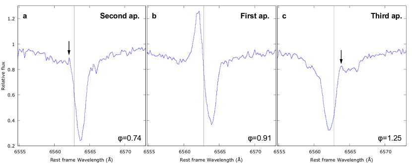
Figure 1: Comparison of the three apparitions of H$\alpha$ line profile of RR Lyr. Panel a: Second apparition at $\varphi=0.74$ represented with a spectrum dated on 2017-Apr-10. Panel b: First apparition at $\varphi=0.91$ represented with a spectrum dated on 2017-Apr-09. Panel c: Third apparition at $\varphi=1.25$ represented with a spectrum dated on 2017-Apr-08. Vertical line indicates the H$\alpha$ line laboratory wavelength.

We thus used the ephemerides provided by Le Borgne et al. (2014) for the aurelie and eShel II observations made in 2013 and 2014. For the 2017 data, a late epoch for the ephemeris provided by Le Borgne et al. (2014), the pulsation period $P_{P}$ was computed using the difference between the two closest $O-C$ minima from the GEOS RR Lyr web database and close to our 2017 observations. The reference HJD maximum light (HJD0_P) was also provided by this database. A summary of the ephemerides used for the different data sets is provided in Table 2.

The determination of the Blazhko phase is more problematic since the Blazhko period $P_{B}$ does not follow the variation in the pulsation period, but presents rather erratic changes (Le Borgne et al., 2014). Moreover, during 2014, the photometric $O-C$ were historically low (close to nil), preventing an easy Blazhko period computation.

Therefore, in order to find maximum light amplitude dates HJD0_B, we developed an innovative method, which will be described in a forthcoming paper (Gillet et al. in prep.), based on the equivalent width (EW) and main shock velocities driven by our many years of experience in performing spectral observations. For each photometric maximum ($\varphi=0$) corresponds to a spectroscopic maximum ($\varphi=0.91$) where H$\alpha$ presents an emission line. Consequently, —EW— and $|V_{\textrm{shock}}|$ (defined in Eq. 3) reach high values. They reach a maximum when the light amplitude $O-C$ correspond to their extrema, thus pointing out Blazhko maxima. We expect an uncertainty of $\pm 2$ days on HJD0_B and of $\pm 0.2$ d on $P_{B}$. Ephemerides were computed involving the period $P_{B}=39.0$ d (Le Borgne et al., 2014). A summary of the Blazhko ephemeris used for the different data set is provided in Table 2.

3 Observations of H$\alpha$ and sodium in RR Lyr

We analyzed profile variations for three spectral lines: H$\alpha$ , He, and Na D1 during a complete pulsation period. This last line is a resonance line that, following Fokin & Gillet (1997), is formed in the deep layers of the photosphere, while the core of the H$\alpha$ and helium lines are formed well above the photospheric layers, hereafter called the upper atmosphere. Thus, these three lines, by their different formation heights, are able to probe and to follow the propagation of the waves in the atmosphere along the pulsation cycle.

Because one observing night is not long enough to obtain spectra during the whole pulsation period ($P_{P}\simeq 13$ h 36 min), we had to recompose the data of 11 consecutive nights. It was shown by Gillet & Crowe (1988) that lines could vary depending on the Blazhko phase with a period of $P_{B}\simeq 39$ d. Thus, as 55 spectra out of 79 were obtained over three days, on this timescale the Blazhko effect must be secondary in the framwork of our data. Consequently, the use of data obtained in different periods will not change appreciably the different phases of the atmospheric dynamics and the effects of the shock wave propagation on these different phenomena, including their impact on the turbulence amplification.

3.1 H$\alpha$ line evolution

The three successive appearances of hydrogen emission (Preston, 2011) have been observed in detail. Between $\varphi=0.892-0.929$, just before the luminosity maximum, an intense blueshifted emission is present, the well-known “first apparition.” A smaller red bump is detectable from $\varphi=0.637$ to $\varphi=0.736$. Panel a of Fig. 1 zooms in on this “second apparition,” which is the weak hump at the top of the blue line wing around $\varphi\approx 0.73$. Finally, another small red bump corresponding to the “third apparition” is detected for $\varphi=0.181-0.387$. These three apparitions are compared in Fig. 1. While only one line profile is plotted for each apparition in this figure, they are observed in several consecutive spectra (see Figs. 2 and 3).

The blueshifted emission intensity corresponding to the first apparition (Fig. 1, panel b) represents up to 30% of the continuum, depending on the Blazhko phase. The duration of the emission of the H$\alpha$ line for the first apparition is between 15 min and 40 min, i.e., less than 5% of the pulsation cycle. This phenomenon is rather short compared to the second and third apparitions (Fig. 1 panels a and c, respectively). Their durations are respectively about 1.5 h and 3 h, i.e., 11% and 20% of the pulsation period.

The second apparition was first observed in RR Lyr by Gillet & Crowe (1988). They measured a 30 min duration in nonconsecutive observations. This emission may depend on the pulsation cycle and requires observations over several cycles to be clearly defined.

On the other hand, the third apparition was first reported in RR Lyr itself by Gillet et al. (2017), where the emission intensity and duration are consistent with our observations. However, these two apparitions intensities represent only a few percents of the continuum.

Figures 2 and 3 show the evolution of the H$\alpha$ line profile over the full pulsation cycle. They start at the bottom left and go toward the top right. The H$\alpha$ line becomes redshifted at $\varphi=0.618$. It is followed by a line doubling starting at $\varphi=0.943$ and ending at $\varphi=1.027$, i.e., $\sim 8\%$ of the pulsation cycle. Then the H$\alpha$ line remains blueshifted until $\varphi=1.461$, where it reaches its laboratory wavelength, and then becomes redshifted again. The shock intensity depends on the Blazhko phase: the more important it is, the more visible the He I emission lines become.

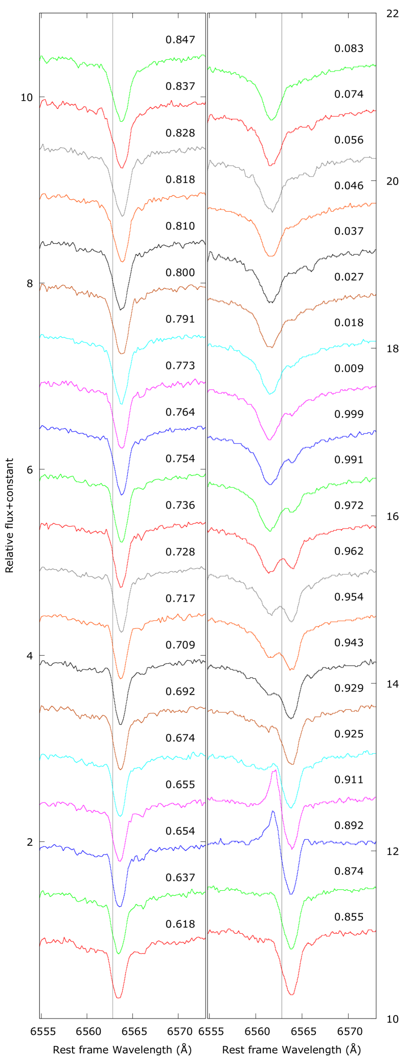
Figure 2: Evolution of the H$\alpha$ line profile based on RR Lyr observations obtained in April 2017. The pulsation phase varies from $\varphi=0.618$ (bottom left) to $\varphi=0.083$ (top right), while the Blazhko phase $\psi$ overlays the interval 0.77-0.03. The exposure time is 900 s, but the time step is shorter. Weak absorption features are telluric lines. The vertical line indicates the H$\alpha$ line laboratory wavelength.

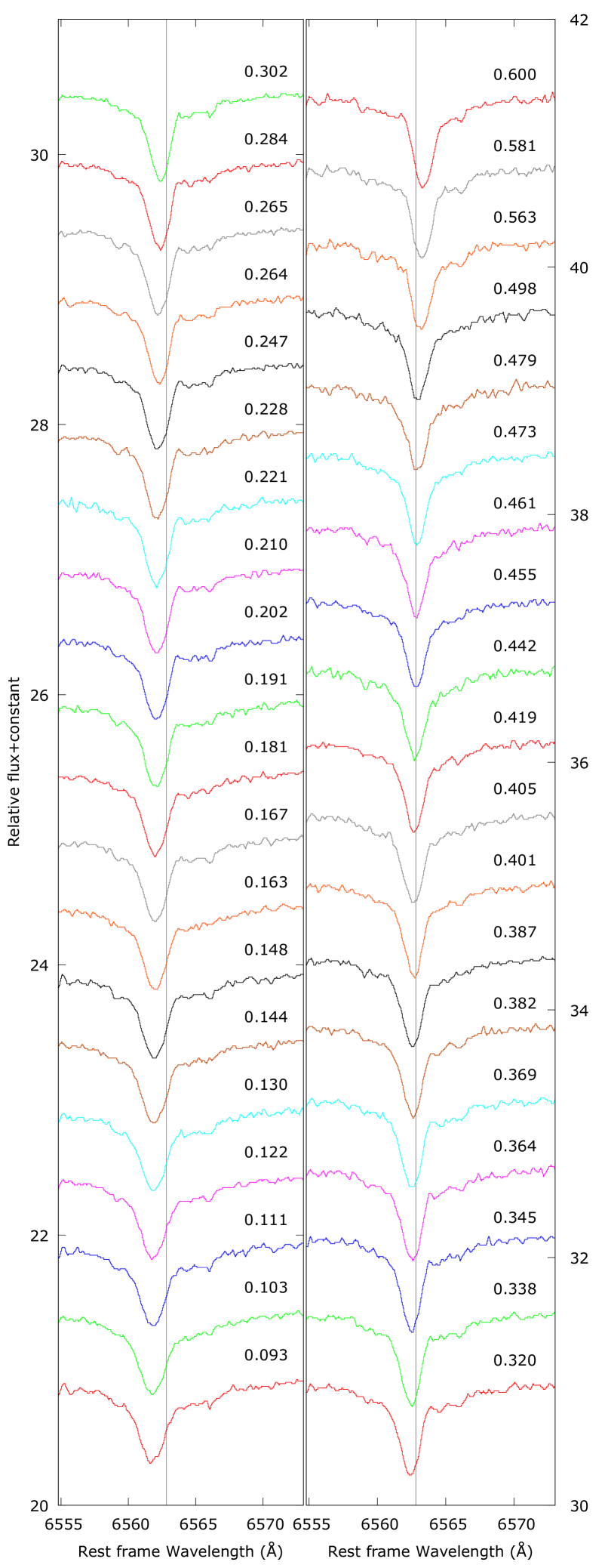
Figure 3: Evolution of the H$\alpha$ line profile based on RR Lyr observations obtained in April 2017. The pulsation phase varies from $\varphi=0.093$ (bottom left) to $\varphi=0.600$ (top right), while the Blazhko phase $\psi$ overlays the interval 0.77-0.03. The exposure time is 900 s, but the time step is shorter. Weak absorption features are telluric lines. The vertical line indicates the H$\alpha$ line laboratory wavelength.

3.2 Helium line evolution

Figure 4 shows the He I $\lambda 5876$ line in emission at $\varphi=0.911$, i.e., the same phase of the first apparition of the H$\alpha$ line. This emission was first reported in RR Lyr by Gillet et al. (2013). Its intensity is 8% of the continuum and the line velocity reaches $-6.5\pm 0.8$ km s^-1 , which confirm the Gillet et al. (2013) measurements. While this emission is a short phenomenon of less than 30 min, i.e., $\sim 3$% of the pulsation period, it is followed by an absorption shape between $\varphi=0.925-0.954$. We note that the low value $\textrm{S/N}_{\textrm{He line}}\cong 3$ prevents us from performing a more detailed analysis of such a weak feature. No emission of the He I $\lambda 6678$ line is observed at the same phase. This is consistent with the Blazhko phase $\psi=0.77$ for this observation on the night of April 8–9, 2017. Indeed, this Blazhko phase corresponds to a strong shock, but not an exceptional one. Stronger shocks are expected around $\psi=0$ (Gillet, 2013).

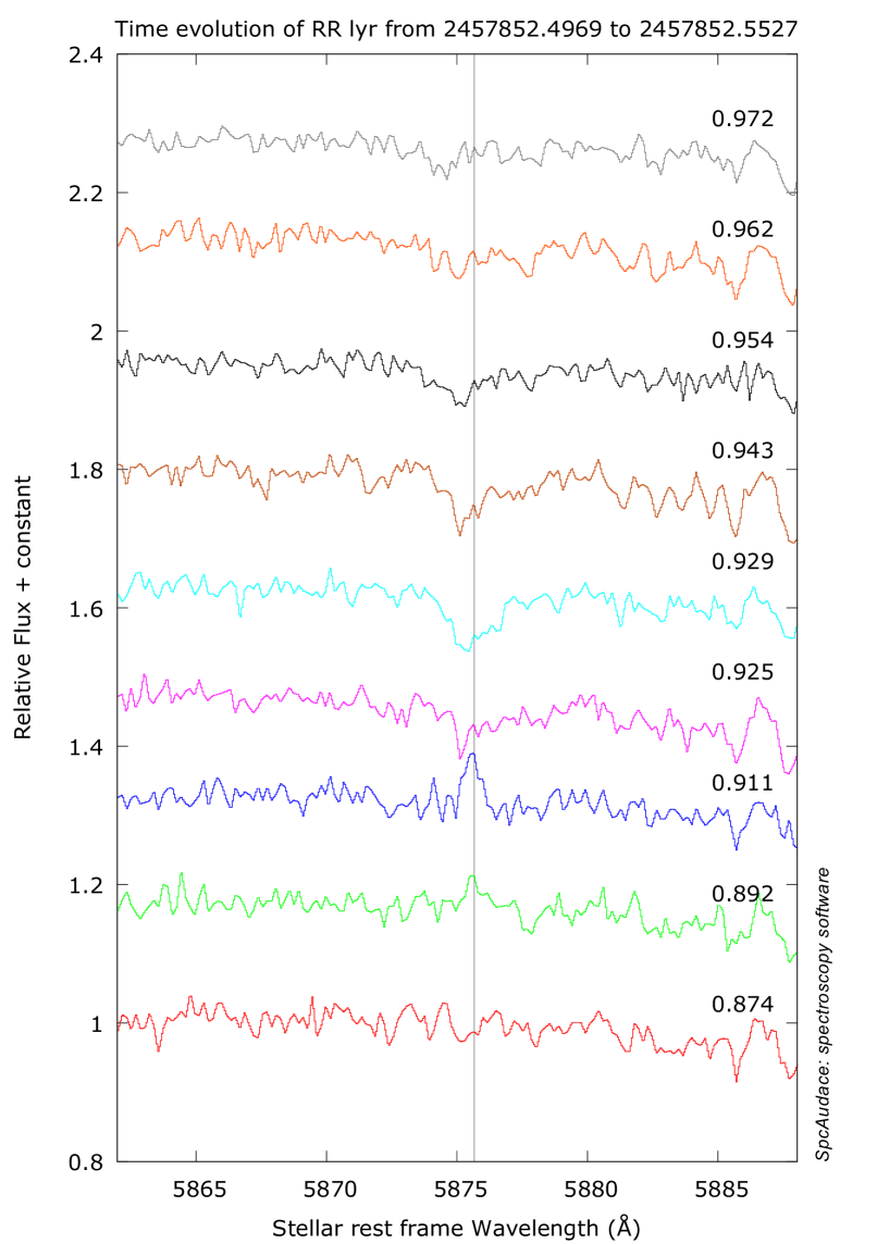
Figure 4: Apparition of the He I $\lambda 5876$ emission line at $\varphi=0.911,$ i.e., when the H$\alpha$ line is also in emission. The vertical line indicates the He I line laboratory wavelength.

3.3 Sodium line evolution

Figures 5 and 6 show the evolution of the D1 sodium line profile ($\lambda$5895.92) over the full pulsation cycle. Two strong telluric lines are blanketing the center of the D2 sodium component at $\lambda 5889.95$ line (Hobbs, 1978). Consequently, we focused our analysis on the D1 sodium component at $\lambda$5895.92 line. This line is denoted Na D in the paper. Figures 5 and 6 show the evolution of the D1 line profile over the full pulsation cycle.

A line doubling starts somewhere for $\varphi\in[0.892;0.925]$, i.e., very close to the pulsation phase of the first apparition of the H$\alpha$ line. It remains visible along $\varphi\in[0.855;1.600]$, i.e., over 75% of the pulsation cycle. The origin and evolution of these two components of the D1 line profile are analyzed in detail in Sects. 4 and 5.

3.4 Line velocity evolution

From the whole time series composed of 79 spectra, we selected 19 spectra that led us to describe every step of the layer motion evolution during one pulsation cycle. In order to probe atmospheric dynamics we extracted the radial velocities of the sodium and the H$\alpha$ absorption lines. Measurements were done with respect to the stellar rest frame. Line center measurements were obtained by Gaussian fitting or first moment of the line profile, depending on the line shape. The mean uncertainty is $\pm 0.6$ km s^-1. These Doppler velocities are listed in Table 3 and presented in Fig. 7 where curves are computed with a cubic spline.

The sodium blueshifted component has a very perturbed behavior, alternating receding and ascending movements. However, the redshifted velocity component remains constant around 50 km s^-1. A detailed analysis is presented in Sect. 4.

Table 3: Radial velocity measurements with respect to the stellar rest frame of sodium and H$\alpha$ absorption lines within the pulsation phase. The mean uncertainty computed from line center measurements is $\pm 0.6$ km s^-1.

Phase	Line velocity (km s-1)
$\varphi$	Na (blue)	Na (red)	$\textrm{H}\alpha\textrm{ (abs)}$
$0.874$	$+25.0$	$+45.4$	$+46.9$
$0.892$	$+10.1$	$+47.8$	$+44.9$
$0.911$	$-11.5$	$+50.1$	$+46.9$
$0.943$	$-24.1$	$+49.8$	$-58.5\leavevmode\nobreak\ \leavevmode\nobreak\ +43.3$
$0.991$	$-31.3$	$+49.5$	$-60.6\leavevmode\nobreak\ \leavevmode\nobreak\ +48.5$
$1.027$	$-25.8$	$+48.6$	$-63.2\leavevmode\nobreak\ \leavevmode\nobreak\ +49.8$
$1.074$	$-24.3$	$+49.7$	$-52.3$
$1.202$	$-13.4$	$+48.8$	$-34.9$
$1.302$	$-2.7$	$+50.5$	$-21.1$
$1.320$	$+0.1$	$+48.5$	$-18.8$
$1.401$	$+6.7$	$+49.0$	$-7.2$
$1.455$	$+10.2$	$+49.6$	$-0.2$
$1.473$	$+13.6$	$+50.8$	$+2.9$
$1.498$	$+14.1$	$+48.5$	$+5.7$
$1.581$	$+20.9$	$+49.3$	$+19.1$
$1.600$	$+24.1$	$+49.8$	$+23.3$
$1.618$	+34.9		$+27.8$
$1.754$	+33.2		$+42.5$
$1.810$	+37.1		$+41.9$

Like all spectral lines, the H$\alpha$ absorption line evolution alternates ascending and receding movements over the whole pulsation cycle. Near $\varphi=0.892$, the first emission arises. This is followed by a brief line doubling episode ($\varphi=0.943-1.027$), during which the extremal blue ($B$) and red ($R$) radial velocities of these two components are $V(H\alpha_{B})=-63.2$ km s^-1 and $V(H\alpha_{R})=+49.8$ km s^-1. At $\varphi=1.037$, the H$\alpha$ line starts a progressive redshift from its maximum blueshifted velocity value $-54.6$ km s^-1 to finish at $+46.9$ km s^-1 near $\varphi=1.874$. The H$\alpha$ line dynamics is studied in detail in Sect. 4.

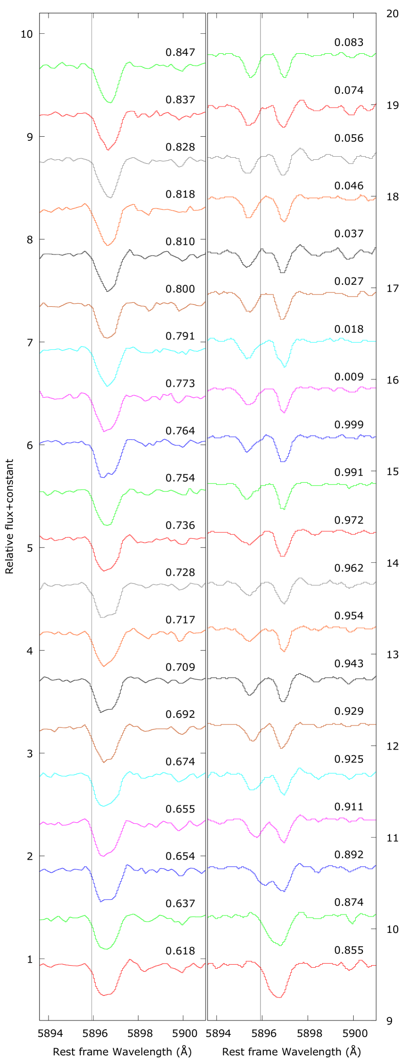
Figure 5: Evolution of the D1 sodium line profile ($\lambda$5895.92) based on RR Lyr observations obtained in April 2017. The pulsation phase varies from $\varphi=0.618$ (bottom left) to $\varphi=0.083$ (top right), while the Blazhko phase $\psi$ overlays the interval 0.77-0.03. The exposure time is 900 s, but the time step is shorter. There is a line doubling that stays over 75% of the cycle. The vertical line indicates the sodium line laboratory wavelength.

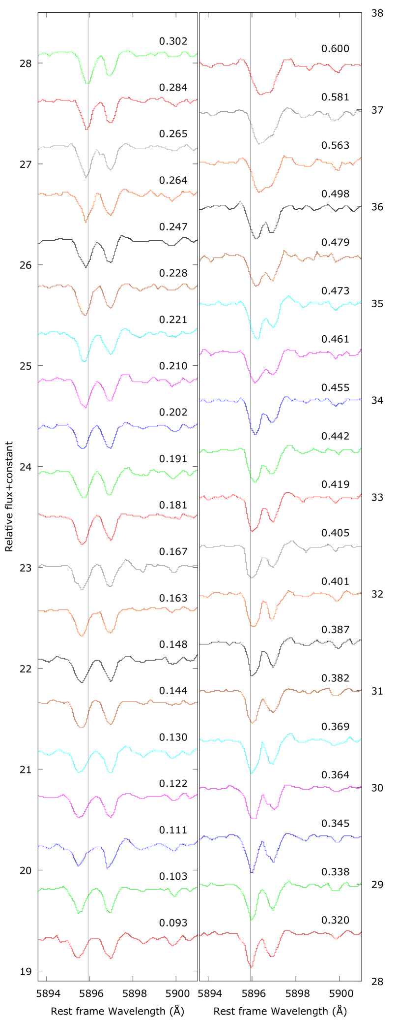
Figure 6: Evolution of the D1 sodium line profile ($\lambda$5895.92) based on RR Lyr observations obtained in April 2017. The pulsation phase varies from $\varphi=0.093$ (bottom left) to $\varphi=0.600$ (top right), while the Blazhko phase $\psi$ overlays the interval 0.77-0.03. The exposure time is 900 s, but the time step is shorter. There is a line doubling which remains over 75% of the cycle. The vertical line indicates the sodium line laboratory wavelength.

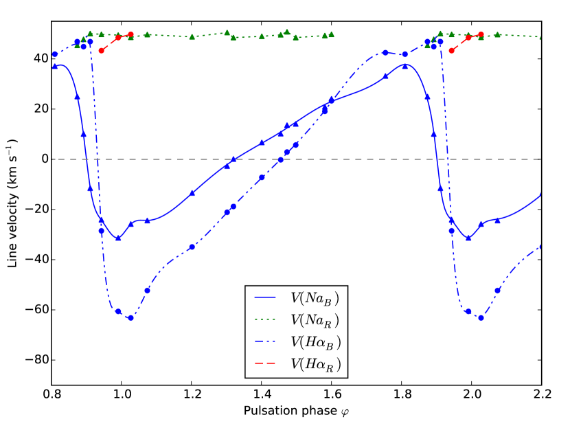
Figure 7: Curves of velocity with respect to the stellar rest frame of the sodium and H$\alpha$ over the pulsation phase $\varphi=0.8$ to $\varphi=2.2$. Shown are the blue components, $V(Na_{B})$ (blue filled line) and $V(H\alpha_{B})$ (blue dot-dashed line), and their respective red components, $V(Na_{R})$ (green dotted line) and $V(H\alpha_{R})$ (red dashed line). The mean uncertainty is $\pm 0.6$  km s^-1.

4 The very redshifted sodium component

Our observations (Figs. 5 and 6) show that a very redshifted component is present within the Na D line profiles near $\lambda$5897. It is clearly visible from $\varphi=0.911$ to $\varphi=0.302$, i.e., when it is not blended with the variable pulsational sodium component. Between 1994 and 2017, its velocity remains constant near $+50.3\pm 1.2$ km s^-1 (see Table 4). The shape of this component also seems constant, i.e., it is not dependent on the pulsation phase. However, the line profiles of other metallic lines such as Fe ii $\lambda 4923.921$ and Mg i $\lambda 5183.604$ (Chadid & Gillet, 1996) as well as Balmer lines (Preston et al., 1965) observed at a resolving power of up to $R=44\,000$ do not present such a very redshifted component as observed for Na D lines. This points toward a nonphotospheric origin of this very redshifted Na D line component.

Table 4: Measurements of the very redshifted component within the Na D line profiles: $V_{\textrm{radial}}$ by Gaussian fitting with respect to the stellar rest frame, FWHM corrected from instrument function, and EW at $\varphi=0.000-0.083$ from the 1994 – 2017 spectra.

Date	$\varphi$	$V_{\textrm{radial}}$	FWHM	EW
(yyyy-mm-dd)		$(\textrm{km\,s}^{-1})$	$(\mbox{\AA})$	$(\mbox{\AA})$
1994-08-03	$0.083$	$49.3$	$0.168$	$0.1554$
1996-08-02	$0.083$	$50.6$	$0.189$	$0.1541$
1997-06-03	$0.083$	$50.2$	$0.154$	$0.1580$
1997-08-05	$0.083$	$51.2$	$0.199$	$0.1565$
1997-08-09	$0.083$	$51.7$	$0.205$	$0.1558$
1997-08-31	$0.083$	$50.7$	$0.166$	$0.1652$
2013-10-16	$0.083$	$51.5$	$0.160$	$0.1443$
2014-05-01	$0.008$	$50.4$	$0.197$	$0.1686$
2016-07-18	$0.005$	$48.4$	$0.206$	$0.1652$
2017-05-17	$0.034$	$48.5$	$0.171$	$0.1543$
Mean & RMS	$-$	$50.3\pm 1.2$	$0.182\pm 0.018$	$0.1577\pm 0.0070$

The maser emissions SiO or OH are considered as proof of the presence of a circumstellar envelope. Nevertheless, until now this type of emission has never been detected for RR Lyr. In addition, microwave CO lines, which could be the fossil remnants of an ancient shock ejection, have not been detected. Moreover, RR Lyr is not known to have strong mass loss due to spectacular shock ejections like those occurring in unstable red giant envelopes (Tuchman et al., 1978, 1979). As a result, it is unlikely that RR Lyr has a circumstellar envelope. The most likely explanation of this redshifted component is an interstellar medium (ISM) origin. It would be due to the absorption by interstellar dust and gas on the line of sight of RR Lyr.

The sodium splitting is seen in only 75% of the pulsation cycle, but not in the other 25%. The stellar component merges with the static ISM component during $\varphi$ interval $0.563-0.874$ since the Na stellar component is redshifted at $\varphi=0.338-0.892$.

The corresponding large observed heliocentric velocity ($V_{\rm helio}=+50.3-73.5=-23.2$ km s^-1 , where $V_{\ast}=-73.5$ km s^-1) of the redshifted component is consistent with an interstellar origin because, as RR Lyr has a low galactic latitude ($b=12$ ^∘), the radial velocity of the expected interstellar material could be large due to small projection effect. The observed FWHM of the red component remains approximately constant between 1994 and 2017 around $0.182\pm 0.02$ Å, i.e., $9.3\pm 0.9$ km s^-1 (see Table 4). This line width corresponds to the sum of a thermal part and a turbulent part occurring within the ISM gas. It is consistent with the FWHM observed on the high-resolution spectral profiles of the interstellar Na I D line toward 80 early-type stars located in the local interstellar medium (Welsh et al., 1994).

According to the GAIA database, RR Lyr has a parallax of $3.64\pm 0.23$ mas, i.e., a distance of 895 light-years (ly) (Gaia Collaboration et al., 2016). The Sun is located in a low-density region of the interstellar medium (about 0.05 atoms per cubic centimeter of neutral hydrogen, a near-perfect vacuum) called the Local Bubble (Frisch et al., 2011). This gigantic asymmetric cavity of 330 to 490 ly in diameter has a wall of denser matter at its surrounding. It is believed that the Local Bubble has been carved by fast stellar winds and supernova explosions within the last 10 Ma. Consequently, this cavity is partially filled with hot gas. RR Lyr is located in another expanding cavity called Loop III (Kun, 2007). Between them, at about 200 ly from RR Lyr, Loop III and the Local Bubble are separated by a wall of about 150 ly in size, of colder and denser neutral gas. Because the gas density within the cavities is at least 10 times lower than the average ISM density of the rest of the Milky Way’s spiral disk, we can expect that the very redshifted sodium component is formed within the Local Bubble wall.

Gillet et al. (2017) have performed a single observation (2017-03-26) of the sodium line at $\varphi=0.227$. The profile shows a line doubling. Because the two components are similar (same FWHM and depth) it was thought that they were formed in a same atmosphere. Consequently, Gillet et al. (2017) suggested that the sodium doubling at $\varphi=0.227$ is due to the presence of a shock within the RR Lyr atmosphere. In the present paper we present a series of 79 spectra sampled approximately every 15 min over the whole pulsation cycle, so we are able to show that the radial velocity of this component, when it is clearly visible, remains stable during the whole pulsation cycle for all line profile parameters. Consequently, we suggest that the redshifted component of the sodium profile has an interstellar origin. As a result, there would be no large velocity ($+50.3\pm 1.2$ km s^-1) sodium layer falling on the atmosphere around the pulsation phase $\varphi\sim 0.30$, which would enhance the atmospheric compression causing the appearance of the third H$\alpha$ emission.

5 Dynamical structure of the atmosphere

The pulsation of RR Lyr concerns essentially the photosphere and the atmospheric layers, which represent only a small percent of the mass of the star.

Here we consider the main dynamic phenomena occurring during a pulsation period of RR Lyr of average amplitude. It is assumed to take place about halfway between the minimum and the maximum Blazhko, i.e., around the Blazhko phase $\psi=0.75$. The pulsation amplitude is minimum at Blazhko minimum and maximum at Blazhko maximum. The amplitude gradually increases between Blazhko minimum and Blazhko maximum. However, it is known that appreciable fluctuations are observed from one cycle to another. The Kepler-amplitude $K_{p}$ of the light curve of RR Lyr (see Figs. 2 and 3 in Gillet 2013), which is correlated to the intensity of the main shock, strongly depends on the previous pulsation cycle. As a result, this random behavior induces appreciable effects on the atmospheric dynamics, such as changes in observed line profiles. For example, helium lines can be in emission or not. Apart from these fluctuations, observations and models show that the dynamics of the pulsation follows a general reproducible scenario from one cycle to another. In this section we decompose these atmospheric phenomena into six main steps that characterize the different dynamic processes occurring during a pulsation cycle (see Table 5).

Table 5: Decomposition of phenomenological steps of RR Lyr atmospheric dynamics during a typical pulsation cycle (see Sect. 3).

Step	$\varphi\ \mathrm{interval}$	Phenomenon
1	$0.874-0.892$	Emergence of the main shock
2	$0.892-0.929$	Radiative shock wave phase
3	$0.320$	Maximum expansion of the sodium layer
4	$0.455$	Maximum expansion of the H$\alpha$ layer
5	$0.320-0.455$	A two-step infalling motion
6	$\mathrm{around\ 0.36}$	A strong phostospheric compression

5.1 Phase 1 (0.874-0.892): emergence of the main shock

Near the pulsation phase $\varphi=0.89$, a blueshifted H$\alpha$ emission component suddenly appears within the H$\alpha$ profile (Fig. 2). When the H$\alpha$ emission reaches its maximum intensity ($\varphi=0.911$), He i and H ii lines can also be in emission if the light curve amplitude, hence the main shock, is large enough. Helium emission lines are not easily observed because their intensity is low (Fig. 4). Consequently, their exhaustive detection requires spectra with a high S/N, i.e., the use of large-diameter telescopes.

As noted in the introduction, RR Lyrae models that consider an atmosphere and shocks are rare. Fokin & Gillet (1997) presented in detail two models of RR Lyr that give the same fine atmospheric structure (see Appendix A). At the end of the global compression of the star near the phase $\varphi=0.80$, the $\kappa-\gamma$ mechanism associated with the H-ionization zone provokes a local overpressure, followed by the generation of a wave w1 that quickly breaks into the shock wave s1. At approximately the same phase the second helium ionization zone, which is located far below the photosphere, also generates by a similar mechanism, a compression wave w2 which quickly turns into the shock wave s2.

As shown by Fokin & Gillet (1997), these two waves propagate first toward the interior of subphotospheric layers. In approximately the phase interval 0.75-0.90, the whole atmosphere falls on the star with an infall velocity exceeding that of the waves. Thus, all waves (or shocks) are first receding for the observer (Eulerian coordinates), but their motion is expanding outward in the Lagrangian frame. After phase 0.90, the Mach number of shocks becomes as high as 15–25 and with the deceleration of the atmosphere during its downward motion, the shock starts to propagate outward in the Eulerian frame.

From the sodium and H$\alpha$ line profiles reported in this paper (see Figs. 3, 2, 5, and 6), it is not possible to distinguish independently the shock waves s1 and s2. Since the latter are formed well below the photosphere ($T\sim 40,000$ K), the optical depth is certainly too large for the H$\alpha$ profile to be affected.

5.2 Phase 2 (0.892-0.929): the shock is radiative

For the observations presented in this paper, an H$\alpha$ emission occurs at the pulsation phase $\varphi=0.892$. The emission is visible during a short time interval from $\varphi=0.892$ to $\varphi=0.929$, i.e., during 5% of the pulsation cycle. The intensity of the shock is thus important enough to produce emission lines: it is a radiative shock.

The H$\alpha$ emission is formed just behind the shock front within the radiative shock wake. This region is very narrow, typically a few kilometers depending on the shock velocity and physical condition within the atmosphere (Fadeyev & Gillet, 2004). At what velocity (or Mach number) does the shock become radiative?

At $\varphi=0.892$, the emission is blueshifted (and defined by $V_{e1}=-44.4$ km s^-1, Fig. 2). It is possible to obtain an estimate of the shock front velocity from the velocity of the blueshifted H$\alpha$ emission. The gas layers emitting the Balmer line radiations are located at the rear of the shock front in the hydrogen recombination zone. We use shock models of Fadeyev & Gillet (2004), which consider the structure of steady-state plane-parallel radiative shock waves propagating through a partially ionized hydrogen gas of pre-shock temperature $T_{1}=3\,000$ K and pre-shock densities between $\rho_{1}=10^{-9}$ g cm^-3 and $10^{-12}$ g cm^-3. Thus, in the frame of the observer, the gas flow velocity in the hydrogen recombination zone is roughly one-half of the shock wave velocity:

$$\frac{V_{\textrm{shock}}}{V_{\textrm{recomb}}}\cong 2.00\pm 0.11$$ (1)

From these models it is also possible to estimate the ratio of $V_{e1}$ (denoted $\delta V$ in Fadeyev & Gillet 2004) of the hydrogen first emission component Doppler shift to the gas flow velocity $V_{\textrm{recomb}}$ in the hydrogen recombination zone:

$$\frac{V_{e1}}{V_{\textrm{recomb}}}\cong 0.70\pm 0.03$$ (2)

Combining these two equations, we obtain

$$V_{\textrm{shock}}(\varphi\simeq 0.90)\cong 3V_{e1}\cong 3c\frac{(\lambda_{e1}-\lambda_{0})}{\lambda_{0}}\,\pm 0.16V_{\textrm{shock}},$$ (3)

where $\lambda_{e1}$ is the wavelength of the maximum intensity ($\varphi\simeq 0.90$) of the H$\alpha$ emission and $\lambda_{0}$ its laboratory wavelength. Since during the first apparition (pulsation phase $\varphi\sim 0.91$) the emission line is blueshifted, then $V_{\textrm{shock}}<0$ and the shock wave is coming toward the observer. However, for practical purpose we use the absolute value of $V_{\textrm{shock}}$ in this paper. The uncertainties of Eqs. 1, 2, and 3 were estimated from the values given in Table 1 of Fadeyev & Gillet (2004) for the different shock velocities and atmospheric densities. For the considered shock wave model, the validity of Eq. 3 is verified for shock velocities from 40 km s^-1 to 90 km s^-1 , i.e., for Mach numbers ranging from 6.2 to 14.

If we apply this equation to the observed H$\alpha$ line profile in the pulsation phase interval $0.89-0.93$ (Figure 2), we obtain an estimate of the shock front velocity. We derive the H$\alpha$ emission position by Gaussian fitting or first moment method depending on the line shape. Velocity uncertainties, which are much larger than measurements uncertainties, are computed with Eq. 3 estimated from the Fadeyev & Gillet (2004) models. Since the emission line is blueshifted for the first apparition, the shock intensity, i.e., the absolute value of $V_{\textrm{shock}}$, is considered for the clarity of the analysis. Most of measurements come from the night of 2017-04-09. In order to improve the time resolution, we added an observation from the night of 2017-04-12, which corresponds to $\varphi=0.925$, assuming that shock velocity does not vary too much between consecutive pulsation cycles. This assumption is verified because the measured shock velocity at this phase ($+111$ km s^-1) is an intermediate value between $+108$ km s^-1 and $+158$ km s^-1. Theses values are listed in Table 6.

Table 6: Doppler velocity of H$\alpha$ emission line with respect to the stellar rest frame, $|V_{\textrm{shock}}|$, and Mach number value within the pulsation phase for the 2017-Apr-08 observation night ($\psi=0.77$) as defined by Eq.3. Uncertainties are computed with Eq.3 estimated from Fadeyev & Gillet (2004) models and are much larger than measurement uncertainties.

$\varphi$	$V_{e1,\alpha}$	$|V_{\textrm{shock}}|$	${\rm Mach}$
	$(\textrm{km\,s}^{-1})$	$(\textrm{km\,s}^{-1})$	${\rm number}$
$0.892$	$-44.4\pm 0.6$	$133\pm 21$	$13$
$0.911$	$-39.3\pm 0.6$	$118\pm 19$	$12$
$0.925$	$-37.0\pm 0.6$	$111\pm 18$	$11$
$0.929$	$-36.0\pm 0.6$	$108\pm 17$	$11$

With an assumed sound velocity of $10$ km s^-1, the Mach number is between 11 and 13. Thus, with physical conditions present in the atmosphere of RR Lyr, the shock becomes radiative for $M\gtrsim 10$.

The average shock front velocity is around $120$ km s^-1 (see Table 6). This value is much greater than the expected maximum velocity of $+40$ km s^-1 of the infalling atmosphere (see Fig. 7 near $\varphi=0.82$). Our estimate of the shock front velocity is thus consistent with the hypothesis that the intensity of the shock wave must be intense enough to reverse the supersonic infall motion of the sodium layer.

Our observations of the hydrogen emissions were made on the night of April 8, 2017. The corresponding Blazhko phase is $\psi=0.77$, i.e., almost halfway between the minimum and the maximum Blazhko. This must explain why the observed shock velocity (from $133$ to $108$ km s^-1; see Table 6) is relatively moderate in contrast to those which can occur at maximum Blazhko, up to $\simeq 170$ km s^-1 (Gillet et al., in prep.).

The question is whether the Eq. 3 used in this paper can be applied to velocities as high as 110 km s^-1 or even higher. When the shock velocity increases, the hydrogen gas behind the shock front is rapidly fully ionized. Moreover, the optical thickness at the H$\alpha$ central wavelength decreases when the shock velocity increases. Thus, the radiative cooling of the gas increases. In the limit case of very efficient cooling, the isothermal approximation can be made: the cooling is assumed to be instantaneous. Thus, the gas returns to its original pre-shock temperature ($T_{1}$) just behind the shock front: $T_{2}=T_{1}$. This means that the cooling time is very short compared to the dynamic time of the shocked atmosphere.

However, as shown by Fadeyev & Gillet (2004), for photospheric densities and with a shock front velocity of 90 km s^-1, the compression rate within the hydrogen recombination zone only reaches a small percent of the isothermal case. Due to the lack of shock models with front velocities up to 200 km s^-1, we can only assume that the approximate Eq. 3 remains valid in the radiation flux-dominated regime.

Finally, we find that in the phase interval $\varphi=0.892-0.929$ the shock velocity decreases all the time. Consequently, the observations do not show any acceleration phase of the shock, but only its deceleration phase in the atmosphere. The acceleration phase of the shock necessarily occurs between the moment when the compression waves w1 and w2 are created by the $\kappa-\gamma$ mechanism and the beginning of the deceleration phase of the shock.

5.3 Phase 3 (0.320): maximum expansion of the sodium layer

From Table 3, the photospheric sodium component (blue component) reaches a velocity maximum of $-31.3$ km s^-1 at $\varphi=0.991$ after a continuous velocity increase from $\varphi=0.911$. After $\varphi=0.911$, the velocity continually decreases. This means that, contrary to the H$\alpha$ layer where the H$\alpha$ blueshifted absorption is produced, the sodium layer first accelerates before decelerating from $\varphi=0.911$.

At $\varphi=0.320$, the sodium layer stops its ascending motion and starts its slowly infalling motion. The sodium layer thus reaches its maximum expansion in the atmosphere at $\varphi=0.320$, while the H$\alpha$ layer, where the H$\alpha$ absorption is formed, is still ascending. The sodium and H$\alpha$ layers have now an opposite motion and consequently, from this time, an increasing rarefaction zone appears in the atmosphere.

The generation of rarefaction and compression waves during the development of the pulsation of the atmosphere have already been theoretically demonstrated by Hill (1972). Thus, it appears that the motion of the photospheric layers is rather complicated when a layer reverses its movement in relation to another.

5.4 Phase 4 (0.455): maximum expansion of the H$\alpha$ layer

After the end of the H$\alpha$ line doubling ($\varphi=0.027$), the H$\alpha$ profile is in absorption and single. Its radial velocity begins to rapidly decrease from $\varphi=0.074$ ($-52.3$ km s^-1) to $\varphi=0.455$ where its value reaches $\sim 0$ km s^-1 (Table 3 and Fig. 3). Consequently, at $\varphi=0.455$, the H$\alpha$ line-forming region stops its expansion. At $\varphi=0.473$, the H$\alpha$ absorption line becomes redshifted (Fig. 3). Thus, this part of the atmosphere begins to reverse its movement toward the center of the star.

During the ascension end of the sodium layer, which was driven by the shock now located just above it, the radial velocity of the H$\alpha$ blueshifted component continues to decrease slowly (from -21.1 km s^-1 to -18.8 km s^-1) as described in Table 3. This means that the expansion of the H$\alpha$ layer located just behind the shock front is not yet complete. The H$\alpha$ profile is now in absorption and single. Its radial velocity continues to decrease to $\sim 0$ km s^-1 at $\varphi=0.455$ (Table 3 and Fig. 3). At $\varphi=0.473$, the H$\alpha$ absorption line becomes redshifted (Fig. 3). Thus, this part of the atmosphere begins to reverse its movement toward the center of the star.

5.5 Phase 5 (0.320-0.455): a two-step infalling motion

During the phase interval $0.320\lesssim\varphi\lesssim 0.455$ the sodium line is redshifted. As a result, the lower atmosphere, where the sodium component is produced, begins its infalling movement well before ($\varphi=0.320$) that of the atmosphere in which the H$\alpha$ line is formed ($\varphi=0.473$). It is necessary to wait for 15% of the pulsation period for the hydrogen layer to begin to fall on the star.

Our observations show that the atmospheric layers do not follow a synchronized ballistic movement even in the lower part of the atmosphere. It is the propagation of the radiative (hypersonic) shock wave that causes this strong desynchronization of the pulsation movement. If we limit our observational analysis to the movement of the layers of sodium and hydrogen, we have an infalling movement in two successive steps. This means that during the phase interval $0.320\lesssim\varphi\lesssim 0.455$, the sodium and H$\alpha$ layers, which are localized behind the shock, have opposite movements within the atmosphere.

Finally, it is expected that when a shock of large amplitude (hypersonic) occurs within a pulsating atmosphere, a strong desynchronization of the layer motions takes place in the atmosphere. It should be easy to validate this statement using high-resolution spectroscopic observations.

5.6 Phase 6 ($\sim 0.36$): a strong photospheric compression

From our observations presented in a previous paper (Gillet et al., 2017), the H$\alpha$ third emission line is observed approximately within the phase interval $0.20\lesssim\varphi\lesssim 0.40$. Due to the variation between pulsation cycles, the duration range of visibility of the third emission may undergo some variations on the order of 5% to 10% in the pulsation phase. In all cases, the presence of a third emission line indicates that a strong warming occurs in the atmosphere due to the intense compression induced by the infalling layers.

Due to the new pulsation cycle, as shown by the model, at $\varphi=0.20$ the whole atmosphere located behind the shock wave is expanding. Only the highest layers of the atmosphere that have not yet been traversed by the shock are still falling back on the star. The ballistic motion of these layers was induced by the previous pulsation cycle.

From our observations we find that the H$\alpha$ line-forming region stops its expansion at $\varphi=0.455$. Because the third H$\alpha$ emission disappears near $\varphi=0.40$, this means that the ascending H$\alpha$ region contributes all the time to the compression, inducing the H$\alpha$ third emission line. On the other hand, this is not always the case of the sodium layer because it begins its infalling movement at $\varphi=0.320$.

The maximum intensity of the H$\alpha$ third emission should correspond to the maximum of the compression. For our observations made during the night of 2014-09-14 (Gillet et al., 2017), the maximum compression probably occurs around the pulsation phase $\varphi=0.357$. Thus, the most intense part of the compression occurs after the beginning of the infalling motion of the sodium layer.

The atmospheric phenomena and the shock wave behavior are summarized in Table 7.

Table 7: Shock wave, and Na and H$\alpha$ layer movements in stellar rest frame during a typical pulsation cycle of RR Lyr , as described in Sect. 4. The given phase values may vary to within a few hundredths because the temporal reproducibility of the cycles is variable.

$\varphi\ \mathrm{interval}$	Na movements	H$\alpha$ movements	Shock wave
$0.874-0.90$	Up to about $\varphi=0.90$, the Na layer is receding. When it is traversed by the shock, it reverses its motion and starts an ascending motion in the atmosphere.	Highest layer receding at an average velocity near $+46$ km s-1	s1 and s2 shock waves are initiated below photosphere, but are not observed individually. When above the photosphere, the main shock (s1+s2) is crossing the Na layer.
$0.90-0.943$	Ascending acceleration from 0 to $-24$ km s-1	Highest layer receding at $+46$ km s-1 throughout this phase interval and deepest layer ascending (producing emission in shock wake)	Deceleration of the main shock from $133$ to about $100$ km s-1. First apparition of H$\alpha$ emission ($0.892\lesssim\varphi\lesssim 0.911$).
$0.943-1.074$	The Na layer reaches its maximum ascending velocity ($-31.3$ km s-1) at $\varphi=0.991$	Ascending deceleration from $-58$ to $-63$ km s-1. Short line doubling ($0.953<\varphi<1.027$)	Deceleration of the main shock followed by disappearance (radiative dissipation). The main shock leaves the H$\alpha$ layer around $\varphi=1.05$.
$1.074-1.302$	Ascending deceleration from $-24$ to $0$ km s-1. The Na layer reaches its maximum radius.	Ascending deceleration from $-52$ to $-21$ km s-1	The main shock has left the H$\alpha$ formation layer.
$1.302-1.320$	Maximum expansion of Na layer	The highest part of the H$\alpha$ layer is still ascending.	The main shock has left the atmosphere. Apparition of the third H$\alpha$ emission ($0.20\lesssim\varphi\lesssim 0.40$) induced by the compression of the high atmosphere.
$1.320-1.455$	Receding acceleration from $0$ to $+10$ km s-1. Two-step infalling motion. Strong compression of deep photospheric layers at $\varphi\sim 0.36$	Ascending deceleration from $-19$ to $0$ km s-1. Maximum expansion of H$\alpha$ layer.	The main shock has left the atmosphere.
$1.455-1.600$	Receding acceleration from $+10$ to $+24$ km s-1.	Receding acceleration from $0$ to $+23$ km s-1	The main shock has left the atmosphere.
$1.600-1.874$	Receding acceleration from $+24$ to $+37$ km s-1 near $\varphi\sim 0.82$. Then slight slowdown until $+32$ km s-1 at $\varphi=0.874$ just before the arrival of a new main shock.	Receding acceleration from $+23$ to $+42$ km s-1.	A new shock emerges from the photosphere near $\varphi=0.874$. Apparition of second H$\alpha$ emission ($\varphi\sim 0.7$) due to atmospheric compression.

6 Shock wave dynamics

6.1 H$\alpha$ line components and shock velocity

At $\varphi=0.943$, the H$\alpha$ line doubling phenomenon is already present (Fig. 2). It is observed up to $\varphi=0.027$ when the redshifted component disappears. The velocity of the latter remains virtually constant: +50  km s^-1 from $\varphi=0.855$ to $\varphi=0.027$, hence just before the emission, during its presence, after its disappearance, and until the end of the line doubling phenomenon. In addition, the velocity of the blueshifted H$\alpha$ component decreases all the time from -58.5  km s^-1 ($\varphi=0.943$) to -52.3  km s^-1 ($\varphi=0.074$). This means that the motion of the H$\alpha$ layer located just behind the shock front undergoes a continuous but modest deceleration (the velocity decreases only by 11% over 13% of the pulsation cycle).

The estimation of the velocity of the shock from the radial velocity of the blueshifted H$\alpha$ absorption component of the line doubling profile is not obvious. This component is not formed in the radiative wake of the shock wave, i.e., just behind the shock front; on the contrary, it is formed far beyond the shock, within atmospheric layers that undergo complex movements due to the possible presence of rarefaction waves. Under these conditions, only a complete model of the dynamics of the atmospheric layers, taking precisely into account the radiative dissipation of the shock and the dynamical interaction of layers, should allow us to obtain a pertinent estimate of the shock front velocity. Unfortunately, today such a model is not available.

6.2 Shock wave velocity evolution

All the observations presented in this paper were made between April 8 and 18, 2017, as described in Sect. 2. The Blazhko phase $\psi$ was approximately $0.77$ at the beginning of the observations and 0.03 at the end, i.e., at a Blazhko maximum. The H$\alpha$ emission is clearly visible at the pulsation phases $\varphi=0.892$ and $\varphi=0.911$. These two spectra were obtained during the same pulsation cycle, which occurred on the night of April 8, 2017. Using Eq. 3, we obtain a shock velocity of 133 and 118  km s^-1 , respectively, for these two phases (see Table 6).

The maximum velocity of the shock is variable from one Blazhko maximum to another. For example, by August 13, 2014, the H$\alpha$ profile was observed (Gillet et al., 2017) very close to a Blazhko maximum ($\psi=0.04$). It shows that the shock velocity decreases rapidly from 156 km s^-1 at $\varphi=0.903$ to 101 km s^-1 at $\varphi=0.941$. From H$\alpha$ profiles observed near $\psi\cong 0.10$ by Gillet et al. (2013), Gillet & Fokin (2014) estimated the shock velocity from 132 km s^-1 at $\varphi=0.902$ to 114 km s^-1 at $\varphi=0.927$.

Finally, these estimates clearly show that the values of the shock velocity as well as the rate of deceleration are highly variable along the Blazhko cycle. Thus, it would be interesting to carry out a high-quality observational study to improve our knowledge on the variation in the shock velocities occurring in RR Lyr during a Blazhko cycle and in different Blazhko cycles.

In Fig. 3, the H$\alpha$ third emission is clearly visible from phase $\varphi=0.202$ to $\varphi=0.382$. As discussed above, during this phase interval, the shock wave velocity is probably less than 50 km s^-1. Below this velocity, the shock is no longer energetic enough to produce an emission component in its wake in the H$\alpha$ profile: the shock is no longer radiative.

For the 2017 run, the time resolution did not allow us to precisely see how $|V_{\textrm{shock}}|$ evolves during a pulsation cycle. We thus used a previous set of spectra obtained during 2014-08-13 and 2013-10-12 with exposure times of 300 s to enable such a study. The $|V_{\textrm{shock}}|$ values are given in Table 8. Hence, from the 2014-2013 data set, it was possible to compute a cubic spline interpolation within a 0.05 phase resolution. All measurements are listed in Table 8. Phased kinetic and radiative flux measurements are plotted with trend curves in Fig. 8 to show the global evolution.

Table 8: $|V_{\textrm{shock}}|$ and $F_{r}(\varphi)/F_{r}(1.04)$ within the pulsation phase for 2014-Aug-13 and 2013-Oct-12 observations. The shock velocity was calculated from the emission of H$\alpha$ for all phases except for the one at 1.040 (He i). The uncertainties, which are much larger than measurements uncertainties, are computed using Eq.3 from the Fadeyev & Gillet (2004) models .

$\varphi$	$|V_{\textrm{shock}}|\;(\textrm{km\,s}^{-1})$	$F_{r}(\varphi)/F_{r}(1.04)$	Date	$\psi$
$0.903$	$156\pm 25$	$17.6\pm 11.8$	2014-08-13	0.04
$0.909$	$149\pm 23$	$15.3\pm 10.3$	2014-08-13	0.04
$0.916$	$126\pm 20$	$9.3\pm 6.2$	2014-08-13	0.04
$0.922$	$112\pm 18$	$6.5\pm 4.4$	2014-08-13	0.04
$0.928$	$109\pm 17$	$6.0\pm 4.0$	2014-08-13	0.04
$0.935$	$105\pm 17$	$5.4\pm 3.6$	2014-08-13	0.04
$0.941$	$101\pm 16$	$4.8\pm 3.2$	2014-08-13	0.04
$1.040$	$60\pm 9$	$1.0\pm 0.7$	2013-10-12	0.13

In order to get an idea of the rate of decay of the shock velocity during its elevation in the atmosphere, we have the shock velocity estimate at $\psi=0.04$ (August 13, 2014) from $\varphi=0.903$ to $\varphi=0.941$ in addition to those at $\varphi=1.04$ (October 12, 2013, $\psi=0.13$). These values are listed in Table 8 and displayed in Fig. 8a. These shock velocities come from two different Blazhko cycles, but they are all close to a Blazhko maximum. They cover the phase interval from 0.90 to 1.04, i.e., 14% of the pulsation period. They correspond to the appearance in the atmosphere of the main shock ($\varphi=0.90$) until it disappears ($\varphi>1.04$) as a radiative shock, i.e., producing the H$\alpha$ and He i emissions within the shock wake. Although the shock velocities come from two different Blazhko cycles, we clearly identify a decrease in the shock velocity of a factor of about three. Thus, during this strong deceleration phase, the shock propagates over a distance of about two solar radii, i.e., over 30% of the stellar radius $R_{\star}$. When the P Cygni profile of the D3 helium line is observed at phase $\varphi=1.04$, the atmospheric extension of 16% is not very high, but high enough to already observe the characteristic P Cygni shape. Thus, we confirm that the shock is well detached from the photospheric disk at the pulsation phase $\varphi=1.04$.

Uncertainties are computed using Eq. 3. They represent the dispersion of the resulting values of the models calculated by Fadeyev & Gillet (2004) for different shock velocities and unperturbed densities used as parameters in their Table 1.

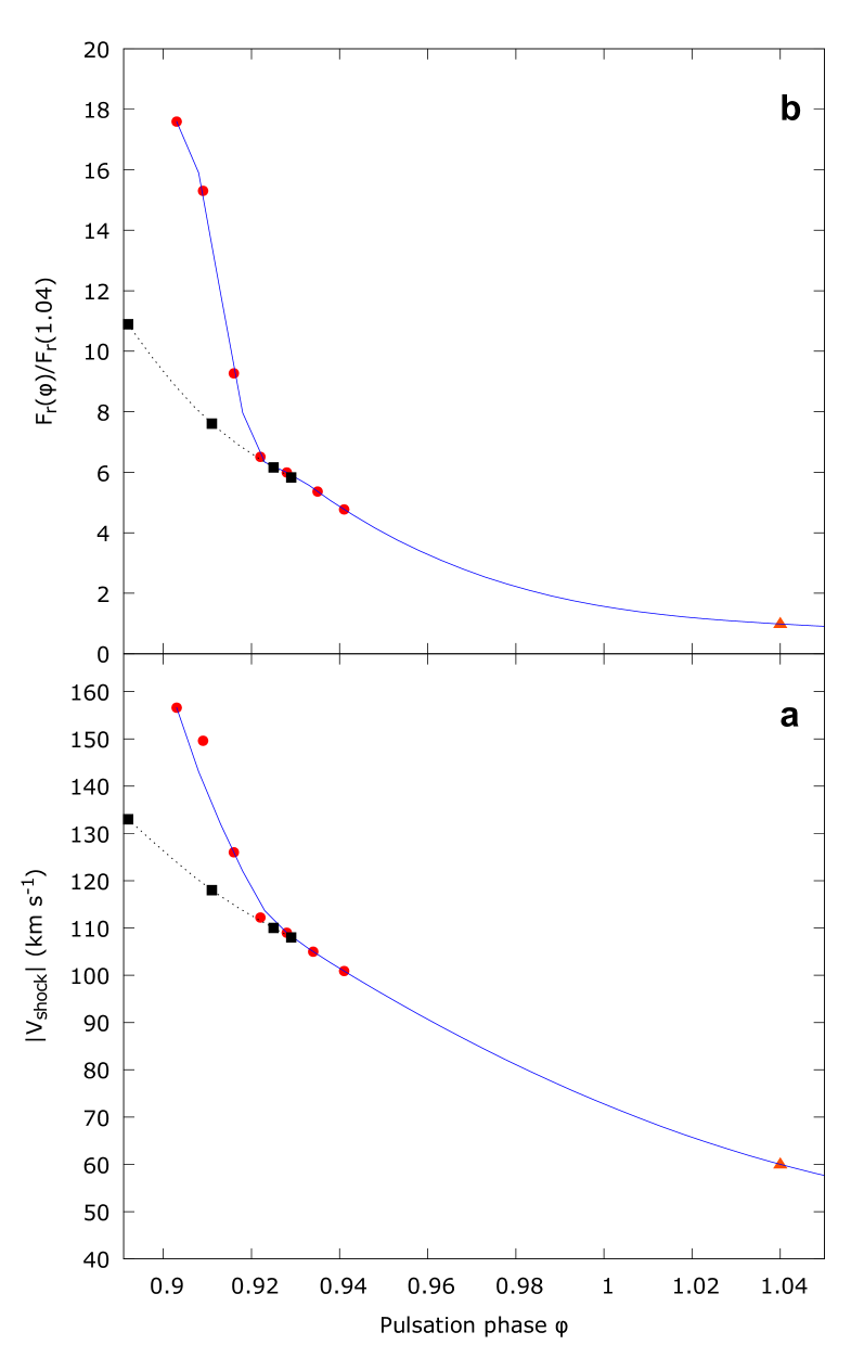
Figure 8: Phased kinetic and radiative flux measurements with trend curve.
Measurements points are the most probable values of $|V_{\textrm{shock}}|$ and $F_{r}(\varphi)/F_{r}(1.04)$. Associated uncertainties are computed in Tables 8 and 6. Red dots are measured values from 2014-Aug-13 while the red triangle represents the night of 2013-Oct-12. Velocities from April 2017 are black squares with the corresponding trend curve (grey dotted line).
Panel a: Evolution of $|V_{\textrm{shock}}|$ plotted with a cubic spline interpolation curve. In the phase interval $\varphi=0.90-0.92$, $V_{\textrm{shock}}$ decreases much more than in the phase interval $\varphi=0.92-1.04$. Thus, for 40% of the period, the shock front velocity decreases by a factor of more than three.
Panel b: Evolution of maximum values of $F_{r}(\varphi)/F_{r}(1.04)$ ratio plotted with a cubic spline interpolation curve. In the phase interval $\varphi=0.90-0.92$, the $F_{r}$ ratio decreases much more than in the phase interval $\varphi=0.92-1.04$. The flow of radiative losses increases rapidly with the speed of the shock front.

As discussed in Section 5.1, from our observations of the sodium and H$\alpha$ line profiles, it is not possible to distinguish independently the shock waves s1 and s2. We only observe the resulting shock s4+s3+s3’+s1+s2, called the main shock, obtained from the successive merging of s1, s2 and the secondary shocks s4, s3, and s3’. In their model RR41, Fokin & Gillet (1997) show the fusion of the two shocks s1 and s2. Moreover, they show that the amplitude of the shock s4+s3+s3’+s1 decreases rapidly first after merging s1 and again after merging s2 (see their Fig. 6). This weakening of the shock amplitude is consistent with our observations of the decreasing shock velocity when it rises in the atmosphere, as shown in Fig. 8. Thus, in the context of the physical and dynamic conditions taking place in the RR Lyr atmosphere, the shocks do not seem to present an accelerating phase above the photosphere.

6.3 Shock weakening regimes

During its propagation in the atmosphere, the shock is continuously decelerated (Fig. 8). It loses energy in two forms. One form is density dilution ($1/r^{2}$) as its radius $r$ increases. The other involves radiative losses as soon as it reaches a hypersonic speed, i.e., when its Mach number is greater than approximately 5. Using the Rankine-Hugoniot equation for energy and assuming that the shock is strong (until the isothermal limit), the maximum value of the radiative flux $F_{r}$ produced by the shock is (see Appendix)

$$F_{r}\leq\frac{1}{2}{\rho_{1}V_{\textrm{shock}}^{3}}\,,$$ (4)

where $\rho_{1}$ is the density of the unperturbed gas in front of the shock and $V_{\textrm{shock}}$ the shock front velocity. Thus, the flow of radiative losses increases rapidly with the shock front speed (to the third power). In the context of a realistic model, Fadeyev & Gillet (2001) estimated the irreversible loss occurring in the shock wave energy. Comparing the radiation flux emerging from the boundary of the shock layer with the total energy flux, they showed that the radiative losses increase very rapidly with increasing shock front velocity. They showed that 70% or more of the shock energy is lost in radiative form as soon as the shock front velocity is greater than 50  km s^-1 for physical conditions occurring in the atmosphere of pulsating stars with unperturbed gas of temperature between $T_{1}=3\,000$ K and $T_{1}=6\,000$ K with a density $\rho_{1}=10^{-10}$ g cm^-3.

Consequently, applying the equation above, the shock would lose, in first approximation, up to 18 times more radiation energy at $\varphi=0.903$, 15 times at $\varphi=0.909$, and only 6 times at $\varphi=0.928$ with respect to $\varphi=1.040$ (see Fig. 8b). Accordingly, the shock wave will probably lose most of its energy before the maximum brightness of the star. In 2017, when the maximum velocity of the shock was smaller (133 km s^-1 instead of 156 km s^-1), the radiative losses only represent 11 times those of the adiabatic regime. For the 2017 data we computed the radiative flux ratio with the 2014 value of $F_{r}(1.04)$, i.e., $V_{\mathrm{shock}}(1.04)$, assuming that $V_{\mathrm{shock}}$ converges asymptotically to the same value as 2014, as shown in Fig. 8.

In 2014, the deceleration is not uniform between the pulsation phases 0.90 and 1.04 (Fig. 8a). A two-step deceleration phase clearly appears. First, during a very short interval of the pulsation cycle (5% from $\varphi=0.90$ to $\varphi=0.95$), the shock velocity decreases by one-third of its value. This rate of fast decrease in the shock velocity occurs when the shock has a very large radiative loss, close to that of an isothermal shock. Then, up to $\varphi=1.04$, but slower, the shock velocity decreases by about a factor of $40\%$ over $10\%$ of the period. During this second phase, the radiative losses of the shock become secondary with respect to those induced by the geometric dilution due to the shock propagation. These two phases are clearly visible in Fig. 8.

In 2017, the maximum shock velocity did not reach a value (133 km s^-1) as large as in 2014 (156 km s^-1), i.e., a Mach number of 13 instead of 16. This difference seems sufficient to induce the transition between the two hydrodynamic regimes: the isothermal one, in which the radiative losses dominate, and the adiabatic one, in which the losses due to the geometric dilution are dominant.

Finally, when the intensity of the main shock wave is strong enough (isothermal phase), most of the shock wave energy is dissipated by radiative processes at the photospheric level, i.e., in the deep atmosphere. The remainder of the shock wave energy is dissipated by dilution in the high atmosphere when the radiative nature of the shock is no longer dominant (adiabatic phase).

6.4 Turbulent state of the atmosphere

Gillet et al. (1998) discussed the turbulence amplification in the atmosphere of a radially pulsating star, showing that it is due to the global compression of the atmosphere during the pulsation, and that it is also affected by strong shock waves propagating from the deep atmosphere. As already noticed by Kolenberg et al. (2010) and Fossati et al. (2014), among others, by definition the microturbulence velocity $V_{mic}$ characterizes a difference between observed and theoretical atmospheric parameters affecting the FWHM of an absorption spectral line:

$$V_{mic}\equiv\sqrt{FWHM^{2}_{obs}-FWHM^{2}_{model}}.$$ (5)

Therefore, it represents only the upper limit of atmospheric turbulence. Indeed, all line broadening effects such as velocity gradients or non-LTE effects are not always taken into account in atmosphere models.

A time variation in the microturbulence velocity $V_{mic}$ in the atmosphere of RR Lyrae has been estimated from a comparison of the observed and theoretical full width at half maximum (FWHM) curves of the Fe ii $4923.921$ Å absorption line by Fokin et al. (1999). This velocity $V_{mic}$ reflects motions on scales smaller than the line-forming region. Fokin et al. (1999) found that turbulence in this region varies from 2 to 7 km s^-1, over a large phase interval ($0.5\lesssim\varphi\lesssim 1.0$). The maximum (7 km s^-1) occurs at the pulsation phase $\varphi=0.7$ (during the light bump) and a secondary peak (3.5 km s^-1) occurs at $\varphi=0.2$. This prominent peak of $V_{mic}$ starts to appear when the two secondary shocks s4 and s3, as noted by Fokin & Gillet (1997), merge at $\varphi=0.52$ when $V_{mic}$ is at its lowest level (just after the phase of the maximum radius). The physical origin of the shock s4 is due to the accumulation of several weak compression waves at the sonic point during the beginning of the atmospheric compression, while s3 comes from the stop of the hydrogen recombination front near the phase of maximum expansion. In the case of RR Lyr, the peak maximum of the microturbulence velocity at 7 km s^-1 takes place when s4+s3 merge with the shock s3’ assumed to be caused by the 1H-mode (Fokin & Gillet, 1997). At this stage, the overall velocity of the shock s4+s3+s3’ is at a maximum, but still modest (55 km s^-1), although supersonic (Mach number $M\gtrsim 5$). Then the velocity of this shock slowly decreases almost to 40 km s^-1(Fokin & Gillet 1997, their Fig. 6). As a consequence the microturbulence velocity decreases until its rapid and abrupt rise induced this time by the arrival of the strong shocks s2 and s1 near $\varphi=0.91$, which have their origin in the $\kappa$-$\gamma$ mechanism associated with the H- and He-ionization zones. However, the effect of these two last shocks on the microturbulence velocity remains modest because they merge with s4+s3+s3’ in the upper part of the line-forming region of the Fe II line.

Recently, as part of an in-depth spectroscopic analysis of the Blazhko star RR Lyrae, Kolenberg et al. (2010) deduced a microturbulence velocity curve from the FWHM of the Fe ii line at $4508.288$ Å. In a complementary work, Fossati et al. (2014) showed this curve (green solid line in their Fig. 6); it presents an asymmetrical peak starting abruptly at $\varphi=0.9$, with a maximum near $\varphi=0.95$, and then a slow decrease until $\varphi=0.2$. It is centered just before the middle of the rising branch of the V-light curve. The minimum microturbulent velocity occurs at the maximum radius during the most stable pulsation phase, called the quiet phase, near $\varphi=0.33$. The value of the microturbulence velocity obtained by these authors is much higher (between 15 and 35 km s^-1) compared to the values between 2 and 7 km s^-1 found by Fokin et al. (1999). This may originate, at least in part, from the use of a static atmosphere model that is not able to take into account the strong velocity gradients present in the star. Indeed, such a velocity gradient is an important source of line broadening within a pulsating atmosphere (see Fokin et al. 1996). From the range of line formation depths covered by the measured lines, Fossati et al. (2014) estimate the $V_{mic}$ profiles in the corresponding optical depth range $\log\tau_{Ross}=-4$ to $\log\tau_{Ross}=0$, i.e., within the middle part of the atmosphere. The most striking fact is that the turbulent velocity continually decreases while the depth in the atmosphere increases. This is true for all pulsation phases—especially during the quiet phase and during the maximum compression induced by the global atmospheric pulsation—suggesting that the large-scale motions have no effect on the microturbulent velocity, , a disturbing result. Between the bottom and the top of the line-forming region, the microturbulence velocity varies from 3 to 20 km s^-1 except during the peak where the microturbulent velocity may be as high as 50 km s^-1, i.e., largely supersonic. In addition, Fossati et al. (2014) also point out that the microturbulence velocity of the deepest atmospheric layer increases, while that of the layer just above remains unchanged, also a surprising behavior.

As shown by Gillet et al. (1998), the turbulence amplification during a compression of the atmosphere without the presence of waves results from the variation of the density within the line-forming region. Because in radially pulsating stars, such as RR Lyrae stars, the atmospheric curvature is very small, it is possible to assume that the atmospheric distortion is not locally spherical but almost radial. Thus, compression must induce a preferential amplification direction. Gillet et al. (1998) estimated that the global atmospheric compression can be almost considered as an adiabatic homogeneous axial compression. Consequently, in the framework of a rapid distortion, the solenodial RDT model of Jacquin et al. (1993) appears to give the better quantitative prediction. As an application, for the radially pulsating star $\delta$ Cephei, the predicted turbulence amplification induced by the global atmospheric compression is consistent with the solenodial RDT (Gillet et al., 1998).

In the case of the presence of strong shocks as in the case of RR Lyrae stars, i.e., when the compression rate becomes higher than 2 (Mach number $\gtrsim 2$), radiative effects take place and adiabatic turbulence amplification theories break down. In this case, these theories give a considerable overestimation of the amplification (Gillet et al., 1998). Consequently, in the limiting case of very strong shocks (isothermal shocks), the compression ratio $\eta$ caused by the shock is $\eta\simeq\,M^{2}$. Basically, effects induced by radiative terms in conservation equations are certainly at the origin of the observed limit of the turbulence amplification. Nevertheless, the relevant theory does not yet exist and a new theoretical approach is required to take into account the radiative field within hypersonic shocks.

In this paper, we have established that the movements in the atmosphere are complex because the motion of atmospheric layers are not synchronous and are disturbed by the passage of strong shock waves. It is not possible to observe the steps of formation and acceleration of the main shock. Only its long deceleration phase is observable. During slightly less than 15% of the pulsation cycle ($0.90\leqq\varphi\leqq 1.04$), the main shock velocity decreases from 150 to 60 km s^-1, i.e., from a Mach number of 15 to 6. This strong deceleration occurs in only 2 hours, a rather short duration compared to the 13.6 h period. The radiative flux emitted by the shock then drops by a factor of 18 (Fig. 8.b), demonstrating that its energy is essentially dissipated in radiative form. All atmospheric layers do not reach their maximum expansion at the same time (a 2-hour difference between sodium and H$\alpha$ as shown in Fig. 7), generating rarefaction waves during the pulsation from $\varphi=0.30$ to $\varphi=0.50$ (see Table 5). Then a violent atmospheric compression occurs in the lower part of the atmosphere at $\varphi=0.36$ due to the rapid fall of the upper layers of the atmosphere.

Therefore, in the context of the extremely complex atmospheric pulsation of RR Lyr, it is not obvious to validate the use of successive static atmosphere models, assuming LTE and plane-parallel geometry, to interpret the different phenomena involved in this highly dynamic atmosphere. As a result, it seems difficult to get a good determination of the effective temperature through synthetic spectra fitting of the observed H$\gamma$ line, and of the surface gravity, which is obtained by imposing the ionization equilibrium for iron. Moreover, while imposing the equilibrium between the iron line abundance and equivalent widths to determine the microturbulent velocity, Fossati et al. (2014) introduced the need of a depth-dependent $V_{mic}$. Thus, in the context of a very disturbed atmosphere revealed by the observations reported in this article, it would be interesting to confirm the result of Fossati et al. (2014) regarding the depth-dependent of $V_{mic}$.

For $\delta$ Cephei, the maximum compression rate within the Fe II line-forming region induced by the global compression of the atmosphere near $\varphi=0.85$ is of the same order of magnitude as that caused by the main shock (Gillet et al., 1998). Because the maximum amplitude of the latter in RR Lyr is about 5 times larger than that of $\delta$ Cephei, we must expect that the dominant amplification phenomenon could be the main shock and not the global atmospheric compression. Moreover, as shown at the beginning of this section, the intensity of the main shock of RR Lyr is extremely large ($M\gtrsim 15$) only in the lowest part of the atmosphere because the shock velocity decreases very rapidly when it rises in the atmosphere, due to the intense radiative loss occurring in the shock wake. Consequently, the greatest microturbulence velocities should be observed essentially in the lower part of the atmosphere. Furthermore, as shown by Gillet et al. (1998), the presence of several secondary shocks in the atmosphere, as expected by pulsation models (Fokin & Gillet, 1997), can also be strong enough in the Fe II line-forming region to contribute to an amplification of the microturbulence velocity on the order of that induced by the global compression of the atmosphere. This is consistent with the result obtained by Fokin et al. (1999) because the wide maximum of microturbulence velocity spanning half a pulsation period occurs when secondary shocks s3 and s3’ are crossing the line-forming region. Also, the third H$\alpha$ emission observed near the pulsation phase 0.3 (Gillet et al., 2017) is interpreted as the consequence of a large atmospheric compression which provokes a strong and rapid increase of density and thus an appreciable amplification of the microturbulence velocity. This atmospheric compression could explain the secondary peak (3.5 km s^-1) of microturbulence velocity over the phase interval $0.10\leqq\varphi\leqq 0.35$.

Finally, in order to confirm that the microturbulence velocity increases with height in the atmosphere, as found by Fossati et al. (2014), it would be necessary to perform for RR Lyr a computation using a convective pulsation model including an extended atmosphere and allowing the generation of shock waves of large amplitude.

7 Conclusion

The objective of this paper was to determine from spectral observations the main dynamic phenomena occurring in the atmosphere of RR Lyr during a typical pulsation cycle. As the intensity of the pulsation cycles varies greatly over time, in particular because of the Blazhko effect, we considered a mean amplitude cycle, i.e., observations with a Blazhko phase close to $0.75$. The atmospheric phenomena that can occur during the cycles of extreme amplitude will be examined in a second paper.

This observational study was based on a series of 79 spectra sampled approximately every 15 min on the pulsation cycle. Thus, we are close to a temporal resolution of two hundredths (period $\sim$13 h 36 min). This resolution seems quite sufficient to follow all the developments occurring in spectral line profiles such as H$\alpha$ and Na D. Moreover, although the resolving power used is relatively modest ($R=11\,000$), all the potential spectral information that could exist in the profiles seems to be highlighted. All the spectra of this series were obtained between 7 and 18 April 2017; therefore, during the same Blazhko cycle. Observations were started at the Blazhko phase $\psi=0.75$ and were stopped at maximum Blazhko ($\psi=0.03$). Since the most intense hydrogen emission occurs at the beginning of the observation series, the intensity of the main shock corresponds to the average pulsation cycle ($\psi\sim 0.77$).

It should be noted that these observations were made with a modest telescope (35 cm). As RR Lyr is the brightest RR Lyrae star ($7<V<8$), an effective exposure time of 900 s allows a S/N of around 100 per pixel depending on weather conditions. As the feasibility conditions of this spectroscopic study were satisfying for this star, its extension to other RR Lyrae stars requires at least a one-meter class telescope.

The observed sodium and H$\alpha$ profiles presented in this paper did not allow us to resolve the shocks s1 and s2 individually. Only the main shock, the sum of these two shocks induced by the $\kappa$-mechanisms in the He and H-ionization subphotospheric layers, is confirmed. It is possible that observations with higher time resolution (exposure time less than 5 min), high signal-to-noise ratio ($S/N\gtrsim 100$) and high spectral resolution ($R\gtrsim 50\,000$) may allow the detection of these two shocks separately. Indeed, the observation of the shock s2, which is initiated deep below the photosphere, is probably impossible due to the excessive opacity of the gas. To observe s2, it would have to have existed above the photosphere before it merged with s1, but this does not seem to be the case from our observations.

One of the most striking results of this observational study is that we do not observe the acceleration phase of the main shock as soon as the H$\alpha$ emission produced in the shock wake becomes visible. Consequently, we directly observe the deceleration of the wave. The deceleration is faster when the shock is radiative than after when dilution phenomena become dominant. In the deep atmosphere (for 0.903¡$\varphi<0.941$), the shock is radiative when its Mach number is larger than 10, whereas when in the high atmosphere ($\varphi=1.040$) a Mach number around 6 is enough.

The sodium layer reaches its maximum expansion at $\varphi=0.320$, while for the layer in which the H$\alpha$ line core is formed, it is much later, at $\varphi=0.455$. Thus, a rarefaction wave appears in the atmosphere. This phenomenon is clearly predicted by the models of Fokin & Gillet (1997).

The so-called third H$\alpha$ emission is observed around $\varphi\sim 0.36$. It occurs when the ascending H$\alpha$ layer and the highest infalling atmospheric layers of the previous pulsating cycle compress the gas located between them. At this pulsation phase ($\varphi\sim 0.36$) the sodium layer, located in the deep atmosphere, already has an infalling movement, which means that the sodium does not participate in the compression inducing the third H$\alpha$ emission.

As previously shown by Gillet et al. (1998), the turbulence amplification of the atmospheric gas is mainly due to both the global compression of the atmosphere during its pulsation and to strong shock waves propagating through the atmosphere. In the case of RR Lyr, because amplitudes of shocks occurring within the atmosphere are large, the turbulence amplification is mostly caused by shocks, while that provoked by the global compression of the atmosphere seems secondary. This is the reason why the main peak of microturbulence velocity is very wide for RR Lyr conversely to the case of $\delta$ Cephei where it is quite narrow. Furthermore, because the main shock is always observed with a rapidly decreasing velocity during its propagation, the consecutive induced turbulence amplification should be highest in the lower part of the line-forming region of the Fe II line. It would be interesting to establish whether the microturbulence velocity increases or decreases with height in the atmosphere; this might be accomplished with a pulsation model including convection and an extended atmosphere and allowing the generation of shock waves of large amplitude.

In either case, in the future it would be constructive to know the variations in the shock intensity present in the atmosphere of RR Lyr, as well as those occurring in the various line profiles induced by atmospheric dynamics. However, this study requires a large observational survey because it is essential to integrate the effects due to the Blazhko phenomenon on atmospheric dynamics. This will be the goal of the second article in this series.

Finally, the data and work presented in this paper demonstrate further the increasing role of the amateur spectroscopy community in stellar surveys.

Appendix A The shock model of Fokin & Gillet (1997)

Fokin & Gillet (1997) computed more than 20 nonlinear, nonadiabatic, purely radiative pulsation models of the RR Lyrae  prototype, RR Lyr. However, since RR Lyr is located very close to the red edge of the instability strip, convection probably slightly affects the ionization zones of hydrogen and helium at the origin of the pulsation. These models go through the subphotospheric layers up to an extended atmosphere.

The shock waves are implicitly calculated with the Von Neumann-Richtmyer artificial viscosity that mimics the viscous dissipation of the kinetic energy of the shock. The consequence of this artificial viscosity is to widen the shock wake. Thus, it is not possible with this kind of numerical approach to resolve the fine structure of the shock because the spatial resolution is too weak (about $10^{3}$ km), or even to resolve the largest zone of the wake where photorecombinations occur (typically over a few km). As part of their numerical approach,  Fokin & Gillet (1997) note that the differentiation between a wave and a shock wave is not always obvious through the numerical model. They used the word “shock” when the density jump exceeds 5 over four consecutive mass zones.

The effect of excessive damping of the pulsation and waves due to the artificial viscosity have been tested by Fokin & Gillet (1997). It appears that their models are not very sensitive to the damping and cutoff parameters used. Consequently, the characteristics of the shocks and their associated hydrodynamics phenomena are stable and are present from one cycle to another.

During each pulsation cycle, four main shocks, with a well-identified physical origin, are produced in the outer part of the stellar envelope. In the case of RR Lyr, a fifth shock (shock s3’) is also highlighted; however, its physical origin has not yet been clearly identified. Contrary to the static regime, the extension of the atmosphere increases by several times during the pulsation. It is interesting to note that the four main shocks are stronger than in classical Cepheids, but their general features, especially their physical origin, are qualitatively similar.

The two strongest shocks are the consequence of the recombination of the ionization zones of hydrogen and helium in the subphotospheric region. Fokin & Gillet (1997) call theses shocks s1 and s2, respectively.

The scheme of phenomena predicted by Fokin & Gillet (1997) model are summarized in Table 9. Their models (including RR41) limit the description of the atmosphere to an external density to $10^{-14}$ g cm^-3. Thus, the maximum atmospheric height above the photosphere only reaches $0.22R_{ph}$ near the phase of the maximum expansion ($\varphi=0.55$).

Table 9: Scheme of phenomena from the Fokin & Gillet (1997) model (RR41) during a pulsation cycle.

$\varphi\ \mathrm{interval}$	Phenomenon
$0.75-0.80$	The $\kappa-\gamma$ mechanism associated with He-ionization and H-ionization zones provokes local overpressure, which transforms into outward progressive waves w1 and w2.
$0.80/0.93$	w1 and w2 rapidly become shocks s1 and s2, which emerge from the photosphere.
$0.96$	s1 merges with secondary shocks.
$1.01$	s2 merges with s1; apparition of the main shock.
$1.05$	The main shock leaves the described atmosphere.
$1.35$	Maximum expansion of the photosphere.
$1.60$	Maximum expansion of the highest atmospheric layers.

Appendix B Maximum radiative flux produced by the shock

This section describes which hypotheses are applied on the Rankine-Hugoniot equation system to obtain an upper limit on the radiation flux relation (Eq. 4) used in this paper.

Considering the total energy Rankine-Hugoniot relation, the radiation occurs through three different terms: the radiative pressure $p_{r}$, the specific radiative energy $e_{r}$, and the radiative flux $F_{r}$:

$$\frac{1}{2}u^{2}+e_{g}+e_{r}+\frac{p_{g}}{\rho}+\frac{p_{r}}{\rho}-\frac{F_{r}}{{\rho}{u}}={\rm constant}$$ (6)

In general, the exact value of the three radiative terms is difficult to determine, especially when the gas opacity is strongly frequency dependent. The first three angular moments of the specific intensity $I_{\mu\nu}$ of the radiation field are (Mihalas & Mihalas (1984), Sects. 6.4-6.6)

$$e_{r}\equiv\frac{1}{c}\int_{0}^{\infty}\,d\nu\int_{-1}^{+1}I_{\mu\nu}\,d\mu\qquad(\textrm{radiative energy}),$$ (7)

$$F_{r}\equiv\frac{1}{c}\int_{0}^{\infty}\,d\nu\int_{-1}^{+1}\mu\,I_{\mu\nu}\,d\mu\qquad(\textrm{radiative flux}),$$ (8)

and

$$p_{r}\equiv\frac{1}{c}\int_{0}^{\infty}\,d\nu\int_{-1}^{+1}\mu^{2}I_{\mu\nu}\,d\mu\qquad(\textrm{radiative pressure}),$$ (9)

where $\mu\equiv\cos\theta$ is the cosine of the polar angle $\theta$ between the direction of the considered radiation beam and the normal to the emitting surface. Nevertheless, when the fluid is close to the thermodynamical equilibrium, i.e., when it is optically thick, then the evaluation of the angular moments $I_{\mu\nu}$ is straightforward. In this case (see, e.g., Sampson (1965), Sect. 5.1 or Mihalas & Mihalas (1984) Sects. 6.8 and 6.9) the specific radiative energy is

$$e_{r}=e^{*}_{r}\equiv\frac{a_{r}T^{4}}{\rho}$$ (10)

and

$$p_{r}=p^{*}_{r}\equiv\frac{a_{r}T^{4}}{3}=\frac{\rho\,e^{*}_{r}}{3}\,,$$ (11)

where $a_{r}\equiv 4\sigma_{r}/c=7.56\,10^{-15}$ erg cm^-3 K^-4 is the radiation constant and $\sigma_{r}=5.67\,10^{-5}$ erg s^-1 cm^-2 K^-4 is the Stefan-Boltzmann constant. At the strictly thermodynamic equilibrium limit, the radiation field is isotropic. Consequently, since $F_{r}$ represents the flux, i.e., the sum of photon contributions in all directions, this means that the $F_{r}$ value is zero. Nevertheless, in the shock wake region located in front of the region where recombinations take place, the radiative flux cannot be in equilibrium because the gas is partially optically thin. This region includes the precursor, the shock front, and the first part of the wake where the thermalization occurs between heavy particles and electrons. In a first approximation, we can consider the wake recombination region as a blackbody at temperature $T$ and producing an equilibrium radiative flux,

$$F_{r}=F^{*}_{r}\equiv\sigma_{r}T^{4},$$ (12)

in the shock front direction. Because all atoms do not recombine at the same temperature and electronic density, $T$ must be considered as an effective temperature integrating large gradients of the physical variables present in the recombination region. Thus, from these thermodynamical equilibrium relations, we have

$$\frac{F^{*}_{r}/\rho\,u}{e^{*}_{r}}=\frac{1}{3}\frac{F^{*}_{r}/\rho\,u}{p^{*}_{r}/\rho}=\frac{c}{4u}\gg 1\,.$$ (13)

It should be noted that if the radiation field is larger in one direction (that of the outward flow), then $p_{r}$ will exceed its isotropic limit of $1/3e_{r}$ (see, e.g., Mihalas & Mihalas (1984) §66). In the extreme limit case occurring in plane waves, and more approximately in the outermost layers of the very extended atmosphere, we have $p_{r}=e_{r}$ (see Mihalas & Mihalas (1984) §66). Thus, in any case, $p_{r}$ remains close to $e_{r}$. Finally, at thermodynamical equilibrium, Eq. (13) shows that the radiative flux is always the main radiative contribution to the energy Rankine-Hugoniot relation.

This is explained by the fact that the speed of light is usually much higher than the relative post-shock velocity $u\equiv\,V_{\textrm{shock}}-{\textrm{v}}$. This is almost always the case in stellar atmospheres, where $u$ rarely exceeds 300 km s^-1 (0.1% of $c$). We note that for extremely fast shocks, such as supernovae explosions, where the initial shock front velocity is around 5% of the speed of light, the radiative pressure and energy are nearly equal to the gas pressure and energy. Thus, it is only for very fast flows of this kind that the three radiative terms must be considered.

Consequently, hereafter the only radiative term that we consider in the total energy Rankine-Hugoniot relation is the radiative flux $F_{r}$:

$$\frac{1}{2}u^{2}+e_{g}+\frac{p_{g}}{\rho}-\frac{F_{r}}{\rho u}={\rm constant}$$ (14)

The gas energy $e_{g}$ is the sum of the energy $e_{t}$ involved into the translational degrees of freedom of atoms and the energy $e_{i}$ stocked into their internal degrees of freedom (excitation, dissociation, ionization):

$$e_{g}=e_{t}+e_{i}\,.$$ (15)

In an ideal gas, the energy $e_{t}$ in translational degrees of freedom is given by

$$e_{t}=\frac{1}{\gamma-1}\frac{p}{\rho}\,,$$ (16)

where $\gamma$ is the ratio of specific heat.

If $E$, $D$, and $I$ respectively denote the excitation, dissociation, and ionization specific energies stored in the degrees of freedom of atoms, the internal gas energy $e_{i}$ is

$$e_{i}=E+D+I\,.$$ (17)

If indexes $1$ and $2$ denote the gas just before and just after the shock front, and if we neglect the gas energy in the unperturbed gas, then we have

$$\frac{1}{2}u_{1}^{2}-\frac{F_{r1}}{\rho_{1}\,u_{1}}=\frac{\gamma}{\gamma-1}\frac{p_{2}}{\rho_{2}}+e_{i2}.$$ (18)

If we consider the medium 2, the shock cools very quickly, and then we have $T_{2}=T_{1}$. In this case (isothermal shock), all the energy stored in the internal degrees of freedom of atoms is totally dissipated after the shock front. In addition, if the ballistic movement of the atmosphere has already been completed before the arrival of the next shock, then the velocity of the gas falling down on the star at the level of the shock is zero ($u_{1}=V_{\textrm{shock}}$). In these conditions, the above Rankine-Hugogniot relation reduces to

$$\frac{1}{2}V_{\textrm{shock}}^{2}=\frac{F_{r1}}{\rho_{1}\,V_{\textrm{shock}}}.$$ (19)

This means that the shock cannot radiate more radiative energy flux than

$$F_{r1}\leq\frac{1}{2}{\rho_{1}V_{\textrm{shock}}^{3}}\,.$$ (20)