Atoms trapped by a spin-dependent optical lattice potential:
realization of a ground state quantum rotor

Abstract

In a cold atom gas subject to a 2D spin-dependent optical lattice potential with hexagonal symmetry, trapped atoms execute circular motion around the potential minima. Such atoms are elementary quantum rotors. The theory of such quantum rotors is developed. Wave functions, energies, and degeneracies are determined for both bosonic and fermionic atoms, and magnetic dipole transitions between quantum rotor states are elucidated. Quantum rotors in optical lattices with precisely one atom per unit cell can be used as extremely high sensitivity rotation sensors, accelerometers, and magnetometers.

I Introduction

A quantum mechanical system in which the motion of a particle is constrained to a circular ring (or a multi-dimensional spherical shell) is an elementary quantum rotor (QR) Sachdev . References Sachdev ; wiki_Quantum-rotor state that “elementary QRs do not exist in nature”. Here we consider both bosonic and fermionic cold atoms subject to a 2D spin-dependent optical lattice potential (SDOLP) of hexagonal symmetry, and show that the trapped atoms behave as elementary QRs. We demonstrate that QRs with singly occupied sites (so deleterious spin relaxation effects are thereby suppressed) can be used as a high accuracy rotation sensor, accelerometer, and magnetometer.

Quantum rotors have been formed using Laguerre-Gaussian (LG) beams Allen_92 ; Clifford_98 , e.g., see Refs. Amico ; Kumar . However, these references mostly considered the many-body prosperities of cold atomic clouds in these beams and were not focused on elementary quantum rotors. In contrast, our interest is in singly occupied sites of SDOLPs so that interactions between QR atoms are suppressed. Hence the systems we consider are elementary QRs. Moreover, here we show that these QRs can be used as high accuracy rotation sensors, accelerometers, and magnetometers, and this not considered in Refs. Amico ; Kumar .

The outline of the paper is a follows. In Sec. II we present the model of the quantum rotors in the SDOLP. Section II.1 presents the 2D isotropic approximation for the SDOLP and Sec. II.2 discusses the exotic properties of these QRs. The stimulated Raman spectroscopy used to probe the QRs is considered in Sec. III, and in Sec. III.1 we focus on far-off-resonance Raman transitions between the ground state levels $n=0,\zeta=1/2$ and $n=0,\zeta=-1/2$. Section IV explains how to use the QRs in the SDOLP with singly occupied sites as a high precision magnetometer, Sec. V discusses the use of these QRs as rotation sensors and Sec. VI as accelerometers. In Sec. VII we provide estimates of the accuracy of measurements of rotation, acceleration and magnetic field using QRs, and in Sec. VIII we calculate the uncertainty due to shot noise in the Stokes and pump pulses. Finally, a summary and conclusion are presented in Sec. IX. In order to clarify some of the ideas presented in the main text, we provide a number of Appendices with background material and further details that substantiate the material presented in the main text. Specifically, Sec. A provides additional details regarding SDOLP, and Sec. B presents further details on the isotropic approximation for the potential near its minima. The QR areal probability density is studied in Sec. C. Section D provides a semiclassical description of the quantum QR. Finally, Sec. E discusses a method of distinguishing between the effects of rotation, acceleration and external magnetic field on the QR.

II The Model

Consider alkaline atoms trapped in the $x$-$y$ plane by a SDOLP Lin-Nature-2011 ; SOI-PRL-04 ; Galitski-Nature-2013 ; Juzeliunas-PRA-2010 ; Liu-PRL-2014 ; Zhang-PRL-2010 ; SOI-EuroPhysJ-13 . As shown schematically in Fig. 1, an optical lattice potential with hexagonal symmetry other-symmetry is formed by 6 coherent laser beams of wavelength $\lambda_{0}=\frac{2\pi}{q_{0}}$ and wave-vectors $\mathbf{q}_{n}=-q_{0}(\cos(n\pi/3),\sin(n\pi/3))$ with $n=1,2,3,\ldots,6$. The resultant electric field is $\mathbf{E}(\mathbf{r},t)=(\mathbf{E}({\bf r})e^{-i\omega_{0}t}+$ c.c.)/2 with amplitude $E_{0}$ and space dependent part

$$\mathbf{E}(\mathbf{r}) = E_{0}\sum_{n=1}^{6}\bm{\xi}_{n}e^{i\mathbf{q}_{n}\mathbf{r}},$$ (1)

where the polarization vectors ${\bm{\xi}}_{n}$ are

$$\bm{\xi}_{n}=\bigg{\{}\sqrt{1-\beta^{2}}~{}\mathbf{e}_{z}+\frac{\beta}{q_{0}}\mathbf{q}_{n}\times\mathbf{e}_{z}\bigg{\}}.$$ (2)

The electric field (1) is a linear combination of standing waves with in-plane and out-of-plane linear polarization with real mixing parameter $0<\beta<1$ (in what follows we take $\beta=1/\sqrt{2}$). It generates an effective SDOLP experienced by the atoms.

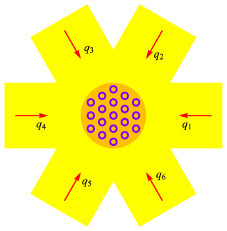
Figure 1: Laser beams (yellow) with wavevectors $\mathbf{q}_{n}$ in the $x$-$y$ plane generate an optical lattice potential with hexagonal symmetry. The orange disk in the center shows the physical region in which the optical lattice is located.

The quantum states of the trapped atoms are described by the electronic angular momentum $J$, the nuclear spin $I$, and the total internal atomic angular momentum quantum number $F$ (${\bf F}={\bf J}+{\bf I}$). As we shall see, atoms with $F\neq 0$ rotate in a closed circular ring in the $x$-$y$ plane around local minima of the scalar optical lattice potential. The corresponding orbital angular momentum operator is denoted by ${\bm{\ell}}$. The projections of ${\bf F}$, ${\bm{\ell}}$ and the total angular momentum of the QR, ${\bm{\mathcal{L}}}={\bf F}+{\bm{\ell}}$, on the $z$-axis are $f$, $m$ and $\zeta=f+m$ respectively. For bosonic (fermionic) atoms $\zeta$ is an integer (half-integer). Generically, the optical potential is not diagonal in $F$ nor in $f$ SOI-EuroPhysJ-13 , for further details see Appendix A. However, when the off-diagonal elements in $F$ are much smaller than the atomic hyperfine splitting, the mixing of atomic energy levels with different quantum numbers $F$ can be neglected.

For $J=1/2$, the optical lattice Stark interaction Hamiltonian is calculated as the second-order ac Stark shift. In the hyperfine basis it takes the form SOI-EuroPhysJ-13 ; hyperfine (see also Appendix A.2 for details),

$$H_{\mathrm{Stark}}(\mathbf{r})=V(\mathbf{r})1-\mathbf{B}(\mathbf{r})\cdot\mathbf{F},$$ (3)

where ${\bf 1}$ is the $(2F+1)$$\times$$(2F+1)$ unity matrix. The scalar optical potential $V(\mathbf{r})$ and fictitious magnetic field $\mathbf{B}(\mathbf{r})$ CCT (which has units of energy) are

$$V(\mathbf{r}) = -\frac{\alpha_{0}(\omega_{0})}{4}~{}\mathbf{E}^{*}(\mathbf{r})\cdot\mathbf{E}(\mathbf{r}),$$ (4a)

$$\mathbf{B}(\mathbf{r}) = \frac{i\alpha_{1}(\omega_{0})}{4(2I+1)}~{}[\mathbf{E}^{*}(\mathbf{r})\times\mathbf{E}(\mathbf{r})],$$ (4b)

where $\alpha_{0}(\omega_{0})$ and $\alpha_{1}(\omega_{0})$ are scalar and vector polarizabilities of the atom SOI-EuroPhysJ-13 ; Li-polarizability-2017 . For $J>1/2$, a tensor term is also present in Eq. (70) (see Ref. SOI-EuroPhysJ-13 ).

Both $V(\mathbf{r})$ and $\mathbf{B}(\mathbf{r})$ are periodic, $V(\mathbf{r})=V(\mathbf{r}+m_{1}\mathbf{a}_{1}+m_{2}\mathbf{a}_{2})$ and $\mathbf{B}(\mathbf{r})=\mathbf{B}(\mathbf{r}+m_{1}\mathbf{a}_{1}+m_{2}\mathbf{a}_{2})$, where $m_{1}$ and $m_{2}$ are integers, the lattice vectors are $\mathbf{a}_{j}=\lambda_{0}(\mathbf{e}_{x}\sin\theta_{j}+\mathbf{e}_{y}\cos\theta_{j})$, $j=1,2$, and $\theta_{j}=(-1)^{j}\pi/3$. $V(\mathbf{r})$ has minima at $\mathbf{r}_{\mathrm{min}}=m_{1}\mathbf{a}_{1}+m_{2}\mathbf{a}_{2}$. $\mathbf{B}(\mathbf{r})$ is a pseudovector SOI-EuroPhysJ-13 , and changes sign under time reversal (but the QR Hamiltonian is time reversal invariant). $V(\mathbf{r})$ and $\mathbf{B}(\mathbf{r})$ are plotted versus ${\bf r}$ in Fig. 7 in Appendix A.2.

The loss of atoms from the near-detuned SDOLP due to excited state spontaneous emission can be phenomenologically taken into account by including an imaginary contribution to the energy denominator of the second order ac Stark shift, see Eq. (62) of Appendix A. The loss rate is given by

$$\Gamma(\mathbf{r}) = \frac{V(\mathbf{r})\gamma_{\mathrm{e}}}{2\hbar\Delta}.$$ (5)

where $\Delta$ is the detuning of the optical frequency from resonance and $\gamma_{\mathrm{e}}$ is the inverse lifetime of the excited electronic state. As we shall soon see, the loss rate $\Gamma(\mathbf{r})$ will affect the accuracy of the sensors considered below.

Candidates for observing QR states include the fermions ²H, ⁶Li, ⁴⁰K, and the bosons ⁷Li, ²³Na, ³⁹K, ⁸⁵Rb and ⁸⁷Rb. All of these have nonvanishing $F$ in their ground electronic state hyperfine-H-He-PhysLett-2002 . Recoil temperatures $T_{0}={\mathcal{E}}_{0}/k_{B}$ for some of these fermionic and bosonic species are listed in Table 1.

Table 1: Recoil temperatures $T_{0}={\mathcal{E}}_{0}/k_{B}=\hbar^{2}q_{0}^{2}/(2Mk_{B})$ for some atoms.

. fermions bosons atom $T_{0}$ ($\mu$K) ${}^{2}{\text{H}}$ 321.7 ${}^{6}{\text{Li}}$ 3.536 ${}^{40}{\text{K}}$ 0.404 atom $T_{0}$ ($\mu$K) ${}^{7}{\text{Li}}$ 3.031 ${}^{23}{\text{Na}}$ 1.197 ${}^{39}{\text{K}}$ 0.414

II.1 2D Isotropic approximation

We assume hereafter that the depth of $V(\mathbf{r})$ at the minimum positions exceeds the recoil energy ${\mathcal{E}}_{0}=\hbar^{2}q_{0}^{2}/(2M)$, where $M$ is the atomic mass, and the low-energy atomic states are trapped and localized near these minima. For hexagonal symmetry, the scalar potential near the minimum at $\mathbf{r}=(0,0)$ is well-approximated by $V({\mathbf{r}})\approx\tilde{V}(r)$, where

$${\tilde{V}}(r)=-\frac{V_{0}}{6}~{}\Bigg{[}2+3J_{0}\bigg{(}\frac{2\pi r}{\lambda_{0}}\bigg{)}+J_{0}\bigg{(}\frac{2\sqrt{3}\pi r}{\lambda_{0}}\bigg{)}\Bigg{]},$$ (6)

and $V_{0}=\frac{9}{2}\alpha_{0}(\omega_{0})E_{0}^{2}$. The fictitious magnetic field near this minimum can be approximated by $\mathbf{B}(r)\approx\tilde{B}(r)\mathbf{e}_{r}$ where

$$\tilde{B}(r) = \frac{B_{0}}{3(2I+1)}~{}\Bigg{[}J_{1}\bigg{(}\frac{2\pi r}{\lambda_{0}}\bigg{)}+J_{1}\bigg{(}\frac{4\pi r}{\lambda_{0}}\bigg{)}+$$ (7)

$$\sqrt{3}~{}J_{1}\bigg{(}\frac{2\sqrt{3}\pi r}{\lambda_{0}}\bigg{)}\Bigg{]}.$$

Here $B_{0}=\frac{9}{2}\alpha_{1}(\omega_{0})E_{0}^{2}$, $J_{n}(\rho)$ is the Bessel function of order $n$, and the unit vector $\mathbf{e}_{r}\equiv\hat{\bf{r}}$. The dependence of $V_{0}$ and $B_{0}$ on the detuning of $\omega_{0}$ from resonance is discussed in Appendix A.2.

The (fictitious) Zeeman interaction ${\bf B}({\bf r})\cdot{\bf F}$ is proportional to $F_{r}={\bf F}\cdot\mathbf{e}_{r}$ [since ${\bf B}({\bf r})$ is radial] and does not commute with the operators $F_{z}$ or $\ell_{z}$ ($=-i\partial_{\phi}$), but commutes with ${\mathcal{L}}_{z}=F_{z}+\ell_{z}$. Hence, $f$ and $m$ are not individually good quantum numbers of the total Hamiltonian but $\zeta$, the eigenvalue of the operator ${\mathcal{L}}_{z}$, is. The wave functions $\Psi_{n,\zeta}(\mathbf{r})$ and energy levels $\epsilon_{n,\zeta}$ of the trapped atoms satisfy the Schrödinger equation band_structure ,

$$\bigg{[}-\frac{\hbar^{2}\nabla^{2}}{2M}+{\tilde{V}}(r)-\tilde{B}(r)F_{r}-\epsilon_{n,\zeta}\bigg{]}\Psi_{n,\zeta}(\mathbf{r})=0,$$ (8)

and the functions $\Psi_{n,\zeta}(\mathbf{r})$ can be expanded as follows:

$$\Psi_{n,\zeta}(\mathbf{r}) = \frac{1}{\sqrt{2\pi r}}\sum_{\sigma}\psi_{n,\zeta,\sigma}(r)e^{i\zeta\phi}\chi_{\sigma}(\phi).$$ (9)

Here $\chi_{\sigma}(\phi)$ are spinor eigenfunctions of $F_{r}$, i.e., $F_{r}\chi_{\sigma}(\phi)=\sigma\chi_{\sigma}(\phi)$, ($\sigma$ should not be confused with $f$, the eigenvalue of $F_{z}$).

Explicitly, for $F=1/2$ (e.g., ⁶Li), $\sigma=\pm 1/2$, and $\chi_{\sigma}(\phi)$ is given by

$$\chi_{\sigma=\pm 1/2}(\phi)=\frac{1}{\sqrt{2}}~{}\Big{\{}e^{-\frac{i\phi}{2}}\chi_{\uparrow}^{(z)}\pm e^{\frac{i\phi}{2}}\chi_{\downarrow}^{(z)}\Big{\}},$$

where $\chi_{f}^{(z)}$ are eigenfunctions of $F_{z}$ with eigenvalues $f$. Inserting the expansion (9) into Eq. (8) we obtain,

$$\bigg{[}-\frac{\hbar^{2}}{2M}\frac{\partial^{2}}{\partial r^{2}}+{\tilde{V}}(r)-\frac{1}{2}~{}{\tilde{B}}(r)+\zeta^{2}C(r)-\epsilon_{n,\zeta}\bigg{]}\times$$

$$\psi_{n,\zeta,1/2}(r)=\zeta C(r)\psi_{n,\zeta,-1/2}(r),$$ (10a)

$$\bigg{[}-\frac{\hbar^{2}}{2M}\frac{\partial^{2}}{\partial r^{2}}+{\tilde{V}}(r)+\frac{1}{2}~{}{\tilde{B}}(r)+\zeta^{2}C(r)-\epsilon_{n,\zeta}\bigg{]}\times$$

$$\psi_{n,\zeta,-1/2}(r)=\zeta C(r)\psi_{n,\zeta,1/2}(r),$$ (10b)

where the off-diagonal spin-flipped terms are proportional to $C(r)=\hbar^{2}/(2Mr^{2})$. The numerical calculations presented below will be for the fermionic case with $F=1/2$, assuming that $V_{0},|B_{0}|\gg{\mathcal{E}}_{0}$. The inequality $V_{0}\gg{\mathcal{E}}_{0}$ means that the potential wells are deep and the tunneling probability of the atoms between the wells is small. The wave functions and the eigen-energies $\epsilon_{n,\zeta}$ of the trapped atoms are computed by solving the Sturm-Liouville system of equations (10) with $V_{0}=100{\mathcal{E}}_{0}$, $B_{0}=180{\mathcal{E}}_{0}$. The resulting energies $\epsilon_{n,\zeta}$ are shown in Fig. 2. For the fermionic case, all the energy levels are two-fold degenerate, $\epsilon_{n,\zeta}=\epsilon_{n,-\zeta}$. The off-diagonal terms $\zeta C(r)\psi_{n,\zeta,\overline{\sigma}}(r)$ (where $\overline{\sigma}=-\sigma$) in (10) are a weak perturbation to the ground-state energy level, but not so for the excited states. The degenerate fermionic ground state has quantum numbers $(n,\zeta)=(0,\pm 1/2)$, and energy $\epsilon_{0,\pm 1/2}=-99.196\,{\mathcal{E}}_{0}$. The lowest energy excited states are orbital excitations with quantum numbers $(n,\zeta)=(0,\pm 3/2)$ and the radial excitations with quantum numbers $(1,\pm 1/2)$, see Fig. 2. The corresponding excitation energies are,

$$\epsilon_{0,\frac{3}{2}}-\epsilon_{0,\frac{1}{2}} = 6.011~{}{\mathcal{E}}_{0},$$ (11a)

$$\epsilon_{1,\frac{1}{2}}-\epsilon_{0,\frac{1}{2}} = 14.93~{}{\mathcal{E}}_{0},$$ (11b)

For temperatures $T\ll T_{\mathrm{orbit}}\equiv(\epsilon_{0,\frac{3}{2}}-\epsilon_{0,\frac{1}{2}})/k_{B}$, the trapped atoms are in their ground state. $T_{\mathrm{orbit}}$ is of order $T_{0}$, see Eq. (11a).

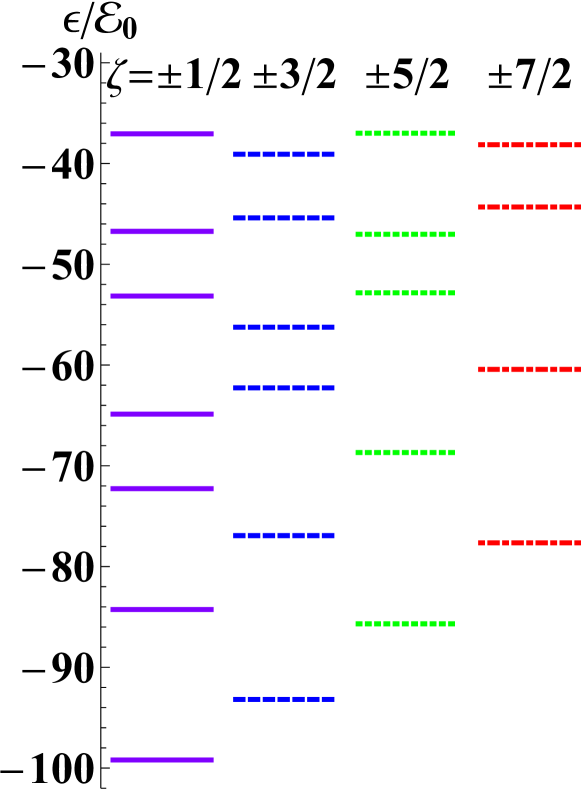
Figure 2: Fermionic QR energy levels for $F=1/2$ with $V_{0}=100\,{\mathcal{E}}_{0}$ and $B_{0}=180\,{\mathcal{E}}_{0}$. The solid purple, dashed blue, dotted green and dot-dashed red lines correspond to energy levels with $\zeta=\pm 1/2$, $\pm 3/2$, $\pm 5/2$, $\pm 7/2$. The energy levels with $n=0,1,\ldots$, go from bottom to top.

The ground state areal probability density,

$$\rho(r) = \big{|}\Psi_{0,1/2}({\bf r})\big{|}^{2},$$ (12)

depends only on $r$ and not on $\phi$ since the optical lattice potential is nearly isotropic about the potential minima. $\rho(r)$ has a maximum at $r=r_{0}=0.068\,\lambda_{0}$, and decays with $|r-r_{0}|$, as shown in Fig. 3. Thus, the atom is confined near a circular ring of radius $r_{0}$ (hence it is a QR Sachdev ). $\rho(r)$ vanishes linearly with $r$ as $r\to 0$. The QR ground state density can be observed as described in Ref. Bloch-position-Nature-2011 .

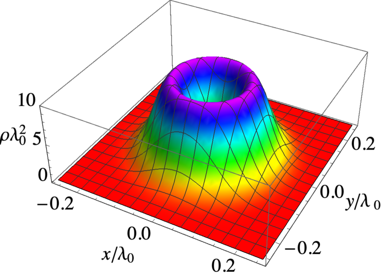
Figure 3: The ground state areal probability density (12) versus $\mathbf{r}=(x,y)$ for a $F=1/2$ fermionic atom.

II.2 Exotic properties of the QR state

The following exotic expectation values are obtained for the QR:

$$\big{\langle}n,\zeta\big{|}\ell_{z}\big{|}n,\zeta\big{\rangle} = \zeta-\big{\langle}n,\zeta\big{|}F_{z}\big{|}n,\zeta\big{\rangle},$$ (13)

$$\big{\langle}n,\zeta\big{|}\ell_{z}^{2}\big{|}n,\zeta\big{\rangle} = \zeta^{2}-\big{\langle}n,\zeta\big{|}2\zeta F_{z}-F_{z}^{2}\big{|}n,\zeta\big{\rangle}.$$ (14)

Recall that $\Psi_{n,\zeta}(\mathbf{r})=\langle{\bf r}|n,\zeta\rangle$ are eigenfunctions of ${\mathcal{L}}_{z}=\ell_{z}+F_{z}$ with eigenvalue $\zeta$, however $\Psi_{n,\zeta}(\mathbf{r})$ is not an eigenfunction of $F_{z}$ or $F_{z}^{2}$, and $\langle n,\zeta|F_{z}^{2}|n,\zeta\rangle\neq 0$.

For fermionic or bosonic QRs, the wave functions $\Psi_{n,\zeta}(\mathbf{r})$ in Eq. (9) are expressed as sums of products of spatial wave functions $\psi_{n,\zeta,\sigma}(r)e^{i\zeta\phi}$ and spin wave functions $\chi_{\sigma}(\phi)$. They have unusual symmetry relations under rotation through an angle $2\pi$ around the $z$ axis. The angular part of the spatial wave function, satisfies $e^{i\zeta(\phi+2\pi)}=\pm e^{i\zeta\phi}$ (upper sign for bosons and lower sign for fermions), and the spin wave function satisfies $e^{2\pi i{\mathcal{L}}_{z}}\chi_{\sigma}(\phi)=\chi_{\sigma}(\phi)$.

For bosonic QRs, $\zeta$ and $\sigma$ are integers, so the angular part of the spatial wave functions, $e^{i\zeta\phi}$, and the spin wave functions satisfy the properties, $e^{i\zeta(\phi+2\pi)}=e^{i\zeta\phi}$ and $e^{2\pi i{\mathcal{L}}_{z}}\chi_{\sigma}(\phi)=\chi_{\sigma}(\phi)$. The non-degenerate ground state $|n=0,\zeta=0\rangle$ is such that $\langle 0,0|F_{z}|0,0\rangle=0$, but $\langle 0,0|F^{2}_{z}|0,0\rangle\neq 0$, and therefore $\langle 0,0|\ell^{2}_{z}|0,0\rangle\neq 0$. The spin-excited QR states have $\zeta\neq 0$ and are doubly degenerate (see Eq. (1.23) in Ref. Sachdev ). All states have an areal density which vanishes at $r=0$.

For fermionic QRs, $\zeta$ and $\sigma$ are half-integer, and all states (including the ground state) are doubly degenerate. The ground state has $n=0$ and $\zeta=\pm 1/2$, and is an exotic QR since it is two-fold degenerate with finite orbital angular momentum. The expectation values of $\ell_{z}$ and $\ell_{z}^{2}$ are non-zero. For $F=1/2$, $\big{\langle}n,\zeta\big{|}\ell_{z}\big{|}n,\zeta\big{\rangle}=\frac{\zeta}{2}-\beta^{z}_{n,\zeta}$, and $\big{\langle}n,\zeta\big{|}\ell_{z}^{2}\big{|}n,\zeta\big{\rangle}=\frac{1}{2}-\big{|}\beta^{z}_{n,\zeta}\big{|}$, where

$$\beta_{n,\zeta}^{z}=\frac{1}{2}\sum_{\sigma}\int\psi_{n,\zeta,\sigma}\psi_{n,\zeta,-\sigma}dr.$$ (15)

A striking consequence of the above analysis, which will be substantiated below, is that ground state QRs with precisely one atom per site can serve as a rotation sensor, an accelerometer, and a magnetometer. For these applications and for the study of QRs in general, radio wave spectroscopy and Raman spectroscopy are valuable tools.

III QR Stimulated Raman Spectroscopy

Consider Raman transitions between the QR states $|n=0,\zeta=1/2\rangle$ and $|n=0,\zeta=-1/2\rangle$ that are split by an energy $\hbar\Delta_{QR}$ due to the presence of an external magnetic field, and/or rotation, and/or in-plane acceleration. We explicitly consider far-off-resonance radio wave transitions that are red-detuned from the $F=3/2$ atomic hyperfine state by a large detuning $\Delta_{\mathrm{hf}}$, $\Delta_{\mathrm{hf}}<0$ and $|\Delta_{\mathrm{hf}}|\gg\gamma_{\mathrm{hf}}$, where $\gamma_{\mathrm{hf}}$ is the decay rate of the $F=3/2$ hyperfine state (see Fig. 4 in Sec. III.1). Far-off-resonance stimulated Raman scattering can be treated as a two-level system with a generalized Raman Rabi frequency, $\Omega_{g}=\frac{\Omega_{p}\Omega_{s}}{\Delta_{\mathrm{hf}}}$. The pump laser has frequency $\omega_{p}$ and Rabi frequency $\Omega_{p}$, and takes the system up from the lower of the two QR states to a virtual intermediate state, and the Stokes radiation has frequency $\omega_{s}$ and Rabi frequency $\Omega_{s}$, and takes the system down from the virtual intermediate state to the upper of the two QR states. Let $\delta=\omega_{p}-\omega_{s}-\Delta_{QR}$ be the detuning from Raman resonance. The dressed-state Cohen-Tannoudji complex Hamiltonian in the 2-level $|n=0,\zeta=\pm 1/2\rangle$ manifold, which incorporates decay of the QR states, can be written as Sokolov_92

$$H_{\mathrm{Raman}}=\hbar\left(\begin{array}[]{cc}0-i\Gamma_{0,1/2}/2&\Omega_{g}/2\\ \Omega_{g}/2&\delta-i\Gamma_{0,-1/2}/2\end{array}\right).$$ (16)

Symmetry requires that the loss rates $\Gamma_{0,\pm 1/2}$ of the two QR states due to loss of atoms from the SDOLP be equal, $\Gamma_{0,1/2}=\Gamma_{0,-1/2}$; they are given by (see Sec. III.1 below for details):

$$\Gamma_{0,1/2} = \frac{\gamma_{\mathrm{e}}}{2\hbar\Delta}\sum_{\sigma}\bigg{\{}\int\tilde{V}(r)\psi_{0,1/2,\sigma}^{2}(r)dr$$ (17)

$$+\frac{{\mathrm{sign}}(\sigma)}{2}\int\tilde{B}(r)\psi_{0,1/2,\sigma}^{2}(r)dr\bigg{\}}.$$

Here $\Delta$ is the detuning of the laser beams generating the SDOLP and $\gamma_{\mathrm{e}}$ is the spontaneous emission decay rate of the ²P_3/2 excited state. The difference of the eigenvalues of $H_{\mathrm{Raman}}$, $\tilde{\Omega}=\sqrt{\delta^{2}+\Omega_{g}^{2}}$, is independent of $\Gamma_{0,1/2}$.

III.1 Far-Off-Resonance Raman Transitions Between $n=0,\zeta=1/2$ and $n=0,\zeta=-1/2$

Far-Off-Resonance Raman transitions between the QR states $|n=0,\zeta=1/2\rangle$ and $|n=0,\zeta=-1/2\rangle$ that are split by an energy $\hbar\Delta_{QR}$ is described by the model Hamiltonian (16). Here we derive Hamiltonian (16), its eigenvalues and eigenfunctions.

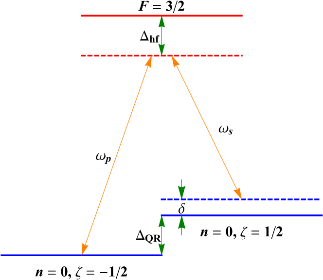
Figure 4: Schematic representation of the energy levels and photon energies for the far-off-resonance Raman transition between the split QR ground states.

Consider Raman transitions between the QR states $|n=0,\zeta=1/2\rangle$ and $|n=0,\zeta=-1/2\rangle$ that are split by an energy $\hbar\Delta_{QR}$ by the presence of a rotation, or an external magnetic field, or an in-plane acceleration. When the red detuning $\Delta_{\mathrm{hf}}$ from the $F=3/2$ hyperfine state is large enough, $|\Delta_{\mathrm{hf}}|\gg\gamma_{\mathrm{hf}}$ and $\Delta_{\mathrm{hf}}<0$, where $\gamma_{\mathrm{hf}}$ is the decay rate of the $F=3/2$ hyperfine state, see Fig. 4, the off-resonance intermediate $F=3/2$ state can be eliminated and the Raman process can be treated as a 2-level problem. The resultant generalized Raman Rabi frequency is given by $\Omega_{g}=\frac{\Omega_{p}\Omega_{s}}{\Delta_{\mathrm{hf}}}$. If we denote the energy difference between the two levels as $\hbar\Delta_{QR}$, the detuning from Raman resonance is $\delta=\omega_{p}-\omega_{s}-\Delta_{QR}$. The dressed-state 2-level non-Hermitian Hamiltonian Cohen-Tannoudji which incorporates decay of the QR states can be written as Sokolov_92

$$H_{\mathrm{Raman}}={\mathcal{H}}_{\mathrm{Raman}}-\frac{i\hbar}{2}~{}{\mathcal{G}},$$ (18)

where ${\mathcal{H}}_{\mathrm{Raman}}$ and ${\mathcal{G}}$ are 2$\times$2 Hermitian matrices; the Hermitian part ${\mathcal{H}}_{\mathrm{Raman}}$ in (18) is

$${\mathcal{H}}_{\mathrm{Raman}} = \hbar\left(\begin{array}[]{cc}0&\Omega_{g}/2\\ \Omega_{g}/2&\delta\end{array}\right).$$ (21)

It acts in the two dimensional Hilbert states spanned by $(1,0)^{T}=|0,1/2\rangle$ and $(0,1)^{T}=|0,-1/2\rangle$. The anti-Hermitian part originates from the decay rate in the optical lattice,

$$\Gamma(\mathbf{r}) = \frac{\gamma_{\mathrm{e}}}{2\hbar\Delta}~{}\Big{\{}\tilde{V}(r)+F_{r}\tilde{B}(r)\Big{\}},$$ (22)

where $\gamma_{\mathrm{e}}$ is the decay rate of the excited ²P_3/2 state, and $\Delta$ is the detuning of the laser frequency from the resonant frequency. When $|\Delta|\gg\gamma_{\mathrm{e}}$, we can apply perturbation theory and write the anti-Hermitian part the Hamiltonian (18) as

$${\mathcal{G}}_{\zeta,\zeta^{\prime}} = \int\Psi_{0,\zeta}^{{\dagger}}(\mathbf{r})\Gamma(\mathbf{r})\Psi_{0,\zeta^{\prime}}(\mathbf{r})~{}d^{2}\mathbf{r},$$

where $\Psi_{n,\zeta}(\mathbf{r})$ are the wave functions of the QR given by Eq. (10). Note that the atom in the quantum state with $\zeta=1/2$ or $-1/2$ orbits clockwise or counterclockwise around the minimum of the lattice potential. The decay rate (22) is isotropic. Therefore taking into account the symmetry of the wave function

$$\Psi_{n,-\zeta}(r,\phi)=F_{x}\Psi_{n,\zeta}(r,-\phi),$$

(which is true for $F=1/2$ atoms), we can write

$${\mathcal{G}}_{\zeta,\zeta^{\prime}}=\Gamma_{0,1/2}~{}\delta_{\zeta,\zeta^{\prime}},$$ (23)

where $\Gamma_{0,1/2}$ is given by Eq. (17). Eqs. (18), (21) and (23) yield Eq. (16).

Another source of uncertainty is spontaneous decay of the $F=3/2$ hyperfine state, which gives a decay rate

$$\Gamma_{\mathrm{hf}} = \frac{\gamma_{\mathrm{hf}}}{\hbar\Delta_{\mathrm{hf}}}~{}\sum_{\sigma}\int\bigg{\{}\tilde{V}(r)+\frac{{\mathrm{sign}}(\sigma)}{2}\tilde{B}(r)\bigg{\}}\times$$ (24)

$$\times\psi_{0,1/2,\sigma}^{2}(r)dr,$$

For ⁶Li atoms in the ground state, $\gamma_{\mathrm{hf}}=1.586\times 10^{-17}~{}{\text{s}}^{-1}$ Landau-Lifshitz-4 . Comparing Eqs. (17) and (24), one concludes that

$$\frac{\gamma_{\mathrm{hf}}}{\Delta_{\mathrm{hf}}}~{}\ll~{}\frac{\gamma_{\mathrm{e}}}{\Delta_{\mathrm{e}}},$$

hence $\Gamma_{\mathrm{hf}}\ll\Gamma_{0,1/2}$. Thus, in the following discussions we neglect $\Gamma_{\mathrm{hf}}$ since it is very small in comparison with $\Gamma_{0,1/2}$.

Eigenfunctions of the non-Hermitian Hamiltonian (16) are

$$\big{|}\psi_{+}\big{\rangle} = {\mathcal{U}}\big{|}0,1/2\big{\rangle}+{\mathcal{V}}\big{|}0,-1/2\big{\rangle},$$ (25a)

$$\big{|}\psi_{-}\big{\rangle} = {\mathcal{V}}\big{|}0,1/2\big{\rangle}-{\mathcal{U}}\big{|}0,-1/2\big{\rangle},$$ (25b)

where

$${\mathcal{U}}=\sqrt{\frac{\tilde{\Omega}+\delta}{2\tilde{\Omega}}},\ \ \ {\mathcal{V}}=\sqrt{\frac{\tilde{\Omega}-\delta}{2\tilde{\Omega}}},\ \ \ \tilde{\Omega}=\sqrt{\delta^{2}+\Omega_{g}^{2}}.$$

The corresponding eigenvalues are

$$\epsilon_{\pm}~{}=~{}\frac{\hbar\big{(}\delta-i\Gamma_{0,1/2}\big{)}}{2}\pm\frac{\hbar\tilde{\Omega}}{2}.$$

The difference $\epsilon_{+}-\epsilon_{-}=\hbar\tilde{\Omega}$ does not depend on $\Gamma_{0,1/2}$.

The time evolution of wave function of the QR with time, starting with the initial wave function $|0,1/2\rangle$ is specified by the time-dependent wave function

$$|\psi(t)\rangle = e^{-(\Gamma_{0,1/2}+i\delta)t/2}\times$$ (26)

$$\bigg{\{}\bigg{[}\cos\bigg{(}\frac{\tilde{\Omega}t}{2}\bigg{)}+\frac{i\delta}{\tilde{\Omega}}\sin\bigg{(}\frac{\tilde{\Omega}t}{2}\bigg{)}\bigg{]}\big{|}0,1/2\big{\rangle}-$$

$$\frac{i\Omega_{g}}{\tilde{\Omega}}\sin\bigg{(}\frac{\tilde{\Omega}t}{2}\bigg{)}~{}\big{|}0,-1/2\big{\rangle}\bigg{\}}.$$

The probabilities $P_{0,\pm 1/2}(t)$ to find the QR in the states $|0,\pm 1/2\rangle$ are given by $P_{0,\pm 1/2}(t)=\Big{|}\big{\langle}0,\pm 1/2\big{|}\psi(t)\big{\rangle}\Big{|}^{2}$. Using Eq. (26), we find

$$P_{0,1/2}(t) = \bigg{[}1-P_{0}\sin^{2}\bigg{(}\frac{\tilde{\Omega}t}{2}\bigg{)}\bigg{]}e^{-\Gamma_{0,1/2}t},$$ (27a)

$$P_{0,-1/2}(t) = P_{0}\sin^{2}\bigg{(}\frac{\tilde{\Omega}t}{2}\bigg{)}e^{-\Gamma_{0,1/2}t},$$ (27b)

where

$$P_{0}=\frac{\Omega_{g}^{2}}{\tilde{\Omega}^{2}}=\frac{\Omega_{g}^{2}}{\delta^{2}+\Omega_{g}^{2}}.$$

The Ramsey time-separated oscillating field method Ramsey_50 with Raman pulses Zanon using radio-frequency pump and Stokes radiation can be used to determine $\Delta_{QR}$, as we shall now show.

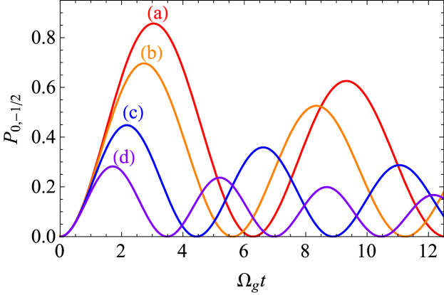
Figure 5: The probability $P_{0,-1/2}(t)$ in Eq. (27b) to find the QR in the state $|0,-1/2\rangle$ as a function of time for $\Gamma_{0,1/2}=0.05\,\Omega_{g}$, $\Omega_{g}=1$ and different values of $|\delta|$: (a) $\delta=0$, (b) $|\delta|=0.5\,\Omega_{g}$, (c) $|\delta|=\Omega_{g}$ and (d) $|\delta|=1.5\,\Omega_{g}$.

The probability $P_{0,-1/2}(t)$ is plotted in Fig. 5 for different values of $|\delta|$. The amplitude $P_{0}$ of $P_{0,-1/2}(t)$ is maximal when $\delta=0$. This is because $P_{0}$ is maximum when $\delta=0$ ($\Delta_{QR}=\omega_{p}-\omega_{s}$), and becomes very small for weak stimulated Raman scattering, i.e., when $|\delta|\gg\Omega_{g}$. Experimentally scanning $\omega_{s}$ and finding $\omega_{p}-\omega_{s}$ where $P_{0,-1/2}(t)$ is maximal yields $\Delta_{QR}$.

III.2 Ramsey Separated Oscillating Field Method

A preferable method of experimentally determining $\Delta_{QR}$ is to employ the Ramsey time-separated oscillating field method Ramsey_50 with Raman pulses Zanon . The QR initially in the ground state $|0,1/2\rangle$ is subjected to two sets of Raman pulses of duration $\tau_{p}$ separated by a delay time $T$, so the generalized Rabi frequency becomes time-dependent:

$$\Omega_{g}(t)=\left\{\begin{array}[]{ll}\Omega_{g}&\mbox{if $0\leq t\leq\tau_{p}$}\,,\\ 0&\mbox{if $\tau_{p}<t<T+\tau_{p}$}\,,\\ \Omega_{g}&\mbox{if $T+\tau_{p}\leq t\leq T+2\tau_{p}$}\,,\end{array}\right.$$ (28)

with $\Omega_{g}\tau_{p}\approx\pi/2$ and $T\gg\tau_{p}$. The effect of the first pulse is to evolve the initial state into a coherent superposition of the initial and final states. During the delay time between pulses, the system carries out phase oscillations. Finally, the second pulse rotates the state vector again by an angle of $\Omega_{g}\tau_{p}$. Fixing the delay time $T$ and measuring the population in the final state as a function of the detuning $\delta$ at the final time $T+2\tau_{p}$ yields a fringe pattern as shown in Fig. 6. The figure shows the Ramsey fringes obtained for a single QR and the value of $\Delta_{QR}$ such that $\delta=0$ is easy to identify from the fringe pattern.

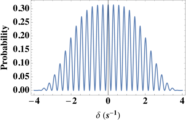
Figure 6: Ramsey fringes in the probability $P_{|0,-1/2\rangle}$ at the final time $T+2\tau_{p}$ plotted versus detuning $\delta$. The splitting $\Delta_{QR}$ is found by identifying where the detuning $\delta=\omega_{p}-\omega_{s}-\Delta_{QR}=0$.

IV Magnetometer

Atomic magnetometers often rely on a measurement of the Larmor precession of spin-polarized atoms in a magnetic field Budker_07 . One of the limitations on their sensitivity is spin relaxation. In our system, spin relaxation is highly suppressed if the lattice is singly occupied.

The degenerate ground state of a fermionic QR is split by the external field, and measuring the frequency splitting can accurately determine the external field. When the QR is placed in an external magnetic field, say $B_{\mathrm{ex}}\mathbf{e}_{z}$ (for simplicity), a Zeeman interaction term, $H_{B}=-g\mu_{B}B_{\mathrm{ex}}F_{z}$, must be included in the Schrödinger equation (8). The energy of the ground state calculated to first order in $B_{\mathrm{ex}}$ is

$$\epsilon_{0,\zeta}(B_{\mathrm{ex}}) = \epsilon_{0,\zeta}+\frac{2\zeta g\mu_{B}B_{\mathrm{ex}}}{2I+1}~{}\beta_{0,1/2}^{z}.$$ (29)

With $V_{0}=100\,{\mathcal{E}}_{0}$ and $B_{0}=180\,{\mathcal{E}}_{0}$, $\beta_{0,1/2}^{z}=0.1078$. Equation (29) shows that the external magnetic field splits the degeneracy of the energy levels with $\zeta=\pm 1/2$. The Raman scattering between these levels gives rise to Rabi oscillations with amplitude that has a maximum when $\omega_{p}-\omega_{s}=\Delta_{B}$, where

$$\Delta_{B} = \frac{{g\mu_{B}B_{\mathrm{ex}}}}{(2I+1)\hbar}~{}\beta_{0,1/2}^{z}.$$ (30)

The frequency splitting $\Delta_{B}$ can be experimentally measured, therefore the QR can be used as a magnetometer: measuring $\Delta_{B}$ and comparing with Eq. (30) yields the external magnetic field $B_{\mathrm{ex}}$. The uncertainty of $B_{\mathrm{ex}}$ results largely from the uncertainty of $\beta_{0,1/2}^{(z)}$ which is a function of the laser frequency $\omega$ and amplitude $E_{0}$. Hence, the accuracy of measuring $B_{\mathrm{ex}}$ is

$$\frac{\delta B_{\mathrm{ex}}}{B_{\mathrm{ex}}}=\frac{1}{\beta_{0,1/2}^{z}}~{}\sqrt{\big{(}\frac{\partial\beta_{0,1/2}^{z}}{\partial\omega}~{}\delta\omega\big{)}^{2}+\big{(}\frac{\partial\beta_{0,1/2}^{z}}{\partial E_{0}}~{}\delta E\big{)}^{2}},$$ (31)

where $\delta\omega$ and $\delta E$ are the uncertainties of $\omega$ and $E_{0}$. Additional analysis of $\delta B_{\mathrm{ex}}$, including the suppression of spin relaxation in a singly occupied optical lattice Viverit_04 ; Bloch_08 , directional external magnetic field effects, the lack of spectral line splitting due to the small anisotropy of the effective lattice potential, and measurement-time limitations, is provided in Sec. VII.

V Rotation Sensor

When the QR is in a non-inertial frame rotating with an angular velocity $\bm{\Omega}$ there is an additional term $H_{\Omega}=\hbar{\bm{\Omega}}\cdot{\bm{\mathcal{L}}}$ in the Hamiltonian, where ${\bm{\mathcal{L}}}=\mathbf{F}+\bm{\ell}$. For $\bm{\Omega}$ along the $z$-axis, the QR energy is,

$$\epsilon_{0,\zeta}(\Omega_{z}) = \epsilon_{0,\zeta}+\zeta\hbar\Omega_{z}.$$ (32)

In fact, for arbitrary $\bm{\Omega}$, Eq. (32) is valid to first order in $\bm{\Omega}$ (see Appendix E for details). The splitting of the ground state energy is $\Delta_{\Omega}=\Omega_{z}$, and the accuracy of measurement of the angular velocity due to spontaneous magnetic dipole transitions within the ground state QR manifold is $\delta\Omega_{z}=\delta\Delta_{\Omega}=4g^{2}\mu_{B}^{2}\Omega_{z}^{3}/(3\hbar c^{3})$. Additional analysis of $\delta\Omega_{z}$, including the suppression of spin relaxation in a singly occupied optical lattice Viverit_04 ; Bloch_08 , the lack of spectral line splitting due to the small anisotropy of the effective lattice potential, and measurement-time limitations, is given in Sec. VII.

VI Accelerometer

When the QR is in a non-inertial frame moving with a linear acceleration $\mathbf{a}$, an additional term $H_{a}=M{\bf a}\cdot{\bf r}$ must be included in the Hamiltonian. The energy of the ground state calculated to first order in $\mathbf{a}$ is

$$\epsilon_{0,\zeta}(a_{\parallel}) = \epsilon_{0,\zeta}+\zeta Ma_{\parallel}\varrho_{0,\zeta},$$ (33)

where $\varrho_{n,\zeta}=\int[\psi_{n,\zeta,1/2}^{2}(r)+\psi_{n,\zeta,-1/2}^{2}(r)]rdr$. The splitting of the ground state energy is $\Delta_{a}=Ma_{\parallel}\varrho_{0,\zeta}/\hbar$. The acceleration measurement accuracy $\delta a_{\parallel}$ is considered in Sec. VII.

VII Accuracy Estimates for ${\bf B}_{\mathrm{ex}}$, ${\bm{\Omega}}$, ${\bf a}$

$\delta{\bf B}_{\mathrm{ex}}$: The uncertainty of $B_{\mathrm{ex}}$ results largely from the uncertainty of the quantity $\beta_{0,1/2}^{z}$ which is a function of the laser frequency $\omega$ and amplitude $E_{0}$. Hence, the accuracy of measuring $B_{\mathrm{ex}}$ is given by Eq. (31). It is convenient to rewrite Eq. (31) as

$$\frac{\delta B_{\mathrm{ex}}}{B_{\mathrm{ex}}}=\frac{1}{\beta_{0,1/2}^{z}}~{}\sqrt{\big{(}\frac{\partial\beta_{0,1/2}^{z}}{\partial{\mathcal{E}}_{0}}~{}\delta{\mathcal{E}}\big{)}^{2}+\big{(}\frac{\partial\beta_{0,1/2}^{z}}{\partial{\mathcal{I}}_{0}}~{}\delta{\mathcal{I}}\big{)}^{2}},$$ (34)

where $\delta{\mathcal{E}}$ and $\delta{\mathcal{I}}$ are uncertainties of the recoil energy ${\mathcal{E}}_{0}$ and the laser intensity ${\mathcal{I}}_{0}$. $\beta_{0,1/2}^{z}$ depends on a single parameter, ${\mathcal{I}}_{0}/{\mathcal{E}}_{0}$, therefore

$${\mathcal{E}}_{0}~{}\frac{\partial\beta_{0,1/2}^{z}}{\partial{\mathcal{E}}_{0}}~{}=~{}-{\mathcal{I}}_{0}~{}\frac{\partial\beta_{0,1/2}^{z}}{\partial{\mathcal{I}}_{0}}.$$

Assuming that $\delta{\mathcal{I}}/{\mathcal{I}}_{0}\ll\delta\omega/\omega$, we get

$$\frac{\delta B_{\mathrm{ex}}}{B_{\mathrm{ex}}}=\frac{\delta{\mathcal{E}}}{\beta_{0,1/2}^{z}}~{}\bigg{|}\frac{\partial\beta_{0,1/2}^{z}}{\partial{\mathcal{E}}_{0}}\bigg{|}.$$

Numerical calculations for $V_{0}=100\,{\mathcal{E}}_{0}$ and $B_{0}=180\,{\mathcal{E}}_{0}$ give

$$\frac{\delta B_{\mathrm{ex}}}{B_{\mathrm{ex}}}~{}=~{}-\frac{0.075495~{}\delta\omega}{\omega},$$

where we have used the fact that $\delta{\mathcal{E}}/{\mathcal{E}}_{0}=2\,\delta\omega/\omega$. For lithium atoms, $\omega=2.808\times 10^{15}$ s^-1 Li-energy-PRA-1995 , and taking $\delta\omega=2\pi\times 160$ mHz $=1.005$ s^-1 mHz-laser-OptLett-2014 , we find

$$\frac{\delta B_{\mathrm{ex}}}{B_{\mathrm{ex}}} = 2.703\times 10^{-17}.$$ (35)

$\delta{\bm{\Omega}}_{\mathrm{z}}$: As already stated in Sec. V, the accuracy of measurement of the angular velocity due to spontaneous magnetic dipole transitions within the ground state QR manifold is $\delta\Omega_{z}=4g^{2}\mu_{B}^{2}\Omega_{z}^{3}/(3\hbar c^{3})$, hence

$$\frac{\delta\Omega_{z}}{\Omega_{z}^{3}}=1.614\times 10^{-44}~{}{\text{s}}^{2}.$$ (36)

For $\Omega_{z}=72.722~{}\mu$rad/s (the rotation frequency of Earth), $\delta\Omega_{z}=6.209\times 10^{-57}$ s^-1.

$\delta{\bf a}$: The acceleration measurement accuracy $\delta a_{\parallel}$ is given by

$$\frac{\delta a_{\parallel}}{a_{\parallel}}=\frac{1}{\varrho_{0,1/2}}~{}\sqrt{\Big{(}\frac{\partial\varrho_{0,1/2}}{\partial\omega}~{}\delta\omega\Big{)}^{2}+\Big{(}\frac{\partial\varrho_{0,1/2}}{\partial E_{0}}~{}\delta E\Big{)}^{2}}.$$ (37)

Taking into account the equalities,

$$\frac{\partial\varrho_{0,1/2}}{\partial\omega}~{}\delta\omega = \frac{\partial\varrho_{0,1/2}}{\partial{\mathcal{E}}_{0}}~{}\delta{\mathcal{E}},$$

$$\frac{\partial\varrho_{0,1/2}}{\partial E_{0}}~{}\delta E = \frac{\partial\varrho_{0,1/2}}{\partial{\mathcal{I}}_{0}}~{}\delta{\mathcal{I}},$$

where ${\mathcal{E}}_{0}$ is the recoil energy (88) and ${\mathcal{I}}_{0}\propto E_{0}^{2}$ is the intensity of the laser beam. Assuming that

$$\bigg{|}\frac{\partial\varrho_{0,1/2}}{\partial{\mathcal{I}}_{0}}\bigg{|}~{}\delta{\mathcal{I}}~{}\ll~{}\bigg{|}\frac{\partial\varrho_{0,1/2}}{\partial{\mathcal{E}}_{0}}\bigg{|}~{}\delta{\mathcal{E}},$$

we find that

$$\frac{\delta a_{\parallel}}{a_{\parallel}}\approx\frac{\delta{\mathcal{E}}}{\varrho_{0,1/2}}~{}\bigg{|}\frac{\partial\varrho_{0,1/2}}{\partial{\mathcal{E}}_{0}}\bigg{|}.$$

Numerical calculations for $V_{0}=100\,{\mathcal{E}}_{0}$ and $B_{0}=180\,{\mathcal{E}}_{0}$ give

$$\frac{1}{\varrho_{0,1/2}}~{}\bigg{|}\frac{\partial\varrho_{0,1/2}}{\partial{\mathcal{E}}_{0}}\bigg{|}=\frac{0.139986}{{\mathcal{E}}_{0}},$$

hence

$$\frac{\delta a_{\parallel}}{a_{\parallel}}=1.002\times 10^{-16}.$$

The measurement accuracy of an external magnetic field, angular velocity and linear acceleration are also affected by the energy-time uncertainty principle. Given a measurement time $T$, the measurement bandwidth is $1/(2T)$, and the accuracy of the QR magnetometer, accelerometer or gyroscope is proportional to $1/\sqrt{T}$ Budker-Kimball-book . For an optical lattice with $N$ QRs, the accuracies of the magnetometer, gyroscope and accelerometer are Budker-Kimball-book

$$\delta B_{u}=\frac{B_{\mathrm{ex}}}{\beta_{0,1/2}^{z}}~{}\bigg{|}\frac{\partial\beta_{0,1/2}^{z}}{\partial\omega}\bigg{|}~{}\sqrt{\frac{\delta\omega}{NT}},$$ (38)

$$\delta\Omega_{u}=\sqrt{\frac{\delta\Omega_{z}}{NT}},$$ (39)

$$\delta a_{u}=\frac{a_{\parallel}}{\varrho_{0,1/2}}~{}\bigg{|}\frac{\partial\varrho_{0,1/2}}{\partial\omega}~{}\bigg{|}~{}\sqrt{\frac{\delta\omega}{NT}}.$$ (40)

Here the subscript $u$ denotes uncertainty due to the finite measurement time, $\delta\omega$ is the uncertainty of the optical lattice laser frequency $\omega$, and $\delta\Omega_{z}$ is the angular velocity uncertainty given by Eq. (36). Taking $T=1$ s, and $N=4.99\times 10^{8}$ (which corresponds to an optical lattice of area 1 cm²), we get

$$\frac{\delta B_{u}}{B_{\mathrm{ex}}} = 1.74\times 10^{-20},$$ (41)

$$\frac{\delta\Omega_{u}}{\Omega_{z}^{3/2}} = 5.687\times 10^{-27}~{}{\text{s}}^{1/2},$$ (42)

$$\frac{\delta a_{u}}{a_{\parallel}} = 4.474\times 10^{-21}.$$ (43)

VIII Uncertainty due to Shot noise in the Stokes and pump pulses

Another source of uncertainty $\delta B_{\mathrm{ex}}$, $\delta\Omega$ and $\delta a$ arises from shot noise in the Stokes and pump pulses used to measure the detuning $\Delta_{\mathrm{QR}}$ of the QR using the Ramsey separated field method (see Figs. 4 and 6). Shot noise results in fluctuations in the position and amplitude of the population oscillations of the Ramsey fringes because the $\pi/2$ Raman pulses have Rabi frequencies which fluctuate $\Omega_{R}\tau$,

$$\phi_{R} \equiv \Omega_{R}\tau=\frac{\pi}{2}\pm\delta\phi_{R},$$

where

$$\delta\phi_{R}~{}\lesssim~{}\frac{\pi}{2}~{}\Bigg{(}\frac{1}{\sqrt{N_{p}}}+\frac{1}{\sqrt{N_{s}}}\Bigg{)},$$ (44)

and $N_{p}$ and $N_{s}$ are the number of photons of the pump and Stokes beams, assuming a Poissonian distribution of photon number. The uncertainty $\delta\Delta_{\mathrm{QR}}$ of $\Delta_{\mathrm{QR}}$ can be estimated from the variation of the probability for population transfer from the initial level of the split QR ground state level to the final level. A simple calculation shows that

$$\delta\Delta_{\mathrm{QR}}\lesssim\frac{\sqrt{1.5}\,\delta\phi_{R}}{\tau}\lesssim\frac{1.92}{\tau}~{}\Bigg{(}\frac{1}{\sqrt{N_{p}}}+\frac{1}{\sqrt{N_{s}}}\Bigg{)},$$ (45)

where we have used (44) for $\delta\phi_{R}$.

The ground-state hyperfine splitting of lithium atoms is $\omega_{\mathrm{hf}}=2\pi\times 228.2~{}{\text{MHz}}=1.434\times 10^{9}~{}{\text{s}}^{-1}$, so the energy of a Stokes and pump photons are $\hbar\omega_{s}\lesssim\hbar\omega_{p}\lesssim\hbar\omega_{\mathrm{hf}}$, where $\hbar\omega_{\mathrm{hf}}=1.51226\times 10^{-18}~{}{\text{erg}}$. The numbers of photons $N_{p}$ and $N_{s}$ can be estimated as

$$N_{\nu} = \frac{\pi r_{b}^{2}\tau I_{\nu}}{\hbar\omega_{\nu}},$$ (46)

where $I_{\nu}$ is the intensity of the pump ($\nu=p$) or Stokes ($\nu=s$) field, $r_{b}$ is the radius of the beam (which is assumed to be the same for the pump and Stokes beams) and $\tau$ is the pulse duration. Taking $I_{p}=5\times 10^{3}$ W/m², $I_{s}=2\times 10^{4}$ W/m², we get $\tau=1.644$ ms. For $r_{b}\approx 0.2$ m (the microwave wavelength), the numbers of photons (46) are

$$N_{p}\approx 7.467\times 10^{24},\ \ \ \ \ N_{s}\approx 2.987\times 10^{25},$$

so from Eq. (45) $\delta\Delta_{\mathrm{QR}}$ is

$$\delta\Delta_{\mathrm{QR}}~{}\approx~{}6.411\times 10^{-10}~{}{\text{s}}^{-1}~{}=~{}2\pi\times 0.102~{}{\text{nHz}}.$$

Knowing $\Delta_{\mathrm{QR}}$, the external magnetic field $B_{\mathrm{ex}}$, the angular velocity $\Omega$ or the acceleration $a$ of the non-inertial frame can be calculated using

$$B_{\mathrm{ex}} = \frac{(2I+1)\hbar\Delta_{\mathrm{QR}}}{g\mu_{B}\beta^{z}_{0,1/2}},$$ (47)

$$\Omega = \Delta_{\mathrm{QR}},$$ (48)

$$a = \frac{\hbar\Delta_{\mathrm{QR}}}{M\varrho_{0,1/2}}.$$ (49)

Here $I=1$ is the nuclear spin of ⁶Li atoms, $\beta_{0,1/2}^{z}=0.1078$, $M$ is the atomic mass and $\varrho_{0,1/2}=0.0987\lambda_{0}$, where $\lambda_{0}$ is the wavelength of the laser beam creating the optical lattice. For ⁶Li atoms, $\lambda_{0}=670.8$ nm, and therefore $\varrho_{0,1/2}=66.18$ nm.

When the optical lattice has $N$ quantum rotors, uncertainties of external magnetic field $B_{\mathrm{ex}}$, angular velocity $\Omega$ and acceleration $a$ due to the shot noise are given by,

$$\delta B_{\mathrm{ex}} = \frac{1}{\sqrt{N}}~{}\frac{(2I+1)\hbar~{}\delta\Delta_{\mathrm{QR}}}{g\mu_{B}\beta^{z}_{0,1/2}},$$ (50)

$$\delta\Omega = \frac{\delta\Delta_{\mathrm{QR}}}{\sqrt{N}},$$ (51)

$$\delta a = \frac{1}{\sqrt{N}}~{}\frac{\hbar~{}\delta\Delta_{\mathrm{QR}}}{M\varrho_{0,1/2}}.$$ (52)

For $N=4.99\times 10^{8}$ ⁶Li atoms,

$$\delta B_{\mathrm{ex}} = 4.54\times 10^{-24}~{}{\text{Tesla}},$$

$$\delta\Omega = 2.87\times 10^{-14}~{}{\text{s}}^{-1},$$

$$\delta a = 4.58\times 10^{-15}~{}{\text{m/s}}^{2}.$$

Compare this result with the uncertainties of the magnetic field and angular velocity of the Earth, and the acceleration due to gravity derived in Sec. VII,

$$\delta B_{u} = 7.8\times 10^{-25}~{}{\text{Tesla}},$$

$$\delta\Omega_{u} = 3.6\times 10^{-33}~{}{\text{s}}^{-1},$$

$$\delta a_{u} = 4.4\times 10^{-20}~{}{\text{m/s}}^{2}.$$

Hence the shot noise contribution to the uncertainty is larger than the uncertainty due to the decay rate of the excited hyperfine state.

IX Summary and Conclusions

The wave function of QRs, atoms trapped by a SDOLP, are confined to circular rings of radius $r_{0}$ with center at the minima of the scalar lattice potential. SDOLPs with precisely one atom per site (for which suppress spin-relaxation) can be used as ultra-high accuracy rotation sensors, accelerometers or magnetometers. The Ramsey time-separated oscillating field method with far-off-resonance Raman pulses between the split ground state of fermionic QRs can be used as a spectroscopic measurement technique for these applications, with a major accuracy limitation due to measurement-time uncertainty as outlined in Secs. VII and VIII. Bosonic QRs have ground states which are not degenerate, but their excited states are degenerate. The splitting of the excited states in the presence of rotation, in-plane acceleration or magnetic fields can also be used for sensing.

Appendix A Optical lattice potential

Consider a 2D hexagonal optical lattice potential produced by six coherent laser beams having a superposition of in-plane and out-of-plane linear polarization with a configuration shown in Fig. 1. Note that other configurations, e.g., three or four laser beams instead of six, can also produce a SDOLP, but we shall not consider other configurations here. The wavelength, wave number, and frequency of the laser beams are $\lambda_{0}$, $q_{0}=2\pi/\lambda_{0}$ and $\omega_{0}=q_{0}c$, where $c$ is the speed of light. The optical lattice frequency should be slightly detuned to the red of resonance. For ⁶Li atoms, the resonant wavelength is $\lambda_{\mathrm{res}}=670.98$ nm. The resultant electric field is given by $\mathbf{E}(\mathbf{r},t)=[\mathbf{E}(\mathbf{r})e^{-i\omega_{0}t}+{\mathrm{c.c.}}]/2$ where the spatial dependence of the field is

$$\mathbf{E}(\mathbf{r})=E_{0}\sum_{n=1}^{6}\bm{\xi}_{n}e^{i\mathbf{q}_{n}\mathbf{r}}.$$ (53)

The wavevectors $\mathbf{q}_{n}$ are

$$\mathbf{q}_{1}~{}=~{}-\mathbf{q}_{4}~{}=~{}-q_{0}~{}\mathbf{e}_{x},$$

$$\mathbf{q}_{2}~{}=~{}-\mathbf{q}_{5}~{}=~{}-\frac{q_{0}}{2}~{}\Big{\{}\mathbf{e}_{x}+\sqrt{3}~{}\mathbf{e}_{y}\Big{\}},$$ (54)

$$\mathbf{q}_{3}~{}=~{}-\mathbf{q}_{6}~{}=~{}\frac{q_{0}}{2}~{}\Big{\{}\mathbf{e}_{x}-\sqrt{3}~{}\mathbf{e}_{y}\Big{\}},$$

and the unit vectors $\mathbf{e}_{x}$, $\mathbf{e}_{y}$ and $\mathbf{e}_{z}$ are parallel to the $x$, $y$ and $z$ axes. The polarization vectors $\bm{\xi}_{n}$ ($1\leq n\leq 6$) are $\bm{\xi}_{n}=\Big{\{}\sqrt{1-\beta^{2}}~{}\mathbf{e}_{z}+\frac{\beta}{q_{0}}~{}\big{[}\mathbf{q}_{n}\times\mathbf{e}_{z}\big{]}\Big{\}}$, where $\beta$ is real and lies in the interval $0\,<\,\beta\,\leq\,1/\sqrt{2}$. Hereafter, we take $\beta=1/\sqrt{2}$.

For an arbitrary atom with electronic angular momentum ${\bf J}$, the electric field generates an effective SDOLP SOI-EuroPhysJ-13 ,

$$U(\mathbf{r}) = -\frac{1}{4}~{}\Bigg{\{}\alpha_{n,J}^{s}(\omega_{0})~{}\mathbf{E}^{*}(\mathbf{r})\cdot\mathbf{E}(\mathbf{r})-$$ (55)

$$-\frac{i\alpha_{n,J}^{v}(\omega_{0})}{2J}~{}\big{[}\mathbf{E}^{*}(\mathbf{r})\times\mathbf{E}(\mathbf{r})\big{]}\cdot{\mathbf{J}}+$$

$$+\frac{3\alpha_{n,J}^{t}(\omega_{0})}{2J(2J-1)}~{}\Big{[}\big{(}\mathbf{E}^{*}(\mathbf{r})\cdot{\mathbf{J}}\big{)}~{}\big{(}\mathbf{E}(\mathbf{r})\cdot{\mathbf{J}}\big{)}+$$

$$~{}~{}~{}+\big{(}\mathbf{E}(\mathbf{r})\cdot{\mathbf{J}}\big{)}~{}\big{(}\mathbf{E}^{*}(\mathbf{r})\cdot{\mathbf{J}}\big{)}-$$

$$~{}~{}~{}-\frac{2}{3}~{}J(J+1)~{}\mathbf{E}^{*}(\mathbf{r})\cdot\mathbf{E}(\mathbf{r})\Big{]}\Bigg{\}},$$

where $U$ is a $(2J+1)$$\times$$(2J+1)$ matrix in spin-space. Here $\alpha_{n,J}^{s}(\omega_{0})$, $\alpha_{n,J}^{v}(\omega_{0})$ and $\alpha_{n,J}^{t}(\omega_{0})$ are the conventional dynamical scalar, vector and tensor polarizabilities of the atom in the fine-structure level $|nJ\rangle$ with principal quantum number $n$ and total electronic angular momentum $J$ SOI-EuroPhysJ-13 :

$$\alpha_{n,J}^{s}(\omega_{0}) = \frac{\alpha_{n,J}^{(0)}(\omega_{0})}{\sqrt{3(2J+1)}},$$ (56)

$$\alpha_{n,J}^{v}(\omega_{0}) = -\frac{\sqrt{2J}~{}\alpha_{n,J}^{(1)}(\omega_{0})}{\sqrt{(J+1)(2J+1)}},$$ (57)

$$\alpha_{n,J}^{t}(\omega_{0}) = -\frac{\sqrt{2J(2J-1)}~{}\alpha_{n,J}^{(2)}(\omega_{0})}{\sqrt{3(J+1)(2J+1)(2J+3)}}.$$ (58)

The terms on the right hand side of Eq. (55) proportional to $\alpha_{J}^{s}(\omega_{0})$, $\alpha_{J}^{v}(\omega_{0})$ and $\alpha_{J}^{t}(\omega_{0})$ describe a spin-independent optical lattice potential, a Zeeman-type interaction and a tensor Stark-type interaction respectively. The scalar $\alpha_{n,J}^{(0)}(\omega_{0})$, vector $\alpha_{n,J}^{(1)}(\omega_{0})$ and tensor $\alpha_{n,J}^{(2)}(\omega_{0})$ polarizabilities of the atom in the fine-structure level $|nJ\rangle$ can be calculated as follows SOI-EuroPhysJ-13 :

$$\alpha_{n,J}^{(K)}(\omega_{0}) = \big{(}-1\big{)}^{K+J+1}\sqrt{2K+1}\sum_{n^{\prime},J^{\prime}}\big{(}-1\big{)}^{J^{\prime}}\times$$ (62)

$$\times\left\{\begin{array}[]{ccc}1&K&1\\ J&J^{\prime}&J\end{array}\right\}~{}\Big{|}\big{\langle}n^{\prime}J^{\prime}\big{\|}\mathbf{d}\big{\|}nJ\big{\rangle}\Big{|}^{2}\times$$

$$\times\frac{1}{\hbar}~{}{\mathrm{Re}}\bigg{(}\frac{1}{\omega_{n^{\prime},J^{\prime};n,J}-\omega_{0}-i\gamma_{n^{\prime},J^{\prime};n,J}/2}+$$

$$~{}~{}+\frac{(-1)^{K}}{\omega_{n^{\prime},J^{\prime};n,J}+\omega_{0}+i\gamma_{n^{\prime},J^{\prime};n,J}/2}\bigg{)}.$$

Here $K=0,1,2$ gives the scalar, vector and tensor polarizibilities, $\Big{\{}\begin{array}[]{ccc}1&K&1\\ J&J^{\prime}&J\end{array}\Big{\}}$ is the Wigner 6-$j$ symbol, and $\langle{nJ}\parallel\mathbf{d}\parallel{n^{\prime}J^{\prime}}\rangle$ is the reduced matrix elements of the dipole moment operator. The quantities $\omega_{n^{\prime},J^{\prime};n,J}=(\epsilon_{n^{\prime},J^{\prime}}-\epsilon_{n,J})/\hbar$ and $\gamma_{n^{\prime},J^{\prime};n,J}=\gamma_{n^{\prime},J^{\prime}}+\gamma_{n,J}$ are the angular frequency and linewidth of the transition between the fine-structure levels $|nJ\rangle$ and $|n^{\prime}J^{\prime}\rangle$.

A.1 Li atom scalar and vector polarizabilities

Equation (62) contains an expression for the scalar and vector polarizabilities of an atom in terms of matrix elements of the dipole operator between electronic wave functions. Here we use this expression in the special case of $J=1/2$ and compute the scalar and vector polarizabilities $\alpha_{s}(\omega)$ and $\alpha_{v}(\omega)$ of the Li atom in its ground-state whose electronic configuration (outside the closed 1s shell) is $2s~{}{}^{2}$S_1/2 Li-polarizability-2017 ,

$$\alpha_{0}(\omega) = -\frac{\alpha_{2,1/2}^{(0)}(\omega)}{\sqrt{6}},$$ (63a)

$$\alpha_{1}(\omega) = \frac{\alpha_{2,1/2}^{(1)}(\omega)}{\sqrt{3}},$$ (63b)

where $\alpha_{n,J}^{(K)}(\omega)$ ($K=0,1$) are the coupled polarizabilities given in Eq. (62), whereas the tensor polarizability $\alpha_{n,J}^{(K=2)}(\omega)=0$, see Ref. Li-polarizability-2017 for details. For the calculations of the reduced matrix elements $\langle n^{\prime}J^{\prime}||{\bf d}||nJ\rangle$ we need the electronic wave function of the Li atom in its ground and excited states. The ground state wave function with configuration $2s~{}{}^{2}$S_1/2 is

$$\Psi_{S,m_{s}}(r) = \frac{1}{\sqrt{4\pi}}~{}\psi_{2s}(r)\chi_{m_{s}},$$ (64)

where $\psi_{2s}(r)$ is the real valued radial wave function of the $2s$ electron and $\chi_{m_{s}}$ are spin wave functions, $m_{s}=\pm 1/2$. The radial and spin wave functions are normalized by the conditions, $\int\limits_{0}^{\infty}\psi_{2s}^{2}(r)r^{2}dr=1$, and $\chi_{m_{s}}^{{\dagger}}\chi_{m^{\prime}_{s}}=\delta_{m_{s},m^{\prime}_{s}}$.

The electronic wave functions of Li in the excited $2p~{}{}^{2}$P_1/2 and $2p~{}{}^{2}$P_3/2 states are given by

$$\Psi_{2p,J,m_{J}}(\mathbf{r}) = \psi_{2p}(r)\sum_{m_{L},m_{s}}C^{J,m_{J}}_{1,m_{L};1/2,m_{s}}\times$$ (65)

$$\times Y_{1,m_{L}}(\theta,\phi)\chi_{m_{s}}.$$

Here $\psi_{2p}(r)$ is the radial wave function of the $2p$ electron, $Y_{1,m_{L}}(\theta,\phi)$ are spherical harmonics with $m_{L}=0,\pm 1$, $\chi_{m_{s}}$ are spin wave functions with $m_{s}=\pm 1/2$, and

$$C^{J,m_{J}}_{1,m_{L};1/2,m_{s}}\equiv\Big{\langle}1m_{L}~{}\tfrac{1}{2}m_{s}\Big{|}Jm_{J}\Big{\rangle}$$

are Clebsch-Gordan coefficients. The radial wave functions and the spherical harmonics are normalized by the conditions, $\int\limits_{0}^{\infty}\psi_{2p}^{2}(r)r^{2}dr=1$, and

$$\int\limits_{0}^{2\pi}d\phi\int\limits_{0}^{\pi}\sin\theta d\theta~{}Y_{1,m_{L}}^{*}(\theta,\phi)Y_{1,m^{\prime}_{L}}(\theta,\phi)=\delta_{m_{L},m^{\prime}_{L}}.$$

The reduced matrix element of the electric dipole moment operator is,

$$d_{0}\equiv\Big{|}\big{\langle}eJ\big{\|}\mathbf{d}\big{\|}g1/2\big{\rangle}\Big{|}=e\int\limits_{0}^{\infty}\psi_{2s}(r)\psi_{2p}(r)r^{3}dr.$$ (66)

The 6-j symbols required in Eq. (62) for the Li atom are, $\Big{\{}\begin{array}[]{ccc}1&K&1\\ 1/2&J&1/2\end{array}\Big{\}}$, and are given by

$$\begin{array}[]{|c|c|c|}\hline\cr&J=1/2&J=3/2\\ \hline\cr K=0&1/\sqrt{6}&-1/\sqrt{6}\\ \hline\cr K=1&-1/3&-1/6\\ \hline\cr\end{array}.$$

We also need the resonant frequencies,

$$\omega_{J,1/2}=\frac{1}{\hbar}~{}\big{\{}\epsilon_{{\mathrm{p}},J}-\epsilon_{{\mathrm{s}},1/2}\big{\}},\ \ \ J=\frac{1}{2},~{}\frac{3}{2},$$

where $\epsilon_{{\mathrm{s}},1/2}$ is the energy of the ground ²S_1/2 state, and $\epsilon_{{\mathrm{p}},J}$ are the energies of the excited ²P_J states. The optical lattice frequency detuning from resonance should be smaller than the fine structure splitting (to have a significant effective magnetic field) but larger than the linewidth of the transitions. Hence, we assume that the frequency $\omega$ satisfies the inequalities,

$$\frac{\gamma_{1/2,1/2}}{2}~{}\ll~{}\omega_{1/2,1/2}-\omega~{}\ll~{}\omega_{3/2,1/2}-\omega_{1/2,1/2},$$

which imply

$$\frac{1}{\omega_{1/2,1/2}-\omega}~{}\gg~{}\frac{1}{\omega_{3/2,1/2}-\omega}~{}\gg~{}\frac{1}{\omega_{J,1/2}+\omega}.$$

The last inequality shows that the main contribution to the coupled polarizabilities (62) is from $(\omega_{J,1/2}-\omega)^{-1}$ (where $J=1/2,3/2$), whereas the terms $(\omega_{J,1/2}+\omega)^{-1}$ can be neglected. As a result, the coupled polarizabilities (62) are given by,

$$\alpha_{2,1/2}^{(0)}(\omega) = -\frac{d_{0}^{2}}{\sqrt{6}\hbar}~{}\frac{1}{\omega_{1/2,1/2}-\omega}-\frac{d_{0}^{2}}{\sqrt{6}\hbar}~{}\frac{1}{\omega_{3/2,1/2}-\omega},$$

$$\alpha_{2,1/2}^{(1)}(\omega) = \frac{d_{0}^{2}}{\sqrt{3}\hbar}~{}\frac{1}{\omega_{1/2,1/2}-\omega}-\frac{d_{0}^{2}}{2\sqrt{3}\hbar}~{}\frac{1}{\omega_{3/2,1/2}-\omega}.$$

The scalar and vector polarizabilities (63) are,

$$\alpha_{0}(\omega)=\frac{d_{0}^{2}}{6\hbar}~{}\frac{1}{\omega_{1/2,1/2}-\omega}+\frac{d_{0}^{2}}{6\hbar}~{}\frac{1}{\omega_{3/2,1/2}-\omega},$$ (68a)

$$\alpha_{1}(\omega)=\frac{d_{0}^{2}}{3\hbar}~{}\frac{1}{\omega_{1/2,1/2}-\omega}-\frac{d_{0}^{2}}{6\hbar}~{}\frac{1}{\omega_{3/2,1/2}-\omega}.$$ (68b)

The ratio of the vector and scalar polarizabilities is,

$$\frac{\alpha_{1}(\omega)}{\alpha_{0}(\omega)}=\frac{2\omega_{3/2,1/2}-\omega_{1/2,1/2}-\omega}{\omega_{3/2,1/2}+\omega_{1/2,1/2}-2\omega}\approx 2.$$ (69)

A.2 Spin-Dependent Optical Potential for $J=1/2$

The effective SDOLP $U({\bf r})$ in Eq. (55) acts in the Hilbert space of atomic states spanned by the basis kets $|nJFf\rangle$ where the quantum number $F$ corresponds to the total atomic angular momentum operator ${\bf F}={\bf J}+{\bf I}$ and $f$ is its projection on the $z$-axis SOI-EuroPhysJ-13 . Generically, $U({\bf{r}})$ is not diagonal in $F$ nor in $f$. However, when the off-diagonal elements with $F\neq F^{\prime}$ are much smaller than the hyperfine energy splitting of the atoms, we can neglect them. Within the subspace of fixed $n,J,F$ the matrix elements of $U({\bf r})$ are written as,

$$W_{f,f^{\prime}}(\mathbf{r}) = \big{\langle}nJFf\big{|}U(\mathbf{r})\big{|}nJFf^{\prime}\big{\rangle}.$$

As already stated, in the special case $J=1/2$, $\alpha_{n,J}^{(K=2)}(\omega_{0})=0$, i.e., the tensor Stark-type interaction operator vanishes. Hence, the optical lattice potential $W_{f,f^{\prime}}(\mathbf{r})$ takes the form SOI-EuroPhysJ-13 ,

$$W_{f,f^{\prime}}(\mathbf{r}) = V(\mathbf{r})\delta_{f,f^{\prime}}-\mathbf{B}(\mathbf{r})\cdot\mathbf{F}_{f,f^{\prime}},$$ (70)

where the scalar optical potential $V(\mathbf{r})$ and an fictitious magnetic field $\mathbf{B}(\mathbf{r})$ (which is taken to have units of energy) are given by Eq. (4). The scalar and vector dynamical polarizabilities of the atom are SOI-EuroPhysJ-13 ,

$$\alpha_{0}(\omega_{0}) = \frac{\alpha_{n,1/2}^{(0)}(\omega_{0})}{\sqrt{6}},$$ (71)

$$\alpha_{1}(\omega_{0}) = \big{(}-1\big{)}^{I+1/2+F}~{}\frac{\alpha_{n,1/2}^{(1)}(\omega_{0})}{\sqrt{3}},$$ (72)

Substituting Eq. (53) into Eq. (4a), and using polar coordinates $\mathbf{r}=(r,\phi)$, $x=r\cos\phi$, $y=r\sin\phi$, we obtain

$$V(\mathbf{r}) = -\frac{V_{0}}{3}-\frac{V_{0}}{6}\sum_{m=0}^{2}\cos\bigg{(}\frac{2\pi r}{\lambda_{0}}~{}\cos\big{(}\phi-m\theta_{0}\big{)}\bigg{)}-$$ (73)

$$-\frac{V_{0}}{18}\sum_{m=0}^{2}\cos\bigg{(}\frac{2\sqrt{3}\pi r}{\lambda_{0}}~{}\sin\big{(}\phi-m\theta_{0}\big{)}\bigg{)},$$

where $\theta_{0}=2\pi/3$. The potential strength $V_{0}$ is given by,

$$V_{0}=\frac{9\alpha_{0}(\omega_{0})}{2}~{}E_{0}^{2}.$$ (74)

Substituting Eq. (53) into Eq. (4b), we get

$$\mathbf{B}(\mathbf{r}) = B_{r}(\mathbf{r})\mathbf{e}_{r}+B_{\phi}(\mathbf{r})\mathbf{e}_{\phi}.$$ (75)

The components $B_{r}(\mathbf{r})$ and $B_{\phi}(\mathbf{r})$ of $\mathbf{B}(\mathbf{r})$ are expanded as,

$$B_{r}(\mathbf{r}) = \frac{B_{0}}{9(2I+1)}\sum_{m=0}^{3}\cos\big{(}\phi+m\theta_{0}\big{)}\times$$ (76a)

$$\times\sin\bigg{(}\frac{2\pi r}{\lambda_{0}}~{}\cos\big{(}\phi-m\theta_{0}\big{)}\bigg{)}+$$

$$+ \frac{B_{0}}{3\sqrt{3}(2I+1)}\sum_{m=0}^{2}\sin\big{(}\phi-m\theta_{0}\big{)}\times$$

$$\times\sin\bigg{(}\frac{2\sqrt{3}\pi r}{\lambda_{0}}~{}\sin\big{(}\phi-m\theta_{0}\big{)}\bigg{)}+$$

$$+ \frac{B_{0}}{9(2I+1)}\sum_{m=0}^{2}\cos\big{(}\phi-m\theta_{0}\big{)}\times$$

$$\times\sin\bigg{(}\frac{4\pi r}{\lambda_{0}}~{}\cos\big{(}\phi-m\theta_{0}\big{)}\bigg{)},$$

$$B_{\phi}(\mathbf{r}) = -\frac{B_{0}}{9(2I+1)}\sum_{m=0}^{3}\sin\big{(}\phi+m\theta_{0}\big{)}\times$$ (76b)

$$\times\sin\bigg{(}\frac{2\pi r}{\lambda_{0}}~{}\cos\big{(}\phi-m\theta_{0}\big{)}\bigg{)}+$$

$$+ \frac{B_{0}}{3\sqrt{3}(2I+1)}\sum_{m=0}^{2}\cos\big{(}\phi-m\theta_{0}\big{)}\times$$

$$\times\sin\bigg{(}\frac{2\sqrt{3}\pi r}{\lambda_{0}}~{}\sin\big{(}\phi-m\theta_{0}\big{)}\bigg{)}+$$

$$+ \frac{B_{0}}{9(2I+1)}\sum_{m=0}^{2}\sin\big{(}\phi-m\theta_{0}\big{)}\times$$

$$\times\sin\bigg{(}\frac{4\pi r}{\lambda_{0}}~{}\cos\big{(}\phi-m\theta_{0}\big{)}\bigg{)},$$

where the fictitious magnetic field strength $B_{0}$ is,

$$B_{0} = \frac{9\alpha_{1}(\omega_{0})}{2}~{}E_{0}^{2}.$$ (77)

The expansions (73) and (76) assure that $V(r,\phi)$, $B_{r}(r,\phi)$ and $B_{\phi}(r,\phi)$ are invariant under the transformation $\phi\to\phi^{\prime}=\phi-m\pi/3$, where $m$ is an integer. Thus, the optical lattice potential $V(\mathbf{r})$ and the fictitious magnetic field $\mathbf{B}(\mathbf{r})$ are invariant under rotations by $\pi/3$ radians around the $z$-axis (see Fig. 1),

$$V\bigg{(}U\Big{(}\frac{m\pi}{3}\Big{)}\mathbf{r}\bigg{)}=V(\mathbf{r}),$$

$$U\Big{(}\frac{m\pi}{3}\Big{)}\mathbf{B}\bigg{(}U\Big{(}\frac{m\pi}{3}\Big{)}\mathbf{r}\bigg{)}=\mathbf{B}(\mathbf{r}),$$ (78)

where the rotation matrix $U(\phi)$ is

$$U(\phi)=\left(\begin{array}[]{cc}\cos\phi&-\sin\phi\\ \sin\phi&\cos\phi\end{array}\right).$$

The optical potential (73) and the fictitious magnetic field (75) are shown in Fig. 7 and 7 for $\beta=1/\sqrt{2}$.

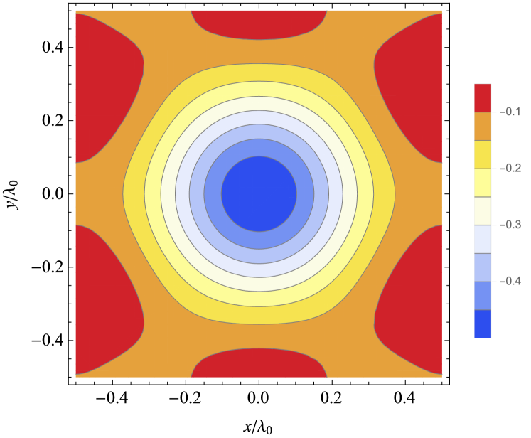
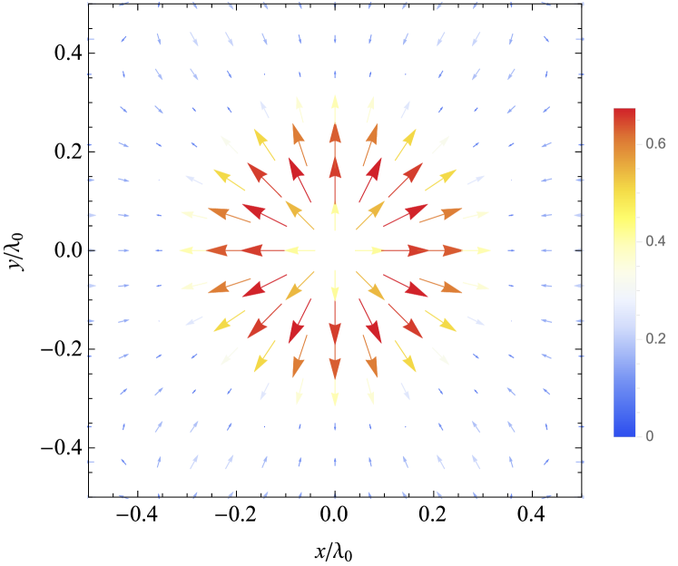
Figure 7: (a) The optical lattice potential $V(\mathbf{r})$, Eq. (73), and (b) the fictitious magnetic field (75) as functions of the Cartesian coordinates $x$ and $y$ for $\beta=1/\sqrt{2}$. The plot legends denote (a) $V(\mathbf{r})/V_{0}$ (contour plot with minimum indicated by deep blue). (b) $|\mathbf{B}(\mathbf{r})|/B_{0}$ (direction and strength indicated by arrows of varying length and color. $V_{0}$ and $B_{0}$ are given by Eqs. (74) and (77).

Appendix B Isotropic approximation for the spin-dependent optical lattice potential

The Fourier transform for $V(\mathbf{r})$, $B_{r}(\mathbf{r})$ and $B_{\phi}(\mathbf{r})$ are

$$V(r,\phi) = \sum_{m}\tilde{V}_{m}(r)e^{6im\phi},$$ (79)

$$B_{r}(r,\phi) = \sum_{m}\tilde{B}_{r,m}(r)e^{6im\phi},$$ (80)

$$B_{\phi}(r,\phi) = \sum_{m}\tilde{B}_{\phi,m}(r)e^{6im\phi},$$ (81)

where $m$ is an integer, and

$$\tilde{\mathcal{F}}_{m}(r)=\frac{1}{2\pi}\int\limits_{0}^{2\pi}{\mathcal{F}}(r,\phi)e^{-6im\phi}d\phi,\qquad{\mathcal{F}}=V,B_{r},B_{\phi}.$$

$V(r,\phi)$, $B_{r}(r,\phi)$ and $B_{\phi}(r,\phi)$ are real, and therefore

$$\tilde{\mathcal{F}}_{-m}(r) = \tilde{\mathcal{F}}_{m}^{*}(r).$$

Moreover, $V(r,\phi)$ and $B_{r}(r,\phi)$ are even with respect to the inversion $\phi\to-\phi$, and $B_{\phi}(r,\phi)$ is odd,

$$V(r,-\phi) = V(r,\phi),$$

$$B_{r}(r,-\phi) = B_{r}(r,\phi),$$

$$B_{\phi}(r,-\phi) = -B_{\phi}(r,\phi).$$

Therefore the Fourier components $\tilde{V}_{m}$, $\tilde{B}_{r,m}$ and $\tilde{B}_{\phi,m}$ satisfy the properties,

$$\tilde{V}_{m}(r) = \tilde{V}_{-m}(r),$$

$$\tilde{B}_{r,m}(r) = \tilde{B}_{r,-m}(r),$$

$$\tilde{B}_{\phi,m}(r) = -\tilde{B}_{\phi,-m}(r).$$

B.1 Isotropic approximation for $V(\mathbf{r})$

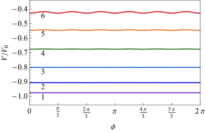
Figure 8: $V(\mathbf{r})$ (73) as a function of the polar angle $\phi$ for $\beta=\frac{1}{\sqrt{2}}$. The purple (1), blue (2), sky blue (3), green (4), orange (5) and red (6) curves denote $r=0.05\lambda_{0}$, $0.1\lambda_{0}$, $0.15\lambda_{0}$, $0.2\lambda_{0}$, $0.25\lambda_{0}$ and $0.3\lambda_{0}$.

Fig. 8 shows $V(\mathbf{r})$ as a function of $\phi$ for $\beta=1/\sqrt{2}$ and a few values of $r$. It is clear that for $r<0.3\lambda_{0}$, the potential is almost isotropic. Hence, for $r\lesssim 0.3\,\lambda_{0}$, the optical potential (73) can be well approximated by the isotropic potential $\tilde{V}(r)\equiv\tilde{V}_{0}(r)$ given by Eq. (6).

The lowest-order anisotropic correction to the potential in Eq. (79) is given in terms of the Fourier coefficients,

$$\tilde{V}_{1}(r)=\tilde{V}_{-1}(r)\approx\frac{V_{0}}{180}~{}\bigg{(}\frac{\pi r}{\lambda_{0}}\bigg{)}^{6}.$$ (82)

For $r=r_{0}=0.068\,\lambda_{0}$, where $r_{0}$ is radius where the areal probability density is maximal, $|\tilde{V}_{1}(r_{0})|\approx 5.281\times 10^{-7}\,V_{0}$, i.e., it is really small, and therefore the anisotropic corrections can be neglected for the ground and lowest energy eigenstates.

The isotropic potential $\tilde{V}_{0}(r)$ is shown in Fig. 10 (blue curve). Clearly, $\tilde{V}_{0}(r)$ is attractive and increases monotonically with $r$.

B.2 Isotropic approximation for $\mathbf{B}(\mathbf{r})$

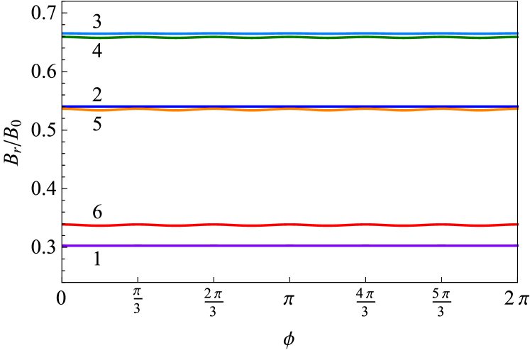
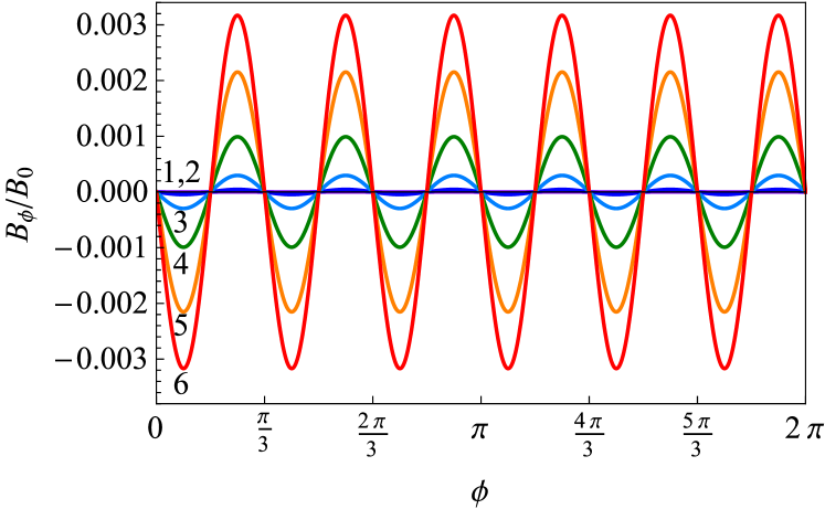
Figure 9: (a) $B_{r}(\mathbf{r})$ and (b) $B_{\phi}(\mathbf{r})$, Eq. (76), as functions of the polar angle $\phi$ for $\beta=\frac{1}{\sqrt{2}}$. The purple (1), blue (2), sky blue (3), green (4), orange (5) and red (6) curves denote $r=0.05\lambda_{0}$, $0.1\lambda_{0}$, $0.15\lambda_{0}$, $0.2\lambda_{0}$, $0.25\lambda_{0}$ and $0.3\lambda_{0}$.

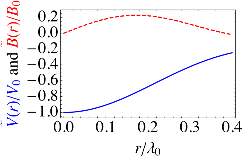
Figure 10: Spherically symmetric potential $\tilde{V}(r)\equiv\tilde{V}_{0}(r)$ in units of $V_{0}$ and the effective radial magnetic field $\tilde{B}(r)\equiv\tilde{B}_{r,0}(r)$ in units of $B_{0}$.

Figure 9 shows $B_{r}(\mathbf{r})$ and $B_{\phi}(\mathbf{r})$, Eq. (76), as functions of $\phi$ for $\beta=1/\sqrt{2}$ and several values of $r$. Clearly, for $r<0.3\lambda_{0}$, $B_{r}(\mathbf{r})$ depends on on $r$, whereas $B_{\phi}(\mathbf{r})$ oscillates quickly with $\phi$, but with very small amplitude. Hence, for $r\lesssim 0.3\lambda_{0}$, $B_{r}(\mathbf{r})$ can be approximated by the isotropic function $\tilde{B}(r)\equiv\tilde{B}_{r,0}(r)$

$$\tilde{B}_{r,0}(r) = \frac{B_{0}}{3(2I+1)}\Bigg{\{}J_{1}\bigg{(}\frac{2\pi r}{\lambda_{0}}\bigg{)}+J_{1}\bigg{(}\frac{4\pi r}{\lambda_{0}}\bigg{)}+$$ (83)

$$+\sqrt{3}~{}J_{1}\bigg{(}\frac{2\sqrt{3}\pi r}{\lambda_{0}}\bigg{)}\Bigg{\}},$$

and the isotropic part of $\tilde{B}_{\phi,0}(r)$ vanishes,

$$\tilde{B}_{\phi,0}(r)=0.$$

The lowest-order anisotropic corrections to $B_{r}(\mathbf{r})$ and $B_{\phi}(\mathbf{r})$ in Eqs. (80)-(81) are given by the Fourier coefficients

$$\tilde{B}_{r,1}(r)=\tilde{B}_{r,-1}(r)\approx-\frac{B_{0}}{120(2I+1)}~{}\bigg{(}\frac{\pi r}{\lambda_{0}}\bigg{)}^{5},$$ (84)

$$\tilde{B}_{\phi,1}(r)=\tilde{B}_{\phi,-1}^{*}(r)\approx-\frac{iB_{0}}{120(2I+1)}~{}\bigg{(}\frac{\pi r}{\lambda_{0}}\bigg{)}^{5}.$$ (85)

When $r=r_{0}=0.068\,\lambda_{0}$, $\big{|}\tilde{B}_{r,1}\big{(}r_{0}\big{)}\big{|}=\big{|}\tilde{B}_{\phi,1}\big{(}r_{0}\big{)}\big{|}\approx 1.236\times 10^{-6}~{}B_{0}$, is very small, and the anisotropic part of the magnetic field can be neglected for the ground and lowest excited energy eigenstates.

The isotropic effective radial magnetic field $\tilde{B}(r)$ is shown in Fig. 10 (red curve). Note that $\tilde{B}(0)=0$. There is a distance $r_{B}=0.1722\,\lambda_{0}$ such that for $r<r_{B}$, $\tilde{B}(r)$ increases with increasing $r$. $\tilde{B}(r)$ reaches its maximum, $\tilde{B}(r_{B})=0.6780\,B_{0}$, at $r=r_{B}$, and decreases for $r>r_{B}$. When $r=r_{c}=0.3827\,\lambda_{0}$, $\tilde{B}(r_{c})=0$, and for $r>r_{c}$, the fictitious magnetic field reverses its direction from $\hat{\mathbf{r}}$ to $-\hat{\mathbf{r}}$.

Appendix C Probability density for $F=1/2$

At finite temperature $T$, the probability density to find the atom at position ${\bf r}$ in the 2D plane is

$$\rho(r)=\frac{1}{Z}\sum_{n,\zeta}\big{|}\Psi_{n,\zeta}(\mathbf{r})\big{|}^{2}~{}e^{-\beta\epsilon_{n,\zeta}},$$

where

$$Z=\sum_{n,\zeta}e^{-\beta\epsilon_{n,\zeta}},$$

and $\beta=(k_{B}T)^{-1}$ is proportional to the inverse temperature. At low temperature, where $k_{B}T$ is much smaller than the orbital excitation energy [see Eq. (11a)], $\rho(r)$ is well approximated by Eq. (12). In the isotropic optical lattice potential approximation, $\rho(r)$ depends only on $r$ and not on $\phi$. $\rho(r)$ has a maximum at $r=r_{0}=0.068\,\lambda_{0}$, and rapidly decays with $|r-r_{0}|$, as shown in Fig. 3.

Appendix D Semiclassical Description of the Quantum Rotor

When $F$ is large, $F\gg 1$, we can describe the motion of the trapped atoms using a semiclassical approximation. This formulation yields useful insights into the behavior of QRs, and is simple to carry out within the isotropic approximation for the SDOLP, Eqs. (6) and (83), which is valid near the minimum of the scalar potential. A power series expansion about the origin yields:

$$\tilde{V}_{0}(r)\approx-V_{0}+\frac{\pi^{2}V_{0}r^{2}}{\lambda_{0}^{2}},$$

$$\tilde{B}_{r,0}(r)\approx\frac{2\pi B_{0}r}{(2I+1)\lambda_{0}}.$$ (86)

In terms of the canonical momentum $\mathbf{p}$ and the unit vector ${\mathbf{f}}=\mathbf{F}/F$, and using the power series in Eqs. (86), we arrive at the following Hamilton equations of motion,

$$\dot{\mathbf{r}} = \frac{\mathbf{p}}{M},$$ (87a)

$$\dot{\mathbf{p}} = -\frac{2\pi^{2}V_{0}}{\lambda_{0}^{2}}~{}\mathbf{r}-\frac{2\pi FB_{0}}{(2I+1)\lambda_{0}}~{}{\mathbf{f}}_{\parallel},$$ (87b)

$$\dot{\mathbf{f}} = \frac{2\pi B_{0}}{(2I+1)\hbar\lambda_{0}}~{}\big{[}\mathbf{r}\times{\mathbf{f}}\big{]},$$ (87c)

where ${\mathbf{f}}_{\parallel}=f_{x}\mathbf{e}_{x}+f_{y}\mathbf{e}_{y}$.

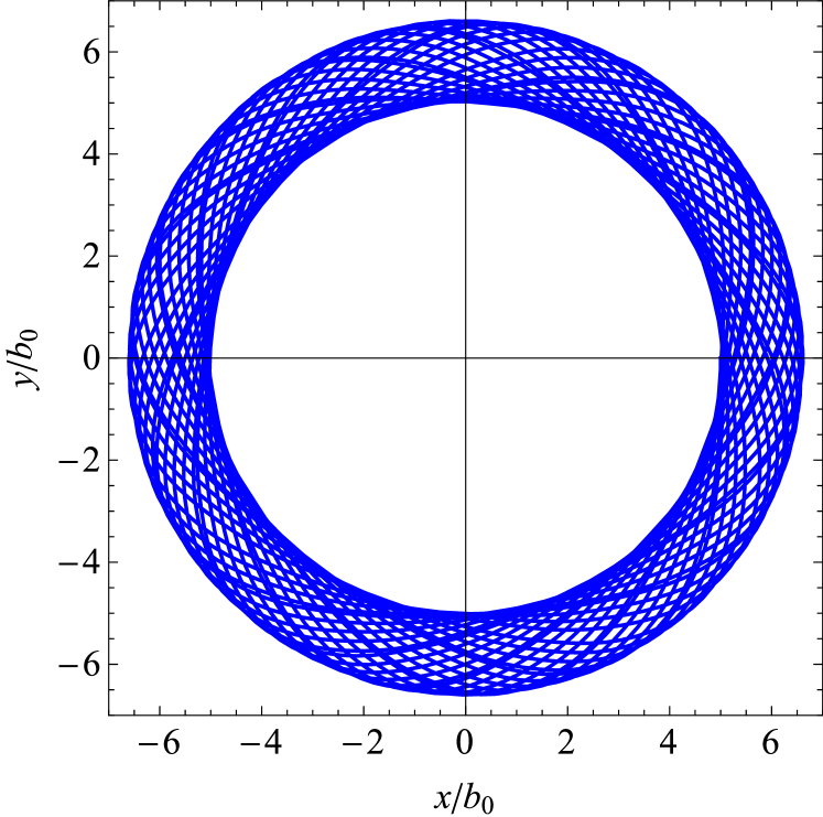
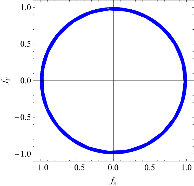
Figure 11: (a) Position of the trapped atom ${\bf r}(t)=(x(t),y(t))$ and (b) the unit vector ${\bf f}(t)=(f_{x}(t),f_{y}(t))$ parallel to the atomic orbital momentum. Here, we have taken $B_{0}=1.8V_{0}$ and initial conditions (initial position, momentum and the direction of the total atomic angular momentum), ${\bf f}(t)={\bf F}(t)/|{\bf f}(t)|$ given by Eq. (89).

It is convenient to use harmonic length and energy units:

$${\text{harmonic length}}\ \ \ \ \ \ \ \ \ b_{0}=\frac{\lambda_{0}}{2\pi}~{}\bigg{(}\frac{2{\mathcal{E}}_{0}}{V_{0}}\bigg{)}^{1/4},$$

$${\text{harmonic energy}}\ \ \ \ \ \hbar\Omega_{h}=\sqrt{\frac{{\mathcal{E}}_{0}V_{0}}{2}},$$

where the recoil energy ${\mathcal{E}}_{0}$ is

$${\mathcal{E}}_{0}=\frac{\hbar^{2}q_{0}^{2}}{2M}=\frac{2\pi^{2}\hbar^{2}}{M\lambda_{0}^{2}}.$$ (88)

In this section, we consider ⁴⁰K atoms which have $I=4$, $J=1/2$ and $F=9/2$ in the ground state. When $V_{0}=100\,{\mathcal{E}}_{0}$, $b_{0}=0.05985~{}\lambda_{0}$ and $\hbar\Omega_{h}=7.071\,{\mathcal{E}}_{0}$. The time-dependent position of the atom ${\bf r}(t)=(x(t),y(t))$ and the unit spin vector ${\bf f}(t)=(f_{x}(t),f_{y}(t))$ are shown in Fig. 11 for $B_{0}=1.8\,V_{0}$, with the following initial conditions,

$$x(0)=5~{}b_{0},\ \ \ \ \ y(0)=0,$$

$$p_{x}(0)=0,\ \ \ \ \ p_{y}(0)=-3\hbar/b_{0},$$ (89)

$$f_{x}(0)=-0.9975,\ \ \ f_{y}(0)=0.05,\ \ \ \ \ f_{z}(0)=0.05.$$

The motion of the atom is not periodic, and therefore the trajectory $(x(t),y(t))$ in Fig. 11 fills a ring with inner radius $5~{}b_{0}$ and outer radius $6.615~{}b_{0}$, whereas $(f_{x}(t),f_{y}(t))$ in Fig. 11 fills a ring with inner radius $0.9644$ and outer radius $1$. For ⁴⁰K atoms, $\lambda_{0}=766.5$ nm, and $b_{0}=45.87$ nm.

The results of this section cannot be applied to Li atoms because, for the semiclassical approximation to be valid, $F$ must be large.

Appendix E Distinguishing Between ${\bm{\Omega}}$, ${\bf a}$, ${\bf B}_{\mathrm{ex}}$

Consider a QR placed in an external magnetic field ${\bf B}_{\mathrm{ex}}$ in a non-inertial frame moving with a linear acceleration $\mathbf{a}$ and rotating with an angular velocity $\bm{\Omega}$. The 3D Hamiltonian of the QR is

$$H = H_{0}+H_{z}+H_{B}+H_{\Omega}+H_{a}.$$ (90)

Here $H_{0}$ is a 2D Hamiltonian for motion of the QR in the $x$-$y$ plane without an external magnetic field and in an inertial frame; using polar coordinates $\mathbf{r}=(r,\phi)$, $H_{0}=-\frac{\hbar^{2}\nabla^{2}}{2M}+{\tilde{V}}(r)-\tilde{B}(r)F_{r}$. The second term on the right hand side of Eq. (90), $H_{z}$, is for the motion of the trapped atom in a harmonic potential in the $z$-direction,

$$H_{z} = -\frac{\hbar^{2}\partial_{z}^{2}}{2M}+\frac{K_{z}z^{2}}{2}.$$ (91)

The harmonic oscillator force constant $K_{z}$ is assumed to be large and the atom is in the ground state of the Hamiltonian (91). The third term on the right hand side of Eq. (90), $H_{B}$, is the Zeeman interaction between the QR and the external magnetic field ${\bf B}_{\mathrm{ex}}$, $H_{B}=-\frac{g\mu_{B}}{2I+1}~{}\mathbf{F}\cdot{\bf B}_{\mathrm{ex}}$. The fourth term, $H_{\Omega}$, is due to the fictitious force in a rotating frame of reference, $H_{\Omega}=\hbar\bm{\mathcal{L}}\cdot\bm{\Omega}$, where $\bm{\mathcal{L}}=\mathbf{F}+\bm{\ell}$, and $\bm{\ell}$ is the orbital angular momentum of the atom around minimum points of $\tilde{V}(r)$. The fifth term, $H_{a}$, is due to the fictitious force appearing in a non-inertial frame moving with linear acceleration $\mathbf{a}$, $H_{a}=M\mathbf{a}\cdot\mathbf{r}$.

We shall calculate energy levels of $H_{0}+H_{z}$ in the inertial frame, and then apply first order perturbation theory in ${\bf B}_{\mathrm{ex}}$, $\bm{\Omega}$ and $\mathbf{a}$, to find the corrections to the energies of the QR.

E.1 Matrix elements of $H_{B}$

Matrix elements of $F_{x}$, $F_{y}$ and $F_{z}$ are

$$\big{\langle}n,\zeta\big{|}F_{x}\big{|}n,\zeta^{\prime}\big{\rangle} = \frac{1}{2}~{}\beta_{n,\zeta}^{\parallel}~{}\big{(}\delta_{\zeta,\zeta^{\prime}+1}+\delta_{\zeta,\zeta^{\prime}-1}\big{)},$$

$$\big{\langle}n,\zeta\big{|}F_{y}\big{|}n,\zeta^{\prime}\big{\rangle} = -\frac{i}{2}~{}\beta_{n,\zeta}^{\parallel}~{}\big{(}\delta_{\zeta,\zeta^{\prime}+1}-\delta_{\zeta,\zeta^{\prime}-1}\big{)},$$

$$\big{\langle}n,\zeta\big{|}F_{z}\big{|}n,\zeta^{\prime}\big{\rangle} = \beta_{n,\zeta}^{z}\delta_{\zeta,\zeta^{\prime}},$$

where $\langle z,\mathbf{r}|n,\zeta\rangle=\tilde{\psi}_{0}(z)\Psi_{n,\zeta}(\mathbf{r})$, and

$$\beta_{n,\zeta}^{\parallel} = \frac{1}{2}\int\Big{\{}\psi_{n,\zeta,1/2}^{2}(r)-\psi_{n,\zeta,-1/2}^{2}(r)\Big{\}}~{}dr,$$ (92)

$$\beta_{n,\zeta}^{z} = \int\psi_{n,\zeta,1/2}(r)\psi_{n,\zeta,-1/2}(r)~{}dr.$$ (93)

Note the following symmetries:

$$\beta_{n,-\zeta}^{\parallel}=\beta_{n,\zeta}^{\parallel},\qquad\beta_{n,-\zeta}^{z}=-\beta_{n,\zeta}^{z}.$$

These follow from the wave function symmetries $\psi_{n,-\zeta,1/2}(r)=\psi_{n,\zeta,1/2}(r)$ and $\psi_{n,-\zeta,-1/2}(r)=-\psi_{n,\zeta,-1/2}(r)$. The matrix elements of $H_{B}$ are

$$\big{\langle}n,\zeta\big{|}H_{B}\big{|}n,\zeta^{\prime}\big{\rangle}=-\frac{g\mu_{B}}{2I+1}~{}\bigg{\{}\zeta B_{z}\beta_{n,\zeta}^{z}\delta_{\zeta,\zeta^{\prime}}+$$

$$~{}~{}~{}~{}~{}~{}~{}~{}~{}~{}~{}~{}~{}~{}~{}\frac{\beta_{n,\zeta}^{\parallel}}{2}~{}\Big{[}B^{+}\delta_{\zeta,\zeta^{\prime}-1}+B^{-}\delta_{\zeta,\zeta^{\prime}+1}\Big{]}\bigg{\}},$$ (94)

where $B^{\pm}=B_{x}\pm iB_{y}$.

E.2 Matrix elements of $H_{\Omega}$

Matrix elements of the operator $\bm{\mathcal{L}}$ are

$$\big{\langle}n,\zeta\big{|}{\mathcal{L}}_{x}\big{|}n,\zeta^{\prime}\big{\rangle}=\big{\langle}n,\zeta\big{|}{\mathcal{L}}_{y}\big{|}n,\zeta^{\prime}\big{\rangle}=0,$$

$$\big{\langle}n,\zeta\big{|}{\mathcal{L}}_{z}\big{|}n,\zeta^{\prime}\big{\rangle}=\zeta\Omega_{z}.$$

The matrix elements of ${\mathcal{L}}_{x}$ and ${\mathcal{L}}_{y}$ vanish since the wave function $\tilde{\psi}_{0}(z)$ is even with respect to the inversion $z\to-z$, whereas ${\mathcal{L}}_{x}$ and ${\mathcal{L}}_{y}$ are odd. Hence, non-vanishing matrix elements of $H_{\Omega}$ are

$$\big{\langle}n,\zeta\big{|}H_{\Omega}\big{|}n,\zeta^{\prime}\big{\rangle} = \hbar\zeta\Omega_{z}\delta_{\zeta,\zeta^{\prime}}.$$ (95)

E.3 Matrix elements of $H_{a}$

Matrix elements of the position operator $\mathbf{r}$ are

$$\big{\langle}n,\zeta\big{|}x\big{|}n,\zeta^{\prime}\big{\rangle} = \frac{1}{2}~{}\varrho_{n,\zeta}^{\parallel}~{}\big{(}\delta_{\zeta,\zeta^{\prime}+1}+\delta_{\zeta,\zeta^{\prime}-1}\big{)},$$

$$\big{\langle}n,\zeta\big{|}y\big{|}n,\zeta^{\prime}\big{\rangle} = -\frac{i}{2}~{}\varrho_{n,\zeta}^{\parallel}~{}\big{(}\delta_{\zeta,\zeta^{\prime}+1}-\delta_{\zeta,\zeta^{\prime}-1}\big{)},$$

$$\big{\langle}n,\zeta\big{|}z\big{|}n,\zeta^{\prime}\big{\rangle} = 0,$$

where

$$\varrho_{n,\zeta}^{\parallel} = \int\Big{\{}\psi_{n,\zeta,1/2}^{2}(r)+\psi_{n,\zeta,-1/2}^{2}(r)\Big{\}}~{}rdr.$$ (96)

Note the symmetry $\varrho_{n,-\zeta}^{\parallel}=\varrho_{n,\zeta}^{\parallel}$. The matrix elements of $H_{a}$ are

$$\big{\langle}n,\zeta\big{|}H_{a}\big{|}n,\zeta^{\prime}\big{\rangle}=\frac{M\varrho_{n,\zeta}^{\parallel}}{2}~{}\Big{[}a^{+}\delta_{\zeta,\zeta^{\prime}-1}+a^{-}\delta_{\zeta,\zeta^{\prime}+1}\Big{]},$$ (97)

where $a^{\pm}=a_{x}\pm ia_{y}$.

E.4 First-order corrections to the energies

In order to find the first order corrections to the energies of the QR due to $\mathbf{B}$, $\bm{\Omega}$ and $\mathbf{a}$, we apply degenerate perturbation theory. First order corrections to the energies of the quantum states with $\zeta=\pm 1/2$ are

$$\varepsilon_{n,\pm 1/2}^{(1)}(\mathbf{B},\Omega_{z},a_{\parallel})=\pm\frac{1}{2}\Bigg{[}\bigg{(}\frac{g\mu_{B}\beta_{n,1/2}^{z}}{2I+1}~{}B_{z}+\hbar\Omega_{z}\bigg{)}^{2}+$$

$$~{}~{}~{}~{}~{}~{}~{}~{}~{}~{}~{}~{}~{}~{}~{}\Big{|}\beta_{n,1/2}^{\parallel}B^{+}+M\varrho_{n,1/2}^{\parallel}a^{+}\Big{|}^{2}\Bigg{]}^{1/2}.$$ (98)

Corrections to the energies of the quantum states with $\pm\zeta$ (where $\zeta=3/2,5/2,7/2,\ldots$) are

$$\varepsilon_{n,\pm\zeta}^{(1)}(\mathbf{B},\Omega_{z},a_{\parallel}) = \pm\zeta\bigg{(}\frac{g\mu_{B}\beta_{n,\zeta}^{z}}{2I+1}~{}B_{z}+\hbar\Omega_{z}\bigg{)}.$$ (99)

E.5 Raman Spectroscopy Considerations for Distinguishing between Various Sensors

We propose to use Raman spectroscopy to measure $\mathbf{B}$, $\bm{\Omega}$ and $\mathbf{a}$ by applying radio frequency electromagnetic waves to the QR with pump and Stokes frequencies ($\omega_{p}>\omega_{s}$) that are far-off-resonance from the $F=3/2$ atomic hyperfine state. In Sec. III.1 we discussed the Raman transition $|0,1/2\rangle\leftrightarrow|0,-1/2\rangle$ and the use of the Ramsey separated oscillating fields method to verify the Raman resonance condition $\omega\equiv\omega_{p}-\omega_{s}=\Delta_{QR}$. In order to determine ${\bm{\Omega}}$, ${\bf a}$, and ${\bf B}_{\mathrm{ex}}$, we will need to consider the Raman transitions $|0,1/2\rangle\leftrightarrow|0,-1/2\rangle$, $|0,3/2\rangle\leftrightarrow|0,5/2\rangle$ and $|0,-3/2\rangle\leftrightarrow|0,-5/2\rangle$, which have transition frequencies $\Delta_{0}\equiv\Delta_{QR}$, $\Delta_{+}$ and $\Delta_{-}$ respectively:

$$\Delta_{0} = \frac{1}{\hbar}~{}\Big{(}\varepsilon_{0,1/2}^{(1)}\big{(}\mathbf{B},\Omega_{z},a_{\parallel}\big{)}-\varepsilon_{0,-1/2}^{(1)}\big{(}\mathbf{B},\Omega_{z},a_{\parallel}\big{)}\Big{)},$$

$$\Delta_{\pm} = \frac{1}{\hbar}\Big{(}\epsilon_{0,5/2}-\epsilon_{0,3/2}+\varepsilon_{0,\pm 5/2}^{(1)}\big{(}\mathbf{B},\Omega_{z},a_{\parallel}\big{)}$$

$$-\varepsilon_{0,\pm 3/2}^{(1)}\big{(}\mathbf{B},\Omega_{z},a_{\parallel}\big{)}\Big{)}.$$

Note that when $\mathbf{B}_{\mathrm{ex}}=0$, $\bm{\Omega}=0$ and $\mathbf{a}=0$, then

$$\Delta_{+}^{(0)}=\Delta_{-}^{(0)}=\frac{1}{\hbar}~{}\big{(}\epsilon_{0,5/2}-\epsilon_{0,3/2}\big{)}.$$

We are interested in the splitting $\Delta_{1}=\Delta_{+}-\Delta_{-}$ due to $\mathbf{B}_{\mathrm{ex}}$, $\bm{\Omega}$ and $\mathbf{a}$. Using Eqs. (98) and (99), we get

$$\Delta_{0}\Big{(}B_{x},B_{y},B_{z},\Omega_{z},a_{x},a_{y};\varrho_{0,1/2}^{\parallel},\beta_{0,1/2}^{\parallel},\beta_{0,1/2}^{z}\Big{)}=$$

$$~{}~{}~{}~{}~{}~{}~{}~{}~{}~{}\frac{1}{\hbar}~{}\Bigg{[}\bigg{(}\frac{g\mu_{B}\beta_{0,1/2}^{z}}{2I+1}~{}B_{z}+\hbar\Omega_{z}\bigg{)}^{2}+$$

$$~{}~{}~{}~{}~{}~{}~{}~{}~{}~{}~{}~{}\bigg{(}\frac{g\mu_{B}\beta_{0,1/2}^{\parallel}}{2I+1}~{}B_{x}+M\varrho_{0,1/2}^{\parallel}a_{x}\bigg{)}^{2}+$$

$$~{}~{}~{}~{}~{}~{}~{}~{}~{}~{}~{}~{}\bigg{(}\frac{g\mu_{B}\beta_{0,1/2}^{\parallel}}{2I+1}~{}B_{y}+M\varrho_{0,1/2}^{\parallel}a_{y}\bigg{)}^{2}\Bigg{]}^{1/2},$$ (100)

$$\Delta_{1}\Big{(}B_{z},\Omega_{z};\beta_{0,3/2}^{z},\beta_{0,5/2}^{z}\Big{)}=\frac{1}{\hbar}~{}\bigg{\{}2\hbar\Omega_{z}+$$

$$~{}~{}~{}~{}~{}~{}~{}~{}~{}~{}~{}~{}\frac{g\mu_{B}}{2I+1}\Big{(}5\beta_{0,5/2}^{z}-3\beta_{0,3/2}^{z}\Big{)}B_{z}\bigg{\}}.$$ (101)

Nine measurements need to be made to allow determination of the 9 unknowns: $B_{z}$, $B_{y}$, $B_{z}$, $\Omega_{x}$, $\Omega_{y}$, $\Omega_{z}$, $a_{x}$, $a_{y}$ and $a_{z}$. In order to find the 9 unknowns, 9 measurements are required. In particular, measurements must be carried out with the QR placed in $x$-$y$, $y$-$z$ and $z$-$x$ optical lattices. Moreover, measurements of $\Delta_{1}$ must be made with two different laser intensities, e.g., $(V_{0},B_{0})=(100\,{\mathcal{E}}_{0},180\,{\mathcal{E}}_{0})$ and $(50\,{\mathcal{E}}_{0},90\,{\mathcal{E}}_{0})$. In other words, we consider $(V_{0},B_{0})=(10\,{\mathcal{N}}{\mathcal{E}}_{0},18\,{\mathcal{N}}{\mathcal{E}}_{0})$, where the dimensionless parameter ${\mathcal{N}}=5,10$ specifies the laser intensity. Furthermore, measurements of $\Delta_{0}$ must be made with $V_{0}=100\,{\mathcal{E}}_{0}$ and $B_{0}=180\,{\mathcal{E}}_{0}$.

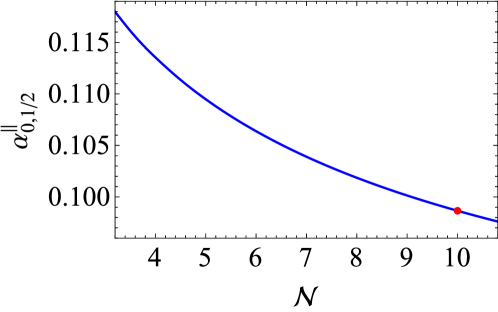
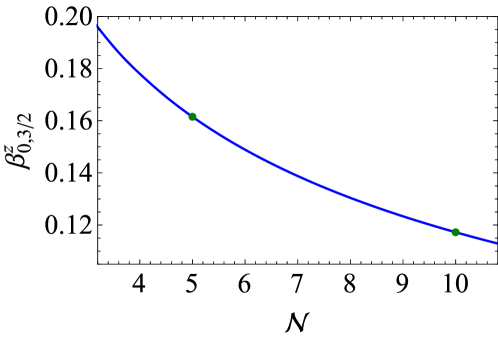
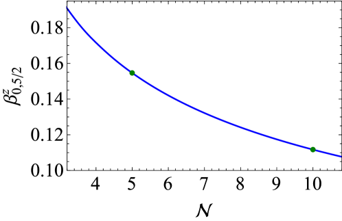
Figure 12: (a) $\beta_{0,1/2}^{z}$ (93), (b) $\beta_{0,1/2}^{\parallel}$ (92), (c) $\varrho_{0,1/2}^{\parallel}$ (96), (d) $\beta_{0,3/2}^{z}$ (93) and (e) $\beta_{0,5/2}^{z}$ (93) as functions of ${\mathcal{N}}$. The red dots denote the values of $\beta_{0,1/2}^{z}$, $\beta_{0,1/2}^{\parallel}$ and $\varrho_{0,1/2}^{\parallel}$ for ${\mathcal{N}}=10$, and the green dots denote the values of $\beta_{0,3/2}^{z}$ and $\beta_{0,5/2}^{z}$ for ${\mathcal{N}}=5$ and $10$.

The numerical solution of the Schrödinger equation (9), for different values of ${\mathcal{N}}$ yields the following results for the integrals $\beta_{0,1/2}^{z}({\mathcal{N}})$, $\beta_{0,3/2}^{z}({\mathcal{N}})$, $\beta_{0,5/2}^{z}({\mathcal{N}})$, $\beta_{0,1/2}^{\parallel}({\mathcal{N}})$ and $\varrho_{0,1/2}^{\parallel}({\mathcal{N}})$. The values of $\beta_{0,3/2}^{z}({\mathcal{N}})$ and $\beta_{0,5/2}^{z}({\mathcal{N}})$ for ${\mathcal{N}}=5,10$ are:

$$\beta_{0,3/2}^{z}(5)~{}=~{}0.161531,\ \ \ \ \ \beta_{0,3/2}^{z}(10)~{}=~{}0.117236,$$

$$\beta_{0,5/2}^{z}(5)~{}=~{}0.154678,\ \ \ \ \ \beta_{0,5/2}^{z}(10)~{}=~{}0.111702.$$

The values of $\beta_{0,1/2}^{z}(10)$, $\beta_{0,1/2}^{\parallel}(10)$ and $\varrho_{0,1/2}^{\parallel}(10)$ for ${\mathcal{N}}=10$ are:

$$\beta_{0,1/2}^{z}(10)~{}=~{}0.107807,$$

$$\beta_{0,1/2}^{\parallel}(10)~{}=~{}0.478494,$$

$$\varrho_{0,1/2}^{\parallel}(10)~{}=~{}0.0986575~{}\lambda_{0}.$$

E.6 Determining ${\bf B}_{\mathrm{ex}}$, $\bm{\Omega}$ and $\mathbf{a}$

With the optical lattice in the $x$-$y$ plane, measurements can be made of $\Delta_{1,xy}({\mathcal{N}})$ for ${\mathcal{N}}=5,10$. Two equations (one for ${\mathcal{N}}=5$ and one for ${\mathcal{N}}=10$) are thereby obtained from

$$\frac{g\mu_{B}B_{z}}{\hbar(2I+1)}\Big{(}5\beta_{0,5/2}^{z}({\mathcal{N}})-3\beta_{0,3/2}^{z}({\mathcal{N}})\Big{)}$$

$$~{}~{}~{}~{}~{}~{}~{}~{}~{}~{}~{}~{}~{}~{}~{}~{}~{}~{}+2\Omega_{z}=\Delta_{1,xy}({\mathcal{N}}).$$ (102)

The solution of these equations is

$$B_{z} = \frac{2I+1}{g\mu_{B}}~{}\frac{\hbar\big{[}\Delta_{1,xy}(10)-\Delta_{1,xy}(5)\big{]}}{\tilde{\beta}(10)-\tilde{\beta}(5)},$$ (103)

$$\Omega_{z} = \frac{\tilde{\beta}(10)~{}\Delta_{1,xy}(5)-\tilde{\beta}(5)~{}\Delta_{1,xy}(10)}{\tilde{\beta}(10)-\tilde{\beta}(5)},$$ (104)

where

$$\tilde{\beta}({\mathcal{N}}) = 5\beta_{0,5/2}^{z}({\mathcal{N}}))-3\beta_{0,3/2}^{z}({\mathcal{N}})).$$

With the optical lattice arranged in $y$-$z$ and $z$-$x$ planes, measurements can be made of $\Delta_{1,yz}({\mathcal{N}})$ and $\Delta_{1,zx}({\mathcal{N}})$ for ${\mathcal{N}}=5,10$. These measurements allow us to find $B_{x}$, $B_{y}$, $\Omega_{x}$ and $\Omega_{y}$,

$$B_{x} = \frac{2I+1}{g\mu_{B}}~{}\frac{\hbar\big{[}\Delta_{1,yz}(10)-\Delta_{1,yz}(5)\big{]}}{\tilde{\beta}(10)-\tilde{\beta}(5)},$$ (105)

$$B_{y} = \frac{2I+1}{g\mu_{B}}~{}\frac{\hbar\big{[}\Delta_{1,zx}(10)-\Delta_{1,zx}(5)\big{]}}{\tilde{\beta}(10)-\tilde{\beta}(5)},$$ (106)

$$\Omega_{x} = \frac{\tilde{\beta}(10)~{}\Delta_{1,yz}(5)-\tilde{\beta}(5)~{}\Delta_{1,yz}(10)}{\tilde{\beta}(10)-\tilde{\beta}(5)},$$ (107)

$$\Omega_{y} = \frac{\tilde{\beta}(10)~{}\Delta_{1,yz}(5)-\tilde{\beta}(5)~{}\Delta_{1,yz}(10)}{\tilde{\beta}(10)-\tilde{\beta}(5)}.$$ (108)

With the optical lattice arranged in the $x$-$y$, $y$-$z$ and $z$-$x$ planes, measurements can be made of $\Delta_{0,xy}$, $\Delta_{0,yz}$ and $\Delta_{0,zx}$ for ${\mathcal{N}}=10$. Three equations are thereby obtained,

$$\bigg{(}\frac{g\mu_{B}\beta_{0,1/2}^{\parallel}}{2I+1}~{}B_{\alpha}+M\varrho_{0,1/2}^{\parallel}a_{\alpha}\bigg{)}^{2}+$$

$$\bigg{(}\frac{g\mu_{B}\beta_{0,1/2}^{\parallel}}{2I+1}~{}B_{\alpha^{\prime}}+M\varrho_{0,1/2}^{\parallel}a_{\alpha^{\prime}}\bigg{)}^{2}+$$

$$\bigg{(}\frac{g\mu_{B}\beta_{0,1/2}^{z}}{2I+1}~{}B_{\alpha^{\prime\prime}}+\hbar\Omega_{\alpha^{\prime\prime}}\bigg{)}^{2}~{}=~{}\hbar^{2}\Delta_{0,\alpha\alpha^{\prime}}^{2},$$ (109)

where $(\alpha,\alpha^{\prime},\alpha^{\prime\prime})=(x,y,z)$, $(y,z,x)$ and $(z,x,y)$. Here $B_{\alpha}$ are given by Eqs. (103), (105) and (106) for $\alpha=z,x,y$, whereas $\Omega_{\alpha}$ are given by Eqs. (104), (107) and (108). The solution of Eq. (109) is

$$a_{x} = \frac{1}{M\varrho_{0,1/2}^{\parallel}}~{}\Bigg{\{}\frac{1}{2}~{}\sqrt{A_{x,y}+A_{z,x}-A_{y,z}}$$ (110)

$$-\frac{g\mu_{B}\beta_{0,1/2}^{\parallel}}{2I+1}~{}B_{x}\Bigg{\}},$$

$$a_{y} = \frac{1}{M\varrho_{0,1/2}^{\parallel}}~{}\Bigg{\{}\frac{1}{2}~{}\sqrt{A_{y,z}+A_{x,y}-A_{z,x}}$$ (111)

$$-\frac{g\mu_{B}\beta_{0,1/2}^{\parallel}}{2I+1}~{}B_{y}\Bigg{\}},$$

$$a_{z} = \frac{1}{M\varrho_{0,1/2}^{\parallel}}~{}\Bigg{\{}\frac{1}{2}~{}\sqrt{A_{z,x}+A_{y,z}-A_{x,y}}$$ (112)

$$-\frac{g\mu_{B}\beta_{0,1/2}^{\parallel}}{2I+1}~{}B_{z}\Bigg{\}},$$

where

$$A_{\alpha,\alpha^{\prime}} = \hbar^{2}\Delta_{0,\alpha\alpha^{\prime}}^{2}-\bigg{(}\frac{g\mu_{B}\beta_{0,1/2}^{z}}{2I+1}~{}B_{\alpha^{\prime\prime}}+\hbar\Omega_{\alpha^{\prime\prime}}\bigg{)}^{2},$$

and $(\alpha,\alpha^{\prime},\alpha^{\prime\prime})=(x,y,z)$, $(y,z,x)$ and $(z,x,y)$.

As already discussed in Sec. III.1 in connection with the far-off-resonance Raman transition $|0,1/2\rangle\leftrightarrow|0,-1/2\rangle$, to determine the Raman resonance condition $\omega_{p}-\omega_{s}=\Delta$ in all the far-off-resonance Raman processes considered in this section ($|0,1/2\rangle\leftrightarrow|0,-1/2\rangle$, $|0,3/2\rangle\leftrightarrow|0,5/2\rangle$ and $|0,-3/2\rangle\leftrightarrow|0,-5/2\rangle$), one can employ the Ramsey time-separated oscillating field method Ramsey_50 with Raman pulses Zanon .

References

- (1) S. Sachdev, Quantum Phase Transitions, 2nd Ed., (Cambridge University Press, Cambridge, 2011), pp. 12-14.
- (2) https://en.wikipedia.org/wiki/Quantum_rotor_model
- (3) L. Allen, et al., Phys. Rev. A 45, 8185 (1992).
- (4) M.A. Clifford, J. Arlt, J. Courtial, K. Dholakia, Optics Communications 156, 300 (1998).
- (5) L. Amico, A. Osterloh and F. Cataliotti, Phys. Rev. Lett. 95, 063201 (2005).
- (6) A. Kumar et al., New J. Phys. 18, 025001 (2016).
- (7) Y.-J. Lin, K. Jimnez-Garca, and I. B. Spielman, Nature 471, 83-86 (2011).
- (8) A.M. Dudarev, R.B. Diener, I. Carusotto, Q. Niu, Phys. Rev. Lett. 92, 153005 (2004).
- (9) F. Le Kien, P. Schneeweiss and A. Rauschenbeutel, Eur. Phys. J. D 67, 92 (2013).
- (10) Strictly speaking, when atoms have and , the high order terms within perturbation theory in powers of the electric field generate tensor interactions (quadrupole, octupole, etc.) of the atoms with the SDOLP. However, within second order perturbation theory (as used here in our paper), just scalar and vector potentials appear for atoms with and any (even ).
- (11) V. Galitski, I. B. Spielman, Nature 494, 49 (2013).
- (12) G. Juzeliunas, J. Ruseckas, J. Dalibard, Phys. Rev. A 81, 053403 (2010).
- (13) X.-J. Liu, K. T. Law, T. K. Ng, Phys. Rev. Lett. 112, 086401 (2014).
- (14) C. Zhang, S. Tewari, R. Lutchyn, S. Das Sarma, Phys. Rev. Lett. 101, 160401 (2008).
- (15) It is also of interest to explore SDOLP with other symmetries.
- (16) C. Cohen-Tannoudji and J. Dupont-Roc, Phys. Rev. A 5, 968 (1972).
- (17) J. H. Becher, S. Baier, K. Aikawa, M. Lepers, J.-F. Wyart, O. Dulieu, and F. Ferlaino, Phys. Rev. A 97, 012509 (2018).
- (18) One could do a full band-structure calculation, but our interest is in the lowest energy states with negligible well to well tunneling and wave functions localized at small , hence the 2D isotropic approximation is sufficient.
- (19) S. G. Karshenboim and V. G. Ivanov, Phys. Lett. B 524, 259 (2002).
- (20) C. Weitenberg, M. Endres, J. F. Sherson, M. Cheneau, P. Schauß, T. Fukuhara, I. Bloch, St. Kuhr, Nature 471, 319 (2011).
- (21) C. Cohen-Tannoudji and S. Reynaud, J. Phys. A: Math. Gen. 10 345, 365 (1977).
- (22) V. V. Sokolov and V. G. Zelevinsky, Ann. Phys. 216, 323 (1992).
- (23) N. F. Ramsey, Phys. Rev. 78, 695 (1950).
- (24) T. Zanon-Willette et al., Phys. Rev. A 90, 053427 (2014).
- (25) D. Budker and M. Romalis, Nature Physics 3, 227 (2007).
- (26) V. B. Berestetskii, E. M. Lifshitz, and L. P. Pitaevskii, Course of Theoretical Physics, Volume 4: Relativistic Quantum Theory, 2nd Ed., (Pergamon, 1982), p. 153-155.
- (27) D. Budker, D. F. J. Kimball, Optical Magnetometry, (Cambridge University Press, 2013), pp. 4-5.
- (28) L. Viverit, C. Menotti, T. Calarco, and A. Smerzi, Phys. Rev. Lett.93, 110401 (2004).
- (29) I. Bloch, J. Dalibard, W. Zwerger, Rev. Mod. Phys. 80, 885 (2008).
- (30) L. J. Radziemsky, R. Engleman Jr., and J. W. Brault, Phys. Rev. A 52, 4462 (1995).
- (31) H. Al-Taiy, N. Wenzel, S. Preußler, J. Klinger, and T. Schneider, Opt. Lett. 39, 5826 (2014).