Joint Dynamic Pricing and Radio Resource Allocation Framework for IoT Services

Abstract

In this paper, we study the problem of resource allocation as well as pricing in the context of Internet of things (IoT) networks. We provide a novel pricing model for IoT services where all the parties involved in the communication scenario as well as their revenue and cost are determined. We formulate the resource allocation in the considered model as a multi-objective optimization problem where in addition to the resource allocation variables, the price values are also optimization variables. To solve the proposed multi-objective optimization problem, we use the scalarization method which gives different Pareto optimal solutions. We solve the resulting problems using the alternating approach based on the successive convex approximation (SCA) method which converges to a local solution with few iterations. We also consider a conventional approach where each entity tries to maximize its own revenue independently. Simulation results indicate that by applying the proposed joint framework, we can increase the total revenue compared to the conventional case while providing an almost complete fairness among the players. This is while the conventional approach fails to provide such a fairness.
Index Terms– IoT,  Resource Allocation,  Pricing,  SCMA,  HetNets.

I Introduction

I-A Motivation

Internet of Things (IoT) is a framework that allows billions of smart devices to be connected to the Internet [1]. Such devices are able to operate and transmit data to other systems with minimal or without any human interaction. The development of IoT has greatly influenced many areas, and many IoT applications have been implemented to improve quality of life in different aspects such as health care, transportation, and manufacturing [2]. There are different business models of wireless network virtualization which are described in [3] as two-level and four-level models. In two-level model, mobile network operators (MNO) and service provider (SP) act as logical players after wireless network virtualization. All of the infrastructures and physical resources are operated by MNOs based on virtualization decisions. SPs operate on virtual resources to offer end-to-end services to end users. In four-level model, the roles of MNO and SP are decoupled into more specialized tasks, i.e., MNO consists of InP and mobile virtual network provider (MVNP), and SP consists of mobile virtual network operator (MVNO) and SP where MVNO assigns the virtual resources to SPs and SP concentrates on providing services to its end users based on MVNOs decisions. In this paper, the MNO becomes InP and SPs will create and deploy the virtual resource to provide end-to-end services based on two-level model. The core of most IoT systems contains smart wireless sensors that can collect data from the environment and convey such data to the central controllers, referred to as IoT service provider (ISP), for further processing [1]. The entity that owns such sensors is referred to as the sensor device owner (SDO). In addition to SDO and ISP, we can generally consider 4 other essential units: infrastructure providers (InPs), the regulatory, power supplier, and end users. InP provides the required infrastructures and equipments for the communications of different ISPs and lends bandwidth to them, regulatory lends bandwidth to different InPs, and power supplier provides the necessary electrical power in base stations (BS) and sensors. Finally, the ISP processes the raw data transmitted by sensors and sells them to end users. As all of these mentioned entities in an IoT network have their own technical and financial interests, reaching a financial resource sharing agreement among them is usually a challenging task. Moreover, most small SDO’s and ISPs may not have enough knowledge on the technical and financial details of the service provided by the large InPs and may be billed by the InP’s at unreasonable rates. The lack of a transparent market and solid pricing model is one of the main barriers that prevent IoT from becoming pervasive. Therefore, a solid trading/pricing model is necessary to regulate such deals among InPs, ISPs, SDO, and end users. Moreover, IoT in fifth generation (5G) network is required to be able support massive machine type communication. Massive machine type communication requires enormous amounts of connectivity capability and high spectral efficiency.

I-B Related Work

There are a number of works in wireless networking literature that use pricing methods to model the trade-offs among different entities [4, 5]. Examples include secondary and primary operators in cognitive radio networks [6], device to device (D2D) communications [7], and different base stations in heterogeneous networks [8]. The existing literature focuses on bandwidth as the resource to be traded [9].

In D2D communication, user equipments transmit data signals to each other over a direct link using the cellular resources rather than the BS to improve bandwidth efficiency. In fact, existing cellular users can sustain their network resources by switching to the D2D mode. Therefore, there must be some incentive or reward for the D2D users to make them interested to do so. This requires proper pricing strategies for operators to obtain maximum possible profit as shown in [10, 11, 12, 13]. In a cognitive radio network, the primary cellular network owns the licensed spectrum while the secondary users attempt to dynamically utilize the spectrum. In most cases, such dynamic occupation requires users to pay for the services they get from the primary network through direct billing or by serving as primary users’ (PU) relays. Thus, the spectrum becomes a special kind of commodity in a CRN [14]. Consequently, a large amount of research has been done to provide different pricing strategies to accommodate efficient spectrum sharing [15, 16, 17, 18, 19, 20, 21, 22, 23]. The idea of heterogeneous networks in which low-cost small cells (e.g., microcells, picocells, and femtocells) with small coverage areas and low transmission powers are deployed is a promising one for improving the efficiency of spectrum utilization in cellular networks. In this regard, pricing schemes have been considered in [24, 25, 26, 27, 28, 29, 30, 31].

Few papers in the literature have considered pricing schemes for resources other than spectrum. In D2D communications, power has been considered as a subject of trading in [32]. In [33] a D2D communication framework is considered in which the authors design a power-pricing framework based on the principle of the Stackelberg game. In [34], relay servers are a subject of pricing where sellers offer cooperative services at the cost of resources such as power by way of auction.

As far as pricing in IoT is concerned, only few works exist in the literature [35, 36, 37, 38, 39]. As a simple market, [35] investigates the pricing scheme in a business model of IoT with three participants: multiple sensing data owners, service providers, and users. With similar market components, [36] proposes an economic model in big data and IoT in which the authors use the classification-based machine learning algorithms to define the generic utility function of data. Then, using a Stackelberg game, the optimal raw data selling price is obtained. Service management of an IoT device has been investigated in [37] where the Markov decision process is used to model an optimization framework in order to obtain an optimal policy for the device owner. This policy considers energy transfer and bid acceptance, and attempts to maximize the reward, defined as the revenue from a winning bid and the costs paid for energy transfer. The authors of [39] consider a cloud based system including IoT subscriber and propose a threshold based approach to decide the pricing and allocation of virtual machines to sequentially arriving requests in order to maximize the revenue of the cloud service provider over a finite time horizon.

The authors of [40] propose a hierarchical mobile edge computing architecture based on the LTE advanced networks. They study two time scale mechanisms to allocate the computing and communications resources. In the computing resources allocation, they consider an auction-based pricing model to maximize the utility of the service provider where the price of each virtual machine is updated at the beginning of each frame. To solve this problem, they apply a heuristic algorithm. Moreover, they propose a centralized optimal solution based on Lagrange multipliers for the bandwidth allocation. The authors of [41] consider a fog computing based system as an appropriate choice to provide low latency services. The considered network consists of a few data service operators each of which controls several fog nodes. The fog nodes provide the required data service to a set of subscribers. They formulate a Stackelberg game to study the pricing model for the data service operators as well as the resource allocation problem for the subscribers. They proposed a many-to-many matching game to investigate the pairing problem between data service operators and fog nodes. Moreover, they applied another layer of many-to-many matching between the paired fog nodes and serving data service subscribers.

Despite its necessity, there is no pricing platform in the IoT literature that can comprehensively address the idea of resource sharing/trading which can happen at multiple levels. Motivated by the aforementioned discussion, the objective of this paper is to provide an end to end dynamic pricing and power and subcarrier allocation framework in IoT systems that facilitates reaching an agreement between the network elements and in particular, SDO, InPs, ISPs, and end users, and to create transparency in such agreements.

I-C Our Contributions

To address the conflicting interests of different players, we have to take into account each entity’s objective. Consequently, there are multiple objectives in the network design process which should be optimized simultaneously. Since we have both integer and continuous variables, in order to jointly maximize the revenues of major players in the proposed pricing model, we use the multi-objective approach which is a powerful tool that can address such a scenario.

The novelty of the proposed model is two-fold:

• A novel comprehensive framework including all the major players and different levels of resource sharing is provided. To the best of our knowledge, no prior work exists that addresses this complex and multilevel pricing structure of IoT systems.

• To solve the proposed end to end optimization problem, several tools including multi-objective optimization, convex optimization and relaxation methods are combined in the framework of wireless communications.

We evaluate the performance of the proposed model for different values of the network parameters using simulations. Moreover, we compare the performance of the proposed algorithm to the conventional approach, in which resource allocation and pricing are disjointly performed by each IoT player. From simulations, we can find out that the proposed joint approach leads to much more fairness than the conventional one as the values of the utility functions of involving players are much closer to each other than those of conventional approach.

The organization of the paper is as follows: In Section II, the system model and the pricing scheme are presented. In Section III, problem formulation is provided. Solution of the proposed problem is provided in Section V and simulation results are in Section VIII. Finally, the paper is concluded in Section IX.

II System Model

II-A Network Model

Consider a scenario with $U$ users, each of which belongs to one ISP and acts as an IoT service consumer, and $I$ InPs, where InP $i$ has $B_{i}$ BSs. On the other hand, there are $S_{b_{i}}$ sensors in the coverage area of BS $b_{i}$ who sell the raw data to ISPs. Also each InP framework contains one macro base station (MBS) and few femto base stations (FBSs). In this paper, we focus on both the uplink and downlink transmission of raw data which is based on frequency division duplex (FDD). The uplink transmission of raw data is the transmission from sensors to BSs which is shown at Fig. 1. The downlink transmission is the transmission of processed data from BSs to users which is shown at Fig. 2. The data processing is performed at the private cloud of each ISP which is connected to all BSs.

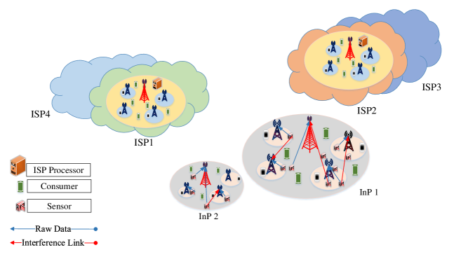
Figure 1: Uplink transmission from sensors to BSs.

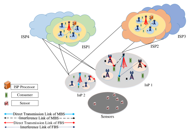
Figure 2: Downlink transmission from BSs to users.

We denote the set of InPs by $\mathcal{I}=\{1,2,\dots,I\}$, set of BSs in InP $i$ by $\mathcal{B}_{i}=\{1,2,\dots,B_{i}\}$, and set of sensors by $\mathcal{S}=\bigcup\limits_{b_{i}\in\mathcal{B}_{i}}\mathcal{S}_{b_{i}}$, where $\mathcal{S}_{b_{i}}$ is the set of sensors in cell $b_{i}$ whose cardinality is $S_{b_{i}}$. Besides, there are $U$ users with the set of $\mathcal{U}=\{1,2,\dots,U\}$, each of which can be associated to only one BS in the network. Moreover, each user is served by one ISP. The set of ISPs is denoted by $\mathcal{V}=\{1,2,\dots,V\}$. Furthermore, the set of users served by ISP $v$ is denoted by $\mathcal{K}_{v}$. Hence, we have $\mathcal{U}=\bigcup\limits_{v\in\mathcal{V}}\mathcal{K}_{v}$. The frequency bandwidth of downlink and uplink wireless channels in each InP $i$ are denoted by $W^{\text{Dn}}_{i}$ and $W^{\text{Up}}_{i}$, respectively. We assume that different InPs use non-overlapping bandwidth. Within each InP_i, the bandwidth is divided between downlink and uplink transmission, denoted by $W^{\text{Dn}}_{i}$ and $W^{\text{Up}}_{i}$, respectively. These available spectrum are divided into $N_{i}$ and $M_{i}$ subcarriers, respectively. It is assumed that each subcarrier has bandwidth of $W_{\text{S}}$. The set of downlink and uplink subcarriers in InP $i$ are indicated by $\mathcal{N}_{i}=\{1,2,\dots,N_{i}\}$ and $\mathcal{M}_{i}=\{1,2,\dots,M_{i}\}$, respectively. We utilize the SCMA technique which is one of the main candidates for 5G multiple access techniques [42, 43, 44]. We assume that the set of downlink and uplink codebooks are shown by $\mathcal{DC}_{i}=\{1,\dots,C_{i}\}$ and $\mathcal{UC}_{i}=\{1,\dots,C^{\prime}_{i}\}$, respectively, where $C_{i}$ and $C^{\prime}_{i}$ are the number of downlink and uplink codebooks, respectively. Moreover, the mapping between downlink subcarriers and codebooks is shown by $q^{c_{i}}_{n}$, where $q^{c_{i}}_{n}=1$ if codebook $c_{i}$ consists of subcarrier $n$, and otherwise $q^{c_{i}}_{n}=0$. In a same way, for uplink case we define $q^{\prime c^{\prime}_{i}}_{m}$ to show the mapping between uplink subcarriers and codebooks. It should be noted that for both uplink and downlink cases, we assume that the mapping between codebooks and subcarriers is known and fixed. Let $p^{c_{i}}_{b_{i},u}$ denote the downlink transmit power of BS $b_{i}\in\mathcal{B}_{i}$ to user $u$ on codebook $c_{i}\in\mathcal{DC}_{i}$, and $p^{\prime c^{\prime}_{i}}_{b_{i},s_{b_{i}}}$ denotes the uplink transmit power of sensor $s_{b_{i}}$ to BS $b_{i}$ on codebook $c^{\prime}_{i}$. The channel gain between BS $b_{i}$ and user $u$ on subcarrier $n$, and between BS $b_{i}$ and sensor $s_{b_{i}}$ on subcarrier $m$ are determined by $h^{n}_{b_{i},u}$ and $h^{m}_{b_{i},s_{b_{i}}}$, respectively. The codebook assignment indicators are expressed by $\rho^{c_{i}}_{b_{i},u},\rho^{\prime c^{\prime}_{i}}_{b_{i},s_{b_{i}}}\in\{0,1\}$. Note that $p^{c_{i}}_{b_{i},u}$ is assigned to subcarrier $n$ based on a given proportion $0\leq\lambda^{b_{i}}_{n,c_{i}}\leq 1$, indicated based on codebook design which satisfies $\sum_{n\in\mathcal{C}_{i}}\lambda^{b_{i}}_{n,c_{i}}=1$ where $\mathcal{C}_{i}$ is the set of subcarriers in codebook $c_{i}$. In a same way, $p^{\prime c^{\prime}_{i}}_{b_{i},s_{b_{i}}}$ is assigned to subcarrier $m$ based on a given proportion $\lambda^{\prime b_{i}}_{m,c_{i}}$. The definitions of all variables are summarized in Table I.

TABLE I: NOTATIONS

Notation	Description	$\bm{L}^{\text{Power,BS}}$	$[L^{\text{Power,BS}}_{b_{i}}]$
$\phi^{\text{InP,Power}}_{i}$	Income of InP $i$ from lending power to ISPs	$\bm{p}^{\text{BS}}$	$[p^{c_{i}}_{b_{i},u}]$
$\phi^{\text{InP,BW}}_{i}$	income of InP $i$ from lending spectrum to ISPs and sensors	$\bm{p}^{\text{Sens}}$	$[p^{c^{\prime}_{i}}_{b_{i},s_{b_{i}}}]$
$\psi^{\text{InP,Power}}_{i}$	Cost of InP $i$ for buying power from power suppliers	$\bm{\rho}^{\text{BS}}$	$[\rho^{c_{i}}_{b_{i},u}]$
$\psi^{\text{InP,BW}}_{i}$	Cost of buying bandwidth from regulatory with unit price $C^{\text{BW}}_{i}$	$\bm{\rho}^{\text{Sens}}$	$[\rho^{\prime c^{\prime}_{i}}_{b_{i},s_{b_{i}}}]$
$\psi^{\text{ISP,Power}}_{v}$	Cost of buying power from InPs at ISP $v$	$\bm{L}^{\text{BW}}$	$[L^{\text{BW}}_{i}]$
$\Phi^{\text{InP}}_{\text{tot}}$	Total revenue of InPs in the network	$\bm{L}^{\text{Sens,Data}}$	$[L^{\text{Sens,Data}}_{v,s_{b_{i}}}]$
$\psi^{\text{ISP,BW}}_{v}$	cost of buying bandwidth from InPs at ISP $v$	$\bm{L}^{\text{Up,Rate}}$	$[L^{\text{Up,Rate}}_{s_{b_{i}}}]$
$\psi^{\text{ISP,data}}_{v}$	Price of buying the raw data from sensors at each ISP $v$	$\bm{L}^{\text{Dn,Rate}}$	$[L^{\text{Dn,Rate}}_{v}]$
$\phi^{\text{ISP,rate}}_{v}$	Income of ISP $v$ originating from the data service	$\bm{\alpha}$	$[\alpha_{s_{b_{i}},u}]$
$\phi^{\text{ISP,data}}_{v}$	Income of ISP $v$ from selling the processed data to users	$\bm{L}^{\text{Reserv,User}}$	$[L^{\text{Reserv,User}}_{v,u}]$
$q^{c_{i}}_{n}$	$q^{c_{i}}_{n}=1$ if codebook $c_{i}$ consists of subcarrier $n$, $q^{c_{i}}_{n}=0$ otherwise	$\mathcal{I}$	Set of InPs
$q^{\prime c^{\prime}_{i}}_{m}$	$q^{\prime c^{\prime}_{i}}_{m}=1$ if codebook $c^{\prime}_{i}$ consists of subcarrier $m$, $q^{c_{i}}_{m}=0$ otherwise	$\mathcal{B}_{i}$	Set of BSs in InP $i$
$p^{c_{i}}_{b_{i},u}$	Downlink transmit power of BS $b_{i}\in\mathcal{B}_{i}$ to user $u$ on codebook $c_{i}$	$\mathcal{S}$	Set of sensors
$p^{\prime c^{\prime}_{i}}_{b_{i},s_{b_{i}}}$	Uplink transmit power of sensor $s_{b_{i}}$ to BS $b_{i}$ on codebook $c^{\prime}_{i}$	$\mathcal{S}_{b_{i}}$	Set of sensors in cell $b_{i}$
$h^{n}_{b_{i},u}$	Channel gain between BS $b_{i}$ and user $u$ on subcarrier $n$	$\mathcal{U}$	Set of users
$h^{m}_{b_{i},s_{b_{i}}}$	Channel gain between BS $b_{i}$ and sensor $s_{b_{i}}$ on subcarrier $m$	$\mathcal{V}$	Set of ISPs
$\rho^{c_{i}}_{b_{i},u}$	Downlink codebook assignment	$\mathcal{N}_{i}$	Set of downlink subcarriers
$\rho^{\prime c^{\prime}_{i}}_{b_{i},s_{b_{i}}}$	Uplin codebook assignment	$\mathcal{M}_{i}$	Set of uplink subcarriers
$\gamma^{c_{i}}_{b_{i},u}$	SINR at user $u$ from BS $b_{i}$ on codebook $c_{i}$	$\mathcal{DC}_{i}$	Set of downlink codebooks
$r^{c_{i}}_{b_{i},u}$	Data rate at user $u$ from BS $b_{i}$ on codebook $c_{i}$	$\mathcal{UC}_{i}$	Set of uplink codebooks
$\gamma^{c^{\prime}_{i}}_{b_{i},s_{b_{i}}}$	SINR from sensor $s_{b_{i}}$ to BS $b_{i}$ on subcarrier $m$	$\Phi^{\text{InP}}_{i}$	Revenue of InP $i$
$r^{c^{\prime}_{i}}_{b_{i},s_{b_{i}}}$	Data rate at BS $b_{i}$ from sensor $s_{b_{i}}$ on codebook $c^{\prime}_{i}$	$\Phi^{\text{Sens}}_{s_{b_{i}}}$	Revenue of each sensor $s_{b_{i}}$
$P^{\text{max}}_{b_{i}}$	Maximum allowable transmit power of each BS $b_{i}$	$\Phi^{\text{Sens}}_{\text{tot}}$	Total revenue of sensors
$P^{\text{Bat}}_{s_{b_{i}}}$	Maximum allowable transmit power of each sensor $s_{b_{i}}$	$\Phi^{\text{ISP}}_{v}$	Revenue of each ISP $v$
$R^{\text{min}}_{\text{Dn},v}$	Minimum sum data rate of users owned by ISP $v$	$\Phi^{\text{ISP}}_{\text{tot}}$	Total revenue of ISPs
$R^{\text{min}}_{\text{Up},s_{b_{i}}}$	Minimum required data rate at each sensor $s_{b_{i}}$ for uplink	$\psi^{\text{ISP,Uplink}}_{v}$	Paid money from ISP $v$ to SDO
$\phi^{\text{User,data}}_{u}$	Reward of user $u$ for IoT service
$\psi^{\text{User,rate}}_{u}$	Received data rate by users which is offered by ISP $v$

The received SINR at user $u$ from BS $b_{i}$ on codebook $c_{i}$ is given by

$$\gamma^{c_{i}}_{b_{i},u}=\dfrac{\rho^{c_{i}}_{b_{i},u}\sum_{n\in\mathcal{N}_{i}}q^{c_{i}}_{n}\lambda^{b_{i}}_{n,c_{i}}p^{c_{i}}_{b_{i},u}|h^{n}_{b_{i},u}|^{2}}{I^{c_{i}}_{b_{i},u}+(\sigma^{c_{i}}_{b_{i},u})^{2}},$$ (1)

where $I^{c_{i}}_{b_{i},u}$ is obtained by

$$I^{c_{i}}_{b_{i},u}=\sum_{b^{\prime}_{i}\in\mathcal{B}_{i}/\{b_{i}\}}\sum_{u^{\prime}\in\mathcal{U}}\sum_{n\in\mathcal{N}_{i}}\rho^{c_{i}}_{b^{\prime}_{i},u^{\prime}}q^{c_{i}}_{n}\lambda^{b^{\prime}_{i}}_{n,c_{i}}p^{c_{i}}_{b^{\prime}_{i},u^{\prime}}|h^{n}_{b^{\prime}_{i},u}|^{2}.$$ (2)

Accordingly, the data rate at user $u$ from BS $b_{i}$ on codebook $c_{i}$ is formulated by $r^{c_{i}}_{b_{i},u}=\log_{2}(1+\gamma^{c_{i}}_{b_{i},u}).$ The uplink SINR from sensor $s_{b_{i}}$ to BS $b_{i}$ on subcarrier $m$ can be expressed by

$$\gamma^{c^{\prime}_{i}}_{b_{i},s_{b_{i}}}=\dfrac{\rho^{\prime c^{\prime}_{i}}_{b_{i},s_{b_{i}}}\sum_{m\in\mathcal{M}_{i}}q^{\prime m}_{b_{i}}\lambda^{\prime b_{i}}_{n,c^{\prime}_{i}}p^{\prime c^{\prime}_{i}}_{b_{i},s_{b_{i}}}|h^{m}_{b_{i},s_{b_{i}}}|^{2}}{I^{\prime c^{\prime}_{i}}_{b_{i},s_{b_{i}}}+(\sigma^{\prime c^{\prime}_{i}}_{b_{i},s_{b_{i}}})^{2}},$$ (3)

where $I^{\prime c^{\prime}_{i}}_{b_{i},s_{b_{i}}}$ is given by

$$I^{\prime c^{\prime}_{i}}_{b_{i},s_{b_{i}}}=\sum_{b^{\prime}_{i}\in\mathcal{B}_{i}/\{b_{i}\}}\sum_{s^{\prime}_{b^{\prime}_{i}}\in\mathcal{S}_{b_{i}}}\sum_{m\in\mathcal{M}_{i}}\rho^{\prime c^{\prime}_{i}}_{b^{\prime}_{i},s^{\prime}_{b^{\prime}_{i}}}q^{c^{\prime}_{i}}_{m}\lambda^{\prime b^{\prime}_{i}}_{m,c^{\prime}_{i}}p^{\prime c^{\prime}_{i}}_{b^{\prime}_{i},s^{\prime}_{b^{\prime}_{i}}}|h^{m}_{b_{i},s^{\prime}_{b^{\prime}_{i}}}|^{2}.$$ (4)

The received data rate at BS $b_{i}$ from sensor $s_{b_{i}}$ on codebook $c^{\prime}_{i}$ is thus formulated by $r^{c^{\prime}_{i}}_{b_{i},s_{b_{i}}}=\log_{2}(1+\gamma^{c^{\prime}_{i}}_{b_{i},s_{b_{i}}}).$ The following two constraints ensure that each user selects one BS in the network:

$$\rho^{c_{i}}_{b_{i},u}+\rho^{c^{\prime\prime}_{i^{\prime}}}_{b_{i^{\prime}}^{\prime},u}\leq 1,\forall i,i^{\prime}\in\mathcal{I},i^{\prime}\neq i,b_{i}\in\mathcal{B}_{i},b_{i^{\prime}}^{\prime}\in\mathcal{B}_{i^{\prime}},u\in\mathcal{U},c_{i}\in\mathcal{DC}_{i},c^{\prime\prime}_{i^{\prime}}\in\mathcal{DC}_{i^{\prime}},$$ (5)

$$\rho^{c_{i}}_{b_{i},u}+\rho^{c^{\prime\prime\prime}_{i}}_{b_{i}^{\prime},u}\leq 1,\forall i\in\mathcal{I},b_{i},b_{i}^{\prime}\in\mathcal{B}_{i},b_{i}^{\prime}\neq b_{i},u\in\mathcal{U},c_{i},\ c^{\prime\prime\prime}_{i}\in\mathcal{DC}_{i}.$$ (6)

In SCMA, each subcarrier can at most be reused $K$ times, therefore, the following constraints are enforced for downlink and uplink, respectively:

$$\sum_{b_{i}\in\mathcal{B}_{i}}\sum_{u\in\mathcal{U}}\sum_{c_{i}\in\mathcal{DC}_{i}}\rho^{c_{i}}_{b_{i},u}q^{c_{i}}_{n}\leq K,\forall i\in\mathcal{I},n\in\mathcal{N}_{i},$$ (7)

$$\sum_{b_{i}\in\mathcal{B}_{i}}\sum_{s_{b_{i}}\in\mathcal{S}_{i}}\sum_{c^{\prime}_{i}\in\mathcal{UC}_{i}}\rho^{\prime c^{\prime}_{i}}_{b_{i},s_{b_{i}}}q^{\prime c^{\prime}_{i}}_{m}\leq K,\forall i\in\mathcal{I},m\in\mathcal{M}_{i}.$$ (8)

Maximum allowable transmit power of each BS $b_{i}$ and sensor $s_{b_{i}}$ are denoted by $P^{\text{max}}_{b_{i}}$ and $P^{\text{Bat}}_{s_{b_{i}}}$, respectively. Hence, we have

$$\sum_{u\in\mathcal{U}}\sum_{c_{i}\in\mathcal{C}_{i}}\rho^{c_{i}}_{b_{i},u}p^{c_{i}}_{b_{i},u}\leq P^{\text{max}}_{b_{i}},\forall i\in\mathcal{I},b_{i}\in\mathcal{B}_{i},$$ (9)

$$\sum_{c^{\prime}_{i}\in\mathcal{UC}_{i}}\rho^{c^{\prime}_{i}}_{b_{i},s_{b_{i}}}p^{c^{\prime}_{i}}_{b_{i},s_{b_{i}}}\leq P^{\text{Bat}}_{s_{b_{i}}},\forall i\in\mathcal{I},b_{i}\in\mathcal{B}_{i},s_{b_{i}}\in\mathcal{S}_{b_{i}}.$$ (10)

According to the different user rate requirements of various ISPs, we have the following minimum required data rate constraints as:

$$\sum_{i\in\mathcal{I}}\sum_{b_{i}\in\mathcal{B}_{i}}\sum_{c_{i}\in\mathcal{DC}_{i}}r^{c_{i}}_{b_{i},u}\geq R^{\text{min}}_{\text{Dn},v},\forall v\in\mathcal{V},u\in\mathcal{K}_{v},$$ (11)

where $R^{\text{min}}_{\text{Dn},v}$ is the minimum sum data rate of users owned by ISP $v$. In the same way, we have a minimum data rate constraint for each sensor as:

$$\sum_{c_{i}\in\mathcal{UC}_{i}}r^{c^{\prime}_{i}}_{b_{i},s_{b_{i}}}\geq R^{\text{min}}_{\text{Up},s_{b_{i}}},\forall b_{i}\in\mathcal{B}_{i},s_{b_{i}}\in\mathcal{S}_{b_{i}},$$ (12)

where $R^{\text{min}}_{\text{Up},s_{b_{i}}}$ is the minimum required data rate at each sensor $s_{b_{i}}$ for uplink transmission.

II-B Pricing Scheme

In the proposed pricing model, each sensor sells its raw sensed data to ISPs. In other words, each ISP collects data from different sensors. Then, ISPs perform a processing based on the determined sets of collected data and sell it to users. Fig. 3 illustrates the proposed pricing model of the considered system.

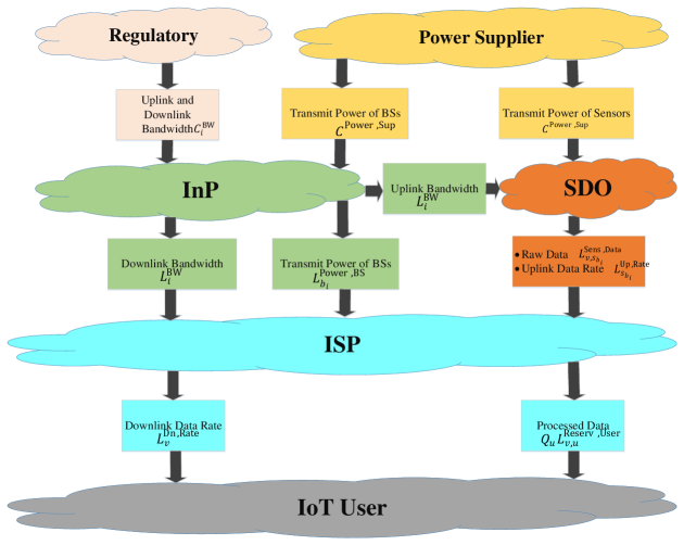
Figure 3: IoT Pricing Scheme.

Based on Fig. 3, there are four major players in the proposed IoT pricing scheme: InPs, sensors, ISPs and users. In the following, we present the pricing model of each player.

II-B1 InPs

Each InP leases power and bandwidth from a power supplier and regulatory, respectively, and lends them to ISPs. In addition, each InP $i$ lends its bandwidth to the set of sensors owned by BSs in $\mathcal{B}_{i}$. Assume that $L^{\text{Power,BS}}_{b_{i}}$ let the unit of price of power consumption at BS $b_{i}$, per Watt. The income of InP $i$ from lending power to ISPs can be obtained as

$$\phi^{\text{InP,Power}}_{i}=\sum_{b_{i}\in\mathcal{B}_{i}}\sum_{u\in\mathcal{U}}\sum_{c_{i}\in\mathcal{DC}_{i}}L^{\text{Power,BS}}_{b_{i}}\rho^{c_{i}}_{b_{i},u}p^{c_{i}}_{b_{i},u}.$$ (13)

Let $L^{\text{BW}}_{i}$ denote the unit price for lending downlink and uplink transmission bandwidths, per Hz, to ISPs and sensors. Therefore, the income of InP $i$ from lending spectrum to ISPs and sensors are given by

$$\phi^{\text{InP,BW}}_{i}=\sum_{b_{i}\in\mathcal{B}_{i}}\sum_{u\in\mathcal{U}}\sum_{c_{i}\in\mathcal{DC}_{i}}\sum_{n\in\mathcal{N}_{i}}q^{c_{i}}_{n}L^{\text{BW}}_{i}\rho^{c_{i}}_{b_{i},u}W_{\text{S}}+$$ (14)

$$\sum_{b_{i}\in\mathcal{B}_{i}}\sum_{s_{b_{i}}\in\mathcal{S}_{b_{i}}}\sum_{c^{\prime}_{i}\in\mathcal{UC}_{i}}\sum_{m\in\mathcal{M}_{i}}q^{\prime m}_{b_{i}}L^{\text{BW}}_{i}\rho^{c^{\prime}_{i}}_{b_{i},s_{b_{i}}}W_{\text{S}}.$$

The cost of InP $i$ for buying power from power suppliers with a unit price $C^{\text{Power,Sup}}$ (per Watt) is obtained by

$$\psi^{\text{InP,Power}}_{i}=\sum_{b_{i}\in\mathcal{B}_{i}}\sum_{u\in\mathcal{U}}\sum_{c_{i}\in\mathcal{C}_{i}}\rho^{c_{i}}_{b_{i},u}p^{c_{i}}_{b_{i},u}C^{\text{Power,Sup}},\forall i\in\mathcal{I},$$ (15)

and the cost of buying bandwidth from regulatory with unit price $C^{\text{BW}}_{i}$ (per Hz) can be formulated by

$$\psi^{\text{InP,BW}}_{i}=W^{\text{Dn}}_{i}C^{\text{BW}}_{i}+W^{\text{Up}}_{i}C^{\text{BW}}_{i},\forall i\in\mathcal{I}.$$ (16)

The revenue of InP $i$ is thus given by

$$\Phi^{\text{InP}}_{i}=\phi^{\text{InP,Power}}_{i}+\phi^{\text{InP,BW}}_{i}-\psi^{\text{InP,Power}}_{i}-\psi^{\text{InP,BW}}_{i}.$$ (17)

Hence, the total revenue of InPs in the network is formulated as $\Phi^{\text{InP}}_{\text{tot}}=\sum_{i\in\mathcal{I}}\Phi^{\text{InP}}_{i}.$

II-B2 Sensors

Each sensor $s_{b_{i}}$ has a reservation wage cost $C^{\text{Sens,Reserv}}_{s_{b_{i}}}$ to obtain the raw data. Moreover, it leases power from the power supplier and bandwidth from InPs with units price $C^{\text{Power,Sup}}$ (per Watt) and $L^{\text{BW}}_{i}$ (per Hz), respectively, to sell the raw data with the price $L^{\text{Sens,Data}}_{v,s_{b_{i}}}$ which is offered by ISP $v$ to sensor $s_{b_{i}}$ in uplink transmission to ISPs. In doing so, the uplink data rate of each sensor $s_{b_{i}}$ is the income of the sensor with unit of price $L^{\text{Up,Rate}}_{s_{b_{i}}}$ (1/bps). Accordingly, the revenue of each sensor $s_{b_{i}}$ can be obtained by

$$\Phi^{\text{Sens}}_{s_{b_{i}}}=\sum\limits_{v\in\mathcal{V}}\min\{\sum\limits_{u\in\mathcal{K}_{v}}\alpha_{s_{b_{i}},u},1\}L^{\text{Sens,Data}}_{v,s_{b_{i}}}+\sum\limits_{v\in\mathcal{V}}\sum_{c^{\prime}_{i}\in\mathcal{UC}_{i}}\min\{\sum\limits_{u\in\mathcal{K}_{v}}\alpha_{s_{b_{i}},u},1\}r^{c^{\prime}_{i}}_{b_{i},s_{b_{i}}}L^{\text{Up,Rate}}_{s_{b_{i}}}$$ (18)

$$-\min\{\sum\limits_{u\in\mathcal{U}}\alpha_{s_{b_{i}},u},1\}C^{\text{Sens,Reserv}}_{s_{b_{i}}}-\sum\limits_{c^{\prime}_{i}\in\mathcal{UC}_{i}}\rho^{c^{\prime}_{i}}_{b_{i},s_{b_{i}}}p^{c^{\prime}_{i}}_{b_{i},s_{b_{i}}}C^{\text{Power,Sup}}-\sum_{c^{\prime}_{i}\in\mathcal{UC}_{i}}\sum_{m\in\mathcal{M}_{i}}q^{\prime m}_{b_{i}}\rho^{c^{\prime}_{i}}_{b_{i},s_{b_{i}}}W_{\text{S}}L^{\text{BW}}_{i},$$

where the binary indicator $\alpha_{s_{b_{i}},u}\in\{0,1\}$ takes value $1$ when the raw data of sensor $s_{b_{i}}$ is used in the processing data of user $u$ at the cloud of ISP. Note that each ISP buys the data of sensor $s_{b_{i}}$ at most once. The total revenue of sensors is thus given by $\Phi^{\text{Sens}}_{\text{tot}}=\sum_{s_{b_{i}}\in\mathcal{S}_{b_{i}}}\Phi^{\text{Sens}}_{s_{b_{i}}}.$

II-B3 ISPs

Each ISP buys power and downlink bandwidth from InP with unit price $L^{\text{Power,BS}}_{b_{i}}$ and $L^{\text{BW}}_{i}$, respectively. Moreover, it leases the raw data of sensors with price $L^{\text{Sens,Data}}_{v,s_{b_{i}}}$ and gives money to sensors for their uplink data rate with the unit price $L^{\text{Up,Rate}}_{s_{b_{i}}}$. The income of each ISP is composed of two components. Firstly, they get money for their downlink data rate servicing to users with the unit of price $L^{\text{Dn,Rate}}_{v}$ (per bit/s). Secondly, they lend their processed data to users. The price of the processed data which is served to user $u$ from ISP $v$ is $Q_{u}L^{\text{Reserv,User}}_{v,u}$, where $Q_{u}=q\log(1+\frac{\sum\limits_{i=1}^{I}\sum\limits_{b_{i}\in\mathcal{B}_{i}}\sum\limits_{s_{b_{i}}\in\mathcal{S}_{b_{i}}}\alpha_{s_{b_{i}},u}}{\sum\limits_{i=1}^{I}\sum\limits_{b_{i}\in\mathcal{B}_{i}}S_{b_{i}}})$ is the service quality function of a set of sensors whose data is used by user $u$ [4], and $L^{\text{Reserv,User}}_{v,u}$ is the maximum reservation price that ISP $v$ takes from user $u$. In addition, $q$ is a sensing quality of player that is used to tune service quality received by the users. In doing so, the income of ISP $v$ originating from the data service given to the its subscribing users is given by

$$\phi^{\text{ISP,rate}}_{v}=\sum_{i\in\mathcal{I}}\sum_{b_{i}\in\mathcal{B}_{i}}\sum_{u\in\mathcal{K}_{v}}\sum_{c_{i}\in\mathcal{DC}_{i}}\sum_{n\in\mathcal{N}_{i}}q^{c_{i}}_{n}L^{\text{Dn,Rate}}_{v}W_{\text{S}}r^{c_{i}}_{b_{i},u}.$$ (19)

Moreover, the income of ISP $v$ from selling the processed data to users in $\mathcal{K}_{v}$ is obtained by $\phi^{\text{ISP,data}}_{v}=\sum_{u\in\mathcal{K}_{v}}Q_{u}L^{\text{Reserv,User}}_{v,u}.$ The cost of buying power from InPs at ISP $v$ is given by

$$\psi^{\text{ISP,Power}}_{v}=\sum_{i\in\mathcal{I}}\sum_{b_{i}\in\mathcal{B}_{i}}\sum_{u\in\mathcal{K}_{v}}\sum_{c_{i}\in\mathcal{DC}_{i}}L^{\text{Power,BS}}_{b_{i}}\rho^{c_{i}}_{b_{i},u}p^{c_{i}}_{b_{i},u},$$ (20)

and the cost of buying bandwidth from InPs at ISP $v$ is given by

$$\psi^{\text{ISP,BW}}_{v}=\sum_{i\in\mathcal{I}}\sum_{b_{i}\in\mathcal{B}_{i}}\sum_{u\in\mathcal{K}_{v}}\sum_{c_{i}\in\mathcal{DC}_{i}}\sum_{n\in\mathcal{N}_{i}}q^{c_{i}}_{n}L^{\text{BW}}_{i}\rho^{c_{i}}_{b_{i},u}W_{\text{S}}.$$ (21)

The price of buying the raw data from sensors at each ISP $v$ can be formulated by

$$\psi^{\text{ISP,data}}_{v}=\sum_{s_{b_{i}}\in\mathcal{S}_{b_{i}}}\min\{\sum\limits_{u\in\mathcal{K}_{v}}\alpha_{s_{b_{i}},u},1\}L^{\text{Sens,Data}}_{v,s_{b_{i}}}.$$ (22)

Moreover, each ISP $v$ gives money to SDO for their uplink data rates with the total price of

$$\psi^{\text{ISP,Uplink}}_{v}=\sum_{i\in\mathcal{I}}\sum_{b_{i}\in\mathcal{B}_{i}}\sum_{s_{b_{i}}\in\mathcal{S}_{b_{i}}}\min\{\sum\limits_{u\in\mathcal{K}_{v}}\alpha_{s_{b_{i}},u},1\}r^{c^{\prime}_{i}}_{b_{i},s_{b_{i}}}L^{\text{Up,Rate}}_{s_{b_{i}}}.$$ (23)

The revenue of each ISP $v$ is thus formulated as follows:

$$\Phi^{\text{ISP}}_{v}=\phi^{\text{ISP,rate}}_{v}+\phi^{\text{ISP,data}}_{v}-\psi^{\text{ISP,Power}}_{v}-\psi^{\text{ISP,BW}}_{v}-\psi^{\text{ISP,data}}_{v}-\psi^{\text{ISP,Uplink}}_{v}.$$ (24)

Therefore, the total revenue of ISPs is given by $\Phi^{\text{ISP}}_{\text{tot}}=\sum_{v\in\mathcal{V}}\Phi^{\text{ISP}}_{v}.$

II-B4 Users

Each user is willing to achieve the high quality IoT and high data rate services with low power and spectrum consumption. Therefore, for each user, rewards and costs are modeled as follows:

• Reward 1: IoT service (the processed data) is received by users with unit price $C^{\text{Reserv,User}}_{u}$. Therefore, reward of user $u$ for IoT service is given by

  $$\phi^{\text{User,data}}_{u}=Q_{u}C^{\text{Reserv,User}}_{u},\forall u\in\mathcal{K}_{v}.$$ (25)

• Cost 1: The received data rate by users which is offered by ISP $v$ with unit cost $L^{\text{Dn,Rate}}_{v}$ is given by

  $$\psi^{\text{User,rate}}_{u}=\sum_{i\in\mathcal{I}}\sum_{b_{i}\in\mathcal{B}_{i}}\sum_{c_{i}\in\mathcal{DC}_{i}}\sum_{n\in\mathcal{N}_{i}}q^{c_{i}}_{n}L^{\text{Dn,Rate}}_{v}W_{\text{S}}r^{c_{i}}_{b_{i},u},\forall u\in\mathcal{K}_{v}.$$ (26)

• Cost 2: IoT service price at user $u$ with unit cost $L^{\text{Reserv,User}}_{v,u}$ which is offered by ISP $v$ to user $u$, can be obtained by $Q_{u}L^{\text{Reserv,User}}_{v,u},\forall u\in\mathcal{K}_{v}$.

The revenue of each user $u\in\mathcal{K}_{v}$ is formulated as follows:

$$\Phi^{\text{User}}_{u}=\phi^{\text{User,data}}_{u}-\psi^{\text{User,rate}}_{u}-Q_{u}L^{\text{Reserv,User}}_{v,u},\forall u\in\mathcal{K}_{v}.$$ (27)

Therefore, the total revenue of users is obtained by $\Phi^{\text{User}}_{\text{tot}}=\sum_{u\in\mathcal{U}}\Phi^{\text{User}}_{u}.$

III Proposed pricing Model

In this paper, we aim to design a joint uplink/downlink data delivery policy with BS selection at users and determine the efficient value of pricing units offered by each player. Moreover, we obtain the efficient raw data subset selection for processing the collected raw data for each user. Let us denote $\bm{p}=[\bm{p}^{\text{BS}},\bm{p}^{\text{Sens}}]$, $\bm{p}^{\text{BS}}=[p^{c_{i}}_{b_{i},u}]$, $\bm{p}^{\text{Sens}}=[p^{c^{\prime}_{i}}_{b_{i},s_{b_{i}}}]$, $\bm{\rho}=[\bm{\rho}^{\text{BS}},\bm{\rho}^{\text{Sens}}]$, $\bm{\rho}^{\text{BS}}=[\rho^{c_{i}}_{b_{i},u}]$, $\bm{\rho}^{\text{Sens}}=[\rho^{\prime c^{\prime}_{i}}_{b_{i},s_{b_{i}}}]$, $\bm{L}^{\text{Power,BS}}=[L^{\text{Power,BS}}_{b_{i}}]$, $\bm{L}^{\text{BW}}=[L^{\text{BW}}_{i}]$, $\bm{L}^{\text{Sens,Data}}=[L^{\text{Sens,Data}}_{v,s_{b_{i}}}]$, $\bm{L}^{\text{Up,Rate}}=[L^{\text{Up,Rate}}_{s_{b_{i}}}]$, $\bm{L}^{\text{Dn,Rate}}=[L^{\text{Dn,Rate}}_{v}]$, $\bm{\alpha}=[\alpha_{s_{b_{i}},u}]$, $\bm{L}^{\text{Reserv,User}}=[L^{\text{Reserv,User}}_{v,u}]$, $\bm{L}=[\bm{L}^{\text{Power,BS}},\bm{L}^{\text{BW}},\bm{L}^{\text{Sens,Data}},$
$\bm{L}^{\text{Up,Rate}},\bm{L}^{\text{Dn,Rate}},\bm{L}^{\text{Reserv,User}}]$. Since we have both integer and continuous variables, in order to jointly maximize the revenues of the different players, we use the multi-objective approach. The multi-objective optimization problem of the proposed system model is formulated as

$$\max_{\bm{\rho},\bm{p},\bm{L},\bm{\alpha}}\{\Phi^{\text{ISP}}_{\text{tot}},\Phi^{\text{InP}}_{\text{tot}},\Phi^{\text{Sens}}_{\text{tot}},\Phi^{\text{User}}_{\text{tot}}\},\text{s.t.}:\hskip 7.11317pt\eqref{cons userassociation dn1}\text{-}\eqref{cons min rate user up}.$$ (28)

The proposed optimization problem in (28) is intractable. To tackle this issue, we adopt the scalarization method. By using this method, a multi-objective function can be transformed into a simple, tractable, and single objective function [45, 46, 47]. Note that there are many cases in the scalarization methods resulting in different Pareto optimal solutions. The result of solution of each single objective problem forms a point of Pareto boundary. In the following, we exploit two approaches within the scalarization method, namely, max-min and weighted-one algorithms, to solve the multi-objective optimization problem. The main reasons behind selection of these methods are that the weighted-one is very simple and the max-min method achieves the best fairness in the system. For more clarification please refer to Appendix A.

III-A Max-Min Approach

ISPs, InPs, and SDO are three players which work together to provide IoT services for end users. In this approach, our goal is to maximize the fairness index among these three players. Consequently, our max-min optimization problem is formulated as follows:

$$\max_{\bm{\rho},\bm{p},\bm{L},\bm{\alpha}}\min_{\text{ISP},\text{InP},\text{Sens},}\{\Phi^{\text{ISP}}_{\text{tot}},\Phi^{\text{InP}}_{\text{tot}},\Phi^{\text{Sens}}_{\text{tot}}\}+\Phi^{\text{User}}_{\text{tot}},\text{s.t.}:\hskip 7.11317pt\eqref{cons userassociation dn1}\text{-}\eqref{cons min rate user up}.$$ (29)

III-B Weight-One Approach

In this approach, our goal is to maximize the summation of weighted utilities of ISPs, InPs, sensors, and users. The max-min optimization problem is formulated as follows:

$$\max_{\bm{\rho},\bm{p},\bm{L},\bm{\alpha}}\sum_{v\in\mathcal{V}}\omega^{\text{ISP}}_{v}\Phi^{\text{ISP}}_{v}+\sum_{u\in\mathcal{U}}\omega^{\text{User}}_{u}\Phi^{\text{User}}_{u}+\sum_{i\in\mathcal{I}}\omega^{\text{InP}}_{i}\Phi^{\text{InP}}_{i}+\sum_{i\in\mathcal{I}}\sum_{b_{i}\in\mathcal{B}_{i}}\sum_{s_{b_{i}}\in\mathcal{S}_{b_{i}}}\omega^{\text{Sens}}_{s_{b_{i}}}\Phi^{\text{Sens}}_{s_{b_{i}}}$$ (30a)

$$\text{s.t.}\hskip 2.84544pt\eqref{cons userassociation dn1}\text{-}\eqref{cons min rate user up}.$$

where $\omega^{\text{ISP}}_{v}$, $\omega^{\text{User}}_{u}$, $\omega^{\text{InP}}_{i}$ and $\omega^{\text{Sens}}_{s_{b_{i}}}$ are the weights tuned based on the priority of $\Phi^{\text{ISP}}_{v}$, $\Phi^{\text{User}}_{u}$, $\Phi^{\text{InP}}_{i}$ and $\Phi^{\text{Sens}}_{s_{b_{i}}}$, respectively.

IV Conventional Approach in IoT Pricing

Based on a conventional approach, each player by considering a minimum utility requirement for the other players maximizes its utility. Then, the calculated results of its corresponding price variables are reported to a central unit. Central unit by considering the reported price variables solves a comprehensive joint power and codebook allocation problem for all of the players. Consequently, by the conventional method, price variables are determined by players and power and codebook are assigned centrally. In the following, the optimization problems which should be solved by different players and the optimization problem which should be solved by the central unit are presented. It should be noted that each InP can play the role of the central unit to solve the comprehensive joint power and codebook allocation problem.

IV-A InP Optimization Problem

Each InP maximizes its utility function by considering minimum utilities $\Phi^{\text{ISP}}_{0}$, $\Phi^{\text{User}}_{0}$ and $\Phi^{\text{SDO}}_{0}$ for ISPs, users and SDO, respectively. Moreover, for other InPs it considers minimum utility $\Phi^{\text{EInP}}_{0}$. The corresponding optimization problem is formulated as:

$$\max_{\bm{\rho},\bm{p},\bm{L},\bm{\alpha}}\Phi^{\text{InP}}_{i},$$ (31a)

$$\text{s.t.}:\hskip 7.11317pt\eqref{cons userassociation dn1}\text{-}\eqref{cons min rate user up},$$

$$\hskip 28.45274pt\Phi^{\text{ISP}}_{\text{tot}}\geq\Phi^{\text{ISP}}_{0},$$ (31b)

$$\hskip 28.45274pt\Phi^{\text{User}}_{\text{tot}}\geq\Phi^{\text{User}}_{0},$$ (31c)

$$\hskip 28.45274pt\Phi^{\text{InP}}_{i^{\prime}}\geq\Phi^{\text{EInP}}_{0},i^{\prime}\in\mathcal{I}/i,$$ (31d)

$$\hskip 28.45274pt\Phi^{\text{SDO}}_{\text{tot}}\geq\Phi^{\text{SDO}}_{0}.$$ (31e)

IV-B ISP Optimization Problem

Each ISP maximizes its utility function by considering minimum utilities $\Phi^{\text{InP}}_{0}$, $\Phi^{\text{User}}_{0}$ and $\Phi^{\text{SDO}}_{0}$ for InPs, users and SDO, respectively. Moreover, for other ISPs, each ISP considers minimum utility $\Phi^{\text{EISP}}_{0}$. The corresponding optimization problem is formulated as:

$$\max_{\bm{\rho},\bm{p},\bm{L},\bm{\alpha}}\Phi^{\text{ISP}}_{v},$$ (32a)

$$\text{s.t.}:\hskip 7.11317pt\eqref{cons userassociation dn1}\text{-}\eqref{cons min rate user up},$$

$$\hskip 28.45274pt\Phi^{\text{InP}}_{\text{tot}}\geq\Phi^{\text{InP}}_{0},$$ (32b)

$$\hskip 28.45274pt\Phi^{\text{User}}_{\text{tot}}\geq\Phi^{\text{User}}_{0},$$ (32c)

$$\hskip 28.45274pt\Phi^{\text{ISP}}_{v^{\prime}}\geq\Phi^{\text{EISP}}_{0},\forall v^{\prime}\in\mathcal{V}/v,$$ (32d)

$$\hskip 28.45274pt\Phi^{\text{SDO}}_{\text{tot}}\geq\Phi^{\text{SDO}}_{0}.$$ (32e)

IV-C SDO Optimization Problem

SDO maximizes its utility function by considering minimum utilities $\Phi^{\text{InP}}_{0}$, $\Phi^{\text{User}}_{0}$ and $\Phi^{\text{ISP}}_{0}$ for InPs, users, and ISPs, respectively. The corresponding optimization problem is formulated as:

$$\max_{\bm{\rho},\bm{p},\bm{L},\bm{\alpha}}\Phi^{\text{SDO}}_{\text{tot}},$$ (33a)

$$\text{s.t.}:\hskip 7.11317pt\eqref{cons userassociation dn1}\text{-}\eqref{cons min rate user up},$$

$$\hskip 28.45274pt\Phi^{\text{InP}}_{\text{tot}}\geq\Phi^{\text{InP}}_{0},$$ (33b)

$$\hskip 28.45274pt\Phi^{\text{User}}_{\text{tot}}\geq\Phi^{\text{User}}_{0},$$ (33c)

$$\hskip 28.45274pt\Phi^{\text{ISP}}_{\text{tot}}\geq\Phi^{\text{ISP}}_{0}.$$ (33d)

IV-D Central Unit Optimization Problem

As we mentioned, central unit by considering the reported prices, solves a joint power and codebook allocation problem. Therefore, optimization problem which should be solved by the central unit is presented as follows:

$$\max_{\bm{\rho},\bm{p},\bm{\alpha}}\{\Phi^{\text{ISP}}_{\text{tot}},\Phi^{\text{InP}}_{\text{tot}},\Phi^{\text{Sens}}_{\text{tot}},\Phi^{\text{User}}_{\text{tot}}\},\text{s.t.}:\hskip 7.11317pt\eqref{cons userassociation dn1}\text{-}\eqref{cons min rate user up}.$$ (34)

V Solution

V-A Solution of the Weight-One Approach

In order to solve the optimization problem (30), the alternating algorithm is used [48]. Based on the alternating method, in each iteration, each set of variables are calculated assuming other variable sets are fixed.

The main solution steps are presented in Algorithm 1.

Algorithm 1 ITERATIVE RESOURCE ALLOCATION ALGORITHM

• STEP1: Initialization:

  • Set $t=0$ (iteration number),

  • Find $\bm{\alpha}(0)$, $\mathbf{P}(0)$, $\mathbf{L}(0)$, and $\bm{\rho}(0)$

• STEP2:

  • Set $\mathbf{P}=\mathbf{P}(t)$, $\bm{\alpha}=\bm{\alpha}(t)$, and $\bm{\rho}=\bm{\rho}(t)$,

  • Solve the optimization problem with variable $\mathbf{L}$,

  • Set the result of optimization problem solution to $\mathbf{L}(t+1)$,

• STEP3:

  • Set $\mathbf{P}=\mathbf{P}(t)$, $\mathbf{L}=\mathbf{L}(t+1)$, and $\bm{\rho}=\bm{\rho}(t)$,

  • Solve the optimization problem with variable $\bm{\alpha}$,

  • Set the result of optimization problem solution to $\bm{\alpha}(t+1)$,

• STEP4:

  • Set $\mathbf{L}=\mathbf{L}(t+1)$, $\bm{\alpha}=\bm{\alpha}(t+1)$, and $\bm{\rho}=\bm{\rho}(t)$,

  • Solve the optimization problem with variable $\mathbf{P}$,

  • Set the result of optimization problem solution to $\mathbf{P}(t+1)$,

• STEP5:

  • Set $\mathbf{L}=\mathbf{L}(t+1)$, $\bm{\alpha}=\bm{\alpha}(t+1)$, and $\mathbf{P}=\mathbf{P}(t+1)$,

  • Solve the optimization problem with variable $\bm{\rho}$,

  • Set the result of optimization problem solution to $\bm{\rho}(t+1)$,

• STEP6:

  • If convergence
    stop and return $\bm{\alpha}$, $\mathbf{P}$, $\mathbf{L}$, and $\bm{\rho}$ as the suboptimal solution,

  • Else
    set $t=t+1$ and go back to STEP 2,

  • Output:   Suboptimal value of $\bm{\alpha}$, $\mathbf{P}$, $\mathbf{L}$, and $\bm{\rho}$.

In Step 2, the problem of finding $\bm{L}$ is solved by assuming the other variables being fixed. This problem is a non-constrained linear programming which can be solved by using the CVX toolbox [49]. The optimization problem with variable $\bm{L}$ is formulated as follows:

$$\max_{\bm{L}}\sum_{v\in\mathcal{V}}\omega^{\text{ISP}}_{v}\Phi^{\text{ISP}}_{v}+\sum_{u\in\mathcal{U}}\omega^{\text{User}}_{u}\Phi^{\text{User}}_{u}$$ (35)

$$+\sum_{i\in\mathcal{I}}\omega^{\text{InP}}_{i}\Phi^{\text{InP}}_{i}+\sum_{i\in\mathcal{I}}\sum_{b_{i}\in\mathcal{B}_{i}}\sum_{s_{b_{i}}\in\mathcal{S}_{b_{i}}}\omega^{\text{Sens}}_{s_{b_{i}}}\Phi^{\text{Sens}}_{s_{b_{i}}}.$$

In Step 3, with assumption of other optimization variables being fixed, the problem of finding $\bm{\alpha}$ is solved. By using the epigraph technique and relaxing the variable $\bm{\alpha}$ to have the continuous value between $0$ and $1$, the optimization problem (35) is reformulated as:

$$\max_{\bm{\alpha},\bm{\delta},\bm{\beta}}\sum_{i\in\mathcal{I}}\sum_{b_{i}\in\mathcal{B}_{i}}\sum_{s_{b_{i}}\in\mathcal{S}_{b_{i}}}\omega^{\text{Sens}}_{s_{b_{i}}}\bigg{(}\sum\limits_{v\in\mathcal{V}}\delta_{v,s_{b_{i}}}L^{\text{Sens,Data}}_{v,s_{b_{i}}}+\sum\limits_{v\in\mathcal{V}}\sum\limits_{c^{\prime}_{i}\in\mathcal{UC}_{i}}\delta_{v,s_{b_{i}}}r^{c^{\prime}_{i}}_{b_{i},s_{b_{i}}}L^{\text{Up,Rate}}_{s_{b_{i}}}-\beta_{s_{b_{i}}}C^{\text{Sens,Reserv}}_{s_{b_{i}}}\bigg{)}+$$

$$\sum_{v\in\mathcal{V}}\omega^{\text{ISP}}_{v}\bigg{(}\sum_{u\in\mathcal{K}_{v}}q\log(1+\frac{\sum\limits_{i=1}^{I}\sum\limits_{b_{i}\in\mathcal{B}_{i}}\sum\limits_{s_{b_{i}}\in\mathcal{S}_{b_{i}}}\alpha_{s_{b_{i}},u}}{\sum\limits_{i=1}^{I}\sum\limits_{b_{i}\in\mathcal{B}_{i}}S_{b_{i}}})L^{\text{Reserv,User}}_{v,u}-\sum_{s_{b_{i}}\in\mathcal{S}_{b_{i}}}\delta_{v,s_{b_{i}}}L^{\text{Sens,Data}}_{v,s_{b_{i}}}-$$

$$\sum_{i\in\mathcal{I}}\sum_{b_{i}\in\mathcal{B}_{i}}\sum_{s_{b_{i}}\in\mathcal{S}_{b_{i}}}\delta_{v,s_{b_{i}}}r^{c^{\prime}_{i}}_{b_{i},s_{b_{i}}}L^{\text{Up,Rate}}_{s_{b_{i}}}\bigg{)}+\sum_{v\in\mathcal{V}}\sum_{u\in\mathcal{K}_{v}}\omega^{\text{User}}_{u}\bigg{(}q\log(1+\frac{\sum\limits_{i=1}^{I}\sum\limits_{b_{i}\in\mathcal{B}_{i}}\sum\limits_{s_{b_{i}}\in\mathcal{S}_{b_{i}}}\alpha_{s_{b_{i}},u}}{\sum\limits_{i=1}^{I}\sum\limits_{b_{i}\in\mathcal{B}_{i}}S_{b_{i}}})$$

$$(C^{\text{Reserv,User}}_{u}-L^{\text{Reserv,User}}_{v,u})\bigg{)},$$

$$\text{s.t.}\leavevmode\nobreak\ \leavevmode\nobreak\ \leavevmode\nobreak\ \delta_{v,s_{b_{i}}}\leq\sum\limits_{u\in\mathcal{K}_{v}}\alpha_{s_{b_{i}},u},$$ (36a)

$$\leavevmode\nobreak\ \leavevmode\nobreak\ \leavevmode\nobreak\ \leavevmode\nobreak\ \leavevmode\nobreak\ \leavevmode\nobreak\ \delta_{v,s_{b_{i}}}\leq 1,$$ (36b)

$$\leavevmode\nobreak\ \leavevmode\nobreak\ \leavevmode\nobreak\ \leavevmode\nobreak\ \leavevmode\nobreak\ \leavevmode\nobreak\ \beta_{s_{b_{i}}}\leq\sum\limits_{u\in\mathcal{U}}\alpha_{s_{b_{i}},u},$$ (36c)

$$\leavevmode\nobreak\ \leavevmode\nobreak\ \leavevmode\nobreak\ \leavevmode\nobreak\ \leavevmode\nobreak\ \leavevmode\nobreak\ \beta_{s_{b_{i}}}\leq 1,$$ (36d)

$$\leavevmode\nobreak\ \leavevmode\nobreak\ \leavevmode\nobreak\ \leavevmode\nobreak\ \leavevmode\nobreak\ \leavevmode\nobreak\ 0\leq\alpha_{s_{b_{i}},u}\leq 1,$$ (36e)

where $\bm{\delta}=[\delta_{v,s_{b_{i}}}]$ and $\bm{\beta}=[\beta_{s_{b_{i}}}]$ are the auxiliary variables corresponding to the epigraph algorithm. The optimization problem (36) is convex which can be solved by applying the CVX toolbox. The aim of Step 4 is finding $\bm{p}$. The corresponding optimization problem is formulated as:

$$\max_{\bm{p}}\sum_{v\in\mathcal{V}}\omega^{\text{ISP}}_{v}\bigg{(}\sum_{i\in\mathcal{I}}\sum_{b_{i}\in\mathcal{B}_{i}}\sum_{u\in\mathcal{K}_{v}}\sum_{c_{i}\in\mathcal{DC}_{i}}L^{\text{Dn,Rate}}_{v}W_{\text{S}}r^{c_{i}}_{b_{i},u}$$ (37a)

$$-\sum_{i\in\mathcal{I}}\sum_{b_{i}\in\mathcal{B}_{i}}\sum_{u\in\mathcal{K}_{v}}\sum_{c_{i}\in\mathcal{DC}_{i}}L^{\text{Power,BS}}_{b_{i}}\rho^{c_{i}}_{b_{i},u}p^{c_{i}}_{b_{i},u}-$$

$$\sum_{i\in\mathcal{I}}\sum_{b_{i}\in\mathcal{B}_{i}}\sum_{s_{b_{i}}\in\mathcal{S}_{b_{i}}}\min\{\sum\limits_{u\in\mathcal{K}_{v}}\alpha_{s_{b_{i}},u},1\}r^{c^{\prime}_{i}}_{b_{i},s_{b_{i}}}L^{\text{Up,Rate}}_{s_{b_{i}}}\bigg{)}-$$

$$\sum_{v\in\mathcal{V}}\sum_{u\in\mathcal{K}_{v}}\omega^{\text{User}}_{u}\bigg{(}\sum_{i\in\mathcal{I}}\sum_{b_{i}\in\mathcal{B}_{i}}\sum_{c_{i}\in\mathcal{DC}_{i}}L^{\text{Dn,Rate}}_{v}W_{\text{S}}r^{c_{i}}_{b_{i},u}\bigg{)}+$$

$$\sum_{i\in\mathcal{I}}\omega^{\text{InP}}_{i}\bigg{(}\sum_{b_{i}\in\mathcal{B}_{i}}\sum_{u\in\mathcal{U}}\sum_{c_{i}\in\mathcal{DC}_{i}}L^{\text{Power,BS}}_{b_{i}}\rho^{c_{i}}_{b_{i},u}p^{c_{i}}_{b_{i},u}\bigg{)}+$$

$$\sum_{i\in\mathcal{I}}\sum_{b_{i}\in\mathcal{B}_{i}}\sum_{s_{b_{i}}\in\mathcal{S}_{b_{i}}}\omega^{\text{Sens}}_{s_{b_{i}}}\bigg{(}\sum\limits_{v\in\mathcal{V}}\sum\limits_{c^{\prime}_{i}\in\mathcal{UC}_{i}}\min\{\sum\limits_{u\in\mathcal{K}_{v}}\alpha_{s_{b_{i}},u},1\}$$

$$r^{c^{\prime}_{i}}_{b_{i},s_{b_{i}}}L^{\text{Up,Rate}}_{s_{b_{i}}}-\sum\limits_{c^{\prime}_{i}\in\mathcal{UC}_{i}}\rho^{c^{\prime}_{i}}_{b_{i},s_{b_{i}}}p^{c^{\prime}_{i}}_{b_{i},s_{b_{i}}}C^{\text{Power,Sup}}\bigg{)},$$

$$\text{s.t.}\hskip 2.84544pt\eqref{cons max power BS}\text{-}\eqref{cons min rate user up}.$$

Due to the non-convex rate function in uplink and downlink transmissions, the optimization problem (37) is non-convex. To tackle the non-convexity issue of the considered problem, a successive convex approximation (SCA) approach with difference of two concave functions (D.C.) approximation method is used. In order to apply this method, at first the downlink rate function is written as $r^{c_{i}}_{b_{i},u}=f^{c_{i}}_{b_{i},u}-g^{c_{i}}_{b_{i},u},$ where

$$f^{c_{i}}_{b_{i},u}=\log_{2}(\rho^{c_{i}}_{b_{i},u}\sum_{n\in\mathcal{N}_{i}}q^{c_{i}}_{n}\lambda^{b_{i}}_{n,c_{i}}p^{c_{i}}_{b_{i},u}|h^{n}_{b_{i},u}|^{2}+I^{c_{i}}_{b_{i},u}+(\sigma^{c_{i}}_{b_{i},u})^{2}),$$ (38)

$$g^{c_{i}}_{b_{i},u}=\log_{2}(I^{c_{i}}_{b_{i},u}+(\sigma^{c_{i}}_{b_{i},u})^{2}).$$ (39)

By applying the D.C. approximation, we have

$$g^{c_{i}}_{b_{i},u}(\bm{p}^{\text{BS},t})\approx g^{c_{i}}_{b_{i},u}(\bm{p}^{\text{BS},t-1})+\nabla g^{c_{i}}_{b_{i},u}(\bm{p}^{\text{BS},t-1})(\bm{p}^{\text{BS},t}-\bm{p}^{\text{BS},t-1}),$$ (40)

where

$$\nabla g^{c_{i}}_{b_{i},u}(\bm{p}^{\text{BS}})=\left\{\begin{array}[]{ll}0,&\hbox{$\forall i^{\prime}\neq i$},\\ \frac{\sum_{n\in\mathcal{N}_{i}}\rho^{c_{i}}_{b^{\prime}_{i},u^{\prime}}q^{c_{i}}_{n}\lambda^{b^{\prime}_{i}}_{n,c_{i}}|h^{n}_{b^{\prime}_{i},u}|^{2}}{\ln(2)\big{(}I^{c_{i}}_{b_{i},u}+(\sigma^{c_{i}}_{b_{i},u})^{2}\big{)}},&\hbox{$\forall u^{\prime}\neq u,b^{\prime}_{i}\neq b_{i}$}.\end{array}\right.$$ (43)

The uplink data rate function is written as

$$r^{c^{\prime}_{i}}_{b_{i},s_{b_{i}}}=f^{\prime c^{\prime}_{i}}_{b_{i},s_{b_{i}}}-g^{\prime c^{\prime}_{i}}_{b_{i},s_{b_{i}}},$$ (44)

where

$$f^{c^{\prime}_{i}}_{b_{i},s_{b_{i}}}=\log_{2}(\rho^{\prime c^{\prime}_{i}}_{b_{i},s_{b_{i}}}\sum_{m\in\mathcal{M}_{i}}q^{\prime m}_{b_{i},s_{b_{i}}}\lambda^{\prime b_{i}}_{n,c^{\prime}_{i}}p^{\prime c^{\prime}_{i}}_{b_{i},s_{b_{i}}}|h^{m}_{b_{i},s_{b_{i}}}|^{2}+I^{\prime c^{\prime}_{i}}_{b_{i},s_{b_{i}}}+(\sigma^{\prime c^{\prime}_{i}}_{b_{i},s_{b_{i}}})^{2}),$$ (45)

$$g^{c^{\prime}_{i}}_{b_{i},s_{b_{i}}}=\log_{2}(I^{\prime c^{\prime}_{i}}_{b_{i},s_{b_{i}}}+(\sigma^{\prime c^{\prime}_{i}}_{b_{i},s_{b_{i}}})^{2}).$$ (46)

By applying the D.C. approximation, we have

$$g^{c^{\prime}_{i}}_{b_{i},s_{b_{i}}}(\bm{p}^{\text{Sens},t})\approx g^{c^{\prime}_{i}}_{b_{i},s_{b_{i}}}(\bm{p}^{\text{Sens},t-1})+\nabla g^{c^{\prime}_{i}}_{b_{i},s_{b_{i}}}(\bm{p}^{\text{Sens},t-1})(\bm{p}^{\text{Sens},t}-\bm{p}^{\text{Sens},t-1}).$$ (47)

where

$$\nabla g^{c^{\prime}_{i}}_{b_{i},s_{b_{i}}}(\bm{p}^{\text{Sens}})=\left\{\begin{array}[]{ll}0,&\hbox{$\forall i^{\prime}\neq i$},\\ \frac{\sum_{m\in\mathcal{M}_{i}}\rho^{\prime c^{\prime}_{i}}_{b^{\prime}_{i},s^{\prime}_{b^{\prime}_{i}}}q^{c^{\prime}_{i}}_{m}\lambda^{\prime b^{\prime}_{i}}_{m,c^{\prime}_{i}}|h^{m}_{b_{i},s^{\prime}_{b^{\prime}_{i}}}|^{2}}{I^{\prime c^{\prime}_{i}}_{b_{i},s_{b_{i}}}+(\sigma^{\prime c^{\prime}_{i}}_{b_{i},s_{b_{i}}})^{2}}.&\hbox{$b^{\prime}_{i}\neq b_{i}$}.\end{array}\right.$$ (50)

By applying the D.C. approximation, the optimization problem (37) is approximated by a convex function which can be solved by CVX toolbox. In Step 5, the problem of finding $\bm{\rho}$ is solved which is an integer non-linear optimization problem. To solve it, we initially relax the integer variables to continuous values between zero and one. The same steps that are applied in the previous step are applied here as well.

V-B Solution of the Max-Min Approach

To solve the max-min approach optimization problem, at first we apply the epigraph method as:

$$\max_{\bm{\rho},\bm{p},\bm{L},\bm{\alpha},t}t+\Phi^{\text{User}}_{\text{tot}},$$ (51a)

$$\text{s.t.}:\hskip 7.11317pt\eqref{cons userassociation dn1}\text{-}\eqref{cons min rate user up},$$

$$\hskip 28.45274pt\Phi^{\text{ISP}}_{\text{tot}}\geq t,$$ (51b)

$$\hskip 28.45274pt\Phi^{\text{InP}}_{\text{tot}}\geq t,$$ (51c)

$$\hskip 28.45274pt\Phi^{\text{Sens}}_{\text{tot}}\geq t,$$

where $t$ is an auxiliary variable. Then, we continue similar to the weight-one approach algorithm.

V-C Solution of the Conventional Approach Problems

Each of the presented optimization problem in the conventional approach can be solved by the iterative algorithm shown in Algorithm 1.

In order to achieve and optimal solution of for the proposed optimization problem, the monotonic optimization approach can be applied [50, 51] which needs some alterations in the objective and constraints to convert the original problem into the standard form of the monotonic optimization problems. However, in this paper, due to the space limitation and huge computational complexity, we omit this approach in the paper.

VI Convergence of the Proposed Solution Algorithm

The alternating method exploits an iterative algorithm in which in each iteration each set of variables is calculated by supposing that the other variable sets are fixed and process is continued until convergence. The necessary and sufficient conditions to ensure the algorithm convergence is that in each iteration the objective function increases or stays unaltered compared to the previous iteration [52, 53]. In our solution, we have

$$\dots\leq U(\bm{\rho}^{t},\bm{p}^{t},\bm{L}^{t},\bm{\alpha}^{t})\stackrel{{\scriptstyle a}}{{\leq}}U(\bm{\rho}^{t},\bm{p}^{t},\bm{L}^{t+1},\bm{\alpha}^{t})\stackrel{{\scriptstyle b}}{{\leq}}$$ (52)

$$U(\bm{\rho}^{t},\bm{p}^{t},\bm{L}^{t+1},\bm{\alpha}^{t+1})\stackrel{{\scriptstyle c}}{{\leq}}U(\bm{\rho}^{t},\bm{p}^{t+1},\bm{L}^{t+1},\bm{\alpha}^{t+1})\stackrel{{\scriptstyle d}}{{\leq}}$$

$$U(\bm{\rho}^{t+1},\bm{p}^{t+1},\bm{L}^{t+1},\bm{\alpha}^{t+1})\leq\dots$$

which indicates that after each iteration, the objective function increases or stays unaltered compared to the previous iteration.

Inequality (a) in (52) follows from the fact that optimization problem with variables $\bm{L}$ and constant $\bm{\rho},\bm{p}$ and $\bm{\alpha}$ ($\bm{\rho}=\bm{\rho}^{t},\bm{p}=\bm{p}^{t},\bm{\alpha}=\bm{\alpha}^{t}$) is a linear program whose worst solution is $\bm{L}=\bm{L}^{t}$, therefore, based on the worst solution, we have $\bm{L}^{t+1}=\bm{L}^{t}$. Consequently, we have $U(\bm{\rho}^{t},\bm{p}^{t},\bm{L}^{t},\bm{\alpha}^{t})\leq^{1}U(\bm{\rho}^{t},\bm{p}^{t},\bm{L}^{t+1},\bm{\alpha}^{t})$. For inequalities (b), (c) and (d), the same argument as for inequality (a) can be used. Since for a finite set of transmit powers and subcarrier assignment, the summation of utilities is bounded, the procedure must converge.

VII Computational Complexity

In this section, we investigate the computational complexity of the proposed methods. As mentioned, we used Algorithm 1 to solve problem (28) in three different approaches. The Algorithm has four stages which determine $\bm{\rho}$, $\bm{p}$, $\bm{\alpha}$ and $\bm{L}$. In all employed methods, we use DC approximation to solve subcarrier and power allocation problems. The main computational complexity for the DC approximation comes from solving the problem via CVX which applies interior point method. Generally, the number of required iterations of interior point method is $\dfrac{\text{log}((\Delta)/t^{0}\varrho)}{\text{log}(\xi_{e})}$ where $\Delta$ is the total number of constraints, $t^{0}$ is initial point to approximated the accuracy of interior point method, $\varrho$ is the stopping criterion and $\xi_{e}$ is used to update the accuracy of interior point method. CVX uses interior point method for variables $\bm{\alpha}$ and $\bm{L}$ as $\bm{\rho}$ and $\bm{p}$. Hence, their required iterations are computed similar to $\bm{\rho}$ and $\bm{p}$. Number of iterations in all proposed methods differ in $\Delta$. In Weight-One approach, total number of constraints due to (5)-(12) equals $N_{\bm{\rho}}=U\sum_{i\in\mathcal{I}}C_{i}\sum_{i\in\mathcal{I},i^{\prime}\neq i}C_{i^{\prime}}\sum_{i\in\mathcal{I}}B_{i}\sum_{i\in\mathcal{I},i^{\prime}\neq i}B_{i^{\prime}}+U\sum_{i\in\mathcal{I}}C_{i}^{2}B_{i}(B_{i}-1)+\sum_{i\in\mathcal{I}}N_{i}+\sum_{i\in\mathcal{I}}M_{i}+\sum_{i\in\mathcal{I}}B_{i}+2S+U$ for subcarrier allocation and $N_{\bm{p}}=\sum_{i\in\mathcal{I}}B_{i}+2S+U$ for power allocation stages. Number of constraints of (36) and (35) determine $\Delta$ of $\bm{\alpha}$ and $\bm{L}$, respectively. In Max-Min approach, number of constrants of (51) is calculated for all variables. In conventional approach, $\Delta$ for variable $\bm{L}$ is calculated based on (31)-(33) and for other variables $\Delta$ is determined from (34). All the number of constraints of these approaches are summarized in Table II.

TABLE II: Computational Complexity of Proposed Methods

Approach	Variable	$\Delta$
	$\bm{\rho}$	$N_{\bm{\rho}}$
Weight-One	$\bm{p}$	$N_{\bm{p}}$
	$\bm{\alpha}$	$S(2V+U+2)$
	$\bm{L}$	$0$
	$\bm{\rho}$	$N_{\bm{\rho}}+3$
Max-Min	$\bm{p}$	$N_{\bm{p}}+3$
	$\bm{\alpha}$	$S(2V+U+2)+2$
	$\bm{L}$	$3$
	$\bm{\rho}$	$N_{\bm{\rho}}+I+V+9$
Conventional	$\bm{p}$	$N_{\bm{p}}+I+V+9$
	$\bm{\alpha}$	$S(2V+U+2)+V+7$
	$\bm{L}$	$I+V+9$

VIII Numerical Results and Discussion

In order to evaluate the performance of the proposed end to end pricing and radio resource allocation approach, we first depict the utility of each of the players versus various parameters. Moreover, we compare the performance of the proposed approach to the conventional one. It is worth to note that due to the large number of variables and run-time limitation, without loss of generality, we present the numerical results for a few number of IoT users, base stations, and sensors.

VIII-A Parameters

The considered parameters for numerical results are summarized as follows: $P_{1_{i}}^{\text{max}}=50$ (Watts) for all $i\in\mathcal{I}$, $P_{b_{i}}^{\text{max}}=1$ (Watts) for all $i\in\mathcal{I}$ and $b\in\{2,\dots,B\}$, $I=2$, $B=2$, $V=2$, $R^{\text{min}}_{\text{Up},s_{b_{i}}}=0.01$ (bps/Hz) for all $b_{i}\in\mathcal{B}_{i},s_{b_{i}}\in\mathcal{S}_{b_{i}},$ and $R^{\text{min}}_{\text{Dn},v}=0.1$ (bps/Hz) for all $v\in\mathcal{V},v\in\mathcal{K}_{v}$, $h^{n}_{b_{i},u}=x^{n}_{b_{i},u}(D_{b_{i},u})^{\xi}$ where $\xi$ indicates the path loss exponent and $\xi=-3$, $x^{n}_{b_{i},u}$ represents the Rayleigh fading, and $D_{b_{i},u}$ demonstrates the distance between user $u$ and BS $b_{i}$. Moreover, to scale the price of the power, data of sensor, and user reservation of player, we define a parameter as scale of player with value $SF=10^{5}$. By defining this scale of player, the maximum and minimum prices of each of the parameters is defined as follows: $0\preceq\bm{L}^{\text{Power,BS}}\preceq SF\times L_{\text{max}}$, $0\preceq\bm{L}^{\text{BW}}\preceq L_{\text{max}}$, $0\preceq\bm{L}^{\text{Sens,Data}}\preceq SF\times L_{\text{max}}$, $0\preceq\bm{L}^{\text{Up,Rate}}\preceq L_{\text{max}}$, $0\preceq\bm{L}^{\text{Dn,Rate}}\preceq L_{\text{max}}$ and $0\preceq\bm{L}^{\text{Reserv,User}}\preceq SF\times L_{\text{max}}$ where $\preceq$ denotes vector inequality or componentwise inequality. Moreover, there are some common settings in the most of the results which are as follows: $S_{b_{i}}=3$ and the number of subcarriers for both of UL and DL transmission are set to 4. Furthermore, we assume that each ISP serves 4 users.

VIII-B Results

Figs. 4-Left, 4-Right, 5, respectively, depict the utility of all players in the max-min, weight-one, and conventional approach versus different values of $L_{\text{max}}$ where the number of sensors is set to 3. From these figures we can see that by increasing the utility (revenue) of InPs, ISPs, and SDO, the total utility of the users is decreased. This is due to the fact that users are the end consumer of the network and the other players income comes from their payments. Moreover, as can be seen, the utility of InPs is more than that of the other players. This is because InPs sell their resources to SDO and ISPs, simultaneously (see the details of pricing model of InPs in n in Fig. 3).

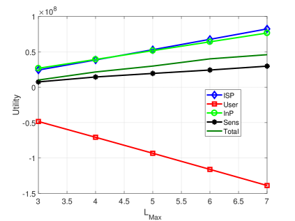
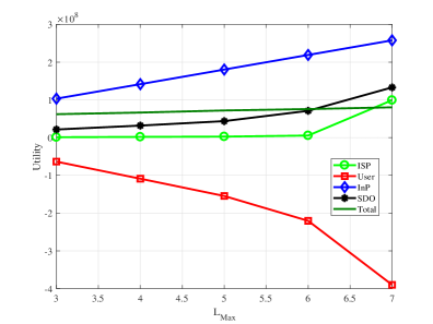
Figure 4: Left:Utility of each player in the max-min approach versus different values of $L_{\text{max}}$. Right: Utility of each player in the weight-one approach versus different values of $L_{\text{max}}$.

Now using the results in the above figures we obtain Figs. 6-Right and 6-Left which depict total revenue and fairness for the max-min, conventional, and weight-one methods.

In general, we look for a setting which has the best total revenue. However, such revenue has to be divided in a fair fashion among the stakeholders. To quantify this fact, we exploit the Jain fairness index [54]. The Jain fairness index for utilities of ISPs, InPs, and SDO is calculated as follows [54]:

$$J(\Phi^{\text{ISP}}_{\text{tot}},\Phi^{\text{InP}}_{\text{tot}},\Phi^{\text{Sens}}_{\text{tot}})=\dfrac{(\Phi^{\text{ISP}}_{\text{tot}}+\Phi^{\text{InP}}_{\text{tot}}+\Phi^{\text{Sens}}_{\text{tot}})^{2}}{3((\Phi^{\text{ISP}}_{\text{tot}})^{2}+(\Phi^{\text{InP}}_{\text{tot}})^{2}+(\Phi^{\text{Sens}}_{\text{tot}})^{2})}.$$ (53)

With the Jain fairness index, when $\Phi^{\text{ISP}}_{\text{tot}}=\Phi^{\text{InP}}_{\text{tot}}=\Phi^{\text{Sens}}_{\text{tot}},$ the best fairness (i.e., $J(\Phi^{\text{ISP}}_{\text{tot}},\Phi^{\text{InP}}_{\text{tot}},\Phi^{\text{Sens}}_{\text{tot}})=1$) is achieved.

As the figures show, if we go with the conventional approach, we are in fact cutting the total revenue. Moreover, the degree of fairness is not also acceptable. By using the weight-one approach, the total revenue is drastically increased. Nevertheless, the resulting fairness is still far from being acceptable. Finally, if we use the max-min approach, we get close to the complete fairness. This is while the total revenue is also increased compared to the conventional approach.

The results prove how the proposed end to end joint pricing and radio resource allocation approach can provide fairness and at the same time, increase the revenue. This is achieved through jointly optimizing the parameters corresponding to all players.

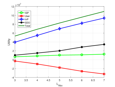
Figure 5: Utility of each player in the conventional approach versus different values of $L_{\text{max}}$.

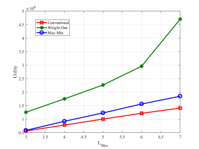
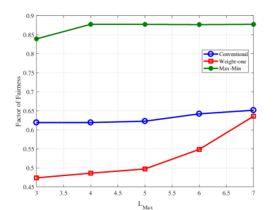
Figure 6: Left:Summation of players utilities for the proposed methods. Right: Fairness index for the proposed methods.

IX Conclusions

In this paper, we provided a novel comprehensive pricing model for IoT services in 5G networks. We considered all the parties involved in the communication scenario and determined the revenue and cost of each party. We formulated the resource allocation in the considered model as a multi-objective optimization problem where in addition to the resource allocation, the pricing variables were also the optimization variables. We solved the resulting problem using the alternating approach and evaluated the performance of the proposed model for different network scenarios using simulations. Moreover, we presented the conventional approach for pricing and radio resource allocation. Simulation results indicate that by applying the proposed joint framework, we can increase the total revenue compared to the conventional case while providing an almost complete fairness among the players. This paves the way to reach the stated goal of the paper: removing one of the barriers that prevent IoT from becoming pervasive.

Appendix A: Suppose that we have a multi-objective maximization problem with objective functions $F$ and $G$, and variable vector $\bm{\varrho}$ formulated as follows:

$$\max_{\bm{\varrho}}\{F(\bm{\varrho}),G(\bm{\varrho})\},\text{s.t.}:\hskip 7.11317ptC_{1}\text{-}C_{K},$$

where $C_{1},\dots,C_{K}$ are the constraints of the optimization problem. In order to solve (IX), one method is scalarization where the original multi-objective problem is transformed into a single objective problem. There are various methods which transform the original problem into a single objective optimization problem. Each single objective optimization problem gives a Pareto optimal solution of the original multi-objective problem. Each of the solutions is determined by a point in the Pareto solution set of the original problem. For example, Fig. 7 shows the Pareto solution set of the maximization problem in which the bold line determines the Pareto boundary. Each of the points can be interpreted as the solution of a specific transformed single objective optimization problem. Suppose that the weighted method is used to transfer the multi-objective into a single objective problem. With the weighted method, the optimization problem (IX) is reformulated as

$$\max_{\bm{\varrho}}WF(\bm{\varrho})+(1-W)G(\bm{\varrho}),\text{s.t.}:\hskip 7.11317ptC_{1}\text{-}C_{K}.$$ (54)

The weighted method is an approach of the scalarization method in which with different values of $W$, various single objective optimization problem can be achieved. When the Pareto solution set is a convex set, such as Fig. 7-Left, with the weighted method all of the points in the Pareto boundary can be achieved. For example, point S1 can be interpreted as a weighted single objective problem in which the weight of function $F$ is $W=1$. Point S2 can be interpreted as a weighted single objective optimization problem in which the main goal is maximizing the fairness between functions $F$ and $G$. Point S3 can be interpreted as a weighted single objective optimization problem in which the weight of function $G$ is $1$ or ($W=0$). As we mentioned, with the weighted approach, all points of the Pareto boundary of a convex Pareto solution set can be achieved. However, finding a value of $W$ which gives the best fairness between $F$ and $G$ is so complicated, while by exploiting the max-min approach as

$$\max_{\bm{\varrho}}\{\min_{F,G}\{F(\bm{\varrho}),G(\bm{\varrho})\}\},\text{s.t.}:\hskip 7.11317ptC_{1}\text{-}C_{K},$$ (55)

the best fairness can be easily achieved. Moreover, if the Pareto solution set not be a convex set, such as Fig. 7-Right, the weighted approach can not achieve all of the Pareto boundary points. For example, in Fig. 7-Right, point S2 (consider that S2 gives the best fairness) can not be achieved with the weighted approach. In this case, the max-min method can be applied to achieve the best fairness between $F$ and $G$. From the above explanation, we can find that in a multi-objective optimization problem, considering the main goal of the multi-objective optimization problem, a single objective optimization problem can be formulated from the main multi-objective problem. It should be noted that, in addition to the main goal of the transformed optimization problem, its solution complexity can have essential role in selecting the form of the transformed optimization problem. The proposed max-min approach comes from this fact that the fairness among ISPs, SDO and InPs has the maximum values, and also, the utility function of users has the maximum value. It should be noted that, due to the this fact that the user utility has a negative value, it is not possible to consider it as an entry of the max-min approach.

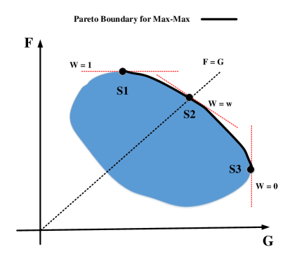
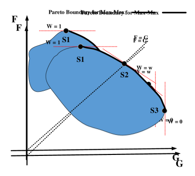
Figure 7: Left:Convex Pareto boundary of a multi-objective maximization problem with two objective functions. Right: Non-convex Pareto boundary of a multi-objective maximization problem with two objective functions.

References

- [1] A. Kamilaris and A. Pitsillides, “Mobile phone computing and the internet of things: A survey,” IEEE Internet of Things Journal, vol. 3, no. 6, pp. 885–898, Dec 2016.
- [2] S. Vashi, J. Ram, J. Modi, S. Verma, and C. Prakash, “in proc. internet of things (IoT): A vision, architectural elements, and security issues,” in 2017 International Conference on I-SMAC (IoT in Social, Mobile, Analytics and Cloud) (I-SMAC), Feb 2017, pp. 492–496.
- [3] C. Liang and F. R. Yu, “Wireless network virtualization: A survey, some research issues and challenges,” IEEE Communications Surveys Tutorials, vol. 17, no. 1, pp. 358–380, Firstquarter 2015.
- [4] D. Niyato, D. T. Hoang, N. C. Luong, P. Wang, D. I. Kim, and Z. Han, “Smart data pricing models for the internet of things: a bundling strategy approach,” IEEE Network, vol. 30, no. 2, pp. 18–25, Mar 2016.
- [5] D. Niyato, M. A. Alsheikh, P. Wang, D. I. Kim, and Z. Han, “Market model and optimal pricing scheme of big data and internet of things (IoT),” in Proc 2016 IEEE International Conference on Communications (ICC), May 2016, pp. 1–6.
- [6] J. Denis, M. Pischella, and D. L. Ruyet, “Energy-efficiency-based resource allocation framework for cognitive radio networks with fbmc/ofdm,” IEEE Transactions on Vehicular Technology, vol. 66, no. 6, pp. 4997–5013, Jun. 2017.
- [7] A. Sultana, L. Zhao, and X. Fernando, “Efficient resource allocation in device-to-device communication using cognitive radio technology,” IEEE Transactions on Vehicular Technology, vol. 66, no. 11, pp. 10 024–10 034, Nov 2017.
- [8] D. T. Ngo, S. Khakurel, and T. Le-Ngoc, “Joint subchannel assignment and power allocation for OFDMA femtocell networks,” IEEE Transactions on Wireless Communications, vol. 13, no. 1, pp. 342–355, Jan. 2014.
- [9] J. Li, Q. Sun, and G. Fan, “Resource allocation for multiclass service in IoT uplink communications,” in Proc. 2016 3rd International Conference on Systems and Informatics (ICSAI), Nov 2016, pp. 777–781.
- [10] H. Kebriaei, B. Maham, and D. Niyato, “Bandwidth price optimization for D2D communications underlaying cellular networks,” in Proc. IEEE WCNC’14, Apr. 2014, pp. 1608–1614.
- [11] P. Li, S. Guo, and I. Stojmenovic, “A truthful double auction for device-to-device communications in cellular networks,” IEEE Journal on Selected Areas in Communications, vol. 34, no. 1, pp. 71–81, Jan. 2016.
- [12] C. Xu, L. Song, Z. Han, D. Li, and B. Jiao, “Resource allocation using a reverse iterative combinatorial auction for device-to-device underlay cellular networks,” in Proc. IEEE GLOBECOM’12, Dec. 2012, pp. 4542–4547.
- [13] C. Xu, L. Song, Z. Han, Q. Zhao, X. Wang, and B. Jiao, “Interference-aware resource allocation for device-to-device communications as an underlay using sequential second price auction,” in Proc. IEEE ICC, 2012, pp. 445–449.
- [14] C. Jiang, Y. Chen, K. R. Liu, and Y. Ren, “Network economics in cognitive networks,” IEEE Communications Magazine, vol. 53, no. 5, pp. 75–81, May 2015.
- [15] Y. Xing, R. Chandramouli, and C. Cordeiro, “Price dynamics in competitive agile spectrum access markets,” IEEE Journal on Selected Areas in Communications, vol. 25, no. 3, pp. 613–621, Apr. 2007.
- [16] O. Ileri, D. Samardzija, T. Sizer, and N. B. Mandayam, “Demand responsive pricing and competitive spectrum allocation via a spectrum server,” in Proc. IEEE DySPAN’05, Nov. 2005, pp. 194–202.
- [17] D. Niyato and E. Hossain, “Competitive pricing for spectrum sharing in cognitive radio networks: Dynamic game, inefficiency of nash equilibrium, and collusion,” IEEE Journal on Selected Areas in Communications, vol. 26, no. 1, pp. 192–202, Jan. 2008.
- [18] S. Gandhi, C. Buragohain, L. Cao, H. Zheng, and S. Suri, “A general framework for wireless spectrum auctions,” in Proc. IEEE DySPAN’07, Apr. 2007, pp. 22–33.
- [19] D. Niyato and E. Hossain, “Hierarchical spectrum sharing in cognitive radio: A microeconomic approach,” in Proc. IEEE WCNC’07, Mar. 2007, pp. 3822–3826.
- [20] O. Simeone, I. Stanojev, S. Savazzi, Y. Bar-Ness, U. Spagnolini, and R. Pickholtz, “Spectrum leasing to cooperating secondary ad hoc networks,” IEEE Journal on Selected Areas in Communications, vol. 26, no. 1, pp. 203–213, Jan. 2008.
- [21] D. Niyato and E. Hossain, “Market equilibrium, competitive, and cooperative pricing for spectrum sharing in cognitive radio networks: analysis and comparison,” IEEE Transactions on Wireless Communications, vol. 7, no. 11, pp. 4273–4283, Nov. 2008.
- [22] H. Sartono, Y. H. Chew, W. H. Chin, and C. Yuen, “Joint demand and supply auction pricing strategy in dynamic spectrum sharing,” in Proc. IEEE PIMRC, Sep. 2009, pp. 833–837.
- [23] C. Jiang, Y. Chen, K. R. Liu, and Y. Ren, “Optimal pricing strategy for operators in cognitive femtocell networks,” IEEE Transactions on Wireless Communications, vol. 13, no. 9, pp. 5288–5301, Sep. 2014.
- [24] D. Niyato and E. Hossain, “Wireless broadband access: WiMax and beyond-integration of WiMax and WiFi: Optimal pricing for bandwidth sharing,” IEEE Communications Magazine, vol. 45, no. 5, pp. 140–146, May 2007.
- [25] S.-Y. Yun, Y. Yi, D.-H. Cho, and J. Mo, “The economic effects of sharing femtocells,” IEEE Journal on Selected Areas in Communications, vol. 30, no. 3, pp. 595–606, Apr. 2012.
- [26] X. Kang, R. Zhang, and M. Motani, “Price-based resource allocation for spectrum-sharing femtocell networks: A stackelberg game approach,” IEEE Journal on Selected Areas in Communications, vol. 30, no. 3, pp. 538–549, Apr. 2012.
- [27] N. Shetty, S. Parekh, and J. Walrand, “Economics of femtocells,” in Proc. IEEE GLOBECOM’09, Dec. 2009, pp. 1–6.
- [28] L. Duan, J. Huang, and B. Shou, “Economics of femtocell service provision,” IEEE Transactions on Mobile Computing, vol. 12, no. 11, pp. 2261–2273, Nov. 2013.
- [29] Y. Yi, J. Zhang, Q. Zhang, and T. Jiang, “Spectrum leasing to femto service provider with hybrid access,” in Proc. IEEE INFOCOM’12, Mar. 2012, pp. 1215–1223.
- [30] Y. Chen, J. Zhang, and Q. Zhang, “Utility-aware refunding framework for hybrid access femtocell network,” IEEE Transactions on Wireless Communications, vol. 11, no. 5, pp. 1688–1697, May 2012.
- [31] K. Zhu, E. Hossain, and D. Niyato, “Pricing, spectrum sharing, and service selection in two-tier small cell networks: A hierarchical dynamic game approach,” IEEE Transactions on Mobile Computing, vol. 13, no. 8, pp. 1843–1856, Aug. 2014.
- [32] J. Wang, C. Jiang, Z. Bie, T. Q. Quek, and Y. Ren, “Mobile data transactions in device-to-device communication networks: pricing and auction,” IEEE Communications Letters, vol. 5, no. 3, pp. 300–303, Jun. 2016.
- [33] Q. Xu, Y. Chen, and K. J. R. Liu, “Optimal pricing for interference control in time-reversal device-to-device uplinks,” in Proc. IEEE GlobalSIP, 2015, pp. 1096–1100.
- [34] D. Yang, X. Fang, and G. Xue, “Truthful auction for cooperative communications,” in Proc. ACM International Symposium on Mobile Ad Hoc Networking and Computing, 2011, pp. 1–10.
- [35] D. Niyato, D. T. Hoang, N. C. Luong, P. Wang, D. I. Kim, and Z. Han, “Smart data pricing models for the internet of things: a bundling strategy approach,” IEEE Network, vol. 30, no. 2, pp. 18–25, Apr.-Mar. 2016.
- [36] D. Niyato, M. A. Alsheikh, P. Wang, D. I. Kim, and Z. Han, “Market model and optimal pricing scheme of big data and internet of things (IoT),” arXiv preprint arXiv:1602.03202, 2016.
- [37] D. Niyato, P. Wang, and D. I. Kim, “Optimal service auction for wireless powered internet of things (IoT) device,” in Proc IEEE GLOBECOM’15, 2015, pp. 1–6.
- [38] A. E. Al-Fagih, F. M. Al-Turjman, W. M. Alsalih, and H. S. Hassanein, “A priced public sensing framework for heterogeneous IoT architectures,” IEEE Transactions on Emerging Topics in Computing, vol. 1, no. 1, pp. 133–147, Jun. 2013.
- [39] M. J. Farooq and Q. Zhu, “Adaptive and resilient revenue maximizing dynamic resource allocation and pricing for cloud-enabled iot systems,” arXiv preprint arXiv:1707.08691v3, 2018.
- [40] A. Kiani and N. Ansari, “Towards hierarchical mobile edge computing: An auction-based profit maximization approach,” IEEE Internet of Things Journal, vol. 4, pp. 2082–2091, Dec.2 017.
- [41] H. Zhang, Y. Xiao, S. Bu, D. Niyato, F. R. Yu, and Z. Han, “Computing resource allocation in three-tier IoT Fog networks: A joint optimization approach combining stackelberg game and matching,” IEEE Internet of Things Journal, vol. 4, no. 5, pp. 1204–1215, Oct 2017.
- [42] H. Nikopour and H. Baligh, “Sparse code multiple access,” in Proc. 2013 IEEE 24th Annual International Symposium on Personal, Indoor, and Mobile Radio Communications (PIMRC), Sept 2013, pp. 332–336.
- [43] S. Zhang, X. Xu, L. Lu, Y. Wu, G. He, and Y. Chen, “Sparse code multiple access: An energy efficient uplink approach for 5G wireless systems,” in Proc. 2014 IEEE Global Communications Conference, Dec 2014, pp. 4782–4787.
- [44] M. Moltafet, N. M. Yamchi, M. R. Javan, and P. Azmi, “Comparison study between PD-NOMA and SCMA,” IEEE Transactions on Vehicular Technology, vol. 67, no. 2, pp. 1830–1834, Feb 2018.
- [45] J. H. Cho, Y. Wang, I. R. Chen, K. S. Chan, and A. Swami, “A survey on modeling and optimizing multi-objective systems,” IEEE Communications Surveys Tutorials, vol. 19, no. 3, pp. 1867–1901, thirdquarter 2017.
- [46] K. Deb, “Solving goal programming problems using multi-objective genetic algorithms,” in Proc. Congress on Evolutionary Computation-CEC99 (Cat. No. 99TH8406), vol. 1, 1999, p. 84 Vol. 1.
- [47] E. Bjornson, E. A. Jorswieck, M. Debbah, and B. Ottersten, “Multiobjective signal processing optimization: The way to balance conflicting metrics in 5G systems,” IEEE Signal Processing Magazine, vol. 31, no. 6, pp. 14–23, Nov 2014.
- [48] R. Hooke and T. A. Jeeves, “Direct search solution of numerical and statistical problems,” Journal of the ACM (JACM), vol. 8, no. 2, pp. 212–229, 1961.
- [49] I. C. Research, “CVX: Matlab software for disciplined convex programming,” http://cvxr.com/cvx, Aug 2012.
- [50] A. Zappone, E. Björnson, L. Sanguinetti, and E. Jorswieck, “A framework for globally optimal energy-efficient resource allocation in wireless networks,” in 2016 IEEE International Conference on Acoustics, Speech and Signal Processing (ICASSP), March 2016, pp. 3616–3620.
- [51] ——, “Globally optimal energy-efficient power control and receiver design in wireless networks,” IEEE Transactions on Signal Processing, vol. 65, no. 11, pp. 2844–2859, June 2017.
- [52] L. Venturino, N. Prasad, and X. Wang, “Coordinated scheduling and power allocation in downlink multicell OFDMA networks,” IEEE Transactions on Vehicular Technology, vol. 58, no. 6, pp. 2835–2848, July 2009.
- [53] R. C. de Lamare and R. Sampaio-Neto, “Adaptive reduced-rank equalization algorithms based on alternating optimization design techniques for mimo systems,” IEEE Transactions on Vehicular Technology, vol. 60, no. 6, pp. 2482–2494, July 2011.
- [54] A. B. Sediq, R. H. Gohary, R. Schoenen, and H. Yanikomeroglu, “Optimal tradeoff between sum-rate efficiency and jain’s fairness index in resource allocation,” IEEE Transactions on Wireless Communications, vol. 12, no. 7, pp. 3496–3509, July 2013.