Chiral spin ordering of electron gas in solids with broken time reversal symmetry
K. S. Denisov
denisokonstantin@gmail.comIoffe Institute, 194021 St.Petersburg, Russia
Lappeenranta-Lahti University of Technology, FI-53851 Lappeenranta, Finland
I. V. Rozhansky
Ioffe Institute, 194021 St.Petersburg, Russia
Lappeenranta-Lahti University of Technology, FI-53851 Lappeenranta, Finland
N. S. Averkiev
Ioffe Institute, 194021 St.Petersburg, Russia
E. Lähderanta
Lappeenranta-Lahti University of Technology, FI-53851 Lappeenranta, Finland
Abstract
In this work we manifest that an electrostatic disorder
in conducting systems with broken time reversal symmetry universally leads to a chiral ordering of the electron gas
giving rise to skyrmion-like textures in spatial distribution of the electron spin density.
We describe a microscopic mechanism underlying the formation of the equilibrium chiral spin textures
in two-dimensional systems with
spin-orbit interaction and exchange spin splitting. We have obtained analytical expressions for spin-density response functions and have analyzed both local and non-local spin response to electrostatic perturbations for systems
with parabolic-like and Dirac electron spectra.
With the proposed theory we come up with a concept of
controlling spin chirality by electrical means.
The concept of spin chirality constitutes a substantial part of modern condensed matter physics.
It is widely applied for strongly correlated electron systems Wen et al. (1989); Chen et al. (2010a); Batista et al. (2016); Kallin and Berlinsky (2016) when interpreting
the fractional statistics Kalmeyer and Laughlin (1987); Yang et al. (1993); Kitaev (2006), or chiral spin liquids Volovik (2016); Lee and Nagaosa (1992); Bauer et al. (2014); Messio et al. (2017) in terms of an effective gauge field.
Remarkably, a finite spin chirality
induces a gauge invariant magnetic flux, which is an experimentally observable quantity Wen et al. (1989).
It was shown that the chirality driven magnetic field
affects electron transport in the very same way as the ordinary magnetic field does Ye et al. (1999); Chun et al. (2000) leading to the Hall response,
the phenomenon currently referred as the topological Hall effect Bruno et al. (2004); Denisov et al. (2018); Hamamoto et al. (2015).
Naturally, to get an experimental access to the variety of spin chirality driven phenomena an efficient tool for creating chiral spin ordrer is needed.
One way towards this goal is to focus on materials
possessing exotic spin textures, such as magnetic skyrmions Fert et al. (2017); Wiesendanger (2016); Soumyanarayanan
et al. (2017); Nakajima et al. (2017), or merons Yu et al. (2018).
Still, exploring the physical mechanisms behind the emergence of spin chirality in solids remains challenging and is of high fundamental interest.
In this Letter we show that in systems with broken time reversal symmetry (-symmetry)
a chiral spin order of electron gas is universally induced by an electrostatic disorder,
which is an inherent property of any real solid.
We argue that
numerous crystal imperfections, such as
residue impurities or surface defects
appear to be a source of local chiral spin ordering in the electron gas.
This effect is more pronounced for an electron gas with stronger spin-orbit interaction (SOI).
Naturally, various magnetic
systems
such as magnetic topological insulators (TI) Tokura et al. (2019); Okada et al. (2011); Wei et al. (2013); Chen et al. (2010b),
Rashba magnetic layers Miron et al. (2010, 2011); Manchon et al. (2015); Zhou et al. (2018) or dilute magnetic semiconductors (DMS) Liu et al. (2008); Yu et al. (2010); Chernyshov et al. (2009); Novik et al. (2005); Jungwirth et al. (2014); Li et al. (2013)
are in fact flooded by chiral spin textures pinned to structural defects.
This effect opens up
a novel concept of an experimental research of spin chirality
driven phenomena.
In our work we focus on
two-dimensional degenerate electron gas (2DEG) with
a spin-orbit interaction and an exchange spin splitting.
We introduce an effective ’magnetic field’ acting on an electron spin:
(1)
where
is a 2D momentum with magnitude and polar angle .
The parameter describes the out-of-plane component leading to the carrier spin splitting at ,
it is thus responsible for the violation of -symmetry.
The in-plane components of represent linear in terms due to SOI, is the SOI coupling constant.
The SOI parameters (helicity) and (vorticity)
cover different types of the SOI interaction.
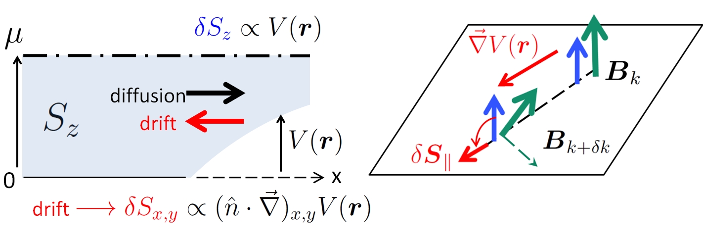
Figure 1: The physical picture behind the emergence of an equilibrium chiral spin pattern of the electron gas. The in-plane spin arises from the precession due to drift electron flow.
Let us further assume an electrostatic disorder due to various defects
present in the system.
When -symmetry is broken the
spatial distribution of the equilibrium electron spin density
follows the inhomogeneity of the electrostatic potential .
Indeed, at there is a nonzero electron spin polarization directed perpendicular to the motion plane (-axis).
A local shift of
leads to a spatial redistribution of electrons and, hence, to the change of . When SOI is present ()
the in-plane components of the spin density appear as well, so
the induced spin response acquires a chiral spatial pattern forming skyrmion-like spin textures.
Let us notice that the
mechanics behind the appearance of
in response to an electrostatic potential
has a peculiar character,
and it differs
from that for .
Since there is no net in-plane spin polarization at a spatially uniform electrostatic potential, appears only due to its gradient. One can consider the following quaisclassical picture, see Fig.1.
An electron with initial momentum and spin co-aligned
with the direction of
moves along a certain trajectory.
Due to the electrostatic potential
gradient
the carrier momentum is changed ,
thus changing the tilt of the magnetic field ,
which in-plane components are coupled with momentum.
This process triggers the precession of electron spin
around the new direction of the magnetic field
creating an excessive in-plane spin density.
In the thermodynamic equilibrium there is no net current
as the drift and diffusion electron flows are compensated everywhere.
However, the in-plane components of the spin density still appear
because the drift flow is associated with a change of the electron momentum.
The emergence of the spin textures due to spatial variation of the electrostatic
potential is described by static spin-density response functions:
(2)
where
is a spin operator for axis,
index denotes
two electron subbands,
and are the energy and the Bloch amplitude of an electron in state ,
is the equilibrium distribution function.
Using the functions one can analyze
the spin density emerging in 2DEG in the
vicinity of a doping center or a defect characterized by a
potential :
(3)
where is the Fourier transform of , the electron-electron interaction is neglected.
In particular, the functions
allow us to identify whether the spin response is local or
extends beyond the localization radius of the potential
due to the wave properties of 2DEG.
Let us point out a few general features
of the spin response in the considered model.
As has been mentioned above,
-component of spin is analogous to the electron density, so
if there is no spatial dispersion
locally couples with the potential
.
The coefficient is given by
a product of the electron density of states and -projection of spin taken at the Fermi energy. On the contrary, the in-plane spin components driven by the precession mechanism illustrated by Fig. 1 are induced by the gradient of .
In the case of a local response this coupling takes the form
,
where is a unitary matrix determined by SOI type,
and the coefficient is determined by a carrier spectrum. Since the Fourier transform of is , we conclude
that are purely imaginary,
we present them as
(4)
where the real function depends on the absolute value of ,
.
Naturally,
at .
As soon as there is some spatial inhomogeneity of crystalline structure the electron gas acquires a local spin chirality.
For an axially symmetric potential
the excessive
spin density
profile has a shape:
(5)
where are the polar coordinates of a radius vector,
depend on , are Bessel’s functions of the zeroth and first order, respectively, .
The emerging chiral spin cloud is similar to a skyrmion for , or to an antiskyrmion for .
The fact that the helicity of the real space spin rotation is shifted by with respect to in -space
reflects the
spin precession mechanism.
The details of chiral spin response naturally depend on a carrier band structure .
Below we calculate , which is a sum of the responses of two subbands (see Supplementary materials), and
analyze the spin response for parabolic-like and Dirac electron spectra.
Parabolic-like spectrum.
Let us assume the following Hamiltonian and the energy spectrum :
(6)
where is the effective mass in the absence of the field (we assume =1).
In this paper we take the parameter .
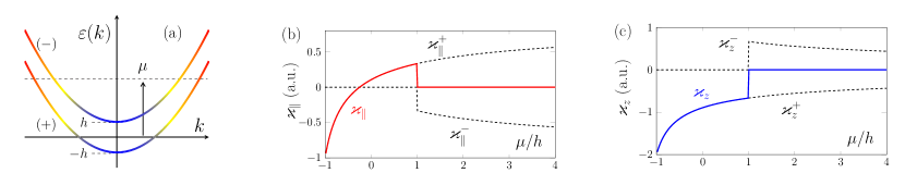
The spectrum of the system is shown in Fig. 2a, the color within each subband indicates
the magnitude of , which has a meaning of
spin inclination into the plane of the carrier motion
(blue color corresponds to , red color
indicates ).
We have obtained analytic expressions for the spin-density response functions with the spectrum given by Eq. 6.
As the formulas are rather cumbersome, we provide them in the Supplementary Materials.
Importantly, within each subband are decomposed onto a sum of intra- and interband contributions
with the interband terms exhibiting an additional coupling .
Let us firstly consider the local coupling regime, when
and
.
The coefficients
found from the limiting behavior of at
are given in Supplementary Materials.
As already mentioned, is
the product of the density of states
and the spin -projection at the Fermi energy .
The dependence of on is shown in Fig 2b,c.
We note that nonzero spin response is observed only when
the upper subband is free of electrons (). This result is an inherent property of the considered model; the
background spin density remains constant at .
As follows from the
explicit expressions for ,
the local coupling regime occurs
when the Fourier components of are localized within
, where .
For these values the response functions ,
have a weak dependence on , which
means no spatial dispersion and, thus, the absence of non-locality in the response.
Note, that, apart from the Fermi wavevector ,
there is a second spatial scale , which
controls the spatial dispersion of the spin response.
This scale is associated with the precession
mechanism for the in-plane spin generation.
Naturally, a more interesting spin physics takes place when the effects of spatial dispersion come to the fore.
We first consider the case when only the subband is populated ().
The dependence of , and its partial contributions on
are shown in Fig. 3(a,b).
As we have discussed above, the response functions at behave as
,
.
Another general trend is that the intra- and interband terms
have an opposite sign and, thus, tend to cancel each other.
The spatial profile
induced around a repulsive short range potential is shown in Fig. 3c.
The largest spin response appears
within the Fermi wavelength ().
Going away from the center decrease exhibiting the Friedel oscillations with the period (see inset in Fig.3).
Let us now consider the case when both spin subbands are populated.
Although the local spin response is absent in this case (,
the effect of spatial dispersion restores a chiral spin pattern.
Shown in Fig. 3(d-g) are the calculated spin response functions .
We note that the intraband terms
for both subbands exhibit a single spike at .
What is more interesting is the double-spike structure of the interband terms
driven by
two nesting vectors connecting two distinct subbands of the Fermi surface.
The presence of the two different spatial scales along with a complex structure of interband transitions
lead to quite a peculiar spin response in the real space.
In Fig. 3h,i we demonstrate
for the short range potential .
The spatial scale is given in units of , where is the averaged Fermi wavevector.
The Friedel oscillations clearly visible at large distances from the centre
are now formed by the superposition of oscillations with different spatial periods.
Dirac spectrum.
Let us further consider the case of Hamiltonian with Dirac spectrum:
(7)
This model describes, for example,
chiral surface states of a 3D TI (the SOI parameters are , ).
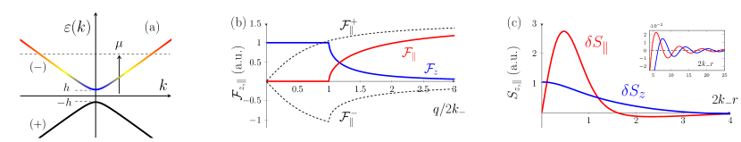
Shown in Fig. 4a is the spectrum (7), which consists of two
nearly linear bands separated by the gap .
The fundamental difference
from the previously considered parabolic-like spectrum
is the additional electron-hole symmetry (-symmetry),
which modifies the electron gas response to external perturbations
Hwang and Das Sarma (2007); Wunsch et al. (2006); Zhu et al. (2011); Checkelsky et al. (2012).
Let us put the Fermi energy above the charge neutrality point,
so the lower band is completely filled while the upper band is filled partially.
Our calculations show that
the fillled lower subband does not contribute to the response of spin component (),
while for the upper subband
the spin response function
is the conventional 2D Lindhard function:
(8)
where is an effective mass due to the spectrum gap,
is the Fermi wavevector.
This result is rather interesting as
the Lindhard function usually describes the susceptibility of a system with simple parabolic spectrum.
Another important feature of given by (8) is that
its magnitude does not depend on the Fermi energy .
This is in contrast with
the parabolic-like case, where the increase of leads to the suppression of spin response according to at .
This effect is due to
the density of states, which for the Dirac spectrum takes the form .
Upon the increase of the Fermi energy the suppression of spin -projection (which is at )
is exacltly compensated by the increase of . For instance, considering the local coupling regime
the spin response is explicitly determined by a product independent of .
The in-plane spin response also exhibits a number of peculiar features.
For the functions we obtained:
(9)
We note that there is a non-zero spin response from the completely filled subband, and that remains finite
even at .
This is an unusual behavior, since no density response of subband can be induced in this case.
Indeed, the interband transitions underlying the change of electron density are suppressed for a smooth potential
due to the finite band gap .
On the contrary, the in-plane spin response originates from the spin precession driven by a drift electron flow, which
remains finite in -symmetry systems even with gaped spectrum due to the Klein tunneling.
Considering the in-plane spin response from the upper subband we note that
the function given by Eq. 9
contains both the -independent term opposite to that of subband,
and a -aware contribution responsible for the Friedel’s oscillations with the spatial period .
The in-plane spin response function and its partial components
are shown in Fig. 4b.
The contributions of subbands cancel each other at and turns to zero.
Therefore, no in-plane spin response is induced by a long-range electrostatic perturbation
when the Fermi level is in the upper subband.
The non-local spin response is also modified due to -symmetry.
As can be seen in Fig. 4b the function
saturates at instead of going to zero.
However, as discussed above, the in-plane spin density responds
to the potential gradient, so it is
which has the physical meaning and it indeed decays as when
saturates.
In Fig. 4c we show
the spatial spin pattern induced by a short-range potential , is a potential radius.
It is worth mentioning that the magnitude of the in-plane spin response in the vicinity of a defect is far larger than in the
parabolic spectra case due to the saturation of .
This finding emphasizes a particularly high susceptibility of chiral spin pattern in response to an electrostatic disorder in systems with Dirac spectrum.
Discussion.
Our study suggests that the emergence of chiral spin textures
driven by an electrostatic disorder is a universal phenomena.
The obtained results are applicable
to a variety of
experimentally studied systems, such as DMS Gaj and Kossut (2010); Jungwirth et al. (2014), thin films of
ferromagnets Miron et al. (2010, 2011),
Bi2Se3 doped by magnetic impurities Wei et al. (2013); Chen et al. (2010b); Kou et al. (2012); Watson et al. (2013),
or due to the proximity effect Žutić
et al. (2018) with magnetic insulators Vobornik et al. (2011), or ferromagnets Lv et al. (2018); Lee et al. (2018).
We note, that the chiral perturbation of the electron spin density
manifests itself in various ways.
For instance, probing the chiral spin textures induced on
a surface
by means of spin-polarized scanning tunneling microscopy Wiesendanger (2009) would be a new tool
to access the parameters of the electron gas.
The chiral spin pattern
in the electron gas can also induce a chiral
order of magnetic ions located either in the same material or
in a different layer of a heterostructure due to proximity effect.
Therefore, the phenomenon opens a way to record the information using magnetic skyrmions or similar chiral spin textures by electrical means.
Finally, the topological Hall effect is
generally expected in
magnetic systems with spin-orbit interaction due to asymmetric scattering of electrons on chiral spin textures Denisov et al. (2018) pinned to defects and other inhomogeneities.
In particular, the considered mechanism could be responsible for the recently observed topological Hall effect in TI and DMS Jiang et al. (2019); Liu et al. (2017); Oveshnikov et al. (2015).
The work has been supported by the Russian Science Foundation
(Project 18-72-10111), the Russian Foundation of Basic Research (grant 18-02-00668), and
the Academy of Finland (Grant No. 318500).
K.S.D. and N.S.A. thank the Foundation for the Advancement of Theoretical Physics and
Mathematics “BASIS”.
References
Wen et al. (1989)
X. G. Wen,
F. Wilczek, and
A. Zee,
Phys. Rev. B 39,
11413 (1989).
Chen et al. (2010a)
X. Chen,
Z.-C. Gu, and
X.-G. Wen,
Physical review b 82,
155138 (2010a).
Batista et al. (2016)
C. D. Batista,
S.-Z. Lin,
S. Hayami, and
Y. Kamiya,
Reports on Progress in Physics
79, 084504
(2016).
Kallin and Berlinsky (2016)
C. Kallin and
J. Berlinsky,
Reports on Progress in Physics
79, 054502
(2016).
Kalmeyer and Laughlin (1987)
V. Kalmeyer and
R. B. Laughlin,
Phys. Rev. Lett. 59,
2095 (1987).
Yang et al. (1993)
K. Yang,
L. Warman, and
S. Girvin,
Physical review letters 70,
2641 (1993).
Kitaev (2006)
A. Kitaev,
Annals of Physics 321,
2 (2006).
Volovik (2016)
G. Volovik,
JETP lett 103,
140 (2016).
Lee and Nagaosa (1992)
P. A. Lee and
N. Nagaosa,
Physical Review B 46,
5621 (1992).
Bauer et al. (2014)
B. Bauer,
L. Cincio,
B. P. Keller,
M. Dolfi,
G. Vidal,
S. Trebst, and
A. W. Ludwig,
Nature communications 5,
5137 (2014).
Messio et al. (2017)
L. Messio,
S. Bieri,
C. Lhuillier,
and B. Bernu,
Phys. Rev. Lett. 118,
267201 (2017).
Ye et al. (1999)
J. Ye,
Y. B. Kim,
A. J. Millis,
B. I. Shraiman,
P. Majumdar, and
Z. Tešanović, Phys.
Rev. Lett. 83, 3737
(1999).
Chun et al. (2000)
S. Chun,
M. Salamon,
Y. Lyanda-Geller,
P. Goldbart, and
P. Han,
Physical review letters 84,
757 (2000).
Bruno et al. (2004)
P. Bruno,
V. K. Dugaev,
and
M. Taillefumier,
Phys. Rev. Lett. 93,
096806 (2004).
Denisov et al. (2018)
K. Denisov,
I. Rozhansky,
N. Averkiev, and
E. Lähderanta,
Physical Review B 98,
195439 (2018).
Hamamoto et al. (2015)
K. Hamamoto,
M. Ezawa, and
N. Nagaosa,
Phys. Rev. B 92,
115417 (2015).
Fert et al. (2017)
A. Fert,
N. Reyren, and
V. Cros,
Nature Reviews Materials 2,
17031 (2017).
Wiesendanger (2016)
R. Wiesendanger,
Nature Reviews Materials 1,
16044 (2016).
Soumyanarayanan
et al. (2017)
A. Soumyanarayanan,
M. Raju,
A. G. Oyarce,
A. K. Tan,
M.-Y. Im,
A. P. Petrović,
P. Ho,
K. Khoo,
M. Tran,
C. Gan, et al.,
Nature materials 16,
898 (2017).
Nakajima et al. (2017)
T. Nakajima,
H. Oike,
A. Kikkawa,
E. P. Gilbert,
N. Booth,
K. Kakurai,
Y. Taguchi,
Y. Tokura,
F. Kagawa, and
T.-h. Arima,
Science advances 3,
e1602562 (2017).
Yu et al. (2018)
X. Yu,
W. Koshibae,
Y. Tokunaga,
K. Shibata,
Y. Taguchi,
N. Nagaosa, and
Y. Tokura,
Nature 564, 95
(2018).
Tokura et al. (2019)
Y. Tokura,
K. Yasuda, and
A. Tsukazaki,
Nature Reviews Physics 1,
126 (2019).
Okada et al. (2011)
Y. Okada,
C. Dhital,
W. Zhou,
E. D. Huemiller,
H. Lin,
S. Basak,
A. Bansil,
Y.-B. Huang,
H. Ding,
Z. Wang, et al.,
Phys. Rev. Lett. 106,
206805 (2011).
Wei et al. (2013)
P. Wei,
F. Katmis,
B. A. Assaf,
H. Steinberg,
P. Jarillo-Herrero,
D. Heiman, and
J. S. Moodera,
Phys. Rev. Lett. 110,
186807 (2013).
Chen et al. (2010b)
Y. Chen,
J.-H. Chu,
J. Analytis,
Z. Liu,
K. Igarashi,
H.-H. Kuo,
X. Qi,
S.-K. Mo,
R. Moore,
D. Lu, et al.,
Science 329,
659 (2010b).
Miron et al. (2010)
I. M. Miron,
G. Gaudin,
S. Auffret,
B. Rodmacq,
A. Schuhl,
S. Pizzini,
J. Vogel, and
P. Gambardella,
Nature materials 9,
230 (2010).
Miron et al. (2011)
I. M. Miron,
K. Garello,
G. Gaudin,
P.-J. Zermatten,
M. V. Costache,
S. Auffret,
S. Bandiera,
B. Rodmacq,
A. Schuhl, and
P. Gambardella,
Nature 476,
189 (2011).
Manchon et al. (2015)
A. Manchon,
H. C. Koo,
J. Nitta,
S. Frolov, and
R. Duine,
Nature materials 14,
871 (2015).
Zhou et al. (2018)
L. Zhou,
H. Song,
K. Liu,
Z. Luan,
P. Wang,
L. Sun,
S. Jiang,
H. Xiang,
Y. Chen,
J. Du, et al.,
Science advances 4,
eaao3318 (2018).
Liu et al. (2008)
C.-X. Liu,
X.-L. Qi,
X. Dai,
Z. Fang, and
S.-C. Zhang,
Physical review letters 101,
146802 (2008).
Yu et al. (2010)
R. Yu,
W. Zhang,
H.-J. Zhang,
S.-C. Zhang,
X. Dai, and
Z. Fang,
Science 329,
61 (2010).
Chernyshov et al. (2009)
A. Chernyshov,
M. Overby,
X. Liu,
J. K. Furdyna,
Y. Lyanda-Geller,
and L. P.
Rokhinson, Nature Physics
5, 656 (2009).
Novik et al. (2005)
E. Novik,
A. Pfeuffer-Jeschke,
T. Jungwirth,
V. Latussek,
C. Becker,
G. Landwehr,
H. Buhmann, and
L. Molenkamp,
Physical Review B 72,
035321 (2005).
Jungwirth et al. (2014)
T. Jungwirth,
J. Wunderlich,
V. Novák,
K. Olejnik,
B. Gallagher,
R. Campion,
K. Edmonds,
A. Rushforth,
A. Ferguson, and
P. Němec,
Reviews of Modern Physics 86,
855 (2014).
Li et al. (2013)
H. Li,
X. Wang,
F. Doǧan, and
A. Manchon,
Applied Physics Letters 102,
192411 (2013).
Hwang and Das Sarma (2007)
E. H. Hwang and
S. Das Sarma,
Phys. Rev. B 75,
205418 (2007).
Wunsch et al. (2006)
B. Wunsch,
T. Stauber,
F. Sols, and
F. Guinea,
New Journal of Physics 8,
318 (2006).
Zhu et al. (2011)
J.-J. Zhu,
D.-X. Yao,
S.-C. Zhang, and
K. Chang,
Phys. Rev. Lett. 106,
097201 (2011).
Checkelsky et al. (2012)
J. G. Checkelsky,
J. Ye,
Y. Onose,
Y. Iwasa, and
Y. Tokura,
Nature Physics 8,
729 (2012).
Gaj and Kossut (2010)
J. A. Gaj and
J. Kossut,
144, 27 (2010).
Kou et al. (2012)
X. Kou,
W. Jiang,
M. Lang,
F. Xiu,
L. He,
Y. Wang,
Y. Wang,
X. Yu,
A. Fedorov,
P. Zhang,
et al., Journal of Applied Physics
112, 063912
(2012).
Watson et al. (2013)
M. Watson,
L. Collins-McIntyre,
L. Shelford,
A. I. Coldea,
D. Prabhakaran,
S. Speller,
T. Mousavi,
C. R. M. Grovenor,
Z. Salman,
S. Giblin,
et al., New Journal of Physics
15, 103016
(2013).
Žutić
et al. (2018)
I. Žutić,
A. Matos-Abiague,
B. Scharf,
H. Dery, and
K. Belashchenko,
Materials Today (2018).
Vobornik et al. (2011)
I. Vobornik,
U. Manju,
J. Fujii,
F. Borgatti,
P. Torelli,
D. Krizmancic,
Y. S. Hor,
R. J. Cava, and
G. Panaccione,
Nano letters 11,
4079 (2011).
Lv et al. (2018)
Y. Lv,
J. Kally,
D. Zhang,
J. S. Lee,
M. Jamali,
N. Samarth, and
J.-P. Wang,
Nature communications 9,
111 (2018).
Lee et al. (2018)
J. S. Lee,
A. Richardella,
R. D. Fraleigh,
C.-x. Liu,
W. Zhao, and
N. Samarth,
npj Quantum Materials 3,
51 (2018).
Wiesendanger (2009)
R. Wiesendanger,
Rev. Mod. Phys. 81,
1495 (2009).
Jiang et al. (2019)
J. Jiang,
D. Xiao,
F. Wang,
J.-H. Shin,
D. Andreoli,
J. Zhang,
R. Xiao,
Y.-F. Zhao,
M. Kayyalha,
L. Zhang,
et al., arXiv preprint arXiv:1901.07611
(2019).
Liu et al. (2017)
C. Liu,
Y. Zang,
W. Ruan,
Y. Gong,
K. He,
X. Ma,
Q.-K. Xue, and
Y. Wang,
Phys. Rev. Lett. 119,
176809 (2017).
Oveshnikov et al. (2015)
L. N. Oveshnikov,
V. A. Kulbachinskii,
A. B. Davydov,
B. A. Aronzon,
I. V. Rozhansky,
N. S. Averkiev,
K. I. Kugel, and
V. Tripathi,
Scientific Reports 5,
17158 (2015).
Figure 2: (a) Parabolic-like electron spectrum Eq. 6,
(b,c) the dependence of on for .Figure 3: (a,b,c) The dependence of on , and on in case of one filled spin subband (, , ),
(d-g) the dependence of on ,
(h,i) the dependence of on in case of two filled spin subbands,
the parameters are , , , .Figure 4:
(a) Dirac electron spectrum, (b) the dependence of on ,
(c) the dependence of on , the inset shows the Friedel’s oscillations.
The parameters are , , .
ONLINE SUPPORTING INFORMATION
Appendix A The spin-density response functions for the parabolic-like spectrum.
Here we provide the derived analytical formulas for the spin-density response functions in case of the electron parabolic-like spectrum (see Fig. 2a, Eq. 6 and the notation used in the main text).
In the formulas below we use the following parameters:
, , is the Fermi wavevector in the corresponding subband, has a dimensionality of length. We find that are decomposed onto the intra- and interband contributions as
.
The intraband terms are given by:
(10)
(11)
and is the Heaviside function.
The interband terms experience an additional symmetry .
The functions are given by:
(12)
The dependence of on is shown in Fig. 3 and is thoughtfully discussed in the main text. In the limit of these functions behave as , and
,
the coefficients describing the local coupling regime are found to be:
(13)
Appendix B Derivation of spin-density response functions.
We consider a two-dimensional electron gas with an effective magnetic field acting on an electron spin in -space: ,
where , , is an arbitrary real number.
There are two spin subbands , an electron in state
has its spin parallel or antiparallel to .
The corresponding spinors for states are given:
(14)
where , and .
The static spin-density response functions introduced in the main text Eq. 2
contain contributions from each spin subband and are given by:
(15)
where ,
is the Pauli matrix, ,
and are the distribution function and an electron energy in state .
Replacing in the last integral (we assume that ) and using the following relations:
(16)
we get for the response functions at zero temperature:
(17)
where stands for the principal value, is the polar angle between and , is the Fermi wavevector in subband.
We note that are purely imaginary.
It follows from the structure of , that the response functions for the in-plane spin components can be presented in form:
(18)
(19)
where is an orthogonal matrix determined by a particular spin-orbit interaction type,
is the unit vector in the direction of , the functions
are real and depend only on modulus.
The explicit expressions for the matrix elements are given:
(20)
When calculating these matrix elements the following relation is very useful: .
The details of the spin-density response depend on a particular electron spectrum, below
we provide the calculations for parabolic-like and Dirac types of spectra.
B.1 Integrals for the Dirac spectrum
Here we present the calculations of for the Dirac electron spectrum , see Eq. 7 and Fig.4a in the main text.
We write the spin-density response functions in form:
(21)
where we introduced the parameter , which is an effective mass at the bottom of subband .
The integral over the angle in Eq. 21 for both is taken using:
(22)
The remaining integrals over are taken using for , and for correspondingly:
(23)
Let us consider the case when the Fermi energy lies in the upper subband (see Fig.4a).
The response from partially filled subband, using the integrals in Eq. (22,23), is given by:
(24)
here .
Considering the response from the fully filled subband we should
take the integrals Eq. 23 in the limit . At that no response of spin -component is induced (), while the in-plane response function is given by:
(25)
B.2 Integrals for the parabolic-like spectrum
Here we present the calculations of for the parabolic-like electron spectrum , see Eq. 6 and Fig.2a in the main text.
We write the spin-density response functions in form:
(26)
The denominator in the can be expressed as , where the coefficients do not depend on .
There are two types of integrals with respect to the angle :
(27)
(28)
where we introduced the following notation: , , the functions are given by:
here , .
For the calculation of we need only integrals, while calculating requires both .
After the integration over the angle we can decompose the integrals over as
, where
(29)
here the pre-factor , the integrals are shown below:
(30)
(31)
(32)
The terms , listed in the Appendix A are reproduced after some straightforward calculations of given above.
Let us only note the complex range of integration in , which leads to a double spike structure of the the interband response functions. This feature reflects the presence of two nesting vectors of the Fermi surface at the interband transitions.