Statistically-informed deep learning for gravitational wave parameter estimation
Abstract
We introduce deep learning models to estimate the masses of the binary components of black hole mergers, , and three astrophysical properties of the post-merger compact remnant, namely, the final spin, , and the frequency and damping time of the ringdown oscillations of the fundamental bar mode, . Our neural networks combine a modified WaveNet architecture with contrastive learning and normalizing flow. We validate these models against a Gaussian conjugate prior family whose posterior distribution is described by a closed analytical expression. Upon confirming that our models produce statistically consistent results, we used them to estimate the astrophysical parameters of five binary black holes: GW150914, GW170104, GW170814, GW190521 and GW190630. We use PyCBC Inference to directly compare traditional Bayesian methodologies for parameter estimation with our deep learning based posterior distributions. Our results show that our neural network models predict posterior distributions that encode physical correlations, and that our data-driven median results and 90% confidence intervals are similar to those produced with gravitational wave Bayesian analyses. This methodology requires a single V100 NVIDIA GPU to produce median values and posterior distributions within two milliseconds for each event. This neural network, and a tutorial for its use, are available at the Data and Learning Hub for Science.
1 Introduction
The advanced LIGO [1, 2] and advanced Virgo [3] observatories have reported the detection of tens of gravitational wave sources [4, 5, 6]. At design sensitivity, these instruments will be able to probe a larger volume of space, thereby increasing the detection rate of sources populating the gravitational wave spectrum. Thus, given the expected scale of gravitational wave discovery in upcoming observing runs, it is in order to explore the use of computationally efficient signal-processing algorithms for gravitational wave detection and parameter estimation.
The rationale to develop scalable and computationally efficient signal-processing tools is apparent. Advanced gravitational wave detectors will be just one of many large-scale science programs that will be competing for access to oversubscribed and finite computational resources [7, 8, 9, 10]. Furthermore, transformational breakthroughs in multi-messenger astrophysics over the next decade will be enabled by combining observations in the gravitational, electromagnetic and astro-particle spectra. The combination of these high dimensional, large volume and high speed datasets in a timely and innovative manner presents unique challenges and opportunities [11, 12, 13].
The realization that companies such as Google, YouTube, among others, have addressed some of the big-data challenges we are facing in multi-messenger astrophysics has motivated a number of researchers to learn what these companies have done, and how such innovation may be adapted in order to maximize the science reach of big-data projects. The most successful approach to date consists of combining deep learning with innovative and extreme scale computing.
Deep learning was first proposed as a novel signal-processing tool for gravitational wave astrophysics in [14]. That initial approach considered a 2-D signal manifold for binary black hole mergers, namely the masses of the binary components , and considered simulated advanced LIGO noise. The fact that such method was as sensitive as template-matching algorithms, but at a fraction of the computational cost and orders of magnitude faster, provided sufficient motivation to extend such methodology and apply it to detect real gravitational wave sources in advanced LIGO noise in [15, 16]. These studies have sparked the interest of the gravitational wave community to explore the use of deep learning for the detection of the large zoo of gravitational wave sources [17, 18, 19, 20, 21, 22, 23, 24, 25, 26, 27, 28, 29, 30, 31, 32, 33, 34, 35, 36, 37, 38].
Deep learning methods have matured to now cover a 4D signal manifold that describes the masses of the binary components and the -component of the 3-D spin vector: [39, 40]. These algorithms have been used to search for and find gravitational wave sources processing open source advanced LIGO data in bulk, which is available at the Gravitational Wave Open Science Center [41]. In the context of multi-messenger sources, deep learning has been used to forecast the merger of binary neutron stars and black hole-neutron star systems [37, 42]. The importance of including eccentricity for deep learning forecasting has also been studied and quantified [38]. In brief, deep learning research is moving at an incredible pace.
Another application area that has gained traction is the use of deep learning for gravitational wave parameter estimation. The established approach to estimate the astrophysical parameters of gravitational wave signals is through Bayesian inference [43, 44, 45, 46], which is a well tested and extensively used method, though computationally-intensive. On the other hand, given the scalability and computational efficiency of deep learning models, the gravitational wave parameter estimation can take advantage of its power to produce faster inference.
Gravitational wave parameter estimation has rapidly evolved from point-wise parameter estimation [14, 15, 16] to the use of neural networks dropouts to provide estimation intervals [47], and to output a parametrized approximation of the corresponding posterior distribution [48]. Other methods have proposed the use of Conditional Variational Auto-Encoders (CVAEs) to infer the parameters of GWs embedded in simulated noise [49, 50]. In [51] the authors harnesses new methods, e.g., normalizing flow [52], to do parameter estimation over the full 15-dimensional space of binary black hole system parameters for the event GW150914. Building upon this study, authors in [53] presented deep learning methods to estimate the astrophysical parameters of several gravitational wave events. One can also refer to [54, 55] for a comprehensive review of the gravitational-wave-based machine learning approaches.
In this article we quantify the ability of deep learning to estimate the masses of the binary components of binary black hole mergers, and of the astrophysical parameters that describe the properties of the black hole remnant, namely, the final spin, , and the frequency and damping time of the ringdown oscillations of the fundamental bar mode, , known as quasinormal modes (QNMs) [56]. An existing approach proposes to use neural networks to solve differential equations for QNMs [57]. Our approach, on the other hand, differs from this or other studies in the literature in that we estimate the astrophysical parameters of the remnant by directly feeding time-series advanced LIGO strain data into our deep learning algorithms.
This article is organized as follows. In Section 2 we describe the architecture of our neural network model, and the datasets used to train, validate and test it. We briefly describe the Bayesian inference pipeline, PyCBC Inference, in Section 3, which we used as a baseline to compare the full posterior distributions predicted by our deep learning model. We quantify the accuracy and physical consistency of the predictions of our deep learning model for several gravitational wave sources in Section 4. We summarize our findings and future directions of work in Section 5.
2 Methods
Herein we describe several methods to improve the training performance and model accuracy of our algorithms. We have used PyTorch [58] to design, train, validate and test our neural network models.
2.1 Deep Learning Model Objective
The goal of our deep learning model is to estimate a posterior distribution of the physical parameters of the waveforms from the input noisy data. This approach shares similarities with Bayesian approaches such as Markov Chain Monte Carlo (MCMC), e.g., once a likelihood function and a predefined prior are provided, posterior samples may be drawn. The difference between the deep learning model and MCMC is that our proposed framework will learn a distribution from which we can easily draw samples, thereby increasing computational efficiency significantly. It is worth emphasizing that once the likelihood model is properly defined, the framework we introduce here may be applicable to other disciplines.
In the context of gravitational waves, the noisy waveform is generated according to the following physical model,
| (1) |
where is the function that maps the physical parameters (masses and spins) to the gravitational waveform template [46, 59, 60], and denotes the additive noise at various signal-to-noise ratios (SNR). We use with subscript pair to specifically indicate the -th template associated with -th noise realization in our dataset . For simplicity, we use and to indicate noisy waveforms and the physical parameters when the specification of or subscript is not needed. We use and to denote the dimension of and , respectively.
We use WaveNet [61] to extract features from the input noisy waveforms. WaveNet was first introduced as an audio synthesis tool to generate human-like audios given random inputs. It uses dilated convolutional kernel and residual network to capture the spatial information both in the time domain and the model depth, which has been shown to be a powerful tool in model time-series data. Previously, [62, 40] tailored this architecture for gravitational wave denoising and detection. The encoded feature vector comes from an embedding function parameterized by the WaveNet weights , . In other words, .
Normalizing flow is a technique to transform distributions with invertible parameterized functions. Specifically, we use a conditional version of normalizing flow: conditional autoregressive spline [63, 64, 65, 66, 67] to learn the posterior distribution on top of the encoded latent space by WaveNet encoding. and we implement it through a PyTorch-based probabilistic programming package: Pyro [65]. Mathematically, we denote the invertible function is parameterized by the learnable model weights and the encoded feature . In this way, we encode dependencies of the posterior distribution on the input . The random vector is drawn according to a pre-defined base distribution , and has the same dimension as . The function is then used to convert the base distribution to the approximated posterior distribution of the physical parameters,
| (2) |
with .
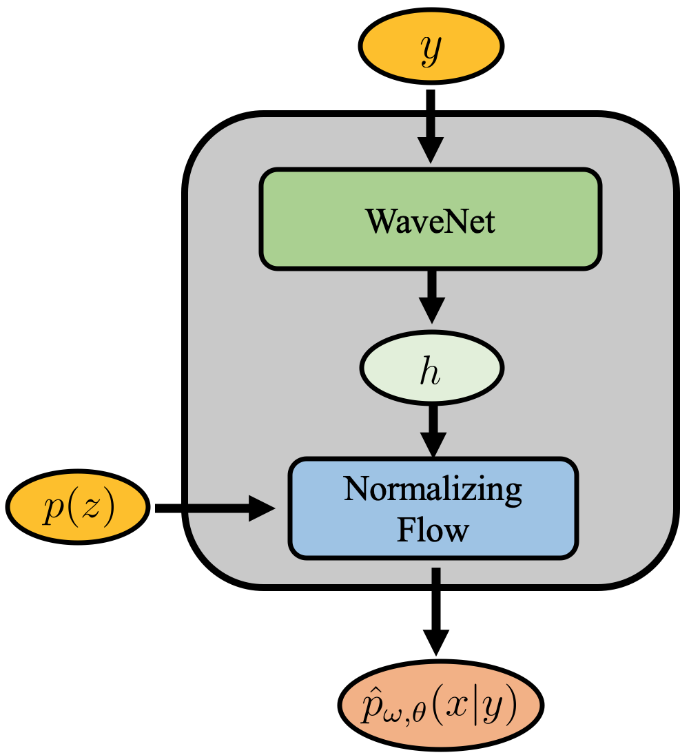
The computation of the transformation contains two steps. The first step is to compute the intermediate coefficients from the feature vector based on the function , which is parameterized by 2 fully connected layers with weights denoted as , i.e., . The coefficients are used to combine the invertible linear rational splines to form (see Eq. (5) in [64] for details). Therefore, is an element-wise invertible linear rational spline with coefficients . Since depends on the input waveform and , the resulting mapping and parameterized distribution in Eq. (2) vary with the input . The parameterization of the estimated posterior distribution is illustrated in Figure 1.
To learn the network weights, we need to construct the empirical loss objective given the collection of training data . We propose to include a loss term defined on the feature vectors in our learning objective to take account for the variation in the waveform due to noise. That is if the underlying physical parameters are similar, then the similarity of the feature vectors should be large, and vice versa. To achieve this, we use contrastive learning objective [68] to distinguish positive data pairs (waveforms with the same physical parameters) from the negative pairs (noisy waveforms with different physical parameters). Specifically, we use the normalized temperature-scaled cross entropy (NT-Xent) loss used in the state-of-the-art contrastive learning technique SimCLR [69, 70]. SimCLR was originally introduced to improve the performance of image classification with additional data augmentation and NT-Xent loss evaluation. We adapt the NT-Xent loss used in contrastive learning to our feature vectors,
| (3) |
where , is a scalar temperature parameter, and we choose according to the default setting provided in [69]. The NT-Xent loss performs in such a way that, regardless of the noise statistics, the cosine distances of the encoded features associated with the same underlying physical parameters (i.e. and ) are minimized, and the distances of features with different underlying physical parameters are maximized. Consequently, the trained model is robust to the change of noise realizations and noise statistics. Therefore, incorporating the term in Eq. (3) can be used as a noise stabilizer for gravitational wave parameter estimation. We found that the inclusion of this term speeds up the convergence in training.
Our deep learning objective in Eq. (2.1) combines the NT-Xent loss in Eq. (3) with the posterior approximation term. Given a batch of physical parameters , we generate different noise realizations for each and the empirical loss function is,
| (4) |
where is defined in Eq. (2). Minimizing the loss in Eq. (2.1) with respect to and provides a posterior estimation for gravitational wave events.
It is worth pointing out that while Refs. [71, 72] apply , an arbitrary random distribution to their generative model, our posterior distributions do not involve arbitrary random distributions.
2.2 Separate Models for Parameters
In this paper, we are interested in the following physical parameters: . We find that trying to estimate all parameters using a single model lead to sub-optimal results given that they are of different scales. Thus, we use two separate models with similar model architecture as shown in Figure 1. One model is used to estimate the masses of the binary components, while the other one is used to infer the final spin and QNMs of the remnant.
The final spin of the remnant and its QNMs have similar range of values when the QNMs are cast in dimensionless units. We trained the second model using the fact that the QNMs are determined by the final spin using the relation [56]:
| (5) |
where correspond to the frequency and damping time of the ringdown oscillations for the fundamental bar mode, and the first overtone . We compute the QNMs following [56]. One can translate into the ringdown frequency (in units of Hertz) and into the corresponding (inverse) damping time (in units of seconds) by computing , where is the final mass of the remnant, and can be determined using Eq. (1) in [73]. An additional benefit of using two separate models is that the training converges faster with two models considering two different sets of physical parameters at different magnitudes.
2.3 Dataset Preparation and Training
Modeled Waveforms We used the surrogate waveform family [74] to produce modeled waveforms that describe binary black holes with component masses , , and spin components . By uniformly sampling this parameter space we produce a dataset with 1,061,023 waveforms. These waveforms describe the last second of the late inspiral, merger, and ringdown. The waveforms are produced using a sample rate of 4096Hz.
For training purposes, we label the waveforms using the masses and spins of the binary components, and then use this information to also enable the neural net to estimate the final spin of the black hole remnant using the formulae provided in [75], and the QNMs following [56]. In essence, we are training our neural network models to identify the key features that determine the properties of the binary black holes before and after merger using a unified framework.
We use 90% of these waveform samples for training, 10% testing. The training samples are randomly and uniformly chosen. Throughout the training, we use AdamW optimizer to minimize the mean squared error of the predicted parameters with default hyper-parameter setups [76]. We choose the learning rate to be 0.0001. To simulate the environment where the true gravitational waves are embedded, we use real advanced LIGO noise to compute power spectral density (PSD), which is then used to whiten the templates.
Advanced LIGO noise. For training we used a 4096s-long advanced LIGO noise data segment, sampled at 4096Hz, starting at GPS time 1126259462. We obtained these data from the Gravitational Wave Open Science Center [41]. We estimate a PSD using the entire 4096s segment to whiten the modeled waveforms and noise. For each one second long noisy waveform used in training, we combine the clean whitened template with a randomly picked one second long noise segment from the 4096s-long advanced LIGO strain data. For each generated waveform template (see Eq. 1), we apply two different noisy realizations. As a result, the total number of noisy waveforms (clean templates noise realizations) applied during training is equal to: of training iterations batch size 2.
In Section 4, we demonstrate that our model, trained only with advanced LIGO noise from the first observing run, is able to estimate the astrophysical parameters of other events across O1-O3. We fixed the merger point of the training templates at the 3,596 timestep out of 4,096 total timesteps. We empirically found having a fixed merger point, rather than shifting the templates to have time-invariant property, provides a tighter estimation of the posteriors. Our deep learning model was trained on 1 NVIDIA V100 GPU with a batch size of 8. In general, it takes about 1-2 days to fully train this model.
2.4 GPS Trigger Time
It is known that a trigger GPS time associated with a gravitational wave event, typically provided by a detection algorithm, may differ from the true time of coalescence. Therefore, we perform a local search around the trigger time by any given detection algorithm as a pre-processing step for the parameter estimation using the trained model. We first identify local merger time candidates by evaluating the normalized cross-correlation (NCC) of the whitened observation with 33,713 whitened clean templates, whose physical parameters uniformly cover the range: , , and , over a time window of 0.015 seconds around the time candidates. The time points with top NCC values are selected as the candidates. Then we use the trained models to estimate the posterior distributions of the physical parameters at each candidate time point. In practice, we found that the trigger times with the best NCC values differ from those published at the Gravitational Wave Open Science Center by up to 0.01s. These trigger times produce different posterior distributions that vary in size by up to for the masses of the binary components, and up to 5% for the astrophysical properties of the compact remnant. We have selected the time point that gives the smallest confidence area for the results we present in Section 4.2.
3 Bayesian Inference
We compare our data-driven posterior estimation with PyCBC Inference [46, 59, 60], which uses a parallel-tempered MCMC algorithm, emcee_pt [77], to evaluate the posterior probability for the set of source parameters given the data . The posterior is calculated as where is the likelihood and is the prior. The likelihood function for a set of detectors is
| (6) |
where and are the frequency-domain representations of the data and the model waveform for detector . The inner product is defined as
| (7) |
where is the PSD of the -th detector.
We performed the MCMC analysis using the publicly available data from the GWTC-1 release [4] and used the corresponding publicly available PSD files for each event [78]. We analyse a segment of 8 seconds around the GPS trigger 1167559935.6, with the data sampled to 2048 Hz. We use the IMRPhenomD [79] waveform model to generate waveform templates to evaluate the likelihood. We assume uniform priors for the component masses with and uniform priors on the component spins with . We also set uniform priors on the luminosity distance with and the deviation of the arrival time from the trigger time . We set uniform priors for the coalescence phase and the polarization angle . The prior on the inclination angle between the binary’s orbital angular momentum and the line of sight, , is set to be uniform in the sine of the angle, and the right ascension and declination have priors to be uniform over the sky.
Furthermore, they may be used to cross validate the physical reality of an event [39, 40], and to assess whether the estimated merger time is consistent between the two separate models. For instance, if the models output very different merger times, then we may conclude that they are not providing a reliable merger time. On the other hand, when their results are consistent, within a window between 0.001s and up to 0.005s, then we can remove the ambiguity introduced when using the NCC approach described in Section 2.4.
4 Experimental Results
In this section we present two types of results. First, we validate our model with a well known statistical model. Upon confirming that our deep learning approach is statistically consistent, we used to estimate the parameters of five binary black hole mergers.
4.1 Validation on Simulated Data
We performed experiments on simulated data that have closed form posterior distributions. This is important to ascertain the accuracy and reliability of our method. The simulated data are generated through a linear observation model with additive white Gaussian noise,
| (8) |
where the additive noise . We consider the underlying parameters and the linear map , with and . The likelihood function is
| (9) |
If we assume the prior distribution of is a Gaussian distribution with mean and covariance , we can get an analytical expression for the posterior distribution of given the observation ,
| (10) |
where
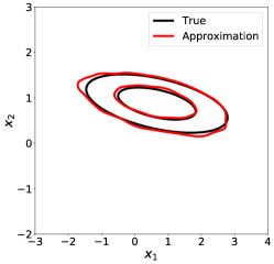
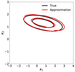
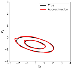
During the training stage we draw 100 samples of from its prior , and is generated through the linear observation model (8). We train a 3-layer model with the model objective (2.1), and show three examples of the posterior estimation in Figure 2. Therein we show 50% and 90% confidence contours. Black lines represent ground truth results (ellipses given the posterior is Gaussian), while the red contours correspond to the neural network estimations, based on Gaussian kernel density estimation (KDE) with 9,000 samples generated from the network. These results indicate that our deep learning model can produce reliable and statistically valid results.
| Event Name | Our model | LIGO [4, 80] | SNR | ||
|---|---|---|---|---|---|
| GW150914 | 24.4 | ||||
| GW170104 | 13.0 | ||||
| GW170814 | 15.9 | ||||
| GW190521 | 14.4 | ||||
| GW190630 | 15.6 | ||||
| Event Name | Our model | LIGO [4, 80] | ||||
|---|---|---|---|---|---|---|
| GW150914 | ||||||
| GW170104 | ||||||
| GW170814 | ||||||
| GW190521 | ||||||
| GW190630 | ||||||
4.2 Results with Real Events
In this section we use our deep learning models to estimate the medians and posterior distributions of the astrophysical parameters and , respectively, for five binary black hole mergers: GW150914, GW170104, GW170814, GW190521 and GW190630.
As described in Section 2.1, we consider 1s-long advanced LIGO noise input data batches, denoted as , sampled at 4096Hz. We construct two posterior distribution estimations, , by minimizing the loss in Eq. (2.1) for and for . We use two different multivariate normal base distributions for in the two different models. To estimate the masses of the binary components, the mean and covariance matrix () are: ; whereas for the final spin and QNMs model we use: . “” refers to the diagonal matrix with “” being the diagonal elements. The number of normalizing flow layers also varies for the two models. We use a 3-layer normalizing flow module for masses prediction, and an 8-layer module for the predictions of final spin and QNMs.
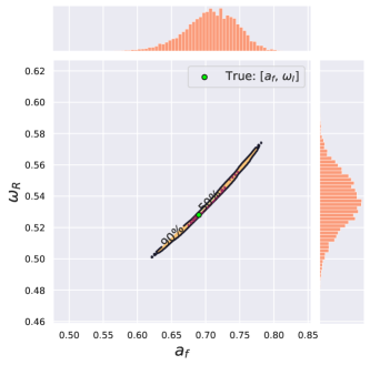
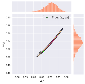
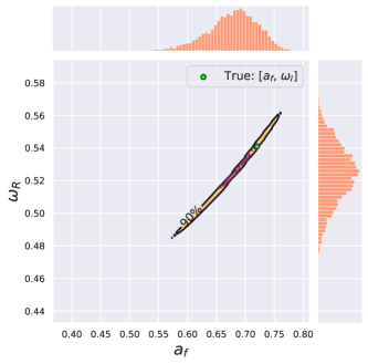
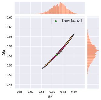
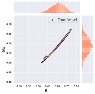
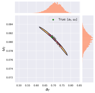
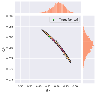
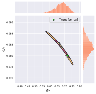
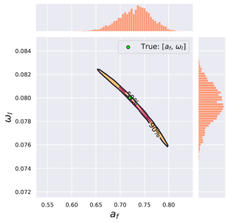
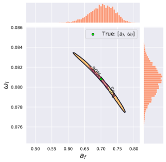
Our first set of results is presented in Figures 3, 4, and 5. These figures provide the median, and the 50% and 90% confidence intervals, which we computed using Gaussian KDE estimation with 9,000 samples drawn from the estimated posteriors. In Tables 1 and 2 we also present a summary of our data-driven median results and 90% confidence intervals, along with those obtained with traditional Bayesian algorithms in [4, 80].
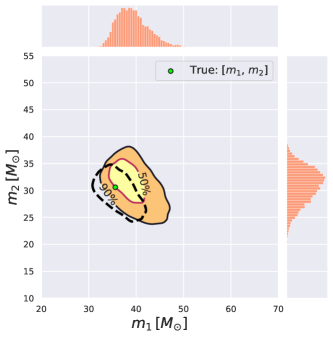
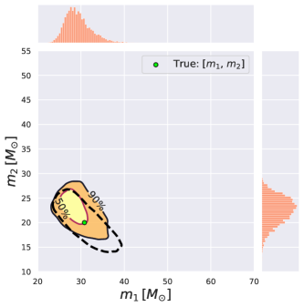
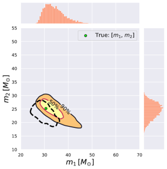
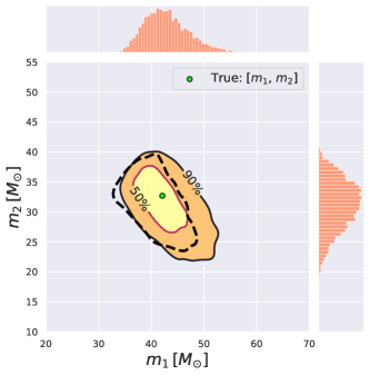
Before we present the main highlights of these results, it is important to emphasize that our results are entirely data-driven. We have not attempted to use deep learning as a fast interpolator that learns the properties of traditional Bayesian posterior distributions. Rather, we have allowed deep learning to figure out the physical correlations among different parameters that describe the physics of black hole mergers. Furthermore, we have quantified the statistical consistency of our approach by validating it against a well known model. This is of paramount importance, since deep learning models may be constructed to reproduce the properties of traditional Bayesian distributions, but that fact does not provide enough evidence of their statistical validity or consistency. Finally, given the nature of the signal processing tools and computing approaches we use in this study, we do not expect our data-driven results to exactly reproduce the traditional Bayesian results reported in [4, 80].
Our results may be summarized as follows. Figures 3, 4, and 5 show that our data-driven posterior distributions encode expected physical correlations for the masses of the binary components, , and the parameters of the remnant: and . We also learn that these posterior distributions are determined by the properties of the noise and loudness of the signal that describes these events. Figure 3 presents a direct comparison between the posterior distributions predicted by our deep learning models and those produced with PyCBC Inference—marked with dashed lines. These results show that our deep learning models provide real-time, reliable information about the astrophysical properties of binary black hole mergers that were detected in three different observing runs, and which span a broad SNR range.
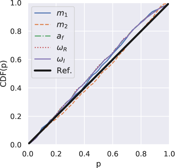
On the other hand, Tables 1 and 2 show that our median and 90% confidence intervals are better, similar and in some cases slightly larger than those obtained with Bayesian algorithms. In these Tables, Bayesian LIGO results for are directly taken from [4, 80], while results are computed using their Bayesian results for and the tables available at [82]. These results indicate that deep learning methods can learn physical correlations in the data, and provide reliable estimates of the parameters of gravitational wave sources. To demonstrate that our model represents true statistical properties of the posterior distribution, we tested the posterior estimation on simulated noisy gravitational waveforms. We calculate the empirical cumulative distribution function (CDF) of the number of times the true value for each parameter was found within a given confidence interval , as a function of . We compare the empirical CDF with the true CDF of in the P-P plot in Figure 6. To obtain the empirical CDF, for each test waveform (1000 waveforms in total) and one-dimensional estimated posterior distribution generated from the network with 9,000 samples, we record the count of the confidence intervals (=1% , …, 100%) where the true parameters fall. The empirical CDF is based on the frequency of such counts with the 1000 waveforms randomly drawn from the test dataset. Since the empirical CDFs lie close to the diagonal, we conclude that the networks generate close approximation of the posteriors. Furthermore, our data-driven results, including medians and posterior distributions, can be produced within 2 milliseconds per event using a single NVIDIA V100 GPU. We expect that these tools will provide the means to assess in real-time whether the inferred astrophysical parameters of the binary components and the post-merger remnant adhere to general relativistic predictions. If not, these results may prompt follow up analyses to investigate whether apparent discrepancies are due to poor data quality or other astrophysical effects [83].
The reliable astrophysical information inferred in low-latency by deep learning algorithm warrants the extension of this framework to characterize other sources, including eccentric compact binary mergers, and sources that require the inclusion of higher-order waveform modes. Furthermore, the use of physics-inspired deep learning architectures and optimization schemes [29] may enable an accurate measurement of the spin of binary components. These studies should be pursued in the future.
5 Conclusion
We designed neural networks to estimate five parameters that describe the astrophysical properties of binary black holes before and after the merger event. The first two parameters constrain the masses of the binary components, while the others estimate the properties of the black hole remnant, namely . These models combine a WaveNet architecture with normalizing flow and contrastive learning to provide statistically consistent estimates for both simulated distributions, and real gravitational wave sources.
Our findings indicate that deep learning can abstract physical correlations in complex data, and then provide reliable predictions for the median and 90% confidence intervals for binary black holes that span a broad SNR range. Furthermore, while these models were trained using only advanced LIGO noise from the first observing run, they were capable of generalizing to binary black holes that were reported during the first, second and third observing runs.
These models will be extended in future work to provide informative estimates for the spin of the binary components, including higher-order waveform modes to better model the physics of highly spinning and asymmetric mass-ratio black hole systems.
6 Acknowledgements
Neural network models are available at the Data and Deep Learning Hub for Science [84, 85]. EAH, HS and ZZ gratefully acknowledge National Science Foundation (NSF) awards OAC-1931561 and OAC-1934757. EOS and PK gratefully acknowledge NSF grants PHY-1912081 and OAC-193128, and the Sherman Fairchild Foundation. PK also acknowledges the support of the Department of Atomic Energy, Government of India, under project no. RTI4001. This work utilized the Hardware-Accelerated Learning (HAL) cluster, supported by NSF Major Research Instrumentation program, grant OAC-1725729, as well as the University of Illinois at Urbana-Champaign. Compute resources were provided by XSEDE using allocation TG-PHY160053. This work made use of the Illinois Campus Cluster, a computing resource that is operated by the Illinois Campus Cluster Program (ICCP) in conjunction with the National Center for Supercomputing Applications and which is supported by funds from the University of Illinois at Urbana-Champaign. This research used resources of the Argonne Leadership Computing Facility, which is a DOE Office of Science User Facility supported under Contract DE-AC02-06CH11357. This research also made use of LIGO Data Grid clusters at the California Institute of Technology. This research used data, software and/or web tools obtained from the LIGO Open Science Center (https://gw-openscience.org), a service of LIGO Laboratory, the LIGO Scientific Collaboration and the Virgo Collaboration. LIGO is funded by the U.S. National Science Foundation. Virgo is funded by the French Centre National de Recherche Scientifique (CNRS), the Italian Istituto Nazionale della Fisica Nucleare (INFN) and the Dutch Nikhef, with contributions by Polish and Hungarian institutes.
References
- [1] Abbott B P, Abbott R, Abbott T D, Abernathy M R, Acernese F, Ackley K, Adams C, Adams T, Addesso P, Adhikari R X and et al 2016 Physical Review Letters 116 131103 (Preprint 1602.03838)
- [2] Aasi J, Abbott B, Abbott R, Abbott T, Abernathy M, Ackley K, Adams C, Adams T, Addesso P, Adhikari R et al. 2015 Classical and quantum gravity 32 074001
- [3] Acernese F et al. 2015 Classical and Quantum Gravity 32 024001 (Preprint 1408.3978)
- [4] Abbott B P et al. (LIGO Scientific Collaboration and Virgo Collaboration) 2019 Phys. Rev. X 9(3) 031040 URL https://link.aps.org/doi/10.1103/PhysRevX.9.031040
- [5] Abbott R et al. (LIGO Scientific, Virgo) 2021 Phys. Rev. X 11 021053 (Preprint 2010.14527)
- [6] Abbott R et al. (LIGO Scientific, Virgo) 2021 Astrophys. J. Lett. 913 L7 (Preprint 2010.14533)
- [7] Huerta E, Haas R, Fajardo E, Katz D S, Anderson S, Couvares P, Willis J, Bouvet T, Enos J, Kramer W T et al. 2017 Boss-ldg: a novel computational framework that brings together blue waters, open science grid, shifter and the ligo data grid to accelerate gravitational wave discovery 2017 IEEE 13th International Conference on e-Science (e-Science) (IEEE) pp 335–344
- [8] Huerta E, Haas R, Jha S, Neubauer M and Katz D S 2019 Computing and Software for Big Science 3 5
- [9] Weitzel D, Bockelman B, Brown D A, Couvares P, Würthwein F and Hernandez E F 2017 Data access for ligo on the osg Proceedings of the Practice and Experience in Advanced Research Computing 2017 on Sustainability, Success and Impact pp 1–6
- [10] Liang S, Liu Y, Wang C and Jian L 2010 Design and evaluation of a parallel k-nearest neighbor algorithm on CUDA-enabled GPU 2010 IEEE 2nd Symposium on Web Society pp 53–60 ISSN 2158-6985
- [11] Allen G, Anderson W, Blaufuss E, Bloom J S, Brady P, Burke-Spolaor S, Cenko S B, Connolly A, Couvares P, Fox D, Gal-Yam A, Gezari S, Goodman A, Grant D, Groot P, Guillochon J, Hanna C, Hogg D W, Holley-Bockelmann K, Howell D A, Kaplan D, Katsavounidis E, Kowalski M, Lehner L, Muthukrishna D, Narayan G, Peek J E G, Saha A, Shawhan P and Taboada I 2018 arXiv e-prints arXiv:1807.04780 (Preprint 1807.04780)
- [12] Allen G, Andreoni I, Bachelet E, Berriman G B, Bianco F B, Biswas R, Carrasco Kind M, Chard K, Cho M, Cowperthwaite P S, Etienne Z B, George D, Gibbs T, Graham M, Gropp W, Gupta A, Haas R, Huerta E A, Jennings E, Katz D S, Khan A, Kindratenko V, Kramer W T C, Liu X, Mahabal A, McHenry K, Miller J M, Neubauer M S, Oberlin S, Olivas Alexander R J, Rosofsky S, Ruiz M, Saxton A, Schutz B, Schwing A, Seidel E, Shapiro S L, Shen H, Shen Y, Sipőcz B M, Sun L, Towns J, Tsokaros A, Wei W, Wells J, Williams T J, Xiong J and Zhao Z 2019 arXiv e-prints arXiv:1902.00522 (Preprint 1902.00522)
- [13] Huerta E A, Allen G, Andreoni I, Antelis J M, Bachelet E, Berriman G B, Bianco F B, Biswas R, Carrasco Kind M, Chard K, Cho M, Cowperthwaite P S, Etienne Z B, Fishbach M, Forster F, George D, Gibbs T, Graham M, Gropp W, Gruendl R, Gupta A, Haas R, Habib S, Jennings E, Johnson M W G, Katsavounidis E, Katz D S, Khan A, Kindratenko V, Kramer W T C, Liu X, Mahabal A, Marka Z, McHenry K, Miller J M, Moreno C, Neubauer M S, Oberlin S, Olivas A R, Petravick D, Rebei A, Rosofsky S, Ruiz M, Saxton A, Schutz B F, Schwing A, Seidel E, Shapiro S L, Shen H, Shen Y, Singer L P, Sipocz B M, Sun L, Towns J, Tsokaros A, Wei W, Wells J, Williams T J, Xiong J and Zhao Z 2019 Nature Reviews Physics 1 600–608 (Preprint 1911.11779)
- [14] George D and Huerta E A 2018 Phys. Rev. D 97(4) 044039 (Preprint 1701.00008) URL https://link.aps.org/doi/10.1103/PhysRevD.97.044039
- [15] George D and Huerta E A 2017 Deep Learning for Real-time Gravitational Wave Detection and Parameter Estimation with LIGO Data NiPS Summer School 2017 Gubbio, Perugia, Italy, June 30-July 3, 2017 (Preprint 1711.07966)
- [16] George D and Huerta E 2018 Physics Letters B 778 64 – 70 ISSN 0370-2693 URL http://www.sciencedirect.com/science/article/pii/S0370269317310390
- [17] Gabbard H, Williams M, Hayes F and Messenger C 2018 Physical Review Letters 120 141103 (Preprint 1712.06041)
- [18] Skliris V, Norman M R and Sutton P J 2020 arXiv preprint arXiv:2009.14611
- [19] Lin Y C and Wu J H P 2020 arXiv preprint arXiv:2007.04176
- [20] Wang H, Wu S, Cao Z, Liu X and Zhu J Y 2020 Phys. Rev. D 101 104003 (Preprint 1909.13442)
- [21] Nakano H, Narikawa T, Oohara K i, Sakai K, Shinkai H a, Takahashi H, Tanaka T, Uchikata N, Yamamoto S and Yamamoto T S 2019 Phys. Rev. D 99 124032 (Preprint 1811.06443)
- [22] Fan X, Li J, Li X, Zhong Y and Cao J 2019 Sci. China Phys. Mech. Astron. 62 969512 (Preprint 1811.01380)
- [23] Li X R, Babu G, Yu W L and Fan X L 2020 Front. Phys. (Beijing) 15 54501 (Preprint 1712.00356)
- [24] Deighan D S, Field S E, Capano C D and Khanna G 2020 (Preprint 2010.04340)
- [25] Miller A L et al. 2019 Phys. Rev. D 100 062005 (Preprint 1909.02262)
- [26] Krastev P G 2020 Phys. Lett. B 803 135330 (Preprint %****␣iop_gwparam_revision.bbl␣Line␣150␣****1908.03151)
- [27] Schäfer M B, Ohme F and Nitz A H 2020 Phys. Rev. D 102 063015 (Preprint 2006.01509)
- [28] Dreissigacker C and Prix R 2020 Phys. Rev. D 102 022005 (Preprint 2005.04140)
- [29] Khan A, Huerta E and Das A 2020 Phys. Lett. B 808 0370–2693 (Preprint 2004.09524)
- [30] Dreissigacker C, Sharma R, Messenger C, Zhao R and Prix R 2019 Phys. Rev. D 100 044009 (Preprint 1904.13291)
- [31] Wei W, Huerta E A, Whitmore B C, Lee J C, Hannon S, Chandar R, Dale D A, Larson K L, Thilker D A, Ubeda L, Boquien M, Chevance M, Kruijssen J M D, Schruba A, Blanc G A and Congiu E 2020 MNRAS 493 3178–3193 (Preprint 1909.02024)
- [32] Beheshtipour B and Papa M A 2020 Phys. Rev. D 101 064009 (Preprint 2001.03116)
- [33] Skliris V, Norman M R K and Sutton P J 2020 arXiv e-prints arXiv:2009.14611 (Preprint 2009.14611)
- [34] Khan S and Green R 2020 arXiv preprint arXiv:2008.12932
- [35] Chua A J K, Galley C R and Vallisneri M 2019 Phys. Rev. Lett. 122(21) 211101 URL https://link.aps.org/doi/10.1103/PhysRevLett.122.211101
- [36] Rebei A, Huerta E A, Wang S, Habib S, Haas R, Johnson D and George D 2019 Phys. Rev. D100 044025 (Preprint 1807.09787)
- [37] Wei W and Huerta E A 2021 Physics Letters B 816 136185 (Preprint 2010.09751)
- [38] Wei W, Huerta E A, Yun M, Loutrel N, Shaikh M A, Kumar P, Haas R and Kindratenko V 2021 Astrophys. J. 919 82 (Preprint 2012.03963)
- [39] Huerta E A, Khan A, Huang X, Tian M, Levental M, Chard R, Wei W, Heflin M, Katz D S, Kindratenko V, Mu D, Blaiszik B and Foster I 2021 Nature Astronomy 5 1062–1068 (Preprint 2012.08545)
- [40] Wei W, Khan A, Huerta E A, Huang X and Tian M 2021 Physics Letters B 812 136029 (Preprint 2010.15845)
- [41] Vallisneri M, Kanner J, Williams R, Weinstein A and Stephens B 2015 J. Phys. Conf. Ser. 610 012021 (Preprint 1410.4839)
- [42] Yu H, Adhikari R X, Magee R, Sachdev S and Chen Y 2021 arXiv e-prints arXiv:2104.09438 (Preprint 2104.09438)
- [43] Graff P, Feroz F, Hobson M P and Lasenby A 2012 MNRAS 421 169–180 (Preprint 1110.2997)
- [44] Veitch J, Raymond V, Farr B, Farr W, Graff P, Vitale S, Aylott B, Blackburn K, Christensen N, Coughlin M, Del Pozzo W, Feroz F, Gair J, Haster C J, Kalogera V, Littenberg T, Mandel I, O’Shaughnessy R, Pitkin M, Rodriguez C, Röver C, Sidery T, Smith R, Van Der Sluys M, Vecchio A, Vousden W and Wade L 2015 Phys. Rev. D 91 042003 (Preprint 1409.7215)
- [45] Singer L P and Price L R 2016 Physical Review D 93 024013 (Preprint 1508.03634)
- [46] Biwer C M, Capano C D, De S, Cabero M, Brown D A, Nitz A H and Raymond V 2019 The Astronomical Society of the Pacific 131 024503 (Preprint 1807.10312)
- [47] Alvares J D, Font J A, Freitas F F, Freitas O G, Morais A P, da Silva Nunes S, Onofre A and Torres-Forné A 2021 Classical and Quantum Gravity
- [48] Chua A J K and Vallisneri M 2020 Phys. Rev. Lett. 124 041102 (Preprint 1909.05966)
- [49] Gabbard H, Messenger C, Heng I S, Tonolini F and Murray-Smith R 2019 arXiv preprint arXiv:1909.06296 (Preprint 1909.06296)
- [50] Green S R, Simpson C and Gair J 2020 Phys. Rev. D 102 104057 (Preprint 2002.07656)
- [51] Green S R and Gair J 2021 Mach. Learn. Sci. Tech. 2 03LT01 (Preprint 2008.03312)
- [52] Grover A, Dhar M and Ermon S 2018 Flow-gan: Combining maximum likelihood and adversarial learning in generative models AAAI
- [53] Dax M, Green S R, Gair J, Macke J H, Buonanno A and Schölkopf B 2021 arXiv e-prints arXiv:2106.12594 (Preprint 2106.12594)
- [54] Cuoco E, Powell J, Cavaglià M, Ackley K, Bejger M, Chatterjee C, Coughlin M, Coughlin S, Easter P, Essick R et al. 2020 Machine Learning: Science and Technology 2 011002
- [55] Huerta E A and Zhao Z 2020 Advances in Machine and Deep Learning for Modeling and Real-Time Detection of Multi-messenger Sources (Singapore: Springer Singapore) pp 1–27 ISBN 978-981-15-4702-7 URL https://doi.org/10.1007/978-981-15-4702-7_47-1
- [56] Berti E, Cardoso V and Will C M 2006 Phys. Rev. D 73 064030–+ (Preprint arXiv:gr-qc/0512160)
- [57] Övgün A, Sakallı İ and Mutuk H 2021 International Journal of Geometric Methods in Modern Physics 2150154
- [58] Paszke A, Gross S, Chintala S, Chanan G, Yang E, DeVito Z, Lin Z, Desmaison A, Antiga L and Lerer A 2017 Automatic differentiation in pytorch NIPS-W
- [59] Nitz A, Harry I, Brown D et al. 2020 gwastro/pycbc: Pycbc release 1.16.4 URL https://doi.org/10.5281/zenodo.3904502
- [60] Vousden W D, Farr W M and Mandel I 2015 Monthly Notices of the Royal Astronomical Society 455 1919–1937 ISSN 1365-2966 URL http://dx.doi.org/10.1093/mnras/stv2422
- [61] van den Oord A, Dieleman S, Zen H, Simonyan K, Vinyals O, Graves A, Kalchbrenner N, Senior A and Kavukcuoglu K 2016 arXiv preprint arXiv:1609.03499
- [62] Wei W and Huerta E 2020 Physics Letters B 800 135081
- [63] Durkan C, Bekasov A, Murray I and Papamakarios G 2019 Neural spline flows Advances in Neural Information Processing Systems pp 7511–7522
- [64] Dolatabadi H M, Erfani S and Leckie C 2020 arXiv preprint arXiv:2001.05168
- [65] Bingham E, Chen J P, Jankowiak M, Obermeyer F, Pradhan N, Karaletsos T, Singh R, Szerlip P, Horsfall P and Goodman N D 2019 The Journal of Machine Learning Research 20 973–978
- [66] Bingham E, Chen J P, Jankowiak M, Obermeyer F, Pradhan N, Karaletsos T, Singh R, Szerlip P, Horsfall P and Goodman N D 2018 Journal of Machine Learning Research
- [67] Phan D, Pradhan N and Jankowiak M 2019 arXiv preprint arXiv:1912.11554
- [68] Hadsell R, Chopra S and LeCun Y 2006 Dimensionality reduction by learning an invariant mapping 2006 IEEE Computer Society Conference on Computer Vision and Pattern Recognition (CVPR’06) vol 2 (IEEE) pp 1735–1742
- [69] Chen T, Kornblith S, Norouzi M and Hinton G 2020 A simple framework for contrastive learning of visual representations Thirty-seventh International Conference on Machine Learning
- [70] Chen T, Kornblith S, Swersky K, Norouzi M and Hinton G E 2020 Advances in Neural Information Processing Systems 33
- [71] Dumoulin V, Belghazi I, Poole B, Lamb A, Arjovsky M, Mastropietro O and Courville A C 2017 ArXiv abs/1606.00704
- [72] Donahue J, Krähenbühl P and Darrell T 2017 ArXiv abs/1605.09782
- [73] Healy J and Lousto C O 2017 Phys. Rev. D 95 024037
- [74] Blackman J, Field S E, Galley C R, Szilágyi B, Scheel M A, Tiglio M and Hemberger D A 2015 Physical Review Letters 115 121102 (Preprint 1502.07758)
- [75] Hofmann F, Barausse E and Rezzolla L 2016 Astrophys. J. 825 L19
- [76] Loshchilov I and Hutter F 2017 arXiv preprint arXiv:1711.05101
- [77] Foreman-Mackey D, Hogg D W, Lang D and Goodman J 2013 The Astronomical Society of the Pacific 125 306 (Preprint 1202.3665)
- [78] 2019 Parameter estimation sample release for GWTC-1 URL https://dcc.ligo.org/LIGO-P1800370/public
- [79] Khan S, Husa S, Hannam M, Ohme F, Pürrer M, Forteza X J and Bohé A 2016 Phys. Rev. D 93(4) 044007 URL https://link.aps.org/doi/10.1103/PhysRevD.93.044007
- [80] Abbott R, Abbott T, Abraham S, Acernese F, Ackley K, Adams A, Adams C, Adhikari R, Adya V, Affeldt C et al. 2020 arXiv preprint arXiv:2010.14527
- [81] Berti E, Cardoso V and Casals M 2006 Phys. Rev. D 73 024013 (Preprint arXiv:gr-qc/0511111)
- [82] Berti E, Buonanno A and Will C M 2005 Phys. Rev. D 71 084025 (Preprint gr-qc/0411129)
- [83] Gair J R, Vallisneri M, Larson S L and Baker J G 2013 Living Rev. Rel. 16 7 (Preprint 1212.5575)
- [84] Blaiszik B, Ward L, Schwarting M, Gaff J, Chard R, Pike D, Chard K and Foster I 2019 MRS Communications 9
- [85] Chard R, Li Z, Chard K, Ward L, Babuji Y, Woodard A, Tuecke S, Blaiszik B, Franklin M J and Foster I 2019 Dlhub: Model and data serving for science 2019 IEEE International Parallel and Distributed Processing Symposium (IPDPS) pp 283–292