Real-time gravitational-wave science with neural posterior estimation
Abstract
We demonstrate unprecedented accuracy for rapid gravitational-wave parameter estimation with deep learning. Using neural networks as surrogates for Bayesian posterior distributions, we analyze eight gravitational-wave events from the first LIGO-Virgo Gravitational-Wave Transient Catalog and find very close quantitative agreement with standard inference codes, but with inference times reduced from to 20 seconds per event. Our networks are trained using simulated data, including an estimate of the detector-noise characteristics near the event. This encodes the signal and noise models within millions of neural-network parameters, and enables inference for any observed data consistent with the training distribution, accounting for noise nonstationarity from event to event. Our algorithm—called “DINGO”—sets a new standard in fast-and-accurate inference of physical parameters of detected gravitational-wave events, which should enable real-time data analysis without sacrificing accuracy.
Introduction.—Since the first detection of a signal from a pair of merging black holes [1], gravitational waves have quickly emerged as an important new probe of gravitational theory [2], neutron-star physics [3], cosmology [4], and black-hole astrophysics [5]. These scientific successes were made possible by a growing rate of detections by the LIGO [6] and Virgo [7] observatories, and their subsequent analysis and characterization as signals from merging compact binary systems. The LIGO and Virgo Collaborations (LVC) have now published results from over 50 such systems [8, 9], and this number promises to grow ever-faster as detectors are made more sensitive in the future [10].
Given a detection, Bayesian inference is used to characterize the originating source [11]. This is based on having models for the signals and the detector noise. For gravitational waves, signal models take the form of waveform predictions depending on the source parameters (masses, location, etc.). Waveform models are based on solutions to Einstein’s equations (and any relevant matter equations) for the two-body dynamics and gravitational radiation, using a combination of numerical-relativity and perturbative calculations [12, 13, 14] and phenomenological fitting [15, 16, 14]. Detector noise is typically modeled as stationary and Gaussian, with some spectrum which can be estimated empirically. Together, these “forward” models give rise to the likelihood for the observed strain data , which is assumed to consist of a signal plus noise. With the choice of a prior over parameters, the posterior distribution is given via Bayes’ theorem,
| (1) |
where is a normalizing factor called the evidence. The posterior gives our belief about the source parameters, given the observed data.
The task of inference is to characterize the posterior by drawing samples from it. This can be accomplished with stochastic algorithms like Markov chain Monte Carlo (MCMC). The LVC have developed software tools such as LALInference [17] and Bilby [18, 19, 20] to carry this out. However, these algorithms are computationally expensive as they require many likelihood evaluations for each independent posterior sample , and each likelihood requires a waveform simulation. An analysis producing independent samples typically requires millions of waveform evaluations and a total inference time of hours to months, depending on the signal duration and waveform model. More physically-realistic waveform models [21] are also more costly, so carrying out inference for all events with the best models is an enormous computational effort. When rapid results are desired—for alerts to trigger electromagnetic follow-up of transient phenomena [22], or when processing large numbers of events—accuracy usually has to be traded off for speed, by restricting to a limited set of fast models [23, 24] or specialized inference algorithms [25, 26, 27].
In this Letter, we describe an alternative approach to gravitational-wave inference which delivers both dramatically reduced analysis time and high accuracy, in stark contrast to the trade-off intrinsic to standard algorithms. The basic idea is to produce a large number of simulated data sets (with associated parameters), and use these to train a type of neural network known as a normalizing flow to approximate the posterior. The trained network can then generate new posterior samples extremely quickly once a detection is made. This bypasses the need to generate waveforms at inference time, thereby amortizing the expensive training costs over all future detections. The general approach of building such “surrogate” inverse models is called neural posterior estimation (NPE) [28, 29, 30], and is beginning to see application in several scientific domains [31]. When applied to gravitational waves, with all of the optimizations we describe, we call the method Deep INference for Gravitational-wave Observations, or DINGO.
NPE and conventional methods both involve the same inputs: a prior and a likelihood. A key difference, however, is the way in which the likelihood is used: for conventional methods, its density is evaluated, whereas for NPE it is used to simulate data, i.e., . This distinction is important when dealing with nonstationary or non-Gaussian detector noise, for which an analytic likelihood is either expensive or unavailable. In this case, one could nevertheless simulate data, in a noise-model-independent way, by injecting simulated signals into real noise. Our present focus is on speed and on validating DINGO on real data with the common assumption of stationary-Gaussian noise, but the ultimate aim of more accurate inference using real noise should be kept in mind.
There have been several previous studies that applied NPE or related approaches to gravitational waves [32, 33, 34, 35, 36, 37, 38, 39]; see also [40]. However, most of these are limited in some way: they either restrict the number of parameters or the distributional form of the posterior, or they do not analyze real data, or there are clear deviations from results obtained using standard algorithms. The best performance to-date was achieved in the study [36] by some of us. This was the only study to infer all 15 parameters111Parameters consist of detector-frame component masses , time of coalescence at geocenter , reference phase , sky position , luminosity distance , inclination angle , spin magnitudes , spin angles [41], and polarization angle . of a binary black hole (BBH) system in real data and demonstrate close agreement to standard samplers. However, even that study did not achieve full amortization, as it did not address the fact that detector noise varies from event to event. Rather, the neural network of [36] was tuned to the noise power spectral densities (PSDs) of the detectors at the time of the event analyzed, and it would require retraining for each new event.
We now present for the first time completely amortized inference for BBHs using DINGO. This is achieved by conditioning the neural network not only on the event strain data, but also on the detector noise PSD, which can be estimated using nearby data [17]. We also achieve unprecedented accuracy thanks to a new iterative algorithm for time-shifting the coalescence times, as well as various architecture improvements. We use our trained networks to analyze all events in the first Gravitational-Wave Transient Catalog (GWTC-1) [8] with component masses greater than (our prior bound) and find close (sometimes indistinguishable) quantitative agreement with standard algorithms. This Letter sets a new standard for rapid gravitational-wave inference, which should enable real-time gravitational-wave science in the near future. It shows that NPE has moved beyond toy models and is competitive with conventional algorithms. More broadly, it provides a demonstration of these new methods in a realistic use case, which we hope will inspire wider adoption in experimental science.
Method.—The central object of DINGO is the density-estimation neural network, which defines a conditional probability distribution . This should be distinguished from the posterior , which learns to approximate through training. We use so-called normalizing flows [42, 43, 44] to define a sufficiently flexible via a -dependent mapping from a simple “base” distribution ,
| (2) |
If can be rapidly evaluated and sampled from, and if is invertible and has simple Jacobian determinant, then can also be rapidly evaluated and sampled from. Following [36], we take to be multivariate standard normal, and a composition of spline coupling flows [45], each of which is defined with a neural network.
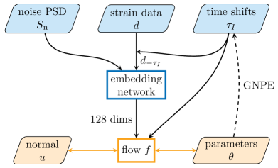
The overall structure of DINGO is illustrated in Fig. 1. This contains three key enhancements compared to the study [36]. First, since the data generation process depends on the detector noise PSD , we include this as additional context to the neural network, i.e., . This allows us to tune the network at inference time to the PSD estimated just prior to the event, corresponding to standard “off-source” noise estimation [17]. An alternative would be to estimate the noise “on-source” [46], but since we consider only short-duration BBH events here, the off-source approach is sufficient.
The second enhancement addresses the problem of high-dimensional observed data by using an additional neural network to first compress to a small number of features. This network (called an “embedding network”) is trained alongside the flow network. Our data is in the frequency domain, between 20 Hz and 1024 Hz, with 0.125 Hz resolution, so combined with the PSDs, this gives 24,096 input dimensions for each of the two or three interferometers. The first stage of the embedding network maps this linearly to 400 components per detector. To provide an inductive bias to extract signal information, we seed this layer with the principal components of clean waveforms from our training set, and then allow these parameters to float during training. Following this, a fully-connected residual network [47] compresses to 128 features, which are provided to the flow.
Finally, we developed a new method to treat time translations of the strain data. For standard algorithms, inference of requires sampling over waveforms with varying coalescence times in each detector . Likewise for NPE, the network must learn to interpret strain data with different . For frequency-domain data, however, time translations correspond to local phase shifts, which, although explicitly known, are challenging for neural networks to learn. Indeed, this occupied much of the network capacity in Ref. [36]. Our new approach—called group equivariant neural posterior estimation (GNPE)—leverages explicit knowledge of the time-translation symmetry along with approximate knowledge of to simplify the data representation and allow the network to focus on more nontrivial parameters. For further details see [48].
For GNPE, we train the network to infer given perturbed coalescence times and manually-time-shifted strain data . Using maximum likelihood estimation [49], this means we minimize the loss function
| (3) |
with respect to the network parameters [50]. Here, refers to the expected value over the specified distribution, which is evaluated stochastically using Monte Carlo draws. is a uniform kernel used to perturb . For inference, even though we do not have direct access to , all parameters can be inferred using Gibbs sampling starting with an approximate (obtained, e.g., using standard NPE): first, convolve with to obtain , then use the network to infer a new estimate for ; then convolve again and repeat. We find that this converges after iterations.
Evaluating (Real-time gravitational-wave science with neural posterior estimation) requires sampling and , and then simulating data . Aside from the PSD sampling, this follows Ref. [36] very closely. In particular we use the same prior over parameters, with . We train separate networks for the noise distributions in the first (O1) and second (O2) observing runs of LIGO and Virgo, with PSD samples estimated empirically from stretches of interferometer noise data [51]. For O1, we choose the distance prior Mpc. For O2, we train one network for loud events with distance prior Mpc and another for quieter events with Mpc. In addition to these two-detector networks, we train a three-detector network with distance prior Mpc to analyze GW170814. With future enhancements of network architecture we expect to cover the entire distance range with a single network. Finally, as in Ref. [36], training data are generated from a fixed set of spin-precessing frequency-domain waveforms, described by the IMRPhenomPv2 [52, 16, 53] model, but with extrinsic parameters and noise realizations drawn randomly during training. With training sets of waveforms, there is no indication of overfitting. Training takes roughly 10 days on a single NVIDIA A100. Further details on the networks and training are provided in the Supplementary Material.
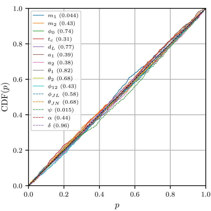
Results.—As a first test, we evaluate DINGO on data entirely consistent with the training distribution, i.e., simulated waveforms in stationary-Gaussian noise. This is an easier task than using observational data, which includes real signals in noise that is neither strictly stationary nor Gaussian, and therefore lies outside the training distribution. We sample posteriors from 1000 simulated data sets and construct a P–P plot (see Fig. 2). For each parameter, we compute the percentile score of the true value within its marginalized posterior, and then we plot the cumulative distribution function (CDF) of these scores. For true posteriors, the percentiles should be uniformly distributed, so the CDF should be diagonal. Kolmogorov-Smirnov test -values are indicated in the legend, with combined -value of 0.46. This shows that DINGO is performing properly on simulated data.
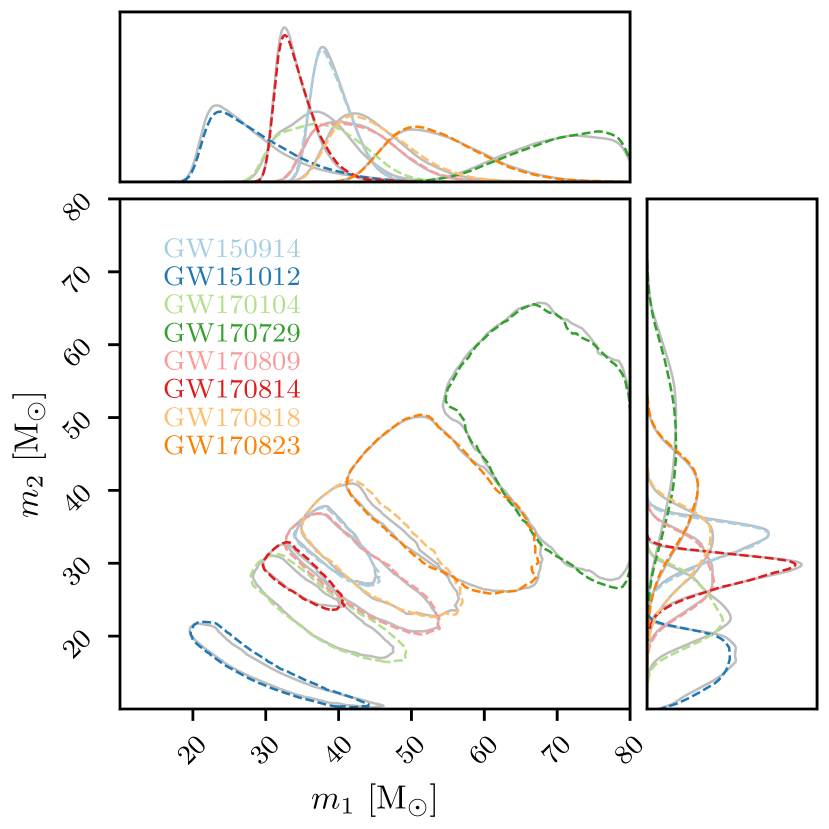
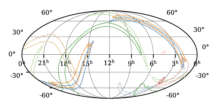
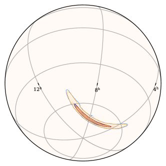
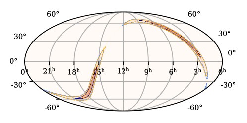
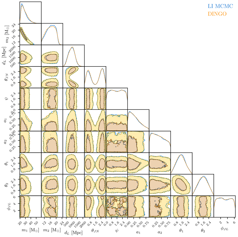
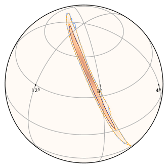
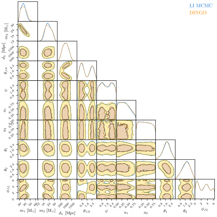
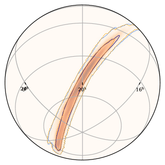
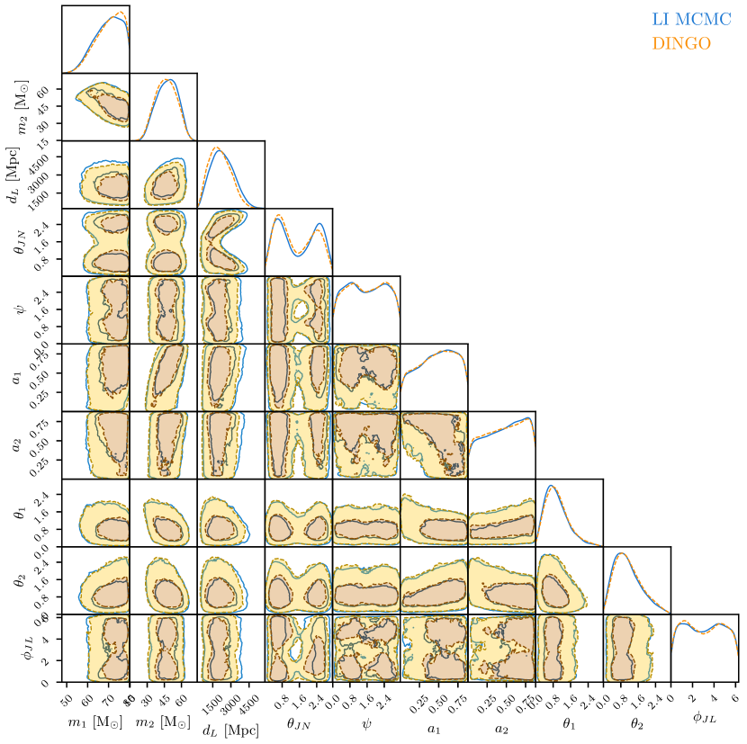
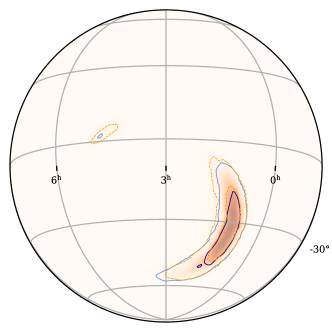
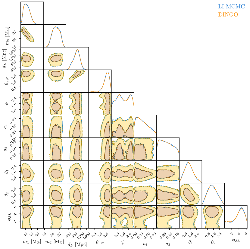
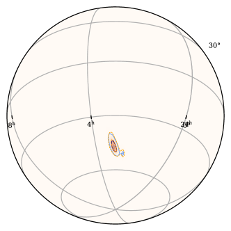
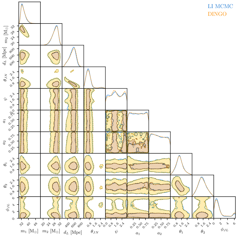
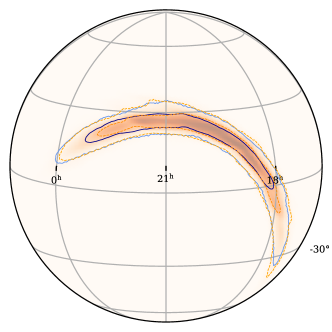
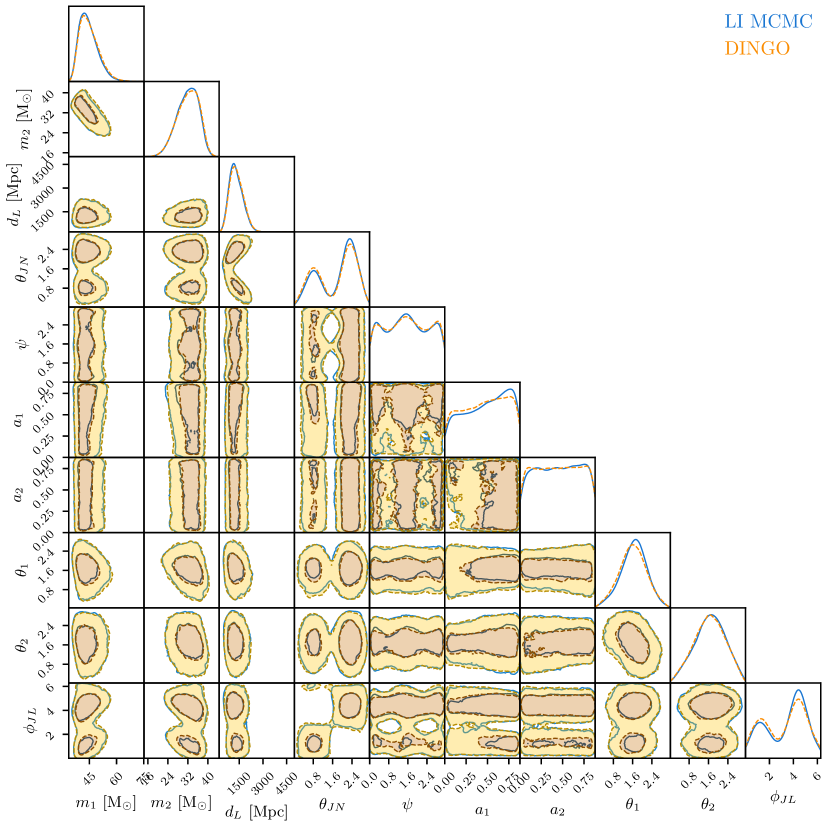
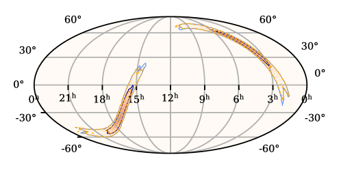
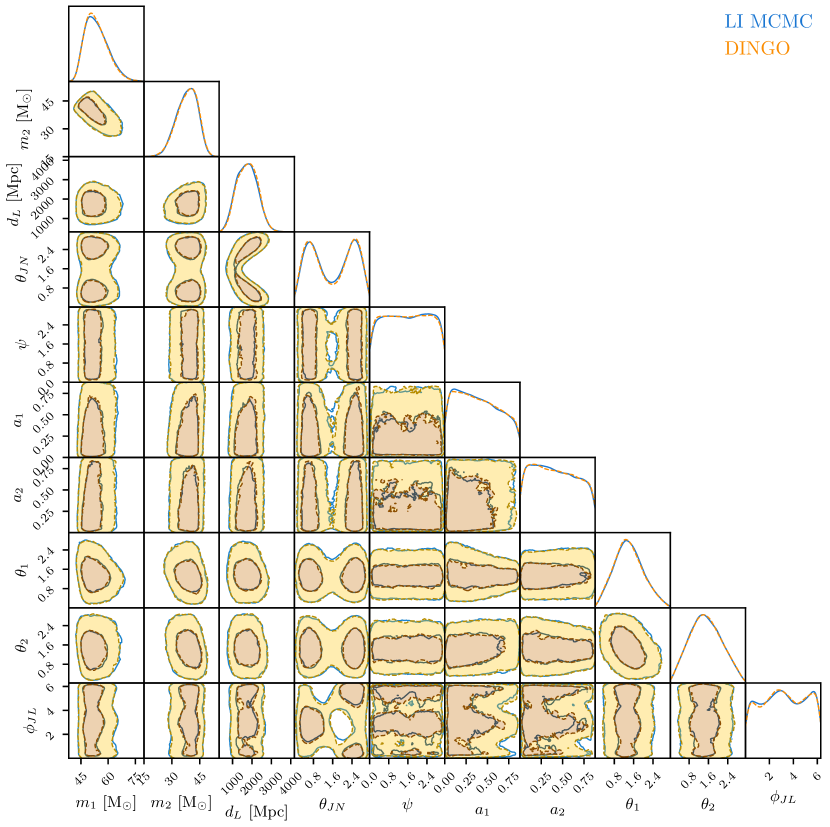
We now proceed to our main result, which is a demonstration of performance on real events. We perform inference on the eight GWTC-1 BBH events compatible with our prior, using both DINGO and LALInference MCMC. For DINGO, generation of 50,000 sample points with 30 GNPE iterations takes roughly 20 seconds. Comparisons of inferred component masses and sky position for all events show good agreement (see Fig. 3), including multimodality for the sky position. The one exception is GW170104, where the mass posterior is slightly flatter. Nevertheless, 90% credible intervals are in good agreement.
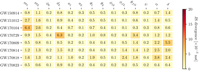
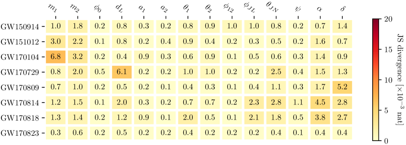
For quantitative comparisons, we compute the Jensen-Shannon divergence (JSD) [54] between DINGO and LALInference one-dimensional marginalized posteriors (see Fig. 4). This is a symmetric divergence that measures the difference between two probability distributions, with values ranging from 0 to nat. We find a mean JSD across all events and parameters of 0.0009 nat, which is slightly higher than the variation (0.0007 nat) found between LALInference runs with identical settings but different random seeds [19]. By comparing such LALInference runs, Ref. [19] also established a maximum JSD of 0.002 nat for indistinguishability; our results are approaching this threshold, with two events below for all parameters, and the others with one to three parameters above. The slight visible disagreement between mass posteriors for GW170104 is also reflected in larger JSDs. For comparison, we note that PSD variations (see Supplemental Material) and the choice of waveform model [19] both impact the JSD at a much higher level (0.02 nat). Additional comparisons between samplers, including posteriors for all events, are provided in the Supplemental Material.
Conclusions.—In this Letter, we introduced DINGO and applied it to perform extremely fast Bayesian parameter inference for gravitational waves observed by the LIGO and Virgo detectors. We analyzed eight GWTC-1 events, and showed excellent agreement with standard algorithms, with inference times reduced by factors of –. This was achieved by conditioning on the detector noise characteristics and making a number of architecture and algorithm improvements. The DINGO code is available at https://github.com/dingo-gw/dingo.
A critical component of DINGO is a new iterative algorithm—GNPE—to partially off-load the modeling of time translations from the neural network. Although convergence of GNPE may take 20 seconds, initial samples with slightly reduced accuracy can, however, be produced in just a few seconds by taking fewer iterations.
Going forward, the next steps are to extend the prior to include longer-duration binary neutron star signals [55] (for which rapid results are especially important to identify electromagnetic counterparts) and to extend to more physically-realistic waveform models, which include higher multipole modes and more accurate spin-precession effects [21]. Long and complex waveforms are much more expensive for standard algorithms, so the relative improvement in performance should be even more significant. If successful, this would also enable the routine use of the most physically-realistic waveforms, resulting in consistently reduced systematic errors. These extensions will likely require somewhat larger networks and improved data representation or compression.222Initial estimates based on a singular value decomposition [56] indicate that to accurately represent SEOBNRv4PHM BBH waveforms [21], the initial layers of our embedding network should be widened by a factor of roughly four. Assuming the same number of iterations and fixed hardware, the total training time would increase by about 35%. For binary neutron stars, adopting a frequency-dependent resolution [57, 58] would limit the expansion of the number of frequency bins to a factor of three.
Another natural extension would be to study signals without making the common stationary-Gaussian idealization for the detector noise during the training stage. For DINGO, performing inference with realistic noise is simply a matter of training with simulated signals injected into real noise realizations taken from detectors. Using real noise should lead to improved accuracy that is not possible using standard likelihood-based methods, and would serve as an excellent demonstration of the advantages of NPE. For real-time analysis, it will also be necessary to develop approaches to progressively retrain networks to keep pace with changing data distributions during an observing run, e.g., as detector sensitivity is improved. All of these enhancements, particularly the treatment of nonstationary noise, will be critical for extensions to future observatories such as LISA.
Deep-learning tools are now ready to analyze the vast majority of LIGO/Virgo events. In the past, the primary challenge has been in obtaining sufficiently accurate results, but with DINGO, we have now achieved this in a realistic context. Through planned future extensions, we expect that DINGO could become one of the leading approaches to gravitational-wave inference.
Acknowledgements.
Acknowledgments.—We thank S. Ossokine, M. Pürrer, C. Simpson and P. Züge for helpful discussions. This research has made use of data, software and/or web tools obtained from the Gravitational Wave Open Science Center (https://www.gw-openscience.org/ ), a service of LIGO Laboratory, the LIGO Scientific Collaboration and the Virgo Collaboration. LIGO Laboratory and Advanced LIGO are funded by the United States National Science Foundation (NSF) as well as the Science and Technology Facilities Council (STFC) of the United Kingdom, the Max-Planck-Society (MPS), and the State of Niedersachsen/Germany for support of the construction of Advanced LIGO and construction and operation of the GEO600 detector. Additional support for Advanced LIGO was provided by the Australian Research Council. Virgo is funded, through the European Gravitational Observatory (EGO), by the French Centre National de Recherche Scientifique (CNRS), the Italian Istituto Nazionale di Fisica Nucleare (INFN) and the Dutch Nikhef, with contributions by institutions from Belgium, Germany, Greece, Hungary, Ireland, Japan, Monaco, Poland, Portugal, Spain. This material is based upon work supported by NSF’s LIGO Laboratory which is a major facility fully funded by the National Science Foundation. M.D. thanks the Hector Fellow Academy for support. J.H.M. and B.S. are members of the MLCoE, EXC number 2064/1 – Project number 390727645. We usePyTorch [59] and nflows [60]
for the implementation of our neural networks. The plots are generated
with matplotlib [61],
ChainConsumer [62] and
ligo.skymap [63].
References
- Abbott et al. [2016] B. Abbott et al. (LIGO Scientific, Virgo), Observation of Gravitational Waves from a Binary Black Hole Merger, Phys. Rev. Lett. 116, 061102 (2016), arXiv:1602.03837 [gr-qc] .
- Abbott et al. [2021a] R. Abbott et al. (LIGO Scientific, Virgo), Tests of general relativity with binary black holes from the second LIGO-Virgo gravitational-wave transient catalog, Phys. Rev. D 103, 122002 (2021a), arXiv:2010.14529 [gr-qc] .
- Abbott et al. [2018] B. P. Abbott et al. (LIGO Scientific, Virgo), GW170817: Measurements of neutron star radii and equation of state, Phys. Rev. Lett. 121, 161101 (2018), arXiv:1805.11581 [gr-qc] .
- Abbott et al. [2021b] B. P. Abbott et al. (LIGO Scientific, Virgo), A Gravitational-wave Measurement of the Hubble Constant Following the Second Observing Run of Advanced LIGO and Virgo, Astrophys. J. 909, 218 (2021b), arXiv:1908.06060 [astro-ph.CO] .
- Abbott et al. [2021c] R. Abbott et al. (LIGO Scientific, Virgo), Population Properties of Compact Objects from the Second LIGO-Virgo Gravitational-Wave Transient Catalog, Astrophys. J. Lett. 913, L7 (2021c), arXiv:2010.14533 [astro-ph.HE] .
- Aasi et al. [2015] J. Aasi et al. (LIGO Scientific), Advanced LIGO, Class. Quant. Grav. 32, 074001 (2015), arXiv:1411.4547 [gr-qc] .
- Acernese et al. [2015] F. Acernese et al. (VIRGO), Advanced Virgo: a second-generation interferometric gravitational wave detector, Class. Quant. Grav. 32, 024001 (2015), arXiv:1408.3978 [gr-qc] .
- Abbott et al. [2019] B. P. Abbott et al. (LIGO Scientific, Virgo), GWTC-1: A Gravitational-Wave Transient Catalog of Compact Binary Mergers Observed by LIGO and Virgo during the First and Second Observing Runs, Phys. Rev. X 9, 031040 (2019), arXiv:1811.12907 [astro-ph.HE] .
- Abbott et al. [2021d] R. Abbott et al. (LIGO Scientific, Virgo), GWTC-2: Compact Binary Coalescences Observed by LIGO and Virgo During the First Half of the Third Observing Run, Phys. Rev. X 11, 021053 (2021d), arXiv:2010.14527 [gr-qc] .
- Abbott et al. [2020a] B. P. Abbott et al. (KAGRA, LIGO Scientific, Virgo), Prospects for observing and localizing gravitational-wave transients with Advanced LIGO, Advanced Virgo and KAGRA, Living Rev. Rel. 23, 3 (2020a).
- Abbott et al. [2020b] B. P. Abbott et al. (LIGO Scientific, Virgo), A guide to LIGO–Virgo detector noise and extraction of transient gravitational-wave signals, Class. Quant. Grav. 37, 055002 (2020b), arXiv:1908.11170 [gr-qc] .
- Buonanno and Damour [1999] A. Buonanno and T. Damour, Effective one-body approach to general relativistic two-body dynamics, Phys. Rev. D 59, 084006 (1999), arXiv:gr-qc/9811091 .
- Bohé et al. [2017] A. Bohé et al., Improved effective-one-body model of spinning, nonprecessing binary black holes for the era of gravitational-wave astrophysics with advanced detectors, Phys. Rev. D 95, 044028 (2017), arXiv:1611.03703 [gr-qc] .
- Varma et al. [2019] V. Varma, S. E. Field, M. A. Scheel, J. Blackman, L. E. Kidder, and H. P. Pfeiffer, Surrogate model of hybridized numerical relativity binary black hole waveforms, Phys. Rev. D 99, 064045 (2019), arXiv:1812.07865 [gr-qc] .
- Pürrer [2016] M. Pürrer, Frequency domain reduced order model of aligned-spin effective-one-body waveforms with generic mass-ratios and spins, Phys. Rev. D 93, 064041 (2016), arXiv:1512.02248 [gr-qc] .
- Khan et al. [2016] S. Khan, S. Husa, M. Hannam, F. Ohme, M. Pürrer, X. Jimńez Forteza, and A. Bohé, Frequency-domain gravitational waves from nonprecessing black-hole binaries. II. A phenomenological model for the advanced detector era, Phys. Rev. D93, 044007 (2016), arXiv:1508.07253 [gr-qc] .
- Veitch et al. [2015] J. Veitch et al., Parameter estimation for compact binaries with ground-based gravitational-wave observations using the LALInference software library, Phys. Rev. D91, 042003 (2015), arXiv:1409.7215 [gr-qc] .
- Ashton et al. [2019] G. Ashton et al., BILBY: A user-friendly Bayesian inference library for gravitational-wave astronomy, Astrophys. J. Suppl. 241, 27 (2019), arXiv:1811.02042 [astro-ph.IM] .
- Romero-Shaw et al. [2020] I. M. Romero-Shaw et al., Bayesian inference for compact binary coalescences with bilby: validation and application to the first LIGO–Virgo gravitational-wave transient catalogue, Mon. Not. Roy. Astron. Soc. 499, 3295 (2020), arXiv:2006.00714 [astro-ph.IM] .
- Speagle [2020] J. S. Speagle, dynesty: a dynamic nested sampling package for estimating bayesian posteriors and evidences, Monthly Notices of the Royal Astronomical Society 493, 3132–3158 (2020), arXiv:1904.02180 [astro-ph.IM] .
- Ossokine et al. [2020] S. Ossokine et al., Multipolar Effective-One-Body Waveforms for Precessing Binary Black Holes: Construction and Validation, Phys. Rev. D 102, 044055 (2020), arXiv:2004.09442 [gr-qc] .
- Abbott et al. [2017a] B. P. Abbott et al. (LIGO Scientific, Virgo, Fermi GBM, INTEGRAL, IceCube, AstroSat Cadmium Zinc Telluride Imager Team, IPN, Insight-Hxmt, ANTARES, Swift, AGILE Team, 1M2H Team, Dark Energy Camera GW-EM, DES, DLT40, GRAWITA, Fermi-LAT, ATCA, ASKAP, Las Cumbres Observatory Group, OzGrav, DWF (Deeper Wider Faster Program), AST3, CAASTRO, VINROUGE, MASTER, J-GEM, GROWTH, JAGWAR, CaltechNRAO, TTU-NRAO, NuSTAR, Pan-STARRS, MAXI Team, TZAC Consortium, KU, Nordic Optical Telescope, ePESSTO, GROND, Texas Tech University, SALT Group, TOROS, BOOTES, MWA, CALET, IKI-GW Follow-up, H.E.S.S., LOFAR, LWA, HAWC, Pierre Auger, ALMA, Euro VLBI Team, Pi of Sky, Chandra Team at McGill University, DFN, ATLAS Telescopes, High Time Resolution Universe Survey, RIMAS, RATIR, SKA South Africa/MeerKAT), Multi-messenger Observations of a Binary Neutron Star Merger, Astrophys. J. Lett. 848, L12 (2017a), arXiv:1710.05833 [astro-ph.HE] .
- Pratten et al. [2020] G. Pratten, S. Husa, C. Garcia-Quiros, M. Colleoni, A. Ramos-Buades, H. Estelles, and R. Jaume, Setting the cornerstone for a family of models for gravitational waves from compact binaries: The dominant harmonic for nonprecessing quasicircular black holes, Phys. Rev. D 102, 064001 (2020), arXiv:2001.11412 [gr-qc] .
- Pratten et al. [2021] G. Pratten et al., Computationally efficient models for the dominant and subdominant harmonic modes of precessing binary black holes, Phys. Rev. D 103, 104056 (2021), arXiv:2004.06503 [gr-qc] .
- Singer and Price [2016] L. P. Singer and L. R. Price, Rapid Bayesian position reconstruction for gravitational-wave transients, Phys. Rev. D 93, 024013 (2016), arXiv:1508.03634 [gr-qc] .
- Lange et al. [2018] J. Lange, R. O’Shaughnessy, and M. Rizzo, Rapid and accurate parameter inference for coalescing, precessing compact binaries, (2018), arXiv:1805.10457 [gr-qc] .
- Cornish [2021] N. J. Cornish, Rapid and Robust Parameter Inference for Binary Mergers, Phys. Rev. D 103, 104057 (2021), arXiv:2101.01188 [gr-qc] .
- Papamakarios and Murray [2016] G. Papamakarios and I. Murray, Fast -free inference of simulation models with bayesian conditional density estimation (2016), arXiv:1605.06376 [stat.ML] .
- Lueckmann et al. [2017] J.-M. Lueckmann, P. J. Gonçalves, G. Bassetto, K. Öcal, M. Nonnenmacher, and J. H. Macke, Flexible statistical inference for mechanistic models of neural dynamics, in Proceedings of the 31st International Conference on Neural Information Processing Systems (2017) pp. 1289–1299.
- Greenberg et al. [2019] D. Greenberg, M. Nonnenmacher, and J. Macke, Automatic posterior transformation for likelihood-free inference, in International Conference on Machine Learning (PMLR, 2019) pp. 2404–2414.
- Cranmer et al. [2020] K. Cranmer, J. Brehmer, and G. Louppe, The frontier of simulation-based inference, Proc. Nat. Acad. Sci. 117, 30055 (2020), arXiv:1911.01429 [stat.ML] .
- Gabbard et al. [2019] H. Gabbard, C. Messenger, I. S. Heng, F. Tonolini, and R. Murray-Smith, Bayesian parameter estimation using conditional variational autoencoders for gravitational-wave astronomy (2019), arXiv:1909.06296 [astro-ph.IM] .
- Chua and Vallisneri [2020] A. J. K. Chua and M. Vallisneri, Learning Bayesian posteriors with neural networks for gravitational-wave inference, Phys. Rev. Lett. 124, 041102 (2020), arXiv:1909.05966 [gr-qc] .
- Chatterjee et al. [2019] C. Chatterjee, L. Wen, K. Vinsen, M. Kovalam, and A. Datta, Using Deep Learning to Localize Gravitational Wave Sources, Phys. Rev. D 100, 103025 (2019), arXiv:1909.06367 [astro-ph.IM] .
- Green et al. [2020] S. R. Green, C. Simpson, and J. Gair, Gravitational-wave parameter estimation with autoregressive neural network flows, Phys. Rev. D 102, 104057 (2020), arXiv:2002.07656 [astro-ph.IM] .
- Green and Gair [2021] S. R. Green and J. Gair, Complete parameter inference for GW150914 using deep learning, Mach. Learn. Sci. Tech. 2, 03LT01 (2021), arXiv:2008.03312 [astro-ph.IM] .
- Delaunoy et al. [2020] A. Delaunoy, A. Wehenkel, T. Hinderer, S. Nissanke, C. Weniger, A. R. Williamson, and G. Louppe, Lightning-Fast Gravitational Wave Parameter Inference through Neural Amortization, (2020), arXiv:2010.12931 [astro-ph.IM] .
- Krastev et al. [2021] P. G. Krastev, K. Gill, V. A. Villar, and E. Berger, Detection and Parameter Estimation of Gravitational Waves from Binary Neutron-Star Mergers in Real LIGO Data using Deep Learning, Phys. Lett. B 815, 136161 (2021), arXiv:2012.13101 [astro-ph.IM] .
- Shen et al. [2021] H. Shen, E. A. Huerta, E. O’Shea, P. Kumar, and Z. Zhao, Statistically-informed deep learning for gravitational wave parameter estimation, (2021), arXiv:1903.01998v3 [gr-qc] .
- Cuoco et al. [2020] E. Cuoco, J. Powell, M. Cavaglià, K. Ackley, M. Bejger, C. Chatterjee, M. Coughlin, S. Coughlin, P. Easter, R. Essick, et al., Enhancing gravitational-wave science with machine learning, Machine Learning: Science and Technology 2, 011002 (2020), arXiv:2005.03745 [astro-ph.HE] .
- Farr et al. [2014] B. Farr, E. Ochsner, W. M. Farr, and R. O’Shaughnessy, A more effective coordinate system for parameter estimation of precessing compact binaries from gravitational waves, Phys. Rev. D 90, 024018 (2014), arXiv:1404.7070 [gr-qc] .
- Rezende and Mohamed [2015] D. Rezende and S. Mohamed, Variational inference with normalizing flows, in International Conference on Machine Learning (2015) pp. 1530–1538, 1505.05770 [stat.ML] .
- Kingma et al. [2016] D. P. Kingma, T. Salimans, R. Jozefowicz, X. Chen, I. Sutskever, and M. Welling, Improved variational inference with inverse autoregressive flow, in Advances in neural information processing systems (2016) pp. 4743–4751, arXiv:1606.04934 [cs.LG] .
- Papamakarios et al. [2017] G. Papamakarios, T. Pavlakou, and I. Murray, Masked autoregressive flow for density estimation, in Advances in Neural Information Processing Systems (2017) pp. 2338–2347, arXiv:1705.07057 [stat.ML] .
- Durkan et al. [2019] C. Durkan, A. Bekasov, I. Murray, and G. Papamakarios, Neural spline flows, in Advances in Neural Information Processing Systems (2019) pp. 7509–7520, arXiv:1906.04032 [stat.ML] .
- Littenberg and Cornish [2015] T. B. Littenberg and N. J. Cornish, Bayesian inference for spectral estimation of gravitational wave detector noise, Phys. Rev. D 91, 084034 (2015), arXiv:1410.3852 [gr-qc] .
- He et al. [2015] K. He, X. Zhang, S. Ren, and J. Sun, Deep residual learning for image recognition (2015), arXiv:1512.03385 [cs.CV] .
- Dax et al. [2022] M. Dax, S. R. Green, J. Gair, M. Deistler, B. Schölkopf, and J. H. Macke, Group equivariant neural posterior estimation, International Conference on Learning Representations, (2022), arXiv:2111.13139 [cs.LG] .
- Goodfellow et al. [2016] I. Goodfellow, Y. Bengio, and A. Courville, Deep Learning (MIT Press, 2016) http://www.deeplearningbook.org.
- Kingma and Ba [2014] D. P. Kingma and J. Ba, Adam: A Method for Stochastic Optimization, (2014), arXiv:1412.6980 [cs.LG] .
- Abbott et al. [2021e] R. Abbott et al. (LIGO Scientific, Virgo), Open data from the first and second observing runs of Advanced LIGO and Advanced Virgo, SoftwareX 13, 100658 (2021e), arXiv:1912.11716 [gr-qc] .
- Hannam et al. [2014] M. Hannam, P. Schmidt, A. Bohé, L. Haegel, S. Husa, F. Ohme, G. Pratten, and M. Pürrer, Simple Model of Complete Precessing Black-Hole-Binary Gravitational Waveforms, Phys. Rev. Lett. 113, 151101 (2014), arXiv:1308.3271 [gr-qc] .
- Bohé et al. [2016] A. Bohé, M. Hannam, S. Husa, F. Ohme, M. Pürrer, and P. Schmidt, PhenomPv2 – technical notes for the LAL implementation, LIGO Technical Document, LIGO-T1500602-v4 (2016).
- Lin [1991] J. Lin, Divergence measures based on the shannon entropy, IEEE Transactions on Information theory 37, 145 (1991).
- Abbott et al. [2017b] B. P. Abbott et al. (LIGO Scientific, Virgo), GW170817: Observation of Gravitational Waves from a Binary Neutron Star Inspiral, Phys. Rev. Lett. 119, 161101 (2017b), arXiv:1710.05832 [gr-qc] .
- Cannon et al. [2010] K. Cannon, A. Chapman, C. Hanna, D. Keppel, A. C. Searle, and A. J. Weinstein, Singular value decomposition applied to compact binary coalescence gravitational-wave signals, Phys. Rev. D 82, 044025 (2010), arXiv:1005.0012 [gr-qc] .
- Vinciguerra et al. [2017] S. Vinciguerra, J. Veitch, and I. Mandel, Accelerating gravitational wave parameter estimation with multi-band template interpolation, Class. Quant. Grav. 34, 115006 (2017), arXiv:1703.02062 [gr-qc] .
- Cannon et al. [2012] K. Cannon et al., Toward Early-Warning Detection of Gravitational Waves from Compact Binary Coalescence, Astrophys. J. 748, 136 (2012), arXiv:1107.2665 [astro-ph.IM] .
- Paszke et al. [2019] A. Paszke, S. Gross, F. Massa, A. Lerer, J. Bradbury, G. Chanan, T. Killeen, Z. Lin, N. Gimelshein, L. Antiga, A. Desmaison, A. Kopf, E. Yang, Z. DeVito, M. Raison, A. Tejani, S. Chilamkurthy, B. Steiner, L. Fang, J. Bai, and S. Chintala, Pytorch: An imperative style, high-performance deep learning library, in Advances in Neural Information Processing Systems 32 (Curran Associates, Inc., 2019) pp. 8024–8035.
- Durkan et al. [2020] C. Durkan, A. Bekasov, I. Murray, and G. Papamakarios, nflows: normalizing flows in PyTorch (2020).
- Hunter [2007] J. D. Hunter, Matplotlib: A 2d graphics environment, Computing in Science & Engineering 9, 90 (2007).
- Hinton [2016] S. R. Hinton, ChainConsumer, The Journal of Open Source Software 1, 00045 (2016).
- Singer [2020] L. Singer, ligo.skymap, https://lscsoft.docs.ligo.org/ligo.skymap/ (2020).
Supplemental Material
I Training data
We perform inference over the full 15D parameter space for quasicircular binary black holes, which includes detector-frame component masses , , time of coalescence at geocenter , reference phase , sky position (right ascension and declination ), luminosity distance , inclination angle , spin magnitudes , , tilt angles , , other spin angles , [41], and polarization angle . Priors are taken to be the same as in Ref. [36]: standard over all angles, and uniform in all other parameters, with , , , and . We found that it was difficult to train a neural network for accurate inference over the entire relevant range of luminosity distance, so we partition the prior as shown in Tab. 1. To perturb the signal coalescence times for GNPE ,we use a uniform kernel in the range .
| Observing run | Detectors | Distance range [Mpc] |
|---|---|---|
| O1 | HL | [100, 2000] |
| O2 | HL | [100, 2000] |
| [100, 6000] | ||
| HLV | [100, 1000] |
Training data consist of labeled strain data sets and associated noise power spectral densities . To construct the data sets, we first draw samples from the prior, . This is done in two stages as in Ref. [36]: first, intrinsic parameters are sampled ahead of training, and waveforms are generated and saved based on these; second, extrinsic parameters are sampled during training and applied to the waveforms, since this involves simple transformations. For our purposes, intrinsic parameters consist of and extrinsic parameters are .
Each strain data set consists of a waveform with additive stationary Gaussian noise, . This is represented in frequency domain, with , , and , corresponding to a duration of 8 s. Waveforms are generated using the IMRPhenomPv2 frequency-domain model [52, 16, 53], which is fast (so that comparisons against standard samplers are feasible) and also includes spin-precession effects. We save intrinsic waveforms to disk in an SVD representation, which is accurate to a mismatch of for the th percentile of the data. Noise realizations are generated during training, after first sampling an associated PSD, i.e., , . We construct training sets based on sets of intrinsic parameters, but by sampling extrinsic parameters and noise realizations during training, the effective size of the training set is infinite in these dimensions.
To construct the empirical PSD distributions , we
estimate PSDs using noise data from each observing run. Using
BURST_CAT2 data from GWOSC [51], we identify
stretches of at least 1024 s in duration that do not overlap with
events. Each PSD is estimated by taking a 1024 s stretch of data,
dividing this into non-overlapping 8 s subintervals, and using the
Welch “median-average” method to average PSDs estimated on each of
these [17]. We use a Tukey window with a roll-off of
0.4 s. For inference, we use the same construction to estimate the PSD
from detector data just prior to an event. The number of PSDs obtained
for each observing run is given in Tab. 2.
| Observing run | Detector | Number of PSDs |
| O1 | H | 2444 |
| L | 2414 | |
| O2 | H | 4670 |
| L | 3873 | |
| V | 864 |
II Neural network
There are two main components to our conditional density-estimation neural network, the embedding network for compressing data to a sufficiently small number of features, and the normalizing flow, which produces the Bayesian posterior from these features.
II.1 Embedding network
For each of the two or three detectors, the embedding network takes as input the real and imaginary parts of the whitened frequency-domain strain data, as well as the inverse amplitude spectral density (ASD). This results in 24,096 inputs per detector. We provide the inverse ASD rather than the PSD because of the more numerically stable behavior of spectral lines. We scale the ASD with a constant factor of .
The first embedding layer is a linear mapping that serves to drastically reduce the number of dimensions. This is initialized based on a singular value decomposition (SVD) to provide an inductive bias to facilitate training. The strain data are initially projected onto the first (complex) singular vectors, defined based on a set of 50,000 signal waveforms drawn from the prior. The inverse ASDs are likewise mapped to complex numbers, which are added to the projected strain; this projection is initialized to 0. After this initial layer, the data has therefore been projected onto (real) features (i.e., either 800 or 1200 components, depending on the number of detectors). There is no nonlinear activation following this layer.
Following the SVD layer is a fully-connected residual network. This consists of a sequence of two-layer residual blocks; prior to each linear mapping are batch normalization layers and ELU activation functions. We take six blocks each of 1024, 512, 256, and 128 hidden dimensions, resulting in a total of 48 hidden layers in the residual network.
II.2 Normalizing flow
Our normalizing flow is very similar to that of [36]. This consists of a sequence of coupling transforms, each of which transforms half of the components of a sample element-wise based on the context information and the values of the untransformed components. We use a rational-quadratic spline coupling transform [45], with the same parameters as in [36], except for the number of residual blocks, which is reduced from 10 to 5. Between the coupling transforms, the ordering of the sample components is randomized to ensure all components are sufficiently transformed by the sequence of transforms. We also increase the total number of coupling transforms to 30 from 15 in [36]. The flow therefore consists of 300 hidden layers. In total, the embedding network and the flow combined have learnable parameters for and for .
The context information for the flow consists of the 128 features output from the embedding network, as well as the two or three perturbed detector coalescence times .
We also train a neural network to provide an initial estimate for , which is used as a starting point for the iterative GNPE algorithm. This does not require as context, but otherwise has the same form as the main network.
II.3 Training
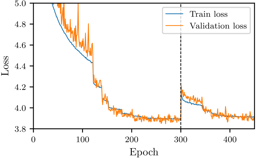
Training consists of two stages, an initial pretraining stage and a fine-tuning stage. During the pretraining stage, the SVD layer is frozen, and all noise realizations are drawn from an average PSD for the observing run and detector. This is designed to simplify early-stage training. During the fine-tuning stage, the SVD layer is unfrozen, and PSDs are randomly drawn from the empirical distribution, and noise realizations are drawn from these.
Our networks are trained for 300 epochs of pretraining and 150 epochs of fine tuning with a batch size of . We use the Adam optimizer [50]. We begin training with learning rates of and in the pretraining and finetuning stages, respectively, and decrease the learning rate by a factor of when the validation loss has not improved in the previous 10 epochs. For three detectors, we reduce the batch size to and the initial learning rates to and due to memory limitations. As shown in Fig. 5, the loss jumps at the beginning of the fine-tuning stage. This occurs because the distribution of training data becomes much broader with the inclusion of varying noise PSDs. The final loss at the end of fine tuning is just above the pretraining loss, which indicates that the network has learned to process the varying PSDs to the same performance level of the fixed pretraining PSD. During training, we reserve 2% of the training set for validation to check for overfitting. Since the training and validation loss are in close agreement in Fig. 5 we conclude that overfitting is minimal. Training 450 epochs with a batch size of takes roughly 10 days on a single NVIDIA A100 GPU.333With an NVIDIA V100 GPU (16GB) training takes 16-18 days, and inference roughly a minute per event (rather than 20 seconds).
III Effect of PSD
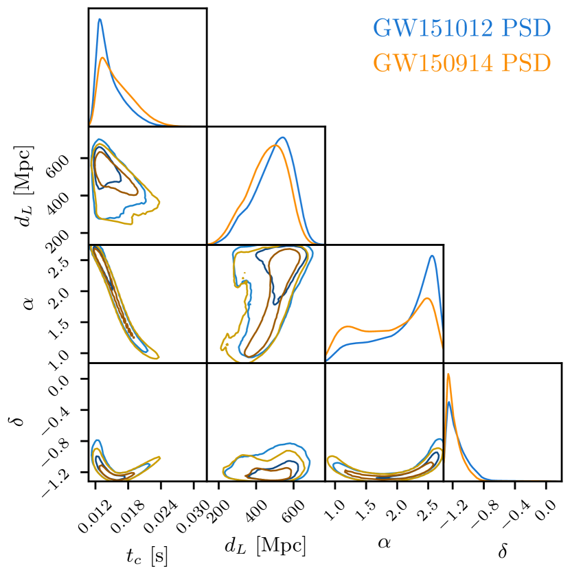
To give a sense of the size of the effect of the PSD on the posterior, we perform inference on GW150914, where we whiten the strain data with the correct PSD, but provide instead the PSD for GW151012 as context to the neural network. This gives a mean JSD across all parameters of 0.005 nat and a maximum JSD of 0.030 nat when compared against the DINGO result using the correct PSD. Both of these numbers significantly exceed the JSDs between DINGO and LALInference runs for all events [largest mean JSD: 0.001 nat (GW170729); largest maximum JSD: 0.006 nat (GW170104, )]. This demonstrates that conditioning the neural network on the PSD is required at the level of accuracy we achieve in this study.
The worst performing parameters with the incorrect PSD are , , , and , which have a mean JSD of 0.020 nat (see Fig. 6). These results are consistent with the expectation that the main effect due to using the wrong PSD is to cause a change in the inferred amplitude of the signal in each detector: becomes biased due to the overall amplitude being off, whereas sky position and become biased from relative incorrect amplitudes in the two detectors.
IV Comparisons against standard samplers
| Event | ||||
|---|---|---|---|---|
| GW150914 | ||||
| GW151012 | ||||
| GW170104 | ||||
| GW170729 | ||||
| GW170809 | ||||
| GW170814 | ||||
| GW170818 | ||||
| GW170823 | ||||
We compare our results against LALInference [17] with MCMC and nested sampling algorithms, and with Bilby [18, 19] with the dynesty [20] nested sampling algorithm. To compare as closely as possible with DINGO, we use the same data conditioning for strain data and PSDs. However, we sample in chirp mass and mass ratio instead of component masses, since this simplifies the form of the posterior and improves convergence. We also sample sky position in the detector-based azimuth/zenith reference frame rather than the sky frame for Bilby. This also simplifies the form of the posterior to improve sampling [19].
With standard samplers it is possible to analytically marginalize over
some parameters to reduce the dimensionality of the space. This
improves sampling performance, with the marginalized parameters
reconstructed in post-processing. For LALInference, we marginalize
over time of coalescence, and with Bilby we marginalize over time,
distance, and phase. Phase marginalization is only valid in the
absence of precession, but we had difficulty obtaining converged
results without it. For IMRPhenomPv2 waveforms, this should not lead
to a significant difference, but it should be kept in mind. For Bilby,
we use nlive=4000 and nact=50.
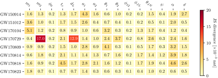
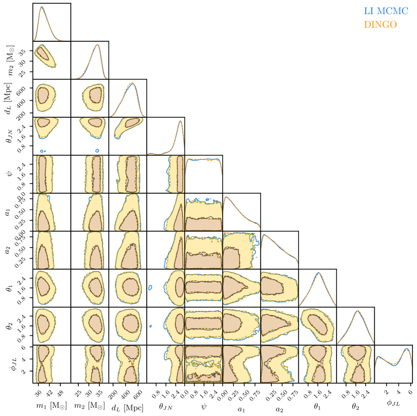
We find closest agreement with LALInference MCMC, which is what we report in the main text, and is displayed on all posterior plots. For completeness we include in Fig. 7 comparisons against LALInference nested sampling and Bilby with phase marginalization. In general, when using phase marginalization, spin and sky position are less well recovered, as were some events. To give a sense of how JSD values translate into parameter estimates, we provide 90% credible intervals in Tab. 3, which are all in extremely close agreement.
Deviations between posteriors obtained from DINGO and standard samplers are associated with multiple sources of error. Firstly, imperfect training of DINGO can lead to inaccurate results. Indeed, training the neural networks is challenging due to the high dimensionality of the input data to this inference problem, which inspired us to adopt the GNPE method [48] to improve convergence. While the P–P plot in Fig. 2 of the main text suggests that our networks are well converged, small deviations between posteriors for real events could arise due to the networks not being fully converged. Secondly, even the well-established standard samplers do not produce perfect posterior samples. The mean JSD between LALInference runs with identical settings but different random seeds is a factor 3.5 higher than that expected for samples from identical distributions (see Fig. 7 for details). Thirdly, perfect agreement between (ideal implementations of) DINGO and standard samplers is only expected for data consistent with the training distribution. In reality, however, where the noise is neither perfectly stationary nor Gaussian, the measured data is slightly out-of-distribution. In those cases, there is no theoretical guarantee that DINGO extrapolates to this data in the same way as standard samplers. However, as stated in the conclusion, DINGO is not limited to stationary Gaussian noise, and we plan to lift this assumption in future work.
In the remainder of this section, we include 1D and 2D marginalized posteriors for all nontrivial parameters for all events. All DINGO posteriors are produced with 50,000 samples, except for the skymaps, which use 10,000. LALInference posteriors use all samples produced with the given sampler settings, typically of order 30,000–50,000.
rc.95in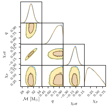 \stackinsetc-.5int-2in
 \cprotect
rc.95in \stackinsetct-2in
 \cprotect
rc.95in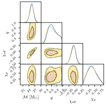 \stackinsetc-.5int-2in
 \cprotect
rc.95in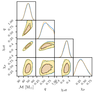 \stackinsetc-.5int-2in
 \cprotect
rc.95in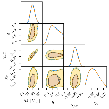 \stackinsetc-.5int-2in
 \cprotect
rc.95in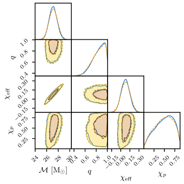 \stackinsetc-.5int-2in
 \cprotect
rc.95in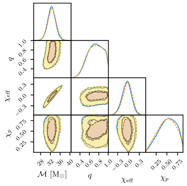 \stackinsetc-.5int-2in
 \cprotect
rc.95in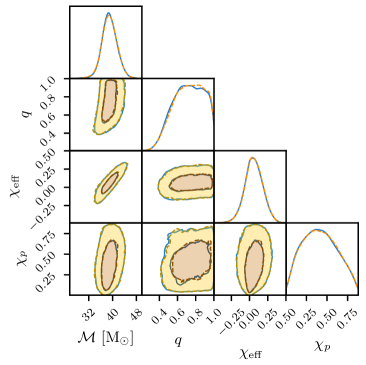 \stackinsetct-2in
 \cprotect