Ensemble photometric redshifts

Abstract

Upcoming imaging surveys, such as LSST, will provide an unprecedented view of the Universe, but with limited resolution along the line-of-sight. Common ways to increase resolution in the third dimension, and reduce misclassifications, include observing a wider wavelength range and/or combining the broad-band imaging with higher spectral resolution data. The challenge with these approaches is matching the depth of these ancillary data with the original imaging survey. However, while a full 3D map is required for some science, there are many situations where only the statistical distribution of objects ($dN/dz$) in the line-of-sight direction is needed. In such situations, there is no need to measure the fluxes of individual objects in all of the surveys. Rather a stacking procedure can be used to perform an “ensemble photo-$z$”. We show how a shallow, higher spectral resolution survey can be used to measure $dN/dz$ for stacks of galaxies which coincide in a deeper, lower resolution survey. The galaxies in the deeper survey do not even need to appear individually in the shallow survey. We give a toy model example to illustrate tradeoffs and considerations for applying this method. This approach will allow deep imaging surveys to leverage the high resolution of spectroscopic and narrow/medium band surveys underway, even when the latter do not have the same reach to high redshift.

1 Introduction

The Large Synoptic Survey Telescope (LSST) will be one of the key astronomical facilities of the next decade. It will allow us to map large areas of sky with unprecedented depth in six optical pass bands ($ugrizY$). The science enabled by this facility will be revolutionary (e.g. LSST Science Collaboration et al., 2009). Fully exploiting these deep sky maps will require information on the redshifts of the objects. A redshift estimate can be obtained directly from the photometry (a “photo-$z$”), but such redshifts are relatively poor and can be difficult to obtain for some types of galaxies (e.g. see Hildebrandt et al., 2010; Dahlen et al., 2013; Sánchez et al., 2014; Rau et al., 2015, for recent reviews). Of particular interest here is the use of LSST for studies of large-scale structure, which heavily impacts cosmology and fundamental physics. For such problems the addition of high-quality redshift information is critical (e.g. Newman et al., 2015).

One can seek to obtain redshifts for individual galaxies or the redshift distribution for a particularly interesting subsample. The latter will be the topic of this paper. Knowledge of $dN/dz$ for a sample can be used to invert a measured 2D correlation function into a 3D correlation function (Limber, 1953, 1954) or to interpret the results of a cosmic shear experiment (Hoekstra & Jain, 2008). The most natural method for obtaining $dN/dz$ is to ‘stack’ the photo-$z$s (or the redshift PDFs) of the galaxies making up the sample. Another method is to use the fact that objects which are close on the sky are also likely to be close in redshift. There is a long history of using such “cross-correlation” techniques to determine $dN/dz$ (Seldner & Peebles, 1979; Phillipps, 1985; Phillipps & Shanks, 1987; Padmanabhan et al., 2007; Ho et al., 2008; Erben et al., 2009; Benjamin et al., 2010, 2013; Newman, 2008; Matthews & Newman, 2010; Schulz, 2010; McQuinn & White, 2013; Matthews et al., 2013; Ménard et al., 2013; Schmidt et al., 2013; Rahman et al., 2015; Choi et al., 2016) and such methods can perform very well.

Unfortunately, degeneracies in color-type-redshift space are a notorious problem with traditional photo-$z$ methods, especially when restricted to broad-band optical photometry. In this case, galaxies of different types/redshifts can have the same colors (Benítez, 2000) and thus are indistinguishable. These degeneracies are often easily broken by adding photometry in IR-bands, appropriately chosen narrow-band imaging or low-redshift spectroscopy. However, it is often challenging to match the depths of these additional data with the original imaging catalog, especially for wide imaging surveys. The key idea in this paper is the realization that in order to determine redshift distributions, it is not necessary to detect individual sources in these additional data. For large enough samples, a “stacked” measurement can constrain the redshift distribution, even if the individual galaxies are all below the detection threshold. We dub this idea “ensemble photo-$z$’s”.

This idea is of particular interest since a number of narrow-band imaging/low resolution spectroscopy large-scale surveys are independently motivated. For instance, SPHEREx (Spectro-Photometer for the History of the Universe, Epoch of Reionization, and Ices Explorer) is an all-sky spectroscopic survey satellite which will obtain $R=35-41$ spectra for $0.75<\lambda<3.82\mu$m and $R=110-130$ spectra for $3.82<\lambda<5.0\mu$m, for a total of 96 bands, for every 6.2 arc second pixel over the entire-sky (Doré et al., 2014). J-PAS (Javalambre Physics of the Accelerating Universe Astrophysical Survey) will cover 8000 deg² using 56 narrow band filters in the optical (Benitez et al., 2014). PAUS (Physics of the Accelerating Universe Survey) will provide a 100 deg² 3D maps using 40 narrow band filters covering $4500<\lambda<8500~{}\AA$ on the William Herschel Telescope (Castander et al., 2012). ALHAMBRA (Advanced Large, Homogeneous Area Medium-Band Redshift Astronomical Survey) employs 20 contiguous, medium-band filters covering $3500<\lambda<9700\AA$, plus the JHKs near-infrared (NIR) bands, to observe a total area of 8 deg² (Moles et al., 2008; Matute et al., 2012; Molino et al., 2014).

At first glance, none of these surveys are deep enough to provide interesting additional bands for surveys like LSST. A typical LSST gold-sample galaxy has an $i$ band magnitude of $\sim 25.3$ and a roughly flat spectrum in the IR. For SPHEREx, the $5\sigma$ detection limit per frequency element is $\sim 19.4$ (Doré et al., 2014); about 6 magnitudes brighter. However, stacking $\sim 50000$ such LSST galaxies in SPHEREx (averaging over 5 adjacent SPHEREx bands) should yield a $>10\sigma$ spectrum. Similarly, for J-PAS, taking the $5\sigma$ detection limit per frequency element to be magnitude $\sim 22.5$, stacking (again averaging over 5 adjacent bands) $\sim 140$ typical LSST gold-sample galaxies would yield a $>10\sigma$ detection.

As we will see, these stacked spectra encode information about the underlying redshift distributions of the objects. Furthermore, since the LSST gold-sample will have $\sim 10^{9}$ galaxies, it is plausible that, even after dividing into a number of subsamples, one would have sufficent numbers of galaxies per subsample to yield stacked detections in any of these shallower surveys.

The next section lays out the simple idea underlying ensemble photo-$z$’s, and then works through two simplified examples. We then conclude with a discussion of how one might extend this work, as well as implications for photometric redshift calibrations for LSST.

2 Ensemble photometric redshifts

We imagine that our data come from two surveys. We assume that the first (denoted by ${\cal P}$) is a deep, multi-band imaging survey; the prototypical example is LSST, although one could consider the imaging components of Euclid and WFIRST as well. We imagine this survey is augmented by a shallower, low-resolution spectroscopic survey ${\cal S}$. Although we assume spectroscopy below, this could be generalized to a second multi-band imaging survey as well (with spectroscopy being the infinitesimal band limit). A key element here is that the majority of objects of interest in ${\cal P}$ are not individually detected in ${\cal S}$.

Start by considering a sample of $N$ galaxies in ${\cal P}$, selected in a small voxel in observed flux space, and compute the photometric redshifts for these galaxies. Since we have, by construction, chosen all of these galaxies to have the same observed fluxes, their estimated photometric redshifts will be the same (ignoring, for now, the scatter due to observational errors). The accuracy of these redshifts will be intrinsically limited by degeneracies in flux space – different templates at different redshifts can produce the same observed fluxes. This is particularly true for small numbers of filters that span a limited wavelength range. This problem of interloper redshifts is well known in the photometric redshift literature, and there have been a number of suggested approaches to reduce or quantify this interloper fraction. The simplest approach would be to expand the number of filters (with a limit being a spectrum of the galaxy) and/or the wavelength range to break these degeneracies per object. A different approach is the idea of clustering redshifts which uses the spatial clustering of galaxies to constrain the redshift distribution of the ensemble.

Our idea of ensemble photometric redshifts is intermediate between these two approaches : we will expand the number of “filters”/wavelength range by augmenting our measurements by ${\cal S}$, but we will not assume that the galaxies are individually detected in ${\cal S}$. Instead, we use the observation that the average spectrum can be used to constrain the redshift distribution of the entire sample. Hence “ensemble photometric redshifts” : instead of individually fitting a redshift to each object, we fit the stacked spectrum to measure the full redshift distribution.

The expected stacked spectrum is just a sum over the $N$ individual spectra $f(\lambda)$ in ${\cal S}$ centered on the galaxies identified in ${\cal P}$:

$$f_{\rm av}(\lambda)=\sum_{i=1}^{N}f_{i}(\lambda)\,\,,$$ (1)

where $\lambda$ is in the observer frame. If we imagine that galaxy spectra are well described by a relatively small number of templates $F_{\alpha}(\lambda,z)$, we can rewrite the above as

$$f_{\rm av}(\lambda)=\sum_{i=1}^{N}A_{i}F_{\alpha_{i}}(\lambda,z)$$ (2)

where the normalization $A_{i}$ depends on the luminosity of the object. We can simplify this further using the fact that we selected galaxies from a narrow voxel in observed flux space. This implies that all objects with the same spectrum $F_{\alpha}$ at the same redshift must have the same normalization, and we are free to absorb this normalization into the definition of the galaxy template $F_{\alpha}(\lambda,z)$. The stacked spectrum can now be written as

$$f_{\rm av}(\lambda)=\sum_{\alpha}\int\,dz\,\left(\frac{dN}{dz}\right)_{\alpha}F_{\alpha}(\lambda,z)\,$$ (3)

where $(dN/dz)_{\alpha}$ is the redshift distribution of galaxies of type $\alpha$. The ensemble photometric redshift problem is now analogous to regular photometric redshifts - we consider maximizing the likelihood $L(f_{\rm av}|\{(dN/dz)_{\alpha}\})$ (or determining the corresponding posterior distribution).

Although the above expression does not explicitly list the dependence on the data from the original photometric survey ${\cal P}$, this is implicit in our choice of template spectra and their normalizations. This is possible because we started by selecting galaxies in a narrow voxel in flux-space from ${\cal P}$. While this is a useful simplification, it is possible to extend this to more complicated selections by augmenting the likelihood to $L({\cal D}_{\cal P},f_{\rm av}|\{z_{i},\alpha_{i},(dN/dz)_{\alpha}\})$, where ${\cal D}_{\cal P}$ represents the data from ${\cal P}$ and we now estimate the individual $z_{i}$ and $\alpha_{i}$ jointly with the redshift distributions.

While we chose to work with a stacked spectrum above, one could imagine directly fitting the observed fluxes of the individual galaxies in ${\cal S}$; this would be the optimal approach if one had an accurate model of the errors in the fluxes. On the other hand, working with the stacked fluxes allows one to e.g. diagnose template mismatches or an inadequate error model. Again, the choice of using a stacked spectrum is not essential to this discussion but is a useful mental model of the idea of an ensemble photo-$z$; the key idea is to jointly fit all observations to constrain the redshift distributions.

2.1 Example 1 : Breaking degeneracies

We start with a simple example that demonstrates how a stacked spectrum can break degeneracies in redshift distributions. We imagine a sample of galaxies in ${\cal P}$ that are drawn from two populations : spiral and irregular galaxies (we use the Scd_B2004a and Im_B2004a templates in Benítez et al. (2004)). These galaxies are observed through two simple top-hat filters at $4450~{}\AA$ and $6580~{}\AA$ (similar to $B$ and $R$ filters). Fig. 1 shows the $B-R$ color tracks for these galaxies as a function of redshift. For galaxies with an observed $B-R$ color of 0.7 (shown by the dotted line) and a unit (in arbitrary units) $B$-band flux, we observe a three-fold redshift/type degeneracy - the irregular galaxy could be at redshifts $\sim 0.2$ and $\sim 0.7$, while the spiral galaxy could be at $\sim 0.9$. Photometric errors would naturally broaden these distributions.

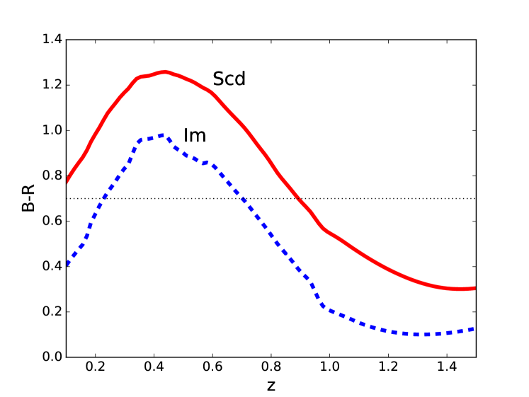
Figure 1: The $B-R$ color of a spiral (Scd) and irregular (Im) galaxy, highlighting the color-redshift degeneracies. The galaxy templates are from Benítez et al. (2004) and are normalized to have the same observed flux. We approximate the $B$ and $R$ filters as tophat filters centered at $4450~{}\AA$ and $6580~{}\AA$ with widths of $700~{}\AA$ and $1000~{}\AA$ respectively. An example color-redshift degeneracy is highlighted by the dotted line at $B-R=0.7$; this color is consistent with the irregular galaxy at $z\sim 0.2$ and $\sim 0.7$ and the spiral galaxy at $z\sim 0.9$.

We now imagine observing this population of galaxies with a low-resolution spectroscopic survey. We follow our example above, selecting galaxies with a fixed $B-R=0.7$ color and unit $R$-band flux. Fig. 2 plots the predicted spectrum for different admixtures of types and redshifts. For definiteness, we assume that the spiral galaxies form the dominant population, with the irregulars being contaminants. For this particular example, we find that the $\lambda>1\mu m$ part of the spectrum can determine the overall contamination fraction. The differences between contaminants at different redshifts (here $z\sim 0.2$ and $0.7$) are smaller, although with enough S/N, one can clearly start to distinguish these cases. The details are clearly specific to the case we have chosen here, but this demonstrates that an averaged spectrum can break degeneracies in photometric redshift distributions.

Furthermore, this figure allows us to schematically understand the depth requirements for the spectroscopic survey - given two degenerate (in $\cal P$) populations of galaxies, one needs to be able to distinguish between the stacked spectra in ${\cal S}$. As a numerical example, we suppose that stacking $10^{4}$ LSST galaxies in ${\cal S}$ yields a 10% detection of flux per frequency element and that ${\cal S}$ has $\sim 25-100$ frequency elements. Then we should be able to detect 1-2% differences in (total) flux in the spectrum, and distinguish between the different spectra in Fig. 2. The LSST gold sample ($i<25$) is expected to contain $\sim 4\times 10^{9}$ galaxies, which suggests that one could conceptually break the sample into $\sim 10^{5}$ voxels in magnitude space, each with sufficient galaxies to stack in the spectroscopic survey. The above estimates are just meant to be illustrative and to demonstrate that such an approach is feasible in principle.

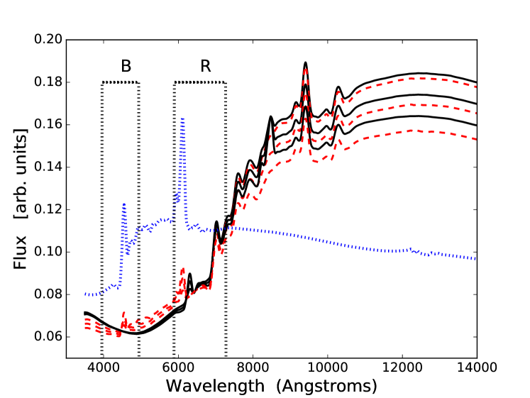
Figure 2: A demonstration that a stacked spectrum can be used to break degeneracies in photometric redshifts. From top to bottom, the lines show the expected stacked spectrum of spiral (Scd) galaxies with 10%, 20% and 30% contamination from a population of irregular (Im) galaxies. In all cases, the spiral galaxies are at a redshift of $\sim$0.9; the solid (black) lines have the irregular galaxies at $z\sim 0.7$, while the dashed (red) lines have the irregular galaxies at $z\sim 0.2$. By construction, all of these galaxies have the same $B-R$ color, and the same $R$-band magnitude. Also plotted for reference [dotted] is the irregular galaxy spectrum at $z=0.2$ (with an arbitrary vertical shift for clarity), and the nominal $B$ and $R$ bands we use.

2.2 Example 2 : Fitting redshift distributions

The previous section demonstrated how the stacked spectrum could break degeneracies in photometric redshifts. We extend this idea to measuring the redshift distribution here. As in the previous section, we consider a mixture of spiral and irregular galaxies using the same templates used previously. The assumed redshift distributions are shown in Fig. 3. The forms we chose reflect the color-redshift degeneracies seen in Fig. 1; in particular, note the “contamination” of low-redshift spirals and irregulars. We imagine these galaxies are selected to have the same $R$-band flux, they have perfectly measured $B-R$ colors, and that this selection yields $10^{6}$ galaxies.

We now combine the above redshift distributions (for spirals and irregulars) into a single $B-R$ color distribution. We then split the sample into $\Delta(B-R)=0.1$ color bins from $B-R=0$ to $1.3$. For each of these color bins, we compute the stacked spectrum of all the galaxies in the bin. Fig. 1 shows that, in general, these stacked spectra are the combination of spiral and irregular galaxies at two different redshifts. We assume that stacking $10^{4}$ galaxies yields a 10% measurement of flux per frequency element in the spectroscopic survey, and we scale this error by $\sqrt{10^{4}/N}$ where $N$ is the number of galaxies in the $B-R$ bin under consideration. We also assume that the stacked spectrum is measured from $5000\AA$ to $14000\AA$ with $R\sim 100$, which yields $\sim 70$ frequency elements. The inputs to our algorithm are the $B-R$ color distribution and the stacked spectrum in each $\Delta(B-R)$ color bin. As with template-based photo-$z$ codes, we assume we have a complete set of spectral templates (in this case, the templates for spiral and irregular galaxies).

We parametrize the redshift distributions of each individual population (spiral or irregular) by step-wise constant distributions in $z$ with 100 bins from $z=0$ to $z=1.5$. Given a bin in $B-R$, Fig. 1 shows that only a small fraction of these redshift bins will have a consistent $B-R$ color. These redshift bins are the input variables to a least-squares fit to the observed (stacked) spectrum using Eq. 3. We impose additional constraints that $(dN/dz)_{\alpha,b}\geq 0$ and that $\sum_{z}(dN/dz)_{\alpha,b}=1$, where $b$ indexes the color bin, and the latter constraint normalizes the redshift distribution. After computing these redshift distributions over the individual color bins, we combine these using

$$\left(\frac{dN}{dz}\right)_{\alpha}=\sum_{b}N_{b}\left(\frac{dN}{dz}\right)_{\alpha,b}\,,$$ (4)

where $N_{b}$ is the number of galaxies in the $b^{\rm th}$ color bin.

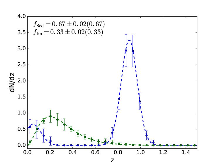
Figure 3: A test showing the recovered redshift distribution using stacked spectra. The dashed lines are the input redshift distributions for spiral (blue) and irregular (green) redshifts. The points show the recovered redshift distributions (averaged over 50 simulations), while the errorbars show the uncertainty expected for a single realization. Also shown are the fractions of spiral and irregular galaxies with the input values in parentheses. See the text for more details on the exact simulations.

Fig. 3 shows the redshift distribution recovered using the above procedure, averaging over the results of 50 simulations. Although we estimate the redshift distribution over 100 bins, the values between adjacent bins are highly covariant (since the spectra do not have the S/N to distinguish between small changes in redshift). We therefore average neighbouring bins to produce the figure shown. We also compress our results to the fractions of spiral and irregular galaxies, to mimic the case where the shape of the redshift distributions might be known (or well-constrained). We see that this simple procedure recovers the correct fractions of spiral and irregular galaxies as well as their redshift distributions. While this is a toy example, it illuminates the utility of these stacked spectra.

3 Discussion

We introduce the idea of “ensemble” photometric redshifts as a tool to constrain photometric redshift distributions. The idea is a simple extension of current template-based photometric redshift codes, and uses the fact that the shape of a stacked spectrum encodes information about the redshift distribution of the galaxies being stacked. The advantage of this approach is that the individual galaxies no longer need to be detected in the second survey, opening up the possibilities of using planned low-resolution shallower spectroscopy surveys like J-PAS, PAU and SPHEREx to calibrate deeper surveys like DES and LSST. An important point is that the next generation of imaging surveys will have samples of $\sim 10^{9}$ galaxies, which allows one to build large numbers of subsamples, each of which have sufficient numbers of galaxies to stack in the shallower survey. We outline the idea in this paper, and discuss some simple examples demonstrating how these stacked spectra can be used to break photometric redshift degeneracies and measure redshift distributions. These examples are meant to be illustrative; future work will be needed to understand the signal to noise for realistic galaxy distributions for future surveys.

An aspect of the ensemble photo-$z$ method is that one simultaneously fits both the individual photometric redshifts and the redshift distribution. We outline a simplified algorithm here, where we imagine splitting the original sample into voxels in magnitude space. This problem has also recently been considered by Leistedt, Mortlock & Peiris (2016) who discuss a more general approach to this problem; their algorithm can be easily extended to include constraints from the stacked spectrum. We expect that future work will also consider optimal algorithms for the next generations of surveys.

Our approach here has been to stack sources to get a detection in the shallower survey. Clearly, if one has well characterized errors, it is clear that the same information can be recovered by fitting observed fluxes (even if they are individual non-detections). We were however motivated by the fact that stacking the galaxies allows us to develop better intuition for the process. It also opens up possibilities for detecting mismatches in photometric redshift templates used, which could be folded back into photometric redshift codes. It should be emphasized that this entire process requires that one can average down the noise in the shallow spectroscopic survey, which will impose requirements on the data reduction and calibration.

Although the examples presented here used simple models for galaxy populations, our formalism is straightforward to extend to more complex cases. One such complication is the effect of dust, which will smear a single population at a fixed redshift along a line of extinction. We can imagine introducing parameters describing the scatter in extinction/reddening as well as its direction into our model, and then simultaneously fitting/marginalizing these with the redshift distributions. We defer a detailed study of this and other real-world complications to future work.

The problem of determining the photometric redshifts for the next generation of surveys is still an open question. It has been long recognized that increasing the wavelength coverage can improve photometric redshifts; however, it is normally assumed that these additional data should be matched in depth to the primary survey. We point out that, for the specific problem of determining the redshift distribution, this is not necessary, opening up the possibility for alternative/easier routes to calibrating photometric redshift distributions.

NP is supported in part by DOE DE-SC0008080. T.-C. C. acknowledges support from MoST grant 103-2112-M- 001-002-MY3 and the Simons Foundation. This work was begun and completed at the Aspen Center for Physics, which is supported by National Science Foundation grant PHY-1066293. This work made extensive use of the NASA Astrophysics Data System and of the astro-ph preprint archive at arXiv.org. Part of the research described in this paper was carried out at the Jet Propulsion Laboratory, California Institute of Technology, under a contract with the National Aeronautics and Space Administration.

References

- Benítez (2000) Benítez N., 2000, ApJ, 536, 571
- Benitez et al. (2014) Benitez N. et al., 2014, ArXiv e-prints
- Benítez et al. (2004) Benítez N. et al., 2004, ApJ Suppl., 150, 1
- Benjamin et al. (2010) Benjamin J., van Waerbeke L., Ménard B., Kilbinger M., 2010, MNRAS, 408, 1168
- Benjamin et al. (2013) Benjamin J., et al., 2013, MNRAS, 431, 1547
- Castander et al. (2012) Castander F. J. et al., 2012, in Proc. SPIE, Vol. 8446, Ground-based and Airborne Instrumentation for Astronomy IV, p. 84466D
- Choi et al. (2016) Choi A. et al., 2016, MNRAS, 463, 3737
- Dahlen et al. (2013) Dahlen T. et al., 2013, ApJ, 775, 93
- Doré et al. (2014) Doré O. et al., 2014, ArXiv e-prints
- Erben et al. (2009) Erben T. et al., 2009, A&A, 493, 1197
- Hildebrandt et al. (2010) Hildebrandt H. et al., 2010, A&A, 523, A31
- Ho et al. (2008) Ho S., Hirata C., Padmanabhan N., Seljak U., Bahcall N., 2008, Phys. Rev. D, 78, 043519
- Hoekstra & Jain (2008) Hoekstra H., Jain B., 2008, Annual Review of Nuclear and Particle Science, 58, 99
- Leistedt, Mortlock & Peiris (2016) Leistedt B., Mortlock D. J., Peiris H. V., 2016, ArXiv e-prints
- Limber (1953) Limber D. N., 1953, ApJ, 117, 134
- Limber (1954) Limber D. N., 1954, ApJ, 119, 655
- LSST Science Collaboration et al. (2009) LSST Science Collaboration et al., 2009, ArXiv:0912.0201
- Matthews & Newman (2010) Matthews D. J., Newman J. A., 2010, ApJ, 721, 456
- Matthews et al. (2013) Matthews D. J., Newman J. A., Coil A. L., Cooper M. C., Gwyn S. D. J., 2013, ApJ Suppl., 204, 21
- Matute et al. (2012) Matute I. et al., 2012, A&A, 542, A20
- McQuinn & White (2013) McQuinn M., White M., 2013, MNRAS, 433, 2857
- Ménard et al. (2013) Ménard B., Scranton R., Schmidt S., Morrison C., Jeong D., Budavari T., Rahman M., 2013, ArXiv e-prints
- Moles et al. (2008) Moles M. et al., 2008, AJ, 136, 1325
- Molino et al. (2014) Molino A. et al., 2014, MNRAS, 441, 2891
- Newman (2008) Newman J. A., 2008, ApJ, 684, 88
- Newman et al. (2015) Newman J. A. et al., 2015, Astroparticle Physics, 63, 81
- Padmanabhan et al. (2007) Padmanabhan N., et al., 2007, MNRAS, 378, 852
- Phillipps (1985) Phillipps S., 1985, MNRAS, 212, 657
- Phillipps & Shanks (1987) Phillipps S., Shanks T., 1987, MNRAS, 227, 115
- Rahman et al. (2015) Rahman M., Ménard B., Scranton R., Schmidt S. J., Morrison C. B., 2015, MNRAS, 447, 3500
- Rau et al. (2015) Rau M. M., Seitz S., Brimioulle F., Frank E., Friedrich O., Gruen D., Hoyle B., 2015, MNRAS, 452, 3710
- Sánchez et al. (2014) Sánchez C. et al., 2014, MNRAS, 445, 1482
- Schmidt et al. (2013) Schmidt S. J., Ménard B., Scranton R., Morrison C., McBride C. K., 2013, MNRAS
- Schulz (2010) Schulz A. E., 2010, ApJ, 724, 1305
- Seldner & Peebles (1979) Seldner M., Peebles P. J. E., 1979, ApJ, 227, 30