Using matrix product states to study the dynamical large deviations of kinetically constrained models

Abstract

Here we demonstrate that tensor network techniques — originally devised for the analysis of quantum many-body problems — are well suited for the detailed study of rare event statistics in kinetically constrained models (KCMs). As concrete examples we consider the Fredrickson-Andersen and East models, two paradigmatic KCMs relevant to the modelling of glasses. We show how variational matrix product states allow to numerically approximate — systematically and with high accuracy — the leading eigenstates of the tilted dynamical generators which encode the large deviation statistics of the dynamics. Via this approach we can study system sizes beyond what is possible with other methods, allowing us to characterise in detail the finite size scaling of the trajectory-space phase transition of these models, the behaviour of spectral gaps, and the spatial structure and “entanglement” properties of dynamical phases. We discuss the broader implications of our results.

Introduction.– Dynamics equipped with local kinetic constraints provides a general mechanism for slow cooperative relaxation Palmer et al. (1984); Fredrickson and Andersen (1984); Jäckle and Eisinger (1991); Kob and Andersen (1993). Kinetically constrained models (KCMs) — of which the Fredrickson-Andersen (FA) Fredrickson and Andersen (1984) and East Jäckle and Eisinger (1991) facilitated spin models are the simplest exponents — give many insights into the nature of glass forming systems, in particular by showing that systems with simple thermodynamics can have rich, spatially fluctuating and slow dynamics Garrahan and Chandler (2002). (For reviews on the glass transition see Binder and Kob (2011); Berthier and Biroli (2011); Biroli and Garrahan (2013), and on KCMs see Ritort and Sollich (2003); Garrahan et al. (2011); Garrahan (2018).) Beyond glasses, classical KCMs (and related deterministic models Prosen and Mejía-Monasterio (2016); Inoue and Takesue (2018); Prosen and Buča (2017); Klobas et al. (2018); Buča et al. (2019)) are relevant to the problem of operator spreading in quantum systems Nahum et al. (2017); Rowlands and Lamacraft (2018); Chen and Zhou (2018); Gopalakrishnan (2018); Knap (2018); Tran et al. (2018); Gopalakrishnan et al. (2018); Alba et al. (2019) and to non-equilibrium dynamics of ensembles of Rydberg atoms Lesanovsky and Garrahan (2013); Urvoy et al. (2015); Valado et al. (2016), while quantum KCMs provide a template for complex non-equilibrium dynamics under unitary evolution in the absence of disorder van Horssen et al. (2015); Smith et al. (2017); Lan et al. (2018); Turner et al. (2018).

To characterise dynamics it is natural to study ensembles of stochastic trajectories, just like one does in equilibrium statistical mechanics with ensembles of configurations. For long-times one can then apply the methods of dynamical large deviations (LDs) Touchette (2009) to compute quantities that play the role of thermodynamic potentials for the dynamics. For the case of KCMs this “thermodynamics of trajectories” approach reveals the existence of a first-order phase transition in the space of trajectories between active and inactive dynamical phases, indicative of the singular change when fluctuating away from typical behaviour Garrahan et al. (2007, 2009). Many other systems have been also shown to have similar LD transitions, see e.g. Lecomte et al. (2007); Appert-Rolland et al. (2008); Hedges et al. (2009); Speck et al. (2012); Weber et al. (2013); Espigares et al. (2013); Jack et al. (2015); Karevski and Schütz (2017); Baek et al. (2017); Oakes et al. (2018). Understanding the phase structure of the dynamics is clearly as important in dynamical problems as it is in static ones.

The standard way of accessing LD statistics of a dynamical observable is by computing its scaled cumulant generating function (SCGF) — see below for definitions — from the largest eigenvalue of an appropriate deformation, or tilting, of the generator of the dynamics Touchette (2009); Garrahan (2018). Except for the handful of non-trivial cases in which it can be calculated exactly Appert-Rolland et al. (2008); Buča et al. (2019), obtaining the SCGF by diagonalising the tilted generator is only possible for small system sizes. To access the LD behaviour for larger sizes one has to resort to numerical methods for sampling rare trajectories based on splitting/cloning, importance sampling or optimal control Giardina et al. (2006); Cérou and Guyader (2007); Lecomte and Tailleur (2007); Nemoto et al. (2016); Hedges et al. (2009); Ray et al. (2018); Klymko et al. (2018); Ferré and Touchette (2018).

By exploiting the similarity between tilted generators and quantum Hamiltonians, here we show how to use variational matrix product states (MPS) to compute numerically with high accuracy (and precise control on errors) leading eigenvalues and eigenstates of the tilted generator for system sizes way beyond those accessible through other methods. We study in detail the FA and East models, focusing on the finite size scaling of their active-inactive phase transitions and the spatial structure that emerges in the dynamical phases. While in certain special cases MPS can be used to obtain exact LD statistics, such as in simple exclusion processes Derrida and Lebowitz (1998); de Gier and Essler (2011); Lazarescu and Mallick (2011); Gorissen et al. (2012); Crampé et al. (2016), hard core brownian particles Lapolla and Godec (2018), and certain cellular automata Buča et al. (2019), the systematic application of numerical MPS methods to stochastic lattice systems has been limited Gorissen et al. (2009). Our results for KCMs — together with the very recent ones Helms et al. (2019) for simple exclusion processes — show the potential of numerical tensor network methods for the detailed study of dynamical fluctuations in stochastic dynamics.

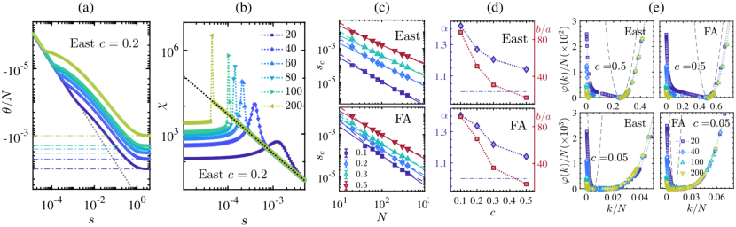
Figure 1: Finite size scaling of trajectory transition. (a) SCGF $\theta(s)/N$ as a function of $s$ for the East model ($c=0.2$) for system sizes $N=20$ to $N=200$. The critical $s_{c}(N)$ can be obtained from the (extrapolated) crossing of the first two energy levels. The dot-dashed lines correspond to the asymptotic values $\theta(s\to\infty)=-c$. (b) The corresponding dynamical susceptibilities, $\chi(s)=\theta^{\prime\prime}(s)$, exhibit a peak at $s_{c}(N)$ that gets narrower and higher as $N$ increases. For $s>s_{c}(N)$ we find an almost universal behavior $\chi\propto s^{-\gamma}$ with $\gamma\approx 1.4$. (c) $s_{c}(N)$ as a function of $N$ for $N\in[20,400]$ and various equilibrium concentrations $c$ in the East model (top) and FA model (bottom). As expected the data is compatible with $\lim_{N\to\infty}s_{c}(N)\to 0$, but $s_{c}$ appears to scale as $s_{c}(N)\propto N^{-\alpha}$ with $\alpha>1$ (full lines are power-law fits; for comparison we also show fits to $a/N+b/N^{2}$, dashed). (d) The scaling exponents $\alpha$ (blue diamonds) and fitting parameters $b/a$ (red squares) as a function of $c$ (top, East model; bottom, FA model). The departure from $1/N$ scaling (dotted-dashed) appears to be more pronounced the lower the $c$ is. (e) Rate functions $\varphi(k)$ for $N\in[20,200]$ for the East model (left) and FA model (right) at $c=0.5$ (top) and $c=0.05$ (bottom). The dashed lines correspond to Poisson distributions with average $\langle k\rangle=-\theta^{\prime}(0)/N$.

FA and East models.– The FA Fredrickson and Andersen (1984) and East Jäckle and Eisinger (1991) models are defined in terms of binary variables, $\{n_{i}=0,1\}_{i=1}^{N}$, on the sites of a one dimensional lattice of size $N$, with single-spin flip dynamics subject to a kinetic constraint such that a spin can flip up (with rate $c$) or down (with rate $1-c$) only if either nearest neighbour is in the up state (FA model) or only if the leftmost nearest neighbour is in the up state (East model). The generators for the corresponding continuous time Markov chains are Ritort and Sollich (2003); Garrahan et al. (2011); Garrahan (2018)

$$W^{\rm FA} =\sum_{i}\left(n_{i-1}+n_{i+1}\right)\left[c\sigma_{i}^{+}+(1-c)\sigma_{i}^{-}\right.$$

$$\left.-c(1-n_{i})-(1-c)n_{i}\right],$$ (1)

$$W^{\rm East} =\sum_{i}n_{i-1}\left[c\sigma_{i}^{+}+(1-c)\sigma_{i}^{-}\right.$$

$$\left.-c(1-n_{i})-(1-c)n_{i}\right],$$ (2)

where $\sigma_{i}^{\pm}$ flips the site $i$ up/down, and the factor in front of the square brackets is the kinetic constraint. In this formulation the master equation is $\partial_{t}|P\rangle=W|P\rangle$, where $|P\rangle$ is the probability vector over configurations.

We consider open boundary conditions which formally corresponds to setting $n_{0}=n_{N+1}=0$ in Eqs. (1) and (2). This is the best setup for the MPS method we use below. Due to the kinetic constraints configuration space can be disconnected, and we consider the dynamics within the largest ergodic component: the set of all configurations with at least one up site for the FA model, and all the configurations with fixed $n_{1}=1$ for the East model.

The dynamics has as stationary distribution $|P_{\rm eq}\rangle$ given by a projection of the product state $|c\rangle^{\otimes N}$, where $|c\rangle=(1-c)|0\rangle+c|1\rangle$, into the relevant ergodic component, giving

$$|P_{\rm eq}^{\rm FA}\rangle =[|c\rangle^{\otimes N}-(1-c)^{N}|0\rangle^{\otimes N}]/[1-(1-c)^{N}],$$ (3)

$$|P_{\rm eq}^{\rm East}\rangle =|1\rangle\otimes|c\rangle^{\otimes N-1}.$$ (4)

These are the equilibrium distributions with energy $E=\sum_{i}n_{i}$ at inverse temperature $\ln(1-c)/c$ in the corresponding ergodic components.

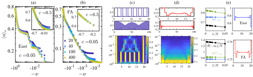
Figure 2: Structure of active phase. (a) Mean density $\langle n\rangle_{s}$ in the active phase, $s<0$, in the East model for the case $c=0.05$ (shown as function of $-\nu=e^{s}-1$). For small $c$ the plateau structure of the density is evident (as compared to $c=0.5$ in the inset). (b) Same for the FA model, where the plateaus are absent. (c) Density profile of the ground state of $H_{s}$ at $\nu=0.081$ ($s=-0.0845$) for the East model at $c=0.05$ for sizes $N=20,100$ (top and middle panels) and density profiles across the active phase for $N=20$ (bottom panel). (d) Same for the FA model at $c=0.05$. For the East model the state has pronounced anticorrelations which are absent in the FA case model. (e) Extreme limit of the active phase, $s\to-\infty$, for the East and FA models (top and bottom, respectively). In the panels on the right the symbols show the rescaled $\tilde{\theta}(s=-\infty)/N:=e^{s}\theta(s=-\infty)/[N\sqrt{c(1-c)}]$ (black circles), $\langle n\rangle_{s=-\infty}$ (blue squares) and $\langle n^{x}\rangle_{s=-\infty}$ (green diamonds) for $N\in[20,400]$. The lines are fits to $a/N+b$ to extract the values in the thermodynamic limit: $\lim_{N\to\infty}\theta(s=-\infty)/N,\langle n^{x}\rangle_{s=-\infty},\langle n\rangle_{s=-\infty}=0.67,0.82,0.75$ (East) and $1.34,0.82,0.75$ (FA). The right panels show (for $N=20$) that the density profiles at $s=-\infty$ are uniform, up to boundaries, in both models.

Dynamical LDs and tilted generators.– As trajectory observable we will consider the dynamical activity Lecomte et al. (2007); Garrahan et al. (2007); Baiesi et al. (2009), given by the total number of configuration changes $K(\omega_{t})$ (i.e., number of spin flips) in a trajectory $\omega_{t}$ of time extent $t$. For large $t$ the distribution of $K$ obeys a LD principle, $P_{t}(K)=\langle\delta[K(\omega_{t})-K]\rangle\approx e^{-t\varphi(K/t)}$, where $\varphi(x)$ is the LD rate function Touchette (2009). The corresponding moment generating function $Z_{T}(s)=\langle e^{-sK(\omega_{t})}\rangle$ also obeys a LD principle, $Z_{T}(s)\approx e^{t\theta(s)}$, where $\theta(s)$ is the scaled cumulant generating function (SCGF), whose derivatives at $s=0$ give the cumulants of $K$ (scaled by $t$) Touchette (2009). The LD functions are connected by a Legendre transform, $\theta(s)=-\min_{k}\left[sk+\varphi(k)\right]$ Touchette (2009) and play the role of thermodynamic potentials for trajectories.

The SCGF can be obtained from the largest eigenvalue of a tilted generator, $W_{s}$ Touchette (2009). For the case of the dynamical activity, the tilt corresponds to multiplying the off-diagonal terms of $W$ by a factor $e^{-s}$ Garrahan et al. (2007); Lecomte et al. (2007). Since the dynamics obeys detailed balance, the generators can be made hermitian by a similarity transformation which is independent of $s$ Garrahan et al. (2009). That is, if we define $H_{s}=-Q^{-1}W_{s}Q$, where $Q$ is a diagonal matrix with elements $\langle{\bf n}|Q|{\bf n}\rangle=(1-c)^{N/2}[c/(1-c)]^{\sum_{i}n_{i}/2}$ in the configuration basis $\{|{\bf n}\rangle\}$, we get

$$H^{\rm FA}_{s} =-\sum_{i}\left(n_{i-1}+n_{i+1}\right)$$ (5)

$$\times\left[e^{-s}\sqrt{c(1-c)}\sigma_{i}^{x}-c(1-n_{i})-(1-c)n_{i}\right],$$

$$H^{\rm East}_{s} =-\sum_{i}n_{i-1}\left[e^{-s}\sqrt{c(1-c)}\sigma_{i}^{x}\right.$$ (6)

$$\left.\phantom{\sqrt{c(1-c)}}-c(1-n_{i})-(1-c)n_{i}\right],$$

The SCGF therefore corresponds to (minus) the ground state energy of $H_{s}$,

$$\theta(s)=-E_{\rm GS}(s).$$ (7)

The relation between the ground state $|{\Phi_{s0}}\rangle$ of the tilted Hamiltonian, $H_{s}|{\Phi_{s0}}\rangle=E_{\rm GS}(s)|{\Phi_{s0}}\rangle$, and the left $\langle L_{s}|$ and right $|R_{s}\rangle$ leading eigenvectors of the tilted generator, $W_{s}|R_{s}\rangle=\theta(s)|R_{s}\rangle$, $\langle L_{s}|W_{s}=\langle L_{s}|\theta(s)$, is

$$|{\Phi_{s0}}\rangle=\sum_{\bf n}\sqrt{l_{\bf n}(s)r_{\bf n}(s)}\,|{\bf n}\rangle$$ (8)

where $l_{\bf n}(s)=\langle L_{s}|{\bf n}\rangle$ and $r_{\bf n}(s)=\langle{\bf n}|R_{s}\rangle$. The aim now is to compute $E_{\rm GS}(s)$ and $|{\Phi_{s0}}\rangle$ for Eqs. (5) and (6).

Variational MPS method.– For a lattice of $N$ $d$-dimensional quantum systems, a MPS Perez-Garcia et al. (2007) is a vector $|\Psi\rangle=\sum_{i_{1},\ldots i_{N}=1}^{d}\mathrm{tr}\left(A_{1}^{i_{1}}A_{2}^{i_{2}}\ldots A_{N}^{i_{N}}\right)|i_{1}i_{2}\ldots i_{N}\rangle$, where $i_{k}$ labels a local basis of the $k-$th subsystem, and each $A_{k}$ is a rank-$3$ tensor of dimensions $d\times D\times D$ . Such a state is described by $O(dND^{2})$ parameters. The bond dimension $D$ limits the entanglement of the state. More precisely, in an MPS of bond dimension $D$, for any subchain $A$ the entanglement entropy (defined as $S_{\rm E}=-{\rm Tr}_{A}\rho_{A}\log\rho_{A}$, where $\rho_{A}={\rm Tr}_{N\setminus A}|\Psi\rangle\langle\Psi|$ Nielsen and Chuang (2011)) is upper-bounded by $S_{\rm E}\leq 2\log D$, independent of the subchain length. Namely, MPS satisfy an entanglement area law Eisert et al. (2010), and conform a hierarchy of increasingly entangled states, with $D=d^{N/2}$ sufficing to describe the whole Hilbert space.

Conversely, MPS can efficiently approximate states that satisfy an area law , such as ground states of gapped local Hamiltonians. They thus are the basis for numerical methods like the celebrated density matrix renormalization group (DMRG) algorithm White (1992) which can be understood as a variational minimization of energy over MPS Vidal (2003); Verstraete et al. (2004); McCulloch (2007); Verstraete et al. (2008); Schollwöck (2011), by sequientially optimizing a single tensor, while keeping the rest constant, and iteratively sweeping over the chain until convergence . Formulated in terms of tensor networks this algorithm allows a number of extensions, including simulating dynamics, and the calculation of a few excited states above the ground state.

We apply this strategy to find MPS approximations to the ground state and first excitations of the Hamiltonians (5) and (6). In this case, $d=2$ and the basis is $\{|{\bf n}\rangle\}$. As we show below, MPS with $D\ll 2^{N}$ provide accurate approximations for systems sizes at an order of magnitude larger than those accessible by other methods .

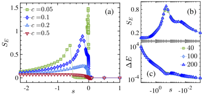
Figure 3: Entanglement. (a) Half-chain entanglement entropy $S_{E}$ of the ground state of $H_{s}$ as a function of $s$ for $c=0.5,0.1,0.05$ in the East model at $N=200$. (b) $S_{E}$ for $s<0$ for $c=0.1$ at various sizes $N$. The peak is correlated with the change in shape of the spectral gap $\Delta E$ of $H_{s}$ shown in (c).

Results. Finite size scaling of active-inactive trajectory transition.– The key property of KCMs like the FA and East is their first-order phase transition between an active phase for $s<0$ and inactive dynamical phase at $s>0$ Garrahan et al. (2007, 2009), manifested in a first-order singularity in the SCGF in the limit of $N\to\infty$. Like for all phase transitions, to characterise the transition and its associated fluctuations, it is necessary to understand how the singularity is approached as the system size increases. Theoretical and numerical considerations Bodineau et al. (2012); Bodineau and Toninelli (2012); Nemoto et al. (2017) suggest that for finite $N$ the (rounded) transition occurs at $s_{c}(N)>0$ (i.e. typical dynamics, $s=0$, is perturbatively connected to the active phase), and $s_{c}(N)\to 0^{+}$ as $1/N$. These predictions can be tested with our MPS method.

Figure 1(a) shows (minus) the energy density $-E_{\rm GS}(s)/N=\theta(s)/N$ of the MPS solution as a function of $s$. The transition at $s_{c}(N)$ occurs where the two branches cross. The leftmost branch is linear in $s$ and proportional to $N$, corresponding to the linear response for $s\gtrsim 0$ (grey dashed line). The rightmost branch is nonlinear, connecting the regime at $s\gtrsim 0$ to the asymptotic $\theta(\infty)=-c$. The corresponding susceptibility $\chi_{s}=\theta^{\prime\prime}(s)/N$ shows a diverging peak at $s_{c}(N)$, see Fig. 1(b) Note (4).

We can estimate the location of $s_{c}(N)$ from the susceptibility peak. For both models we find a departure from the expected $1/N$ scaling. Figure 1(c) shows that $s_{c}(N)$ can be fit to a power law, $s_{c}(N)\propto N^{-\alpha}$ with $\alpha>1$ throughout. An alternative is that this discrepancy is due to subleading corrections to $1/N$, see Fig. 1(c) (dashed lines), and Fig. 1(d) for the dependence of the scaling parameters with $c$. We also show in Fig. 1(e) the broadening with $N$ of the LD rate function, indicative of the first order transition Garrahan et al. (2007, 2009). For more details on the finite size scaling analysis including comparison with the predictions of the Ref. Bodineau et al. (2012) see SM .

Structure of active phase.– While both models have similar active-inactive transitions, their active phases differ. Figures 2(a,b) show the average density of excitations, $\langle n\rangle_{s}=N^{-1}\sum_{i=1}^{N}\langle{\Phi_{s0}}|n_{i}|{\Phi_{s0}}\rangle$, in the MPS that approximates the ground state of $H_{s}$ for $s<0$. In the East model and for small $c$, $\langle n\rangle_{s}$ shows a series of plateaus as $s$ becomes more negative, as predicted in Ref. Jack and Sollich (2013). These plateaus are absent in the FA model at the same $c$, Fig. 2(b), and also when the equilibrium concentration $c$ is high, see insets to Figs. 2(a,b).

Figures 2(c,d) show the difference in spatial structure of the active phases. The top two panels in Fig. 2(c,d) give the density profile at $s=-0.0845$ ($\nu=0.081$) corresponding to the plateau in Fig. 2(a) with density $\langle n\rangle_{s}\approx 1/3$. For the East model, Fig. 2(c, top two panels), the state is anticorrelated in space, with an occupied site followed by two nearly empty ones. This is evident in the $N=20$ case, shown in the figure, while for $N=100$ we also observe a longer ranged modulation of this pattern Note (4). In contrast, in the FA model the density is essentially uniform, Fig. 2(d, top two panels). This difference in structure is present throughout the $s<0$ phase, see bottom panels of Fig. 2(c,d).

We can also characterise the extreme active limit $s\to-\infty$. We find that a MPS of $D\sim O(10)$ is enough to obtain a very precise approximation to the ground state over the whole range of sizes computed, $N\in[20,\,400]$. We can then extrapolate to $N\to\infty$. We obtain, Fig. 2(e), for the limiting SCGFs $\lim_{N\to\infty}\lim_{s\to-\infty}e^{s}\theta_{\mathrm{E}}(s)/[N\sqrt{c(1-c)}]\approx 0.6687$ for the East and $1.337$ for the FA model, while the densities are the same in both models, namely $\lim_{N\to\infty}\langle n\rangle_{-\infty}\approx 0.754$ and $\lim_{N\to\infty}\langle n^{x}\rangle_{-\infty}\approx 0.824$ (where $n^{x}$ is up to constants the “transverse” magnetisation, $2n^{x}=1-N^{-1}\sum_{i=1}^{N}\sigma_{i}^{x}$). The panels on the right of Fig. 2(e) show that the corresponding density profiles are essentially flat in this limit .

Entanglement.– The states at $s\neq 0$ have spatial correlations absent in equilibrium ($s=0$) and which varies with $s$. This can be quantified via their entanglement entropy, which together with other quantum information measures can capture changes in dynamical behaviour that might escape classical order parameters Castelnovo et al. (2010). The entanglement entropy is easily computed for a state in MPS form. Figure 3(a) shows the half-chain $S_{E}$ of the state $|{\Phi_{s0}}\rangle$ as a function of $s$ in the East model at size $N=200$. It is zero in the equilibrium state, cf. Eq. (4), and very small in the inactive phase, where the leading eigenvector is close to a product state of all sites empty in the bulk. For $s<0$ it shows interesting structure, as expected from the spatial correlations of Fig. 2. In Fig. 3(b) we notice that the maximum of $S_{\rm E}$ does not seem to scale with system size. Thus, in the language of quantum many-body systems, the ground state fulfils an area law. This is also the case for other entropic quantities Note (4), which justifies the accuracy of the MPS approximation.

The peak in $S_{E}$ nevertheless is sensitive to changes in the structure of the active phase. Fig. 3(c) shows the corresponding gap between $E_{\rm GS}(s)$ and the eigenvalue of the first excited state: its $s$ dependence changes at a value of $s$ located by the peak in $S_{E}$. (Note also that the gap is has no significant $N$ dependence.) The maximum of the entropy depends on the value of $c$, and we find a larger peak for smaller values, corresponding to richer structure in the active phase, see Fig. 3(a) and Note (4).

Even if the entanglement is low throughout the phase diagram, cf. Fig. 3(a), this does not guarantee that the variational method will easily find an MPS approximation. In fact, we find that both for the region close to the phase transition at $s=0$ and for the values of $s$ where $S_{\rm E}$ shows a peak, cf. Fig. 3(a,b), the numerical convergence is slower than would have been expected. We believe this is a consequence of how the spectrum of the Hamiltonian changes when approaching these regimes Note (4).

Conclusions.– As we have shown here, the MPS methods often employed in quantum many-body problems Schollwöck (2011), are also well suited for the study of the dynamical generators of classical stochastic systems Derrida and Lebowitz (1998); de Gier and Essler (2011); Lazarescu and Mallick (2011); Gorissen et al. (2012); Crampé et al. (2016); Lapolla and Godec (2018); Buča et al. (2019); Gorissen et al. (2009); Prosen and Mejía-Monasterio (2016); Inoue and Takesue (2018); Prosen and Buča (2017); Klobas et al. (2018); Helms et al. (2019). We focused on the LD statistics of KCMs such as the FA and East models, and showed how variational MPS approximations allow to efficiently access system sizes which are larger by an order of magnitude compared to previous studies, thus providing detailed information about the properties of the transitions in these models and the nature of the dynamical phases. We foresee many other applications of tensor networks in classical stochastic dynamics, including when the dynamical transition is continuous rather than first-order, and in the study of systems in dimension larger than one. More broadly, the crossover of ideas and techniques between quantum many-body and classical stochastics remains a fruitful area of investigation.

Acknowledgements – This work was supported by the Deutsche Forschungsgemeinschaft (DFG, German Research Foundation) under Germany’s Excellence Strategy – EXC-2111 – 390814868, by EPSRC Grant No. EP/R04421X/1 and by the Leverhulme Trust Grant No. RPG-2018-181. We acknowledge the hospitality of the Kavli Institute for Theoretical Physics at the University of California, Santa Barbara, where this work was started, and support from the National Science Foundation under Grant No. NSF PHY-1748958.

I Supplemental Material

II Numerical method

The main MPS algorithm employed for this work is the variational optimization of a MPS with open boundary conditions, in order to solve the minimization

$$|\Psi\rangle=\mathrm{argmin}\frac{\langle\Psi|H|\Psi\rangle}{\langle\Psi|\Psi\rangle},$$ (S1)

over the set of MPS with fixed bond dimension $D$. The solution is the MPS approximation to the ground state of the Hamiltonian $H$. There are many reviews in the literature describing the development, technical details and applications of tensor network algorithms like this one, as well as their extensions to infinite systems, finite temperature and dynamics, and possible extensions to higher dimensions  Schollwöck (2011); Verstraete et al. (2008).

It is convenient to express the algorithm fully in terms of tensor networks, by writing the Hamiltonian as a matrix product operator (MPO) McCulloch (2007); Pirvu et al. (2010), i.e. a MPS vector in the tensor product basis of operators (that is, as a linear combination of products of Pauli matrices). Local Hamiltonians as the ones considered in this work have an exact MPO expression with small constant bond dimension $D_{H}$ that does not depend on the system size. Evaluating its expectation value in a MPS of bond dimension $D$, which is the fundamental ingredient for the variational minimization of the energy, has then a cost that scales as $O(dD_{H}D^{3})$ in terms of the tensor dimensions, and linearly with the system size. This is crucial for the efficiency of the variational algorithm. In particular, we can write the East Hamiltonian model for open boundary conditions with bond dimension $D_{H}=3$ (or 4 for periodic chains) and the FA Hamiltonian with $D_{H}=4$ (or 6 for periodic boundary conditions).

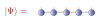
(a) Pictorial representation of a MPS.

(b) A local Hamiltonian has an exact MPO form.

(c) The norm as contraction of the state with its adjoint over the physical indices.

(d) The energy is computed as the expectation value of an MPO in a MPS state.

(e) The effective norm at one site $\mathcal{N}_{\mathrm{eff}}$ is obtained leaving out from the norm the tensors corresponding to the site.

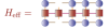
(f) Effective Hamiltonian $\mathcal{H}_{\mathrm{eff}}$ as a TN.

Figure S1: Tensor networks and their contractions can be represented in a convenient pictorial language, which simplifies the description of algorithms and operations. A solid geometrical form (e.g. circles or squares above) represents a tensor, with as many indices as depicted legs. A contraction of two tensors over a certain index is represented as a connecting line. The pictures show the graphical representation of MPS, MPO and their contractions, as they appear in the variational algorithm.

The variational optimization then proceeds by fixing all tensors of the ansatz

$$|\Psi\rangle=\sum_{i_{1},\ldots i_{N}=1}^{d}\mathrm{tr}\left(A_{1}^{i_{1}}A_{2}^{i_{2}}\ldots A_{N}^{i_{N}}\right)|i_{1}i_{2}\ldots i_{N}\rangle$$ (S2)

but the one for site $k$, $A_{k}$, and rewriting the optimization (S1) as a local problem in terms of the single variable tensor. The local problem boils down to a generalized eigenvalue problem for the vectorized tensor, $\mathcal{H}_{\mathrm{eff}}A_{k}=\lambda_{\min}\mathcal{N}_{\mathrm{eff}}A_{k}$  Schollwöck (2011); Verstraete et al. (2008), where $\mathcal{H}_{\mathrm{eff}}$ ($\mathcal{N}_{\mathrm{eff}}$) is an effective Hamiltonian (norm matrix) of dimension $dD^{2}\times dD^{2}$, obtained by contracting all tensors in $\langle\Psi|H|\Psi\rangle$ and in $\langle\Psi|\Psi\rangle$, except for $A_{k}$; see a pictorial representation in Fig. S1. This problem can then be solved with a standard eigensolver from a linear algebra numerical package, and the minimum eigenvalue $\lambda_{\min}$ corresponds to the estimate of the ground state energy. Using a sparse eigensolver allows to keep the cost scaling as $D^{3}$ and to deal with very large values of the bond dimension. The $k$-th tensor is updated with the solution of the local optimization, and then the procedure is repeated for all the tensors in the chain, sweeping back and forth until a certain convergence criterion (typically on the energy) is met. The same algorithm can be used to find higher excited states by imposing that the solution is orthogonal to already found levels. This can be imposed at the level of the local problem, without changing the scaling of the leading cost, which is always $\mathcal{O}(D^{3})$ (and grows polynomially with the number of computed levels).

For a run with fixed bond dimension, the algorithm is guaranteed to converge, because it can only decrease the energy in every step, although it may do so to a local minimum. To improve the precision, one increases the bond dimension of the ansatz, typically using the previous solution with smaller $D$ as initial guess. In a typical application, the algorithm is repeatedly run with increasing bond dimension, until the energy of the state is converged to the desired precision . A notorious case in which the algorithm is slow to converge is that of critical systems, where the ground state requires a bond dimension that grows polynomially with the system size in order to achieve a fixed precision, a situation that is well understood by DMRG practitioners. But on the other hand, having a state that can be well approximated by a MPS does not guarantee convergence of the algorithm. A large density of states also hinders convergence, as happens for instance when trying to approximate excited states in the middle of the spectrum.

II.1 Convergence

(a) East $s=-10^{-5}$

(b) East $s=3\cdot 10^{-6}$

(c) FA $s=-10^{-5}$

(d) FA $s=3\cdot 10^{-6}$

Figure S2: Convergence of the energy as a function of the bond dimension in some of the most difficult cases ($c=0.05$ and small values of $s$).

(a) $c=0.5$ $s<0$

(b) $c=0.5$ $s>0$

(c) $c=0.05$ $s<0$

(d) $c=0.05$ $s>0$

Figure S3: Energy standard deviation (square root of variance) $\Delta H=\sqrt{\langle H^{2}\rangle-\langle H\rangle^{2}}$ in the MPS approximation to the ground state for the East model. The plots show, for system sizes $N=20$ (blue) and $400$ (red) the systematic lowering of the variance as the bond dimension is varied from $D=2$ (squares), to $10$ (diamonds) and $20$ (triangles). We show the detail of the most difficult regions, namely the region of the plateaus for small $s<0$ (S3a and S3c) and the region of small $s>0$ around the phase transition (S3b and S3d). By letting the algorithm run longer until a maximum bond dimension $D=100$, the variance of the peaks is reduced to $\Delta H\lesssim 10^{-5}$.

(a) $c=0.5$ $s<0$ $D=20$

(b) $c=0.5$ $s>0$ $D=20$

(c) $c=0.05$ $s<0$ $D=20$

(d) $c=0.05$ $s>0$ $D=20$

Figure S4: Energy standard deviation (square root of variance) $\Delta H=\sqrt{\langle H^{2}\rangle-\langle H\rangle^{2}}$ in the MPS approximation to the ground state for the FA model. Qualitatively, we observe similar effects as for the East model, described in figure S3, As in figure S3, we show the systematic lowering of the variance as the bond dimension is varied from $D=2$ (squares), to $10$ (diamonds) and $20$ (triangles) for system sizes $N=20$ (blue) and $400$ (red). Again, bond dimension $D<100$ is enough to ensure very small variance over the most challenging range of parameters.

We find the ground states over the largest part of the parameter space to be very well approximated by MPS with small bond dimension. The quality of the MPS approximation can be gauged from the convergence of observables as the bond dimension is increased. We find this to be in general very fast, even for system sizes of several hundred sites. We let the algorithm use bond dimensions as large as $D=100$, but in most of the cases analyzed, we find that a bond dimension $D=20$ is enough for the energy to be sufficiently converged. As illustrated in figure S2, only in a few cases, mostly for small values of $c$ and around the phase transition, we find that a larger bond dimension allows us to reach a lower energy. We also find that convergence becomes difficult for large systems when we try to explore the region of the phase transition at small positive $s$ in both models. Since we have demonstrated that the states do not develop a large entropy, even in this region, we attribute this behaviour to the density of states at the lowest energy becoming larger for increasing system size.

A more accurate measure of how close the approximation is to an actual eigenstate is however provided by the energy variance, $\Delta H^{2}=\langle H^{2}\rangle-\langle H\rangle^{2}$, which can be computed efficiently for any MPS. In the cases studied in the paper, we find that a very small bond dimension, $D=20$, is already enough to obtain a very small variance $\Delta H^{2}\lesssim\mathcal{O}(10^{-10})$ for a wide range of values of $s$ and all system sizes up to $N=400$ (see the upper row of figures S3 and S4). The exceptions are the region of the phase transition at small $s>0$ in both models, specially as $c$ decreases (see figures S3b, S3d, S4b and S4b).

III Detailed numerical results

III.1 Finite size scaling of the active-inactive phase transition

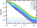
(a) (Minus) energy density as a function of $s$

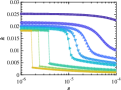
(b) Activity as a function of $s$

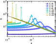
(c) Susceptibility as a function of $s$

Figure S5: Scaling of the phase transition location for the East model with $c=0.1$.

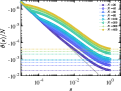
(a) (Minus) energy density as a function of $s$

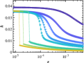
(b) Activity as a function of $s$

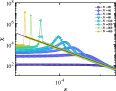
(c) Susceptibility as a function of $s$

Figure S6: Scaling of the phase transition location for the FA model with $c=0.1$.

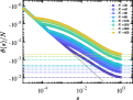
(a) (Minus) energy density as a function of $s$

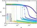
(b) Activity as a function of $s$

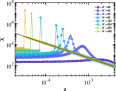
(c) Susceptibility as a function of $s$

Figure S7: Scaling of the phase transition location for the FA model with $c=0.2$.

To study the finite size scaling of the active-inactive phase transition we have simulated both models for varying system sizes $N\in[20,400]$ over a range of values for the equilibrium concentration $c\in[0.05,0.5]$. We observe that all cases conform qualitatively to the behaviour discussed in the main text, and explicitly shown for the East model at $c=0.2$ [Fig. 1(a,b) in the main text]. The (normalized) SCGF, shown in Figs. S5a, S6a and S7a, which equals minus the energy density of the ground state, varies linearly with $s$, in agreement with the perturbative calculation around $s=0$. The grey dashed line in the figures shows the linear response prediction in the thermodynamic limit, namely $\theta/N=-2c^{2}(1-c)s$ for the East and $\theta/N=-4c^{2}(1-c)s$ for the FA model. The intersection of this line with the asymptotic value for $s\to\infty$, shown as dashed coloured lines in the plots, scales as $1/N$. However, in the figures it is evident that the value of $s_{c}$ at which the actual crossing occurs can be orders of magnitude away from this prediction.

The activity

$$k=-\frac{\theta^{\prime}(s)}{N}=\frac{1}{N}\frac{dE_{\rm GS}(s)}{ds}$$ (S3)

can also be directly evaluated from the MPS ansatz, since

$$\frac{dE_{\mathrm{GS}}}{ds}=\langle\Psi|\frac{dH}{ds}|\Psi\rangle,$$ (S4)

only requires computing the expectation value of local and two-body observables. The results are shown in figures  S5b, S6b and S7b. The numerical derivative of the activity yields the susceptibility $\chi=\frac{d\theta^{2}}{ds^{2}}$, shown in Figs. S5c, S6c and S7c. The location $s_{c}$ of the phase transition for each system size is most precisely determined from the position of the peak in $\chi$.

An alternative FSS analysis of the transition can be made by following the approach of Bodineau, Lecomte and Toninelli in Ref. Bodineau and Toninelli (2012) (hereafter BLT) which considers in detail the FA model. BLT use the fact that within a region of size $1/N$ around the transition, that is for $s$ of order $1/N$ or equivalently for $\lambda=sN$ with $\lambda=O(1)$, the SCGF in terms of $\lambda$, $\phi(\lambda)=\theta(\lambda/N)$ is of $O(1)$ [rather than of $O(N)$ as for $s$ finite] and should progressively interpolate between two behaviours at large $N$ (see also Bodineau et al. (2012)). The two behaviours are that of linear response, $\phi=-\langle k\rangle\lambda$, for $\lambda<\lambda_{c}$, and a regime of constant $\phi=-\Sigma$ for $\lambda\geq\lambda_{c}$. Here $\Sigma$ is a “surface tension” related to the creation of an interface between the active and inactive phases, while $\langle k\rangle$ is the equilibrium activity per unit time. Figure S8 presents the SCGF in this representation for both models, cf. Fig. 2 of Ref. Bodineau and Toninelli (2012). The crossover between these two regimes is apparent both in the FA, as described by BLT, and also in the East model. Note that accessing the constant regime on the right is more difficult for lower $c$.

The prediction of BLT is that $\phi(\lambda)+\Sigma$ should behave as $-A\lambda^{\nu}$ for $\lambda>\lambda_{c}$. Figure S9 shows such a scaling for both the FA model and the East model, cf. Fig. 3 of Bodineau and Toninelli (2012). We have estimated the exponent $\nu$ and the constant $\Sigma$ in the following way. Since the activity is (minus) the first derivative of the SCGF, in the relevant region it should scale as $\lambda^{\nu-1}$ [cf. the scaling of the susceptibility in Fig. 1(b) of the main text]. This allows to obtain $\nu$ without the need to simultaneously fit $\Sigma$. As discussed above, the activity can be calculated efficiently as it corresponds to the contraction of an MPO with the MPS. Figure S10 shows the activity for both models. The smaller $c$ is the larger the system size $N$ is required to be to accurately extract $\nu$. With the exponent $\nu$ in hand we can then estimate $\Sigma$ by subtracting the $\lambda$ dependence from $\phi$. This is illustrated in Fig. S11c(a,b) for $c=0.5$ for both models.

For the FA model, BLT found $\Sigma\approx 0.077$ for the surface tension at $c=0.5$. In our case, for the FA model we find $\Sigma\approx 0.077/2$ at $c=0.5$, see Fig. S11c(a), the factor of a half coming from the fact that we use open boundary conditions (which allows a single interface to be created, in contrast to the periodic boundary condition case). This result seems to confirm the BLT prediction. For the East model we find a slightly lower value at $c=0.5$, $\Sigma\approx 0.032$, see Fig. S11c(b). As Fig. S11c(c) shows, we observe that $\Sigma$ decreases significantly with $c$, with $\Sigma$ seemingly going as $\Sigma\propto c^{\xi}$ with $\xi\approx 3.3$ for the FA model (and decreasing even faster with $c$ for the East model). For the exponent, BLT predicted $\nu=2/3$. While for large $c$ this is compatible with our findings, see Fig. S10, we seem to find that $\nu$ increases with decreasing $c$. Nevertheless, this discrepancy might be due to the fact that for smaller values of $c$ extracting both $\Sigma$ and $\nu$ gets progressively more difficult.

(a) FA $c=0.5$

(b) FA $c=0.1$

(c) East $c=0.5$

(d) East $c=0.1$

Figure S8: SCGF $\phi(\lambda)$ with $\lambda=sN$ in transition region, cf. Fig. 2 of Ref. Bodineau and Toninelli (2012), for various sizes. The dashed line is the linear response behaviour.

(a) FA $c=0.5$

(b) FA $c=0.3$

(c) FA $c=0.2$

(d) FA $c=0.05$

(e) East $c=0.5$

(f) East $c=0.3$

(g) East $c=0.2$

(h) East $c=0.05$

Figure S9: Collapse of SCGF $\phi(\lambda)$ for $\lambda>\lambda_{c}$, cf. Fig. 3 of Ref. Bodineau and Toninelli (2012).

(a) FA $c=0.5$

(b) FA $c=0.1$

(c) East $c=0.5$

(d) East $c=0.1$

Figure S10: Activity $k(s)$. From the region where the curves collapse we can extract the exponent $\nu$ used in Fig. S9. We only show two values of $c$ for comparison, but this procedure was used to extract $\nu$ for all other $c$.

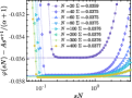
(a) FA $c=0.5$

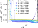
(b) East $c=0.5$

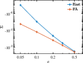
(c) East $c=0.5$

Figure S11: (a) SCGF after subtracting the term proportional to $\lambda^{\nu}$ in order to estimate $\Sigma$ for the FA model. (b) Same for East model. (c) Surface tension $\Sigma$ as a function of $c$ for both models extracted by the procedure of panels (b,c) for all available $c$. For the FA model we get $\Sigma\propto c^{\xi}$ with $\xi\approx 3.3(2)$.

III.2 Structure of active phase

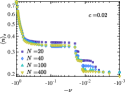
(a) East model, $c=0.02$

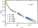
(b) East model, $c=0.1$

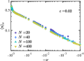
(c) FA model

Figure S12: Average occupation in the active phase as a function of $-\nu=e^{s}-1$. For the East model (two leftmost plots), plateaus appear for small values of the equilibrium concentration, up to $c=0.1$ (central plot), where we only observe a cusp at $\nu\sim 0.14$ ($s\sim-0.13$). For larger values of $c$, the curve is smooth (see the inset of Fig. 2(a) in the main text), the same as for the FA model over the whole range of values of $c$.

(a) $c=0.02$

(b) $c=0.05$

(c) $c=0.1$

(d) $c=0.5$

Figure S13: Spatial distribution of density $n_{i}=(1-\langle\sigma_{i}^{z}\rangle)/2$ in the active phase of the East model as a function of $s$ for a chain of length $N=20$ and increasing value of $c$.

(a) $c=0.02$

(b) $c=0.05$

(c) $c=0.1$

(d) $c=0.5$

Figure S14: Spatial distribution of density $n_{i}=(1-\langle\sigma_{i}^{z}\rangle)/2$ in the active phase of the FA model as a function of $s$ for a chain of length $N=20$ and increasing value of $c$.

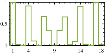
(a) $N=18$

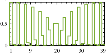
(b) $N=39$

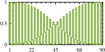
(c) $N=90$

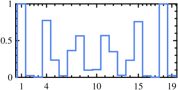
(d) $N=19$

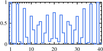
(e) $N=40$

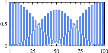
(f) $N=100$

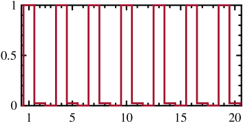
(g) $N=20$

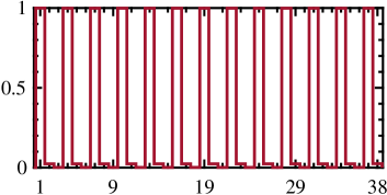
(h) $N=38$

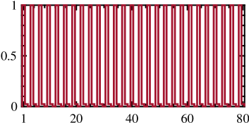
(i) $N=80$

Figure S15: Distribution of density along the chain for $c=0.02$ and $s=-0.1$ (in the middle of the $\langle n\rangle_{s}=1/3$ plateau in Fig. S13a) depending on the congruence of the chain length modulo $3$ being $0$ (left column), $1$ (center) or $2$ (right column).

As discussed in the main text, the active phase of both models exhibits very different features, which we can explore with our results. In the East model, for small values of $c$, we recover the hierarchy of plateaus with well defined average density predicted in Jack and Sollich (2013), extending between values of $\nu=1-e^{s}$ equal to integer powers of $c$. This is clearly appreciated in Fig. S12a for $c=0.02$, where the plateau at $\langle n\rangle=1/3$ which ends at $\nu=0.02$ is already converged in system size. For $c=0.1$ there is no plateau structure anymore, but a cusp remains in the average density at $\nu\sim 0.14$, as shown in Fig. S12b, while for yet larger values of $c$, the curve is smooth (see for instance the inset of figure 2(a) in the main text). For the FA model, on the other hand, there are no similar features in the average density, as shown explicitly by Fig. S12c and figure 2(b) in the main text.

To explore in more detail the structure of the active phase in both models, we have computed the spatial dependence of the density across the same range of values of $s$ spanned by Fig. S12. We show the results for a system size $N=20$ in figures S13 (for the East) and  S14 (for the FA model). In the case of the East model, the figure shows how the fixed average density of the plateaus is achieved by means of a regular modulation of the local density. For the $\langle n\rangle_{s}=1/3$ plateau, the state has one occupied site followed by two almost empty ones, a structure that the density plots in S13 clearly show. The extension of the plateau decreases, and the position of its boundary moves to larger $s$ as $c$ increases, and they have disappeared completely at $c=0.5$ (fig. S13d). For the FA model, on the other hand, no plateaus occur for any value of $c$, as explicitly shown by Fig. S14 for $c\in[0.02,0.5]$.

The period three modulation of density shown in Fig. S13 for the case of $N=20$ is present also in larger systems, but the detailed structure depends on the congruence modulo three of the system size. This is shown explicitly in Fig. S15, for the particular case $c=0.02$, $s=-0.1$ and different system sizes.

III.3 Entanglement

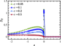
(a) $N=200$

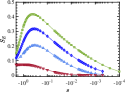
(b) Active phase of $N=200$

Figure S16: Entropy in the ground state of the FA model. The left plot shows the overall behaviour with respect to $s$ for a chain of size $N=200$ and different values of $c$, and the right one shows the detail of the active phase.

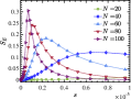
(a) East model $c=0.05$.

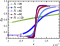
(b) FA model $c=0.05$.

Figure S17: Entropy around $s=0$ in the ground state of the East and FA model at $c=0.05$ for different system sizes.

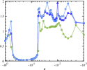
(a) $S_{\alpha}$, $\alpha=0.5$

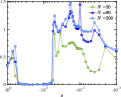
(b) $S_{\alpha\to 1}=S_{\rm E}$

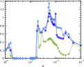
(c) $S_{\alpha}$, $\alpha=2$

Figure S18: Entanglement in the active phase of the East model, as measured by the von Neumann and Renyi entropies $S_{\alpha}$ of the half-chain for $c=0.05$ and various system sizes (congruent to 2 modulo 3).

The states we are looking for contain very little entanglement. We have shown explicitly in the main text that the entanglement entropy with respect to a division of the chain in two $S_{\rm E}$ remains bounded by a constant even in the region of the phase transition for the East model [see Fig. 3 in the main text]. The same is true in the case of the FA model, as shown in Fig. S16a for a chain of length $N=200$. As one can expect from the previous discussion, in this case, no peaks of the entropy occur within the active phase, and the entropy is smooth for all values of $c$; see zoom in Fig. S16b, to be compared to Fig. 3(b) in the main text. The maximum of the entropy occurs, instead, around the phase transition, for small positive values of $s$, but the magnitude of the peak shows only a mild dependence on the system size, similar to what we observed in the East model.

There are however differences between both models in the behaviour of the entropy at very small $s$, as shown in Fig. S17. In the East model, the entropy at $s=0$ is strictly zero, corresponding to a product ground state [see Eq. (4) of the main text and Fig. S17a], and builds up to a peak around the transition. In the case of the FA model, the ground state at $s=0$, in the subspace orthogonal to the state with no excitations, is not a product state [see Eq. (3) of the main text], and thus the entropy is not exactly zero, but has a finite value at $s=0$, namely

$$S_{\rm E}^{\mathrm{FA}}(s=0)=\mathrm{H}\left(\frac{1}{2}\left[1+\sqrt{1-\left(\frac{2}{1+(1-c)^{-N/2}}\right)^{2}}\right]\right),$$ (S5)

where $\mathrm{H}(x)=-x\log_{2}x-(1-x)\log_{2}(1-x)$ is the Shannon entropy. The value of $S_{\rm E}^{\mathrm{FA}}(s=0)$ decreases fast with the system size $N$ (Fig. S17b). For $s>0$, $S_{\rm E}$ grows also in the case of the FA model, towards a value of order one. Afterwards we find an almost vanishing energy. Notice that to the right of the transition, in the limit $s\to\infty$, the ground state is doubly degenerate, and the component that is symmetric under parity, thus in the same subspace as the ground state at $s=0$, would have entanglement $S_{\rm E}=1$. However, at sufficiently large $s$, the algorithm prefers to break the symmetry to find a solution with smaller bond dimension.

The bounded entropy alone is not enough to guarantee the approximability of the ground state by a MPS Schuch et al. (2008). To gather more compelling evidence we can also study the scaling of Renyi entropies, defined as $S_{\alpha}=\mathrm{Tr}\rho^{\alpha}/(1-\alpha)$ for $\alpha>0$, and which in the limit $\alpha\to 1$ converge to the von Neumann entropy. An area law for a $S_{\alpha}$ with $\alpha<1$ would imply approximability of the state as a MPS, as demonstrated in Schuch et al. (2008). The MPS ansatz gives natural access to the Schmidt values for any cut of the chain, so that all $S_{\alpha}$ can be computed efficiently. We show the values of the von Neumann and Renyi entropies for the active phase of the East model with $c=0.05$ in the region of the plateaus (since it is the region with the largest entropy we found), in Fig. S18. Again we see that, although the magnitude of the peaks is not fully converged, the dependence on the system size is very mild.

References

- Palmer et al. (1984) R. G. Palmer, D. L. Stein, E. Abrahams, and P. W. Anderson, Phys. Rev. Lett. 53, 958 (1984).
- Fredrickson and Andersen (1984) G. H. Fredrickson and H. C. Andersen, Phys. Rev. Lett. 53, 1244 (1984).
- Jäckle and Eisinger (1991) J. Jäckle and S. Eisinger, Z. fur Phys. B 84, 115 (1991).
- Kob and Andersen (1993) W. Kob and H. C. Andersen, Phys. Rev. E 48, 4364 (1993).
- Garrahan and Chandler (2002) J. P. Garrahan and D. Chandler, Phys. Rev. Lett. 89 (2002).
- Binder and Kob (2011) K. Binder and W. Kob, Glassy materials and disordered solids: An introduction to their statistical mechanics (World Scientific, 2011).
- Berthier and Biroli (2011) L. Berthier and G. Biroli, Rev. Mod. Phys. 83, 587 (2011).
- Biroli and Garrahan (2013) G. Biroli and J. P. Garrahan, J. Chem. Phys. 138, 12A301 (2013).
- Ritort and Sollich (2003) F. Ritort and P. Sollich, Adv. Phys. 52, 219 (2003).
- Garrahan et al. (2011) J. P. Garrahan, P. Sollich, and C. Toninelli, in Dynamical Heterogeneities in Glasses, Colloids, and Granular Media, International Series of Monographs on Physics, edited by L. Berthier, G. Biroli, J.-P. Bouchaud, L. Cipelletti, and W. van Saarloos (Oxford University Press, Oxford, UK, 2011).
- Garrahan (2018) J. P. Garrahan, Physica A 504, 130 (2018).
- Prosen and Mejía-Monasterio (2016) T. Prosen and C. Mejía-Monasterio, J. Phys. A 49, 185003 (2016).
- Inoue and Takesue (2018) A. Inoue and S. Takesue, J. Phys. A 51, 425001 (2018).
- Prosen and Buča (2017) T. Prosen and B. Buča, J. Phys. A 50, 395002 (2017).
- Klobas et al. (2018) K. Klobas, M. Medenjak, T. Prosen, and M. Vanicat, arXiv:1807.05000 (2018).
- Buča et al. (2019) B. Buča, J. P. Garrahan, T. Prosen, and M. Vanicat, arXiv:1901.00845 (2019).
- Nahum et al. (2017) A. Nahum, J. Ruhman, S. Vijay, and J. Haah, Phys. Rev. X 7, 031016 (2017).
- Rowlands and Lamacraft (2018) D. A. Rowlands and A. Lamacraft, Phys. Rev. B 98, 195125 (2018).
- Chen and Zhou (2018) X. Chen and T. Zhou, arXiv:1808.09812 (2018).
- Gopalakrishnan (2018) S. Gopalakrishnan, Phys. Rev. B 98, 060302 (2018).
- Knap (2018) M. Knap, Phys. Rev. B 98, 184416 (2018).
- Tran et al. (2018) M. C. Tran, A. Y. Guo, Y. Su, J. R. Garrison, Z. Eldredge, M. Foss-Feig, A. M. Childs, and A. V. Gorshkov, arXiv:1808.05225 (2018).
- Gopalakrishnan et al. (2018) S. Gopalakrishnan, D. A. Huse, V. Khemani, and R. Vasseur, Phys. Rev. B 98, 220303 (2018).
- Alba et al. (2019) V. Alba, J. Dubail, and M. Medenjak, arXiv:1901.04521 (2019).
- Lesanovsky and Garrahan (2013) I. Lesanovsky and J. P. Garrahan, Phys. Rev. Lett. 111, 215305 (2013).
- Urvoy et al. (2015) A. Urvoy, F. Ripka, I. Lesanovsky, D. Booth, J. P. Shaffer, T. Pfau, and R. Löw, Phys. Rev. Lett. 114, 203002 (2015).
- Valado et al. (2016) M. M. Valado, C. Simonelli, M. D. Hoogerland, I. Lesanovsky, J. P. Garrahan, E. Arimondo, D. Ciampini, and O. Morsch, Phys. Rev. A 93, 040701 (2016).
- van Horssen et al. (2015) M. van Horssen, E. Levi, and J. P. Garrahan, Phys. Rev. B 92, 100305 (2015).
- Smith et al. (2017) A. Smith, J. Knolle, D. L. Kovrizhin, and R. Moessner, Phys. Rev. Lett. 118, 266601 (2017).
- Lan et al. (2018) Z. Lan, M. van Horssen, S. Powell, and J. P. Garrahan, Phys. Rev. Lett. 121, 040603 (2018).
- Turner et al. (2018) C. Turner, A. Michailidis, D. Abanin, M. Serbyn, and Z. Papić, Nature Phys. 14, 745 (2018).
- Touchette (2009) H. Touchette, Phys. Rep. 478, 1 (2009).
- Garrahan et al. (2007) J. P. Garrahan, R. L. Jack, V. Lecomte, E. Pitard, K. van Duijvendijk, and F. van Wijland, Phys. Rev. Lett. 98, 195702 (2007).
- Garrahan et al. (2009) J. P. Garrahan, R. L. Jack, V. Lecomte, E. Pitard, K. van Duijvendijk, and F. van Wijland, J. Phys. A 42, 075007 (2009).
- Lecomte et al. (2007) V. Lecomte, C. Appert-Rolland, and F. van Wijland, J. Stat. Phys. 127, 51 (2007).
- Appert-Rolland et al. (2008) C. Appert-Rolland, B. Derrida, V. Lecomte, and F. van Wijland, Phys. Rev. E 78, 021122 (2008).
- Hedges et al. (2009) L. O. Hedges, R. L. Jack, J. P. Garrahan, and D. Chandler, Science 323, 1309 (2009).
- Speck et al. (2012) T. Speck, A. Malins, and C. P. Royall, Phys. Rev. Lett. 109, 195703 (2012).
- Weber et al. (2013) J. K. Weber, R. L. Jack, and V. S. Pande, J. Am. Chem. Soc. 135, 5501 (2013).
- Espigares et al. (2013) C. P. Espigares, P. L. Garrido, and P. I. Hurtado, Phys. Rev. E 87, 032115 (2013).
- Jack et al. (2015) R. L. Jack, I. R. Thompson, and P. Sollich, Phys. Rev. Lett. 114, 060601 (2015).
- Karevski and Schütz (2017) D. Karevski and G. M. Schütz, Phys. Rev. Lett. 118, 030601 (2017).
- Baek et al. (2017) Y. Baek, Y. Kafri, and V. Lecomte, Phys. Rev. Lett. 118, 030604 (2017).
- Oakes et al. (2018) T. Oakes, S. Powell, C. Castelnovo, A. Lamacraft, and J. P. Garrahan, Phys. Rev. B 98, 064302 (2018).
- Giardina et al. (2006) C. Giardina, J. Kurchan, and L. Peliti, Phys. Rev. Lett. 96, 120603 (2006).
- Cérou and Guyader (2007) F. Cérou and A. Guyader, Stoch. Anal. Appl. 25, 417 (2007).
- Lecomte and Tailleur (2007) V. Lecomte and J. Tailleur, J. Stat. Mech. 2007, P03004 (2007).
- Nemoto et al. (2016) T. Nemoto, F. Bouchet, R. L. Jack, and V. Lecomte, Phys. Rev. E 93, 062123 (2016).
- Ray et al. (2018) U. Ray, G. K.-L. Chan, and D. T. Limmer, J. Chem. Phys. 148, 124120 (2018).
- Klymko et al. (2018) K. Klymko, P. L. Geissler, J. P. Garrahan, and S. Whitelam, Phys. Rev. E 97, 032123 (2018).
- Ferré and Touchette (2018) G. Ferré and H. Touchette, J. Stat. Phys. 172, 1525 (2018).
- Derrida and Lebowitz (1998) B. Derrida and J. L. Lebowitz, Phys. Rev. Lett. 80, 209 (1998).
- de Gier and Essler (2011) J. de Gier and F. H. L. Essler, Phys. Rev. Lett. 107, 010602 (2011).
- Lazarescu and Mallick (2011) A. Lazarescu and K. Mallick, Journal of Physics A: Mathematical and Theoretical 44, 315001 (2011).
- Gorissen et al. (2012) M. Gorissen, A. Lazarescu, K. Mallick, and C. Vanderzande, Phys. Rev. Lett. 109, 170601 (2012).
- Crampé et al. (2016) N. Crampé, E. Ragoucy, V. Rittenberg, and M. Vanicat, Phys. Rev. E 94, 032102 (2016).
- Lapolla and Godec (2018) A. Lapolla and A. Godec, New J. Phys. 20, 113021 (2018).
- Gorissen et al. (2009) M. Gorissen, J. Hooyberghs, and C. Vanderzande, Phys. Rev. E 79, 020101 (2009).
- Helms et al. (2019) P. Helms, U. Ray, and G. K.-L. Chan, arxiv:1904.07336 (2019).
- Baiesi et al. (2009) M. Baiesi, C. Maes, and B. Wynants, Phys. Rev. Lett. 103, 010602 (2009).
- Perez-Garcia et al. (2007) D. Perez-Garcia, F. Verstraete, M. M. Wolf, and J. I. Cirac, Quantum Inf. Comput. 7, 401 (2007).
- Note (1) In the case of open boundary conditions, as used in this work, the first and last tensors reduce to rank- tensors of dimensions .
- Nielsen and Chuang (2011) M. A. Nielsen and I. L. Chuang, Quantum Computation and Quantum Information: 10th Anniversary Edition, 10th ed. (Cambridge University Press, New York, NY, USA, 2011).
- Eisert et al. (2010) J. Eisert, M. Cramer, and M. B. Plenio, Rev. Mod. Phys. 82, 277 (2010).
- Note (2) Strictly speaking, the statement holds for states which fulfill an area law in Renyi entropies with Schuch et al. (2008).
- White (1992) S. R. White, Phys. Rev. Lett. 69, 2863 (1992).
- Vidal (2003) G. Vidal, Phys. Rev. Lett. 91, 147902 (2003).
- Verstraete et al. (2004) F. Verstraete, D. Porras, and J. I. Cirac, Phys. Rev. Lett. 93, 227205 (2004).
- McCulloch (2007) I. P. McCulloch, J. Stat. Mech. 2007, P10014 (2007).
- Verstraete et al. (2008) F. Verstraete, V. Murg, and J. Cirac, Adv. Phys. 57, 143 (2008).
- Schollwöck (2011) U. Schollwöck, Ann. Phys. 326, 96 (2011).
- Note (3) Notice that it is also possible to define MPS directly in the thermodynamic limit, and optimize them numerically with appropriate methods Verstraete et al. (2008); Schollwöck (2011).
- Note (4) For details on the MPS numerics, their convergence, and for the comprehensive set of results for both the FA and East models, see Supplemental Material.
- Bodineau et al. (2012) T. Bodineau, V. Lecomte, and C. Toninelli, J. Stat. Phys. 147, 1 (2012).
- Bodineau and Toninelli (2012) T. Bodineau and C. Toninelli, Commun. Math. Phys. 311, 357 (2012).
- Nemoto et al. (2017) T. Nemoto, R. L. Jack, and V. Lecomte, Phys. Rev. Lett. 118, 115702 (2017).
- (77) Supplemental Material.
- Jack and Sollich (2013) R. L. Jack and P. Sollich, J. Phys. A 47, 015003 (2013).
- Note (5) The GS in the limit seems to be gapped and with low entanglement ( provides a very good approximation Note (4)). The GS energy of the FA in this limit is almost exactly twice the one for East, and the overlap of their states is very high, suggesting they have similar GS, or rather the FA one is the superposition of that of the East and the reflected “West” model.
- Castelnovo et al. (2010) C. Castelnovo, C. Chamon, and D. Sherrington, Phys. Rev. B 81, 184303 (2010).
- Pirvu et al. (2010) B. Pirvu, V. Murg, J. I. Cirac, and F. Verstraete, New Journal of Physics 12, 025012 (2010), 0804.3976 .
- Note (6) See e.g. Schollwöck (2011) for more details on initialization, convergence criteria, etc.
- Schuch et al. (2008) N. Schuch, M. M. Wolf, F. Verstraete, and J. I. Cirac, Phys. Rev. Lett. 100, 030504 (2008).