Enhancing the efficiency of adiabatic quantum computations
Abstract
We describe a general methodology for enhancing the efficiency of adiabatic quantum computations (AQC). It consists of homotopically deforming the original “Hamiltonian surface” in a way that the redistribution of the Gaussian curvature weakens the effect of the anti-crossing, thus yielding the desired improvement. Our approach is not pertubative but instead is built on our previous global description of AQC in the language of Morse theory. Through the homotopy deformation we witness the birth and death of critical points whilst, in parallel, the Gauss-Bonnet theorem reshuffles the curvature around the changing set of critical points. Therefore, by creating enough critical points around the anti-crossing, the total curvature–which was initially centered at the original anti-crossing–gets redistributed around the new neighbouring critical points, which weakens its severity and so improves the speedup of the AQC. We illustrate this on two examples taken from the literature.
Key words: anti-crossing, critical points, homotopy, Morse theory, Cerf theory, Gauss-Bonnet theorem, quantum phase transition, non-stoquastic Hamiltonians.
1 Introduction
An important early result in quantum mechanics is the so-called avoided crossing, also anti-crossing theorem. It dates back to the work of J. von Neumann, and E. Wigner [14] – more accurately, two years earlier, to the work of F. Hund [9]; J. von Neumann and E. Wigner proved and generalized the intuition of F. Hund. Their finding is as follows (see also [12, 6]):
Suppose the Hermitian matrix depends on a number of parameters . Then when one can change only one or two parameters it is in general not possible to reach an intersection of the eigenvalues of . This number goes to one if is a real Hermitian matrix; that is, in this case it suffices to be able to change two real parameters to make two eigenvalues degenerate.
The role of anti-crossings in adiabatic quantum computations is well known [8, 13]. This is expressed as the total adiabatic evolution time being inversely proportional to the square of the energy difference between the two lowest energies of the given Hamiltonian
| (1) |
for . This energy gap, for many instances444By an instance, we mean a time dependent Hamiltonian; thus, we include the choice of the initial Hamiltonian in our definition–and not just the problem Hamiltonian., is very small, and the enlargement of this gap is the focal point in current research in the area of adiabatic quantum computations. The goal of our paper is to present a general principled methodology to study anti-crossings that generalizes previous studies (that are ad-hoc) and also provides guidelines for new constructions.
1.1 Connection to Morse functions
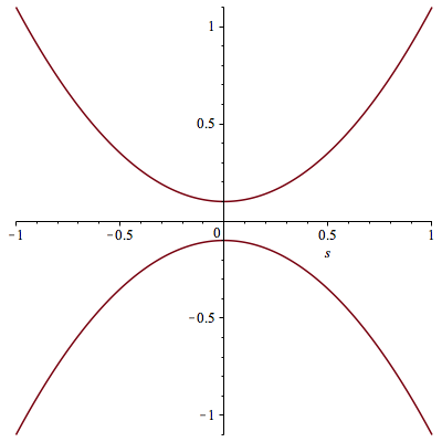
Let us start by making the connection with Morse theory [3]. Suppose and are two parallel planar curves; i.e., their tangent vectors span a two dimensional vector space (e.g., two eigenvalues of the time dependent Hamiltonian ). Let us assume that and are twice differentiable on a compact interval and satisfying for all in . Suppose at some point , the two curves converge to each other (without intersecting) and then diverge again; that is, is convex on while is concave. Without loss of generality, we can write
| (2) |
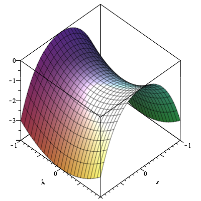
with . The spectral gap is minimized at the anti-crossing ; see Figure 1. Now, we embed the two planar curves into the three dimensional Euclidean space and define the function
The graph of the function is the saddle surface (also depicted in Figure 1). With this embedding, the anti-crossing point is mapped into a non degenerate critical point of with a negative Gaussian curvature 555Because , a point in is a non degenerate critical point of the function if and only if the remainder is not zero at , where is a Groebner basis for the ideal generated by the two polynomials and .. As we shall show, this embedding also constrains what can be done to the picture on the right in order to eliminate the anti-crossings and provides guidelines to how it can be done. The key constructions are gradient flows [1], the Euler characteristic, and the Gauss-Bonnet theorem [5] which distributes the curvature consistently with the Euler characteristic.
1.2 Outline of the paper
In section 2, we describe the general methodology for changing the dynamics around anti-crossing. We start by reviewing the connection with Morse theory and add more details than the simple connection we made in the Introduction. We then explain that the central object of our investigation is one (or more) parameter families of Hamiltonians and review the appropriate mathematical machinery, i.e., Cerf theory. The third section discusses two concrete illustrations of the general theory; these two situations are taken from published literature. The first situation repels the ground state from the rest of the spectrum while the second situation weakens first order quantum phase transitions (QPT) into a higher order. The role of the Gauss-Bonnet theorem is elucidated. We conclude with some suggestions for future research.
2 The general theory
We briefly review the Morse theoretical depiction of the adiabatic evolution of the Hamiltonian (1) that we have introduced in [6]. We then extend this depiction to parametrized families of Hamiltonians. For Morse theorists, this extension is referred to as Cerf theory.
2.1 Morse theory
To the Hamiltonian (1), we assign the Morse function given by the characteristics polynomial (aka secular function)
| (3) |
where is the identity matrix. The surface , aka cobordism in the language of Morse theory, is defined by the (non degenerate) critical points of using handlebodies decomposition [6]. This interplay between and the topology (homology) of the cobordism is the apex of Morse theory, and can be expressed in more precise terms as follows: the trajectories of the gradient flow
| (6) |
triangulate and the homology of this complex is isomorphic to the “usual” singular homology of . One can then work on the cobordism to investigate , or vice versa. This paper is aligned with the former.
If we Taylor series around each of its critical points (and rotate axes to coincide with principal curvature directions), we get a simple local expression of :
Lemma 1 (Morse lemma - Revisited)
Given i.e., a non degenerate critical point of the smooth function . We have
| (7) |
with being the principal curvature of at .
The lemma, which we use repeatedly, gives the two energies around the critical point as solutions of the equation (7). In particular, the energy difference between the two is given by
| (8) |
(after translating to the origin–it is important to notice that translations, as well as rotations- above, are isometries, i.e., distance preserving transformations). This gives
| (9) |
The square root is always real-valued: if is a saddle, i.e., an anti-crossing, then and . If is a maximum then and . If is a minimum then and .
Remarkably, the different local descriptions of can be glued together. The fact that these local depictions can be glued together is the incarnation of the globality of Morse theory. In the language of functors, this can be presented as follows: Let denote the category of standard open sets of sorted by inclusion and denote the category of real-valued smooth functions sorted by restrictions.
Proposition 1
The functor , defined by the lemma for each open set, is a sheaf.
For readers familiar with this language, the proof is almost evident, particularly when we take into account that critical points are isolated.
2.2 Cerf theory
As mentioned before, the central object in this paper is not the mere Hamiltonian (1) but the one-parameter families of Hamiltonians
| (10) |
This gives rise to a one-parameter family of Morse functions and to the homotopy:
| (11) |
with and . An important implication of the homotopy (11) is that the Euler characteristic is given independently of by the Gauss-Bonnet formula:
| (12) |
Because the curvature is essentially dumped at the critical points, the above formula constrains the quantities , and, by (8), the energy differences, simultaneously. In fact, for each critical point , we have
| (13) |
while at the same time we also have
| (14) |
where the neighbourhoods are the graph of (given by the lemma). Equivalently, we are constrained (in our quest of enhancement) by the commutativity of the following diagrams:
where is the unique global section of the functor . In particular, as changes, the set of critical points changes but consistently with the invariant homology groups. This means that critical points might move around and new critical points might appear (born), or old ones disappear (death), by pairs of (saddle, minimum) or (saddle, maximum), which amounts to adding, or deleting, a cylinder (surface with ), thus not affecting the topology.
3 Two illustrative examples
We give two illustrations of the general methodology described above, i.e, homotopically altering the dynamics around the anti-crossing by adding critical points to its vicinity (through the process of birth/death of critical pairs). In the first example, we push away the first excited state from the ground state by adding degeneracy, whilst in the second, we change a first order quantum phase transition (QPT) into a second order by adding non-stoquasticity. The role of the Gauss-Bonnet theorem is also exhibited in both cases.
3.1 Enhancement by degeneracy: Repelling the excited state
This section revisits the work of Dixon [4].
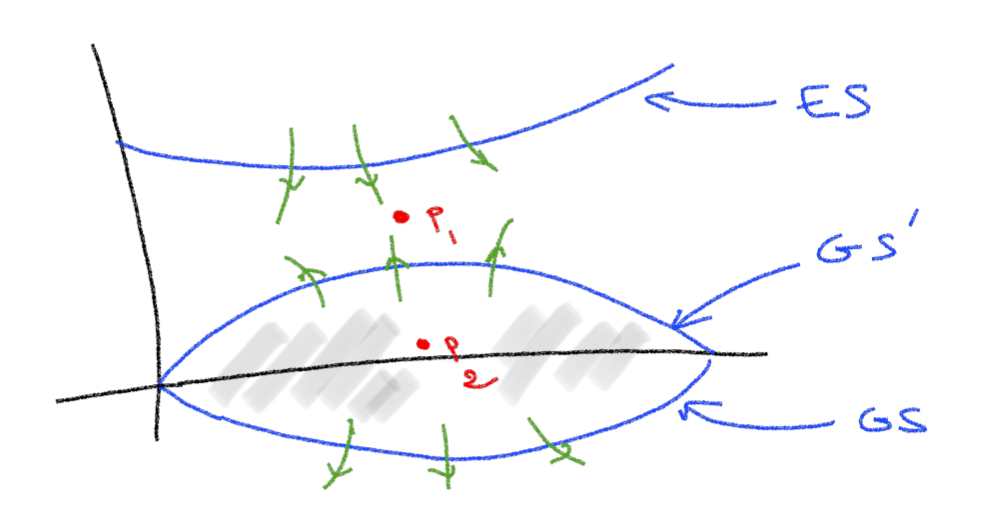
The main idea is described in Figure 2. Initially, the two lowest energies are attracted to each other due to the presence of an anti-crossing (as in (a)). The addition of a minimum (or maximum as depicted, by making the ground state degenerate at , will repel the rest of the spectrum from the ground state, simply because level sets around a minimum (or maximum) are ellipses ((b) and (c)). See also Figure 3.
To make this more concrete, consider the following situation where we initially have (Morse function of the Grover search adiabatic Hamiltonian [11, 6])
| (15) |
Similar to [4], we make the ground state degenerate at by defining the one parameter family of functions ():
| (16) |
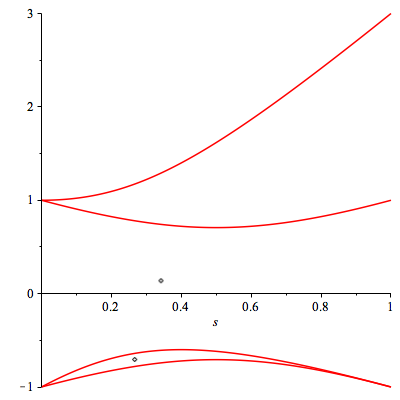
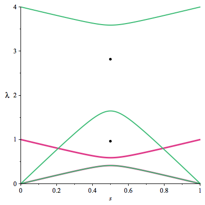
Here Let us, for instance, fix to 1 and to 5. The Morse function now has two critical points in the rectangular region where is a large number (see Figure 4):
| (17) |
Figures 4 and 5 also show that is a maximum while is an anti-crossing point (a saddle). When is infinitesimally small (it makes sense to take it infinitesimally small, because the addition of is affecting ony the direction; hence, we would like to concentrate on this direction), the two principal curvatures are essentially the same, i.e., (recall that the principal curvatures are by definition the maximum and minimum of the curvatures of all curves passing through the given point, and because the surface shrinks to a curve, the two are equal). The application of the Gauss Bonnet formula on the region , with being the surface depicted in (b) above, gives
| (18) |
which gives the functional dependence between and . Returning to our instance, a direct calculation of the two principal curvatures confirms this dependence:
3.2 From first order QPT to second order
When the system endures a first order QPT, the spectral gap between the two lowest energies is exponentially small, yielding exponentially large evolution time. The reason is quite simple. In a first order QPT, the two local minima that the ground state occupies before and after the transition are too far apart (in the Hamming distance sense), so the tunnelling is exponentially slow. This singularity is expressed mathematically by the discontinuity of the first derivative of the free energy. A higher order QPT comes with less severe shrinking of the spectral gap.
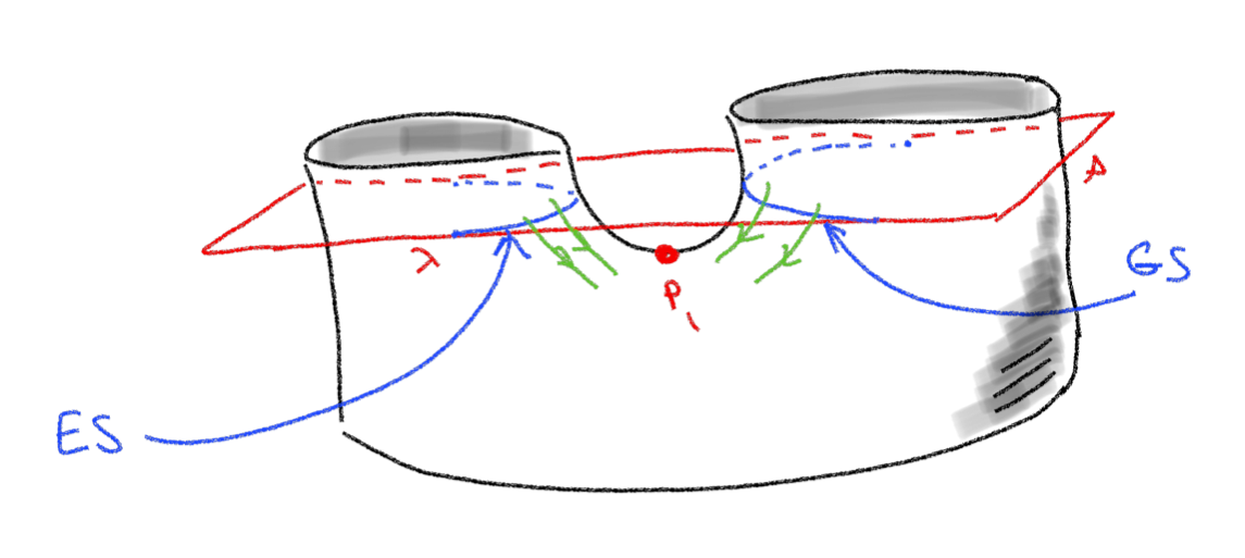
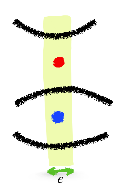
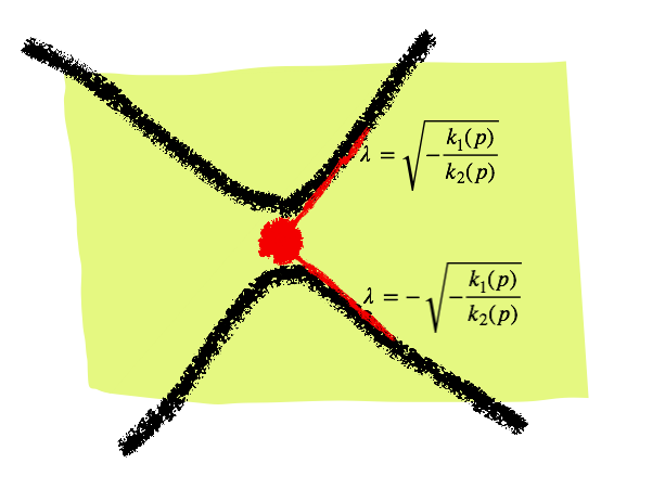
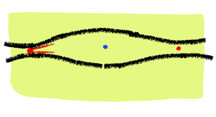
The bare bone idea of this section is depicted in the picture below. Initially, we have an anti-crossing in the region . The angle between the two asymptotes is given by
| (19) |
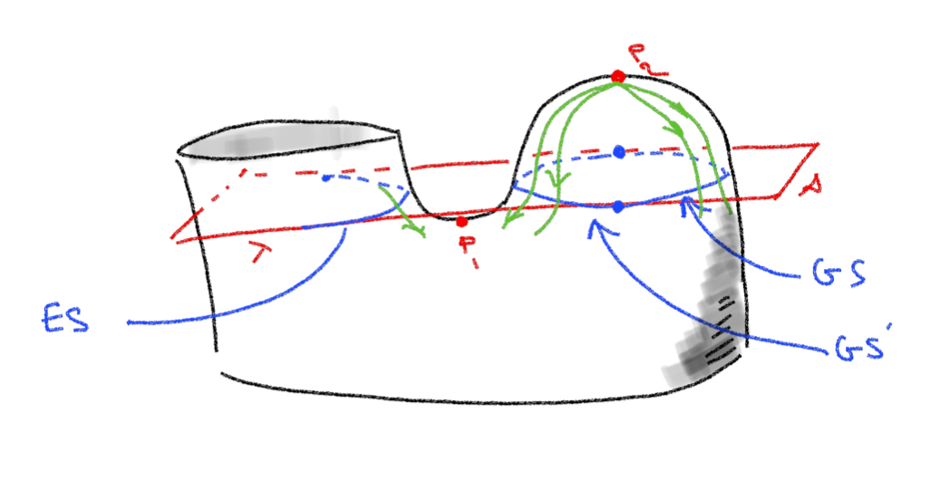
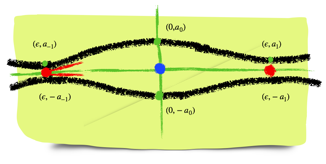
Here is the mean curvature. For first order QPTs, this angle is large, i.e., approaches . The figure on the right shows the birth of a pair (min, saddle) in the vicinity of the anti-crossing. The effect of this homotopical change is that the new angle is reduced. As before, the curvatures of the three critical points are related with the relation
Let us make this more concrete by considering the following, somewhat simplified, scenario:
The Morse function is given by
| (20) |
with
| (21) |
and for . Fix , with a large enough positive number– precisely, . Working out Gauss-Bonnet formula on yields the dependancy between the different curvatures:
| (22) | |||||
A better example would be to have two different parameters instead of just , so the distance between the minimum and the saddle is independent of their distance from the original saddle. The computation generalizes easily but gives complicated expressions.
3.2.1 The case of the ferromagnetic spin model
Here we pay a particular attention to the very instructive model of the ferromagnetic spin. See the work by Nishimori and Takada [10]. The time dependent Hamiltonian is given simply by
| (23) |
where the th power refers to the matrix power; i.e., composition of linear operators on the Hilbert space . A comprehensive investigation into the Hamiltonian can be found in [2]. This Hamiltonian exhibits a first order QPT for ; this can be shown in various ways–for instance, by taking the thermodynamical limit , in which case one gets a classical (continuous) spin of a single particle. Figure 8 shows the continuity and discontinuity of the first derivative of the classical energy when and respectively.
For finite , the system is also reduced into a much smaller space. This is because of the commutativity of with the total spin . Interestingly, this reduction can be generalized using the theory of irreducible representations [7], but here we recall the usual reduction. Conveniently, the lowest part of the spectrum of the total operator is also the lowest part of the spectrum of . And because of the anti-crossing theorem, this is also true for . This lowest part is given by the states with maximum spin i.e., states , for , and defined with
| (24) | |||||
| (25) |
In addition we have
| (26) |
where are the spin raising the lowering operators. All of this continues to hold with the new non-stoquastic Hamiltonian ([10]):
| (27) |
A direct calculation gives the matrix elements:
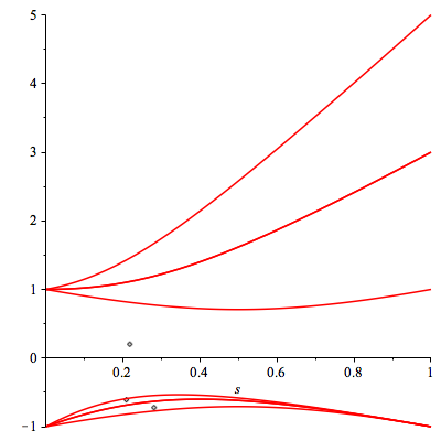
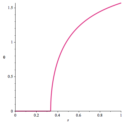
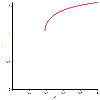
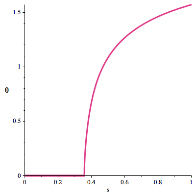
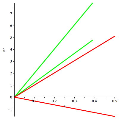
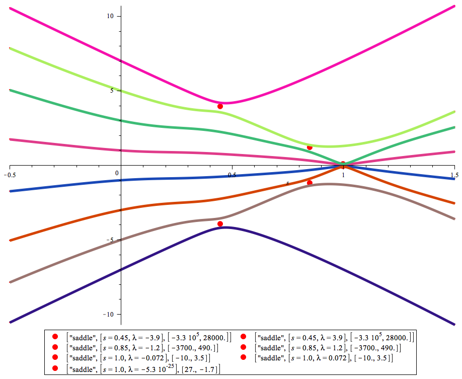
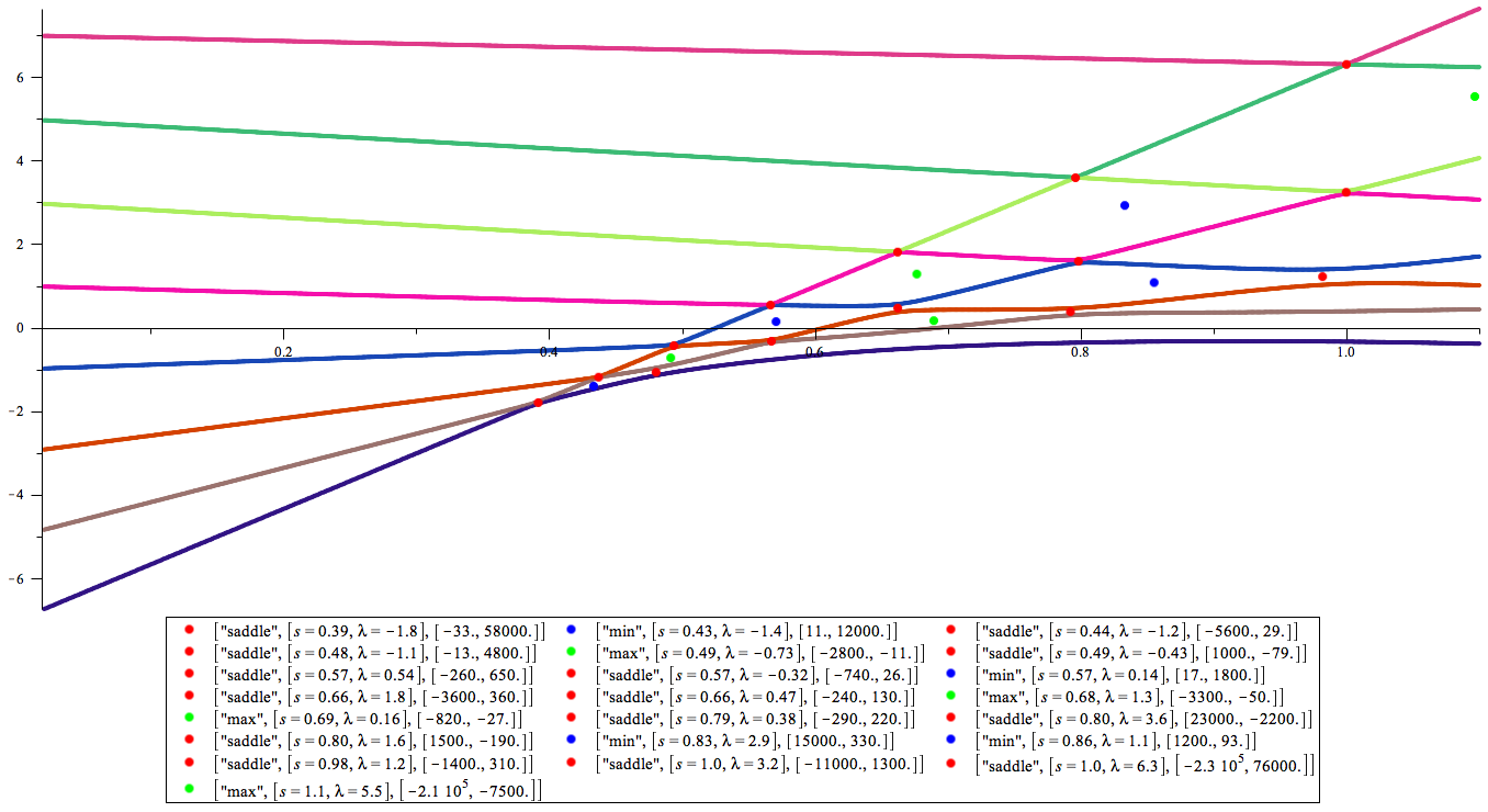
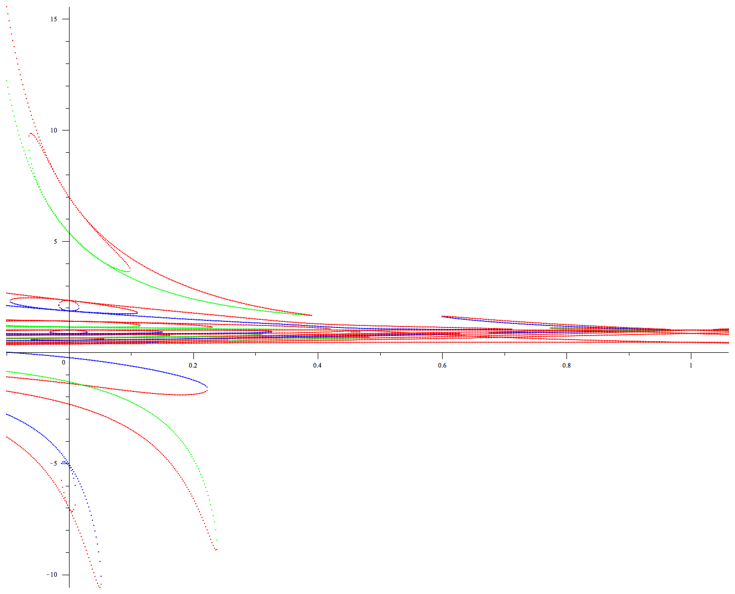
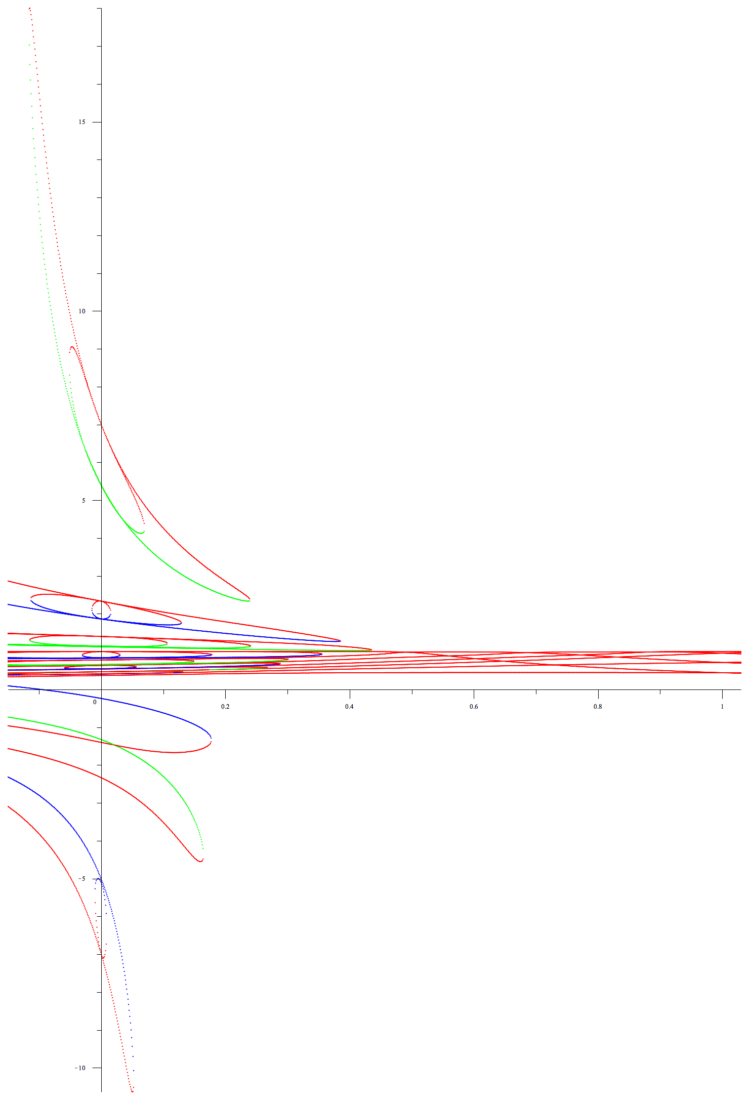
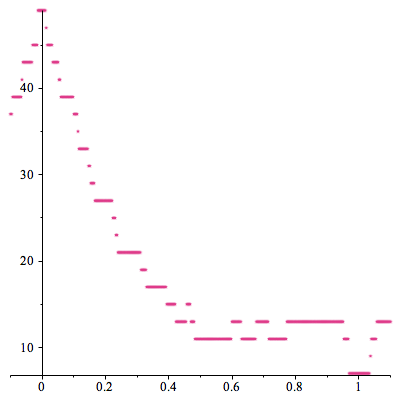
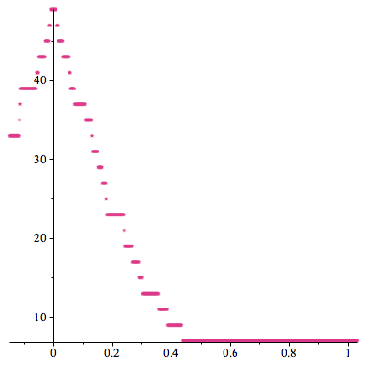
Other matrix elements are zero. Sending the non-stoquasticity parameter to zero amounts to the homotopical reduction of the angle described in the beginning. This pattern is reproduced in Figure 10 with the two lowest energies; see also Figure 9. Figure 11 shows how critical points are born and dead as changes without affecting the Euler characteristic. As the parameter decreases towards zero, the number of critical points increases, forcing the total curvature to redistribute itself on a larger set of critical points.
4 Conclusion
The paper presents a general methodology for enhancing the computational power of adiabatic quantum computations. The central idea is to homotopically deform the dynamics around the anti-crossing to weaken its effect. We have also illustrated the key role the Gauss-Bonnet theorem plays in this process. As illustrated by the two examples, the modifications provide speedup either by repelling the excited state or by transitioning from a first order QPT to the second, and so provide guidance on how to design enhancements. One interesting future direction is to perform such a deformation using degenerate critical points (hence, Conley theory [6]), as such points are no longer constrained by the Gauss-Bonnet theorem. This gives more freedom on how to control the evolution.
References
- [1] Augustin Banyaga and David Hurtubise. Lectures on Morse homology, volume 29 of Kluwer Texts in the Mathematical Sciences. Kluwer Academic Publishers Group, Dordrecht, 2004.
- [2] Victor Bapst and Guilhem Semerjian. On quantum mean-field models and their quantum annealing. Journal of Statistical Mechanics: Theory and Experiment, 2012(06):P06007, jun 2012.
- [3] Raoul Bott. Morse theory indomitable. Publications Mathématiques de l’IHÉS, 68:99–114, 1988.
- [4] Neil G Dickson. Elimination of perturbative crossings in adiabatic quantum optimization. New Journal of Physics, 13(7):073011, 2011.
- [5] Manfredo P. do Carmo. Differential geometry of curves and surfaces. Prentice-Hall, Inc., Englewood Cliffs, N.J., 1976. Translated from the Portuguese.
- [6] Raouf Dridi, Hedayat Alghassi, and Sridhar Tayur. Homological description of the quantum adiabatic evolution with a view toward quantum computations, ArXiv:1811.00675. 2018.
- [7] Raouf Dridi, Hedayat Alghassi, and Sridhar Tayur. Irreducible representations and Young diagrams for adiabatic quantum computations. In preparation. 2019.
- [8] Edward Farhi, Jeffrey Goldstone, Sam Gutmann, Joshua Lapan, Andrew Lundgren, and Daniel Preda. A quantum adiabatic evolution algorithm applied to random instances of an np-complete problem. Science, 292(5516):472–475, 2001.
- [9] F. Hund. Zur deutung der molekelspektren. i. Zeitschrift für Physik, 40(10):742–764, Oct 1927.
- [10] Hidetoshi Nishimori and Kabuki Takada. Exponential enhancement of the efficiency of quantum annealing by non-stoquastic hamiltonians. Frontiers in ICT, 4:2, 2017.
- [11] Jérémie Roland and Nicolas J. Cerf. Quantum search by local adiabatic evolution. Phys. Rev. A, 65:042308, Mar 2002.
- [12] Sei Suzuki, Jun ichi Inoue, and Bikas K. Chakrabarti. Quantum Ising Phases and Transitions in Transverse Ising Models. Springer Berlin Heidelberg, 2013.
- [13] Wim van Dam, Michele Mosca, and Umesh Vazirani. How powerful is adiabatic quantum computation? 2002.
- [14] J. von Neumann and E. P. Wigner. Über das Verhalten von Eigenwerten bei adiabatischen Prozessen, pages 294–297. Springer Berlin Heidelberg, Berlin, Heidelberg, 1993.