“Kepler Harmonies” and conformal symmetries

Abstract

Kepler’s rescaling becomes, when “Eisenhart-Duval lifted” to $5$-dimensional “Bargmann” gravitational wave spacetime, an ordinary spacetime symmetry for motion along null geodesics, which are the lifts of Keplerian trajectories. The lifted rescaling generates a well-behaved conserved Noether charge upstairs, which takes an unconventional form when expressed in conventional terms. This conserved quantity seems to have escaped attention so far. Applications include the Virial Theorem and also Kepler’s Third Law. The lifted Kepler rescaling is a Chrono-Projective transformation. The results extend to celestial mechanics and Newtonian Cosmology.

I Introduction

In today’s language, Kepler’s Third Law of planetary motion Harmonices states that the planetary trajectories are taken into themselves under the rescaling

$$t\to\Lambda^{3}\,t\,,\quad{\mathbf{x}}\to\Lambda^{2}\,{\mathbf{x}}\,,\quad\Lambda=\mathop{\rm const.}\nolimits$$ (I.1)

where $t$ denotes non-relativistic time and ${\mathbf{x}}$ the planet’s position. An intriguing feature is that the standard Lagrangian in $3+1$ non-relativistic dimensions changes under (I.1) as,

$${\mathcal{L}}_{Kepler}=\frac{m}{2}\left(\frac{d{{\mathbf{x}}}}{dt}\right)^{2}+\frac{GmM_{\odot}}{|{\mathbf{x}}|}\,\quad\to\quad\Lambda^{-2}\,{\mathcal{L}}_{Kepler}\,,$$ (I.2)

and is therefore not a symmetry in the sense that the Lagrangian does not change by a total derivative; some textbooks call it a “similitude” LLMech .

The aim of this Note is to celebrate the 400 years of Kepler’s “Harmonices Mundi” which first stated the Third Law Harmonices by providing new insight by “Eisenhart-Duval lifting” the problem to “Bargmann” space, which is in fact the space-time of a plane gravitational wave in 5-dimensions Eisenhart ; Bargmann ; DGH91 ; Brinkmann . The classical motions downstairs are the projections from the Bargmann space of null geodesics.

The clue is then that Kepler’s rescaling is a Chrono-Projective transformation DThese which becomes, when lifted to “Bargmann space”, a particular type of conformal isometry 5Chrono ; DGH91 , which acts as a perfectly well behaving symmetry for null geodesics “upstairs” and provides us with a perfectly well behaved conserved quantity however when expressed in terms of the original non-relativistic variables “downstairs”, this quantity takes an unconventional form.

II Kepler rescaling

Let us recall that the Bargmann manifold of a $(d,1)$ dimensional non-relativistic system is a $d+2$ dimensional manifold $\mathcal{M}$ endowed with a metric with Lorentz signature which also carries a covariantly constant null vector $\xi$ which we call here the “vertical vector”. In the case we are interested $d=3$ ; in suitable coordinates ${\mathbf{x}}\in{\mathbb{R}}^{3},t,s\in{\mathbb{R}}$, the metric and the vertical vector are,

$$g_{\mu\nu}dx^{\mu}dx^{\nu}=d{\bf x}^{2}+2dtds+\frac{2GM_{\odot}}{|{\mathbf{x}}|}dt^{2}\quad{\quad\text{and}\quad}\quad\xi={\partial}_{s}\,,$$ (II.1)

respectively. Moreover, $\Delta(\frac{1}{|{\mathbf{x}}|})=0$ for ${\mathbf{x}}\neq 0$ and therefore the metric is Ricci flat DGH91 ; Brinkmann — it is a vacuum solution of the Einstein equations. In other words, it is a gravitational wave in $5D$.

The geodesics in Bargmann space are described by the Lagrangian

$${\mathcal{L}}_{geo}=\frac{1}{2}(\dot{{\mathbf{x}}})^{2}+\dot{t}\dot{s}+\frac{GM_{\odot}}{|{\mathbf{x}}|}\,{\dot{t}}^{2}\,,$$ (II.2)

where the “dot”, $\dot{(\,\,)}=d/d\sigma$ is the derivative w.r.t. an affine parameter $\sigma$. Then (II.2) implies the equations of motion

$$\ddot{\mathbf{x}} =-GM_{\odot}{\dot{t}}^{2}\frac{{\mathbf{x}}}{|{\mathbf{x}}|^{3}}\,,$$ (II.3a)

$$\ddot{t} =0\,,$$ (II.3b)

$$\frac{\;d}{d\sigma}\big{(}\dot{s}+\frac{2GM_{\odot}}{\;|{\mathbf{x}}|}\,\dot{t}\big{)} =0\,.$$ (II.3c)

The non-relativistic spacetime is identified with the quotient of $\mathcal{M}$ by the integral curves of $\xi$; the non-relativistic motions — in our case the Kepler orbits — are the projections to non-relativistic space-time of the null geodesic of the $5$ dimensional metric (II.1).

Chrono-Projective transformations were introduced originally in the Newton-Cartan context DThese . In Bargman terms they are conformal mapping of $\mathcal{M}$, $f^{*}g_{\mu\nu}=\Omega^{2}(t)g_{\mu\nu}$, which leave the direction of $\xi$ invariant 5Chrono . Working infinitesimally,

$$L_{Y}g_{\mu\nu}=2\omega(t)\,g_{\mu\nu}\,{\quad\text{and}\quad}L_{Y}\xi=\psi(t)\,\xi\,.$$ (II.4)

Lifting the Kepler rescaling (I.1) to $5D$ Bargmann space as

$$t\to\Lambda^{3}\,t\,,\;\;{\mathbf{x}}\to\Lambda^{2}\,{\mathbf{x}}\,,\;\;s\to\Lambda\,s$$ (II.5a)

$$Y=3t\,{\partial}_{t}+2{\mathbf{x}}\,{\partial}_{{\mathbf{x}}}+s\,{\partial}_{s}$$ (II.5b)

rescales the metric conformally, $g_{\mu\nu}dx^{\mu}dx^{\nu}\to\Lambda^{4}\,g_{\mu\nu}dx^{\mu}dx^{\nu}\,.$ It does not preserve $\xi$, though, only its direction,

$${\partial}_{s}\to\Lambda^{-1}{\partial}_{s}\,,\quad\text{i.e.}\quad L_{Y}{\partial}_{s}=-{\partial}_{s}\,,$$ (II.6)

and is therefore Chrono-Projective. The geodesic Lagrangian (II.2) scales, under the lifted Kepler scaling (II.5), as ${\mathcal{L}}_{geo}\to\Lambda^{4}{\mathcal{L}}_{geo}\,.$ At the first sight, this appears to be a no better behaviour than “downstairs”, (I.2), – and this is indeed so when the geodesic is timelike or spacelike. However for null geodesics the Lagrangian is constrained to vanish,

$${\mathcal{L}}_{geo}=0,$$ (II.7)

which makes it invariant : lifted Kepler rescalings act, for null geodesics, as symmetries.

Let us emphasise that “upstairs” i.e., in the $5D$ gravitational wave space-time, no additional constraint is required; Noether’s theorem works for any conformal vectorfield which leaves the geodesic Lagrangian invariant. The associated conserved quantity for motion along a null geodesic in $5D$ is, in our case,

$$\;\;\displaystyle{{\mathcal{Q}}=3tp_{t}+2x^{i}p_{i}+sp_{s}\,,}\;\;$$ (II.8)

whose conservation can also be checked by a direct calculation : in terms of the canonical momenta the eqns of motion (II.3) imply that $p_{t}=\dot{s}+\frac{2GM_{\odot}}{|{\mathbf{x}}|}\,\dot{t}$ and $p_{s}=\dot{t}$ are constants of the motion. Then deriving ${\mathcal{Q}}$ and using the eqns of motion we get

$$\dot{{\mathcal{Q}}}=4{\mathcal{L}}_{geo}=0\,,$$ (II.9)

because, precisely, our geodesics are null. Conversely, the generating vector field $Y$ in (II.5b) is recovered as $Y^{\mu}=\Big{\{}x^{\mu},{\mathcal{Q}}\Big{\}}={{\partial}{\mathcal{Q}}}/{{\partial}p_{\mu}}\,.$

The geodesic Hamiltonian is

$${\mathcal{H}}_{geo}=\frac{1}{2}{p_{i}p_{i}}-\frac{GM_{\odot}}{|{\mathbf{x}}|}p_{s}^{2}+p_{t}p_{s}.$$ (II.10)

Performing a Legendre transformation, this Hamiltonian becomes the geodesic Lagrangian, ${\mathcal{H}}_{geo}={\mathcal{L}}_{geo}$. Moreover, identifying $p_{s}$ with $m$ the mass in $3D$ and expressing $p_{t}$ from the null condition ${\mathcal{H}}_{geo}=0$ yields

$$p_{t}=-\left(\frac{1}{2m}p_{i}p_{i}-\frac{GmM_{\odot}}{|{\mathbf{x}}|}\right)=-E\,,$$ (II.11)

which is (minus) the non-relativistic energy. Then from $\dot{t}=p_{s}=m$ we infer that $d/d\sigma=md/dt$. Denoting $d/dt$ by “prime”, $p_{i}=m(x^{i})^{\prime}$ and putting the geodesic Lagrangian equal to zero yields

$${s}^{\prime}(t)=-\left(\frac{1}{2}({\mathbf{x}}^{\prime})^{2}+\frac{GM_{\odot}}{|{\mathbf{x}}|}\right)=-\frac{1}{m}{\mathcal{L}}_{Kepler}\,.$$ (II.12)

The change of $s$ along a lightlike geodesic is thus proportional to minus the 3D Kepler action calculated along the projected trajectory Brinkmann  ,

$$s(t)=\frac{{\mathcal{Q}}}{m}+3t\frac{E}{m}-\frac{2(p_{i}x^{i})}{m}=s_{0}-\frac{1}{m}\int_{0}^{t}\!{\mathcal{L}}_{Kepler}({\mathbf{x}}(\tau),{\mathbf{x}}^{\prime}(\tau))\,d\tau\,.$$ (II.13)

The conserved quantity (II.8) can be expressed “mostly” but not completely in $3D$ terms,

$${\mathcal{Q}}=-3tE+m\frac{\;\,d}{dt}(x_{i}x^{i})-\int_{0}^{t}\!\!{\mathcal{L}}_{Kepler}({\mathbf{x}}(\tau),{\mathbf{x}}^{\prime}(\tau))\,d\tau\,+ms_{0}\,,$$ (II.14)

which explains also why it does not project down : it depends on $s_{0}$. However subtracting $ms_{0}$, we get $Q_{Kepler}={\mathcal{Q}}-ms_{0}$

$$\framebox{$\;\displaystyle{Q_{Kepler}=-3tE+m\frac{\;\,d}{dt}(x_{i}x^{i})-\int_{0}^{t}\!\!\!{\mathcal{L}}_{Kepler}({\bf x}(\tau),{\bf x}^{\prime}(\tau))\,d\tau}\;$}\quad$$ (II.15)

where the integration is along the classical trajectory in $3$-space. $Q_{Kepler}$ is well-defined and also conserved, as proved along the same lines as for (II.9)). We mention that the same expression can also be derived from the original Kepler Lagrangian using a generalization of the classical Noether theorem Kosinskietal .

Let us stress that (II.15) is a local quantity despite its surprising form, because the classical trajectory (apart at caustic singularities) is uniquely deteremined by its end points. The integral is just Hamilton’s action function.

For $t=0$ both the first and the last terms in (II.15) vanish, leaving us with $Q_{Kepler}=2p_{i}(0)x^{i}(0)\,.$ Let us record for further reference that $\displaystyle\int_{0}^{t}\!{\mathcal{L}}_{Kepler}\,dt=\displaystyle\int_{0}^{t}\!p_{i}dx^{i}-Et$, which allows us to rewrite (II.15) also as

$$Q_{Kepler}=-2tE+m\frac{\;\,d}{dt}(x_{i}x^{i})-\int_{0}^{t}\!\!\!p_{i}\frac{dx^{i}}{dt}\,dt\,.$$ (II.16)

III Applications of our conserved quantity

We restrict our attention henceforth to elliptic motions in the $x_{3}=0$ plane with $E<0$ and draw some interesting consequences of the conservation of (II.15). Parabolic and hyperbolic motions behave similarly.

If time is measured so that for $t=0$ we are in the closest (perihelion) position then $Q_{Kepler}$ is just zero. But then a full period later i.e. for $t=T$, we are back where we started from, so that $\big{(}d(x_{i}x^{i})/dt\big{)}(t=T)=0$, yielding,

$$2TE+\int_{0}^{T}\!\!\!p_{i}\frac{dx^{i}}{dt}\,dt=0\,.$$ (III.1)

The first consequence is that expressing the momenta in terms of velocities allows us to infer the Virial Theorem : the energy is minus the average kinetic energy for a full period,

$$E=-\frac{1}{T}\int_{0}^{T}\frac{m}{2}(\frac{d{\bf x}}{dt})^{2}dt=-\overline{E}_{k}\,.$$ (III.2)

The integral in (III.1) can actually be determined. Consider the radius vectors drawn from the focus where the Sun sits and also from the other focus to the current position of the planet. The rates of change of the areas swept out the by these two radius vectors are

$$\frac{dA}{dt} =\frac{1}{2m}p_{\phi}\,,$$ (III.3a)

$$\frac{dA^{\prime}}{dt} =\frac{b^{2}}{2p_{\phi}}\bigl{(}p_{r}\frac{dr}{dt}+p_{\phi}\frac{d\phi}{dt}\bigr{)}\,.$$ (III.3b)

where $p_{\phi}$ is the angular momentum. The first of these relations is Kepler’s Second Law, while (III.3b) might reasonably be called Tait’s Law Tait ; TaitSteele ; see GEllis2 for a new, geometric proof. Then for a full period $T$ both radius vectors sweep through the ellipse, and therefore,

$$\pi ab=\left\{\begin{array}[]{lll}\displaystyle\int_{0}^{T}\frac{dA}{dt}dt&=&\displaystyle\frac{p_{\phi}}{2m}\,T\,,\\[20.0pt] \displaystyle\int_{0}^{T}\frac{dA^{\prime}}{dt}dt&=&\displaystyle\frac{b^{2}}{2p_{\phi}}\int_{0}^{T}\!\bigl{(}p_{r}\frac{dr}{dt}+p_{\phi}\frac{d\phi}{dt}\bigr{)}dt\,,\end{array}\right.$$ (III.4)

where $a$ and $b$ are the semi-major and the semi-minor axes, respectively. From here we infer

$$\int_{0}^{T}\!\bigl{(}p_{r}\frac{dr}{dt}+p_{\phi}\frac{d\phi}{dt}\bigr{)}dt=\frac{4\pi^{2}a^{2}m}{T}\,.$$ (III.5)

Reinserting this into (III.1) and using $E=-GmM_{\odot}/2a$, we end up with the Third Law,

$$\frac{a^{3}}{T^{2}}=\frac{GM_{\odot}}{4\pi^{2}}\,.$$ (III.6)

Let us observe finally that while the planet goes around once the vertical coordinate changes, by (II.13), by

$$\Delta s=-\frac{1}{m}\int_{0}^{T}\!\!{\mathcal{L}}_{Kepler}dt=-\frac{1}{m}\int_{0}^{T}\!\bigl{(}p_{r}\frac{dr}{dt}+p_{\phi}\frac{d\phi}{dt}\bigr{)}dt+\frac{E}{m}T=-\frac{4\pi^{2}a^{2}}{T}-\frac{GM_{\odot}T}{2a}.$$ (III.7)

The equations of motion (II.3) can be solved numerically ; it confirms that (II.8) is indeed conserved, and also the formulae of this section. The solutions are shown in Fig.1.

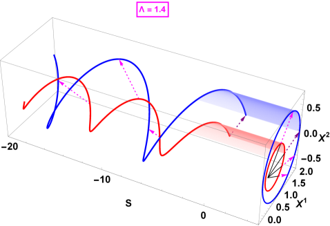
Figure 1: The closed Keplerian trajectories become spirals when lifted to Bargmann space. They are permuted by the lift (II.5) of Kepler’s rescaling (I.1) indicated by arrows.

IV Generalization to $N$ bodies

The Kepler’s scaling property holds in fact for all of Newtonian Cosmology GEllis ; GEllis2 . The $N$-body equations (No sum on $a$),

$$m_{a}\frac{d^{2}{\bf x}_{a}}{dt^{2}}=-\sum_{b\neq a}m_{a}m_{b}\frac{{\bf x}_{a}-{\bf x}_{b}}{\,|{\bf x}_{a}-{\bf x}_{b}|^{3}},\qquad a=1,2,\dots,N$$ (IV.1)

correspond, in the Bargmann framework, to the projections to the $N$-particle configuration space of the null geodesics of the $3N+2$ dimensional metric DGH91 ,

$$g_{\mu\nu}dx^{\mu}dx^{\nu}=\sum_{a=1}^{N}\frac{m_{a}}{m}d{\bf x}_{a}^{2}+2dtds-\frac{2U}{m}dt^{2}\,,$$ (IV.2a)

$$m=\sum_{a}m_{a}\,,\qquad U=-\frac{1}{2}\sum_{a,b\neq a}\frac{Gm_{a}m_{b}}{|{\bf x}_{a}-{\bf x}_{b}|}\,.$$ (IV.2b)

Then the Kepler rescaling (II.5), $t\to\Lambda^{3}t,\,{\bf x}_{a}\to\Lambda^{2}\,{\bf x}_{a},\,s\to\Lambda\,s$, acts plainly conformally, $g_{\mu\nu}dx^{\mu}dx^{\nu}\to\Lambda^{4}g_{\mu\nu}dx^{\mu}dx^{\nu}$, generating a symmetry and a conserved charge for null geodesics,

$${\mathcal{Q}}=-3TE+2\sum_{a}{\bf x}_{a}\cdot{\bm{p}}_{a}+sm\,,\qquad E=\sum_{a}\frac{{\bm{p}}_{a}^{2}}{2m_{a}}+U\,,$$ (IV.3a)

$$s=s_{0}-\frac{1}{m}\int_{0}^{t}\!\!{\mathcal{L}}_{N}d\tau\,,\qquad\qquad\qquad\;\;{\mathcal{L}}_{N}=\sum_{a}\frac{m_{a}({\bf x}_{a}^{\prime})^{2}}{2}-U\,.$$ (IV.3b)

Here ${\mathcal{L}}_{N}$ is the $N$-body Lagrangian. This charge projects again to a conserved charge of unconventional form.

V Conclusion

This year we celebrate the 400’th anniversary of Kepler’s discovery of his Third Law of planetary motion, which concerns the period and size of geometrically similar bound orbits Harmonices .

Famously, Newton derived this and other properties of the orbits from his Universal Inverse Square Law of Gravitation. This is what we find in most textbooks, e.g. in LLMech . Since his time there have been many investigations of the geometry and symmetry of these orbits, but none has derived Kepler’s Third Law using the methods introduced by Emmy Noether.

In this paper we start with a previously developed but not well known general formalism called the Bargmann framework of Eisenhart Eisenhart , and of Duval et al Bargmann ; DGH91 . It states that the motion may be regarded as the projection of the motion of light rays moving in a five-dimensional extended spacetime and obtain for the first time Kepler’ law as a consequence of Emmy Noether’s theorem.

In detail, lifting Kepler’s rescaling, (I.1), to $5D$ Bargmann space as (II.5) generates there a well-behaved conserved charge, (II.8), for null geodesics. It allows us to integrate the “vertical” motion once the Kepler motions had been determined. Subtracting a constant term yields a conserved charge for ordinary planetary motion of an unconventional form . Rather incredibly, (II.15) appears to be a new conserved quantity which seems to have escaped attention so far. It is in fact different from the familiar Runge-Lenz vector as can be understood by recalling their origin: while (II.8) is a scalar generated by a conformal Killing vector of 5D Bargmann space, the components of the Runge-Lenz vector are associated with 3 Killing tensors DGH91 .

The conserved quantity (II.15) allows us to derive the Virial Theorem, (III.2), the usual form of Kepler’s Third law, (III.6); the evolution of the $s$-coordinate is consistent with Fig.1.

One can inquire if the Kepler problem admits further spacetime symmetries. The answer is no: the intrinsically defined Newton-Cartan structure allows for a $5$-parameter Chrono-Projective group only, composed by rotations, time translations and the Kepler rescaling DThese . For further details and applications of conformal symmetries for gravitational waves, see AndrPrenc ; Conf4GW . Other examples of Chrono-Projective transformations include the Schrödinger-Newton equations DuLaz , hydrodynamics hydro , Schrödinger operators Gundry and projective dynamics Cariglia15 .

The expression $\displaystyle\int_{0}^{T}\!\!\!p_{i}\frac{dx^{i}}{dt}\,dt$ we used repeatedly in sec.III had actually played a prominent rôle in the Old Quantum Theory, namely in the Nicholson-Bohr-Wilson-Sommerfeld quantization conditions Nicholson ; Bohr ; Wilson ; Sommerfeld ; Wilson2  : if a coordinate $q$ varies periodically with time, then the quantity

$$\frac{1}{2\pi h}\oint pdq\,,$$ (V.1)

where $h=2\pi\hbar$ is Planck’s constant, should be an integer. For the closed Keplerian orbits we have two such coordinates, $r$ and $\phi$. We have in particular the quantization of angular momentum first suggested by Nicholson Nicholson and its generalization proposed, independently, by Bohr Bohr , Wilson Wilson ; Wilson2 and by Sommerfeld Sommerfeld ,

$$\frac{1}{2\pi h}\oint p_{\phi}d\phi=l\,,{\quad\text{and}\quad}\frac{1}{2\pi{h}}\oint(p_{r}dr+p_{\phi}d\phi)=n\,,$$ (V.2)

where $l$ the total angular momentum and $n$ is the principal quantum number, respectively. The geometrical significance of these relations is given by (III.3b).

In our study we were helped by that, because of the Equivalence Principle, the Keplerian trajectories are independent of the mass. However, it is illuminating to consider the 3D transformations inherited from those in 5D phase space and generated by (II.8) by complementing (I.1) with $m\rightarrow\Lambda^{-1}m\,.$ Details will be discussed elsewhere.

We conclude with the remark that Kepler’s game changing three laws remain as relevant to our exploration of the universe and the laws that govern it today as when they were first formulated. No better illustration of this fact may be found than in Gillessen:2008qv ; Takekawa . Studying the motion of matter around a black hole could provide a test for the validity/corrections of Kepler’s laws at the large scale.

Note added. After our paper was submitted, we came across Keplar which has a vague relation to our work here.

- (1) J. Kepler, “Ioannis Keppleri Harmonices mundi libri V.” Linz, (Austria): Johann Planck, 1619, p. 189. According to Wikipedia: https://en.wikipedia.org/wiki/Harmonices- Mundi#cite-note-2 From the bottom of p. 189: “…proportio qua est inter binorum quorumcunque Planetarum tempora periodica, sit praecise sesquialtera proportionis mediarum distantiarum …” (the proportion between the periodic times of any two planets is precisely the sesquialternate proportion [i.e., the ratio of 3:2] of their mean distances …). An English translation of Kepler’s Harmonices Mundi is available as: Johannes Kepler with E.J. Aiton, A.M. Duncan, and J.V. Field, trans., The Harmony of the World (Philadelphia, Pennsylvania: American Philosophical Society, 1997); see especially p. 411.
- (2) L. Landau and E. Lifchitz, Physique Théorique, Tome I: Mécanique. édition. Éditions MIR, Moscou (1969); V. Arnold, Les méthodes mathématiques de la mécanique classique, Éditions MIR, Moscou (1976); H. Goldstein, Classical Mechanics, 2nd ed. Addison-Wesley (1980).
- (3) L. P. Eisenhart, “Dynamical trajectories and geodesics”, Annals Math. 30 591-606 (1928).
- (4) C. Duval, G. Burdet, H. P. Künzle and M. Perrin, “Bargmann structures and Newton-Cartan theory”, Phys. Rev. D 31 (1985) 1841;
- (5) C. Duval, G.W. Gibbons, P. Horvathy, “Celestial mechanics, conformal structures and gravitational waves,” Phys. Rev. D43 (1991) 3907. [hep-th/0512188].
- (6) M. W. Brinkmann, “Einstein spaces which are mapped conformally on each other,” Math. Ann. 94 (1925) 119.
- (7) C. Duval, “Quelques procédures géométriques en dynamique des particules,” Doctorat d’Etat ès Sciences (Aix-Marseille-II), 1982 (unpublished). See also C. Duval, “Sur la géométrie Chrono-Projective de l’espace-temps classique,” in Actes des Journées relativistes de Lyon, (1982), and G. Burdet, C. Duval and M. Perrin, “Cartan Structures On Galilean Manifolds: The Chrono-Projective Geometry,” J. Math. Phys. 24 (1983) 1752. doi:10.1063/1.525927.
- (8) M. Perrin, G. Burdet and C. Duval, “Chrono-Projective Invariance of the Five-dimensional Schrödinger Formalism,” Class. Quant. Grav. 3 (1986) 461. doi:10.1088/0264-9381/3/3/020
- (9) P.-M. Zhang, M. Elbistan, P. A. Horvathy and P. Kosinski, “A generalized Noether theorem for scaling symmetry,” arXiv:1903.05070 [math-ph].
- (10) P. G. Tait, “Note on Action,” Proc. R. Soc. Edinburgh, Session 1864-65. p. 404 (1865). doi:10.1017/S0370164600040992
- (11) P.G. Tait and W. J. Steele, A Treatise on Dynamics of a Particle, MacMillan and Co. Ltd, London and New York. Seventh edition (1900).
- (12) G. F. R. Ellis and G. W. Gibbons, “Discrete Newtonian Cosmology: Perturbations,” Class. Quant. Grav. 32 (2015) no.5, 055001 doi:10.1088/0264-9381/32/5/055001 [arXiv:1409.0395 [gr-qc]].
- (13) G. F. R. Ellis and G. W. Gibbons, “Discrete Newtonian Cosmology,” Class. Quant. Grav. 31 (2014) 025003 doi:10.1088/0264-9381/31/2/025003 [arXiv:1308.1852 [astro-ph.CO]].
- (14) N. Dimakis, P. A. Terzis and T. Christodoulakis, “Integrability of geodesic motions in curved manifolds through non-local conserved charges,” arXiv:1901.07187 [gr-qc]. 1901.07187
- (15) K. Andrzejewski and S. Prencel, “Memory effect, conformal symmetry and gravitational plane waves,” Phys. Lett. B 782 (2018) 421 doi:10.1016/j.physletb.2018.05.072 [arXiv:1804.10979 [gr-qc]].
- (16) P.-M. Zhang, M. Cariglia, M. Elbistan, G. W. Gibbons and P. A. Horvathy, “Scaling and conformal symmetries for plane gravitational waves” (work in progress).
- (17) C. Duval and S. Lazzarini, “On the Schrödinger-Newton equation and its symmetries: a geometric view,” Class. Quant. Grav. 32 (2015) no.17, 175006 doi:10.1088/0264-9381/32/17/175006 [arXiv:1504.05042 [math-ph]].
- (18) M. Hassaine and P. A. Horvathy, “Symmetries of fluid dynamics with polytropic exponent,” Phys. Lett. A 279 (2001) 215 doi:10.1016/S0375-9601(00)00834-3 [hep-th/0009092]; P. A. Horvathy and P.-M. Zhang, “Non-relativistic conformal symmetries in fluid mechanics,” Eur. Phys. J. C 65 (2010) 607 doi:10.1140/epjc/s10052-009-1221-x [arXiv:0906.3594 [physics.flu-dyn]].
- (19) J. Gundry, “Higher symmetries of the Schrödinger operator in Newton-Cartan geometry,” J. Geom. Phys. 113 (2017) 73 doi:10.1016/j.geomphys.2016.06.003 [arXiv:1601.02797 [math-ph]].
- (20) M. Cariglia, “Null lifts and projective dynamics,” Annals Phys. 362 (2015) 642 doi:10.1016/j.aop.2015.09.002 [arXiv:1506.00714 [math-ph]].
- (21) J.W. Nicholson, “The Constitution of the Solar Corona. IL ,” Mon. Not. R.A.S. 72, 677-693, (1912) https://doi.org/10.1093/mnras/72.8.677 .
- (22) N. Bohr, “On the Constitution of Atoms and Molecules”, Parts I, II, III. Phil. Mag. 26 1, 476, 857 (1913)
- (23) W. Wilson, “The quantum-theory of radiation and line spectra,” Phil. Mag. 29, 795 (1915)
- (24) W. Wilson, A Hundred Years of Physics, Gerald Duckworth and Sons td London (1950)
- (25) A. Sommerfeld, “Zur Quantentheorie der Spektrallinien,” Ann. der Phys. 51, 1-94 (1916)
- (26) S. Gillessen, F. Eisenhauer, S. Trippe, T. Alexander, R. Genzel, F. Martins and T. Ott, “Monitoring stellar orbits around the Massive Black Hole in the Galactic Center,” Astrophys. J. 692 (2009) 1075 doi:10.1088/0004-637X/692/2/1075 [arXiv:0810.4674 [astro-ph]].
- (27) S. Takekawa et al. “Indication of Another Intermediate-mass Black Hole in the Galactic Center,” Astrophysical Journal Letters 871:L1 (2019)
- (28) N. Ogawa, “A Note on the scale symmetry and Noether current,” hep-th/9807086.