An Optimistic Acceleration of AMSGrad for Nonconvex Optimization

Abstract

We propose a new variant of AMSGrad [32], a popular adaptive gradient based optimization algorithm widely used for training deep neural networks. Our algorithm adds prior knowledge about the sequence of consecutive mini-batch gradients and leverages its underlying structure making the gradients sequentially predictable. By exploiting the predictability and ideas from optimistic online learning, the proposed algorithm can accelerate the convergence and increase sample efficiency. After establishing a tighter upper bound under some convexity conditions on the regret, we offer a complimentary view of our algorithm which generalizes the offline and stochastic version of nonconvex optimization. In the nonconvex case, we establish a non-asymptotic convergence bound independently of the initialization. We illustrate the practical speedup on several deep learning models via numerical experiments.

1 Introduction

Deep learning models have been successful in several applications, from robotics (e.g., [22]), computer vision (e.g., [19, 16]), reinforcement learning (e.g., [27]) and natural language processing (e.g., [17]). With the sheer size of modern datasets and the dimension of neural networks, speeding up training is of utmost importance. To do so, several algorithms have been proposed in recent years, such as AMSGrad [32], Adam [20], RMSPROP [36], AdADELTA [42], NADAM [11], Local Adam [5], SAGD [44], etc. All the prevalent algorithms for training deep networks mentioned above combine two ideas: the idea of adaptivity from AdaGrad [25, 12] and the idea of momentum from Nesterov’s Method [29] or Heavy ball method [30]. AdaGrad is an online learning algorithm that works well compared to the standard online gradient descent when the gradient is sparse. Its update has a notable feature: it leverages an anisotropic learning rate depending on the magnitude of the gradient for each dimension which helps in exploiting the geometry of the data. On the other hand, Nesterov’s Method or Heavy ball Method [30] is an accelerated optimization algorithm which update not only depends on the current iterate and gradient but also depends on the past gradients (i.e., momentum). State-of-the-art algorithms such as AMSGrad [32] and Adam [20] leverage these ideas to accelerate the training of nonconvex objective functions, for instance deep neural networks losses.

In this paper, we propose an algorithm that goes beyond the hybrid of the adaptivity and momentum approach. Our algorithm is inspired by Optimistic Online learning [8, 31, 35, 1, 26], which assumes that, in each round of online learning, a predictable process of the gradient of the loss function is available. Then, an action is played exploiting these predictors. By capitalizing on this (possibly) arbitrary process, algorithms in Optimistic Online learning enjoy smaller regret than the ones without gradient predictions. We combine the Optimistic Online learning idea with the adaptivity and the momentum ideas to design a new algorithm — OPT-AMSGrad.

A single work along that direction stands out. [9] develop Optimistic-Adam leveraging optimistic online mirror descent [31]. Yet, Optimistic-Adam is specifically designed to optimize two-player games, e.g., GANs [16] which is in particular a two-player zero-sum game. There have been some related works in Optimistic Online learning [8, 31, 35] showing that if both players use an Optimistic type of update, then accelerating the convergence to the equilibrium of the game is possible. [9] build on these related works and show that Optimistic-Mirror-Descent can avoid the cycle behavior in a bilinear zero-sum game accelerating the convergence. In contrast, in this paper, the proposed algorithm is designed to accelerate nonconvex optimization (e.g., empirical risk minimization). To the best of our knowledge, this is the first work exploring towards this direction and bridging the unfilled theoretical gap at the crossroads of online learning and stochastic optimization.

The contributions of this paper are as follows:

• We derive an optimistic variant of AMSGrad borrowing techniques from online learning procedures. Our method relies on (I) the addition of prior knowledge in the sequence of model parameter estimates leveraging a predictable process able to provide guesses of gradients through the iterations; (II) the construction of a double update algorithm done sequentially. We interpret this two-projection step as the learning of the global parameter and of an underlying scheme which makes the gradients sequentially predictable.

• We focus on the theoretical justifications of our method by establishing novel non-asymptotic and global convergence rates in both convex and nonconvex cases. Based on convex regret minimization and nonconvex stochastic optimization views, we prove, respectively, that our algorithm suffers regret of $\mathcal{O}(\sqrt{\sum_{t=1}^{T}\|g_{t}-m_{t}\|^{2}_{\psi_{t-1}}})$ and achieves a convergence rate $\mathcal{O}(\sqrt{d/T}+d/T)$, where $g_{t}$ is the gradient, $m_{t}$ is its prediction, $d$ is the dimension of the problem and $T$ the total number of iterations.

The proposed algorithm adapts to the informative dimensions, exhibits momentum, and also exploits a good guess of the next gradient to facilitate acceleration. Besides the complete convergence analysis of OPT-AMSGrad, we conduct numerical experiments and show that the proposed algorithm not only accelerates the training procedure, but also leads to better empirical generalization performance.

Notations: We follow the notations of adaptive optimization [20, 32]. For any $u$, $v\in\mathbb{R}^{d}$, $u/v$ represents the element-wise division, $u^{2}$ the element-wise square, $\sqrt{u}$ the element-wise square-root. We denote $g_{1:T}[i]$ as the sum of the $i_{th}$ element of $g_{1},\dots,g_{T}\in\mathbb{R}^{d}$ and $\|\cdot\|$ as the Euclidean norm.

2 Preliminaries

We begin by providing some background on both online learning and adaptive methods.

Optimistic Online learning.  The standard setup of Online learning is that, in each round $t$, an online learner selects an action $w_{t}\in\Theta\subseteq\mathbb{R}^{d}$, observes $\ell_{t}(\cdot)$ and suffers the associated loss $\ell_{t}(w_{t})$ after the action is committed. The goal of the learner is to minimize the regret,

$$\mathcal{R}_{T}(\{w_{t}\}):=\sum_{t=1}^{T}\ell_{t}(w_{t})-\sum_{t=1}^{T}\ell_{t}(w^{*})\;,$$

which is the cumulative loss of the learner minus the cumulative loss of some benchmark $w^{*}\in\Theta$. The idea of Optimistic Online learning (e.g., [8, 31, 35, 1]) is as follows. In each round $t$, the learner exploits a guess $m_{t}(\cdot)$ of the gradient $\nabla\ell_{t}(\cdot)$ to choose an action $w_{t}$. Consider the Follow-the-Regularized-Leader (FTRL, [18]) online learning algorithm which update reads

$$\textstyle w_{t}=\arg\min_{w\in\Theta}\langle w,L_{t-1}\rangle+\frac{1}{\eta}\textsf{R}(w)\;,$$

where $\eta$ is a parameter, $\textsf{R}(\cdot)$ is a $1$-strongly convex function with respect to a given norm on the constraint set $\Theta$, and $L_{t-1}:=\sum_{s=1}^{t-1}g_{s}$ is the cumulative sum of gradient vectors of the loss functions up to round $t-1$. It has been shown that FTRL has regret at most $\mathcal{O}(\sqrt{\sum_{t=1}^{T}\|g_{t}\|_{*}^{2}})$. The update of its optimistic variant, called Optimistic-FTRL and developed in [35] reads

$$\textstyle w_{t}=\arg\min_{w\in\Theta}\langle w,L_{t-1}+m_{t}\rangle+\frac{1}{\eta}\textsf{R}(w)\;,$$

where $\{m_{t}\}_{t>0}$ is a predictable process incorporating (possibly arbitrary) knowledge about the sequence of gradients $\{g_{t}:=\nabla\ell_{t}(w_{t})\}_{t>0}$. Under the assumption that the loss functions are convex, it has been shown in [35] that the regret of Optimistic-FTRL is at most $\mathcal{O}(\sqrt{\sum_{t=1}^{T}\|g_{t}-m_{t}\|_{*}^{2}})$.

Remark: Note that the usual worst-case bound is preserved even when the predictors $\{m_{t}\}_{t>0}$ do not predict well the gradients. Indeed, if we take the example of Optimistic-FTRL, the bound reads $\sqrt{\sum_{t=1}^{T}\|g_{t}-m_{t}\|_{*}^{2}}\leq 2\max\limits_{w\in\Theta}\|\nabla\ell_{t}(w)\|\sqrt{T}$ which is equal to the usual bound up to a factor $2$ [31], under certain boundedness assumptions on $\Theta$ detailed below. Yet, when the predictors $\{m_{t}\}_{t>0}$ are well designed, the resulting regret will be lower. We will have a similar argument when comparing OPT-AMSGrad and AMSGrad regret bounds in Section 4.1.

We emphasize, in Section 3, the importance of leveraging a good guess $m_{t}$ for updating $w_{t}$ in order to get a fast convergence rate (or equivalently, small regret) and introduce in Section 6 a simple predictable process $\{m_{t}\}_{t>0}$ leading to empirical acceleration on various applications.

Adaptive optimization methods.  Adaptive optimization has been popular in various deep learning applications due to their superior empirical performance. Adam [20], a popular adaptive algorithm, combines momentum [30] and anisotropic learning rate of AdaGrad [12]. More specifically, the learning rate of AdaGrad at time $T$ for dimension $j$ is proportional to the inverse of $\sqrt{\Sigma_{t=1}^{T}g_{t}[j]^{2}}$, where $g_{t}[j]$ is the $j$-th element of the gradient vector $g_{t}$ at time $t$. This adaptive learning rate helps accelerating the convergence when the gradient vector is sparse [12], yet, when applying AdaGrad to train deep neural networks, it is observed that the learning rate might decay too fast, see [20] for more details. Therefore, [20] put forward Adam that uses a moving average of the gradients divided by the square root of the second moment of this moving average (element-wise multiplication), for updating the model parameter $w$. A variant, called AMSGrad and detailed in Algorithm 1, has been developed in [32] to fix Adam failures.

Algorithm 1 AMSGrad [32]

1:  Required: parameter $\beta_{1}$, $\beta_{2}$, and $\eta_{t}$.

2:  Init: $w_{1}\in\Theta\subseteq\mathbb{R}^{d}$ and $v_{0}=\epsilon 1\in\mathbb{R}^{d}$.

3:  for $t=1$ to $T$ do

4:     Get mini-batch stochastic gradient $g_{t}$ at $w_{t}$.

5:     $\theta_{t}=\beta_{1}\theta_{t-1}+(1-\beta_{1})g_{t}$.

6:     $v_{t}=\beta_{2}v_{t-1}+(1-\beta_{2})g_{t}^{2}$.

7:     $\hat{v}_{t}=\max(\hat{v}_{t-1},v_{t})$.

8:     $w_{t+1}=w_{t}-\eta_{t}\frac{\theta_{t}}{\sqrt{\hat{v}}_{t}}$. (element-wise division)

9:  end for

The difference between Adam and AMSGrad lies in line 7 of Algorithm 1. The AMSGrad algorithm [32] applies the max operation on the second moment to guarantee a non-increasing learning rate $\eta_{t}/\sqrt{\hat{v}}_{t}$, which helps for the convergence (i.e., average regret $\mathcal{R}_{T}/T\rightarrow 0$).

3 OPT-AMSGRAD Algorithm

We formulate in this section the proposed optimistic acceleration of AMSGrad, namely OPT-AMSGrad, and detailed in Algorithm 2. It combines the idea of adaptive optimization with optimistic learning. At each iteration, the learner computes a gradient vector $g_{t}:=\nabla\ell_{t}(w_{t})$ at $w_{t}$ (line 4), then maintains an exponential moving average of $\theta_{t}\in\mathbb{R}^{d}$ (line 5) and $v_{t}\in\mathbb{R}^{d}$ (line 6), followed by the max operation to get $\hat{v}_{t}\in\mathbb{R}^{d}$ (line 7). The learner first updates an auxiliary variable $\tilde{w}_{t+1}\in\Theta$ (line 8), then computes the next model parameter $w_{t+1}$ (line 9). Observe that the proposed algorithm does not reduce to AMSGrad when $m_{t}=0$, contrary to the optimistic variant of FTRL. Furthermore, combining line 8 and line 9 yields the following single step $w_{t+1}=\tilde{w}_{t}-\eta_{t}(\theta_{t}+h_{t+1})/\sqrt{\hat{v}}_{t}$. Compared to AMSGrad, the algorithm is characterized by a two-level update that interlinks some auxiliary state $\tilde{w}_{t}$ and the model parameter state, $w_{t}$, similarly to the Optimistic Mirror Descent algorithm developed in [31]. It leverages the auxiliary variable (hidden model) to update and commit $w_{t+1}$, which exploits the guess $m_{t+1}$, see Figure 1.

1:  Required: parameter $\beta_{1}$, $\beta_{2}$, $\epsilon$, and $\eta_{t}$.

2:  Init: $w_{1}=w_{-1/2}\in\Theta\subseteq\mathbb{R}^{d}$ and $v_{0}=\epsilon 1\in\mathbb{R}^{d}$.

3:  for $t=1$ to $T$ do

4:     Get mini-batch stochastic gradient $g_{t}$ at $w_{t}$.

5:     $\theta_{t}=\beta_{1}\theta_{t-1}+(1-\beta_{1})g_{t}$.

6:     $v_{t}=\beta_{2}v_{t-1}+(1-\beta_{2})g_{t}^{2}$.

7:     $\hat{v}_{t}=\max(\hat{v}_{t-1},v_{t})$.

8:     $\tilde{w}_{t+1}=\tilde{w}_{t}-\eta_{t}\frac{\theta_{t}}{\sqrt{\hat{v}_{t}}}$.

9:     $w_{t+1}=\tilde{w}_{t+1}-\eta_{t}\frac{h_{t+1}}{\sqrt{\hat{v}_{t}}}$, where $h_{t+1}:=\beta_{1}\theta_{t-1}+(1-\beta_{1})m_{t+1}$ with $m_{t+1}$ being the guess of $g_{t+1}$.

10:  end for

Algorithm 2 OPT-AMSGrad

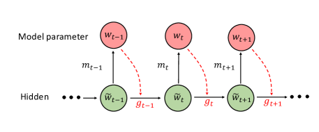
Figure 1: OPT-AMSGrad underlying structure.

In the following analysis, we show that this interleaving actually leads to some cancellation in the regret bound. Such two-levels method where the guess $m_{t}$ is equal to the last known gradient $g_{t-1}$ has been exhibited recently in [8]. The gradient prediction process plays an important role as discussed in Section 6. The proposed OPT-AMSGrad algorithm inherits three properties: (i) Adaptive learning rate of each dimension as AdaGrad [12] (line 6, line 8 and line 9). (ii) Exponential moving average of the past gradients as Nesterov’s method [29] and the Heavy-Ball method [30] (line 5). (iii) Optimistic update that exploits prior knowledge of the next gradient vector as in optimistic online learning algorithms [8, 31, 35] (line 9). The first property helps for acceleration when the gradient has a sparse structure. The second one is from the long-established idea of momentum which can also help for acceleration. The last property can lead to an acceleration when the prediction of the next gradient is good as mentioned above when introducing the regret bound for the Optimistic-FTRL algorithm. This property will be elaborated whilst establishing the theoretical analysis of OPT-AMSGrad.

4 Convergence Analysis

In this section, we provide regret analysis of the proposed method and show that it can improve the bound of vanilla AMSGrad with a good guess of the gradient. The convex result is followed by a global non-asymptotic analysis for nonconvex objective functions where the optimization problem tackled in this paper is cast as an offline and stochastic nonconvex optimization problem.

More notations.    We denote the Mahalanobis norm by $\|\cdot\|_{H}:=\sqrt{\langle\cdot,H\cdot\rangle}$ for some positive semidefinite (PSD) matrix $H$. We let $\psi_{t}(x):=\langle x,\text{diag}\{\hat{v}_{t}\}^{1/2}x\rangle$ for a PSD matrix $H_{t}^{1/2}:=\text{diag}\{\hat{v}_{t}\}^{1/2}$, where $\text{diag}\{\hat{v}_{t}\}$ represents the diagonal matrix which $i_{th}$ diagonal element is $\hat{v}_{t}[i]$ defined in Algorithm 2. We define its corresponding Mahalanobis norm by $\|\cdot\|_{\psi_{t}}:=\sqrt{\langle\cdot,\text{diag}\{\hat{v}_{t}\}^{1/2}\cdot\rangle}$, where we abuse the notation $\psi_{t}$ to represent the PSD matrix $H_{t}^{1/2}:=\text{diag}\{\hat{v}_{t}\}^{1/2}$. Note that $\psi_{t}(\cdot)$ is 1-strongly convex with respect to the norm $\|\cdot\|_{\psi_{t}}$, i.e., $\psi_{t}(\cdot)$ satisfies $\psi_{t}(u)\geq\psi_{t}(v)+\langle\psi_{t}(v),u-v\rangle+\frac{1}{2}\|u-v\|^{2}_{\psi_{t}}$ for any point $(u,v)\in\Theta^{2}$. A consequence of 1-strong convexity of $\psi_{t}(\cdot)$ is that $B_{\psi_{t}}(u,v)\geq\frac{1}{2}\|u-v\|^{2}_{\psi_{t}}$, where the Bregman divergence $B_{\psi_{t}}(u,v)$ is defined as $B_{\psi_{t}}(u,v):=\psi_{t}(u)-\psi_{t}(v)-\langle\psi_{t}(v),u-v\rangle$ with $\psi_{t}(\cdot)$ as the distance generating function. We also define the corresponding dual norm $\|\cdot\|_{\psi_{t}^{*}}:=\sqrt{\langle\cdot,\text{diag}\{\hat{v}_{t}\}^{-1/2}\cdot\rangle}$. The proofs of the following theoretical results are deferred to the Appendix.

4.1 Convex Regret Analysis

In the following, we assume convexity of $\{\ell_{t}\}_{t>0}$ and that $\Theta$ has a bounded diameter $D_{\infty}$, which is a standard assumption for adaptive methods [32, 20] and is necessary in regret analysis.

Theorem 1.

Suppose the learner incurs a sequence of convex loss functions $\{\ell_{t}(\cdot)\}$. Then, OPT-AMSGrad (Algorithm 2) has regret

$$\begin{split}\mathcal{R}_{T}\leq\frac{B_{\psi_{1}}(w^{*},\tilde{w}_{1})}{\eta_{1}}+\sum_{t=1}^{T}\frac{\eta_{t}}{2}\|g_{t}-\tilde{m}_{t}\|_{\psi_{t-1}^{*}}^{2}+\frac{D_{\infty}^{2}}{\eta_{\min}}\sum_{i=1}^{d}\hat{v}_{T}^{1/2}[i]+D_{\infty}^{2}\beta_{1}^{2}\sum_{t=1}^{T}\|g_{t}-\theta_{t-1}\|_{\psi_{t-1}^{*}}\;,\end{split}$$

where $\tilde{m}_{t+1}=\beta_{1}\theta_{t-1}+(1-\beta_{1})m_{t+1}$, $g_{t}:=\nabla\ell_{t}(w_{t})$, $\eta_{{\min}}:=\min_{{t}}\eta_{t}$ and $D_{\infty}^{2}$ is the diameter of the bounded set $\Theta$. The result holds for any benchmark $w^{*}\in\Theta$ and any step size sequence $\{\eta_{t}\}_{t>0}$.

Corollary 1.

Suppose $\beta_{1}=0$ and $\{v_{t}\}_{t>0}$ is a monotonically increasing sequence, then we obtain the following regret bound for any $w^{*}\in\Theta$ and sequence of stepsizes $\{\eta_{t}=\eta/\sqrt{t}\}_{t>0}$:

$$\begin{split}\mathcal{R}_{T}\leq\frac{B_{\psi_{1}}}{\eta_{1}}+\frac{\eta\sqrt{1+\log T}}{\sqrt{1-\beta_{2}}}\sum_{i=1}^{d}\|(g-m)_{1:T}[i]\|_{2}+\frac{D_{\infty}^{2}}{\eta_{\min}}\sum_{i=1}^{d}\left[(1-\beta_{2})\sum_{s=1}^{T}\beta_{2}^{T-s}g^{2}_{s}[i]\right]^{1/2}\;,\end{split}$$

where $B_{\psi_{1}}:=B_{\psi_{1}}(w^{*},\tilde{w}_{1})$, $g_{t}:=\nabla\ell_{t}(w_{t})$ and $\eta_{{\min}}:=\min_{{t}}\eta_{t}$.

We can compare the bound of Corollary 1 with that of AMSGrad [32] with $\eta_{t}=\eta/\sqrt{t}$:

$$\mathcal{R}_{T}\leq\frac{\eta\sqrt{1+\log T}}{\sqrt{1-\beta_{2}}}\sum_{i=1}^{d}\|g_{1:T}[i]\|_{2}+\frac{\sqrt{T}}{2\eta}D^{2}_{\infty}\sum_{i=1}^{d}\hat{v}_{T}[i]^{2}\;.$$ (1)

For convex regret minimization, Corollary 1 yields a regret of $\mathcal{O}(\sqrt{\sum_{t=1}^{T}\|g_{t}-m_{t}\|^{2}_{\psi^{*}_{t-1}}})$ with an access to an arbitrary predictable process $\{m_{t}\}_{t>0}$ of the mini-batch gradients. We notice from the second term in Corollary 1 compared to the first term in (1) that better predictors lead to lower regret. The construction of the predictions $\{m_{t}\}_{t>0}$ is thus of utmost importance for achieving optimal acceleration and can be learned through the iterations [31]. In Section 6, we derive a basic, yet effective, gradient prediction algorithm, see Algorithm 4, embedded in OPT-AMSGrad.

4.2 Finite-Time Analysis in Nonconvex Case

We discuss the offline and stochastic nonconvex optimization properties of our online framework. As stated in the introduction, this paper is about solving optimization problems instead of solving zero-sum games. Classically, the optimization problem we are tackling reads:

$$\min\limits_{w\in\Theta}f(w)\mathrel{\mathop{:}}=\mathbb{E}[f(w,\xi)]=n^{-1}\sum_{i=1}^{n}\mathbb{E}[f(w,\xi_{i})]\;,$$ (2)

for a fixed batch of $n$ samples $\{\xi_{i}\}_{i=1}^{n}$. The objective function $f(\cdot)$ is (potentially) nonconvex and has Lipschitz gradients. Set the terminating number, $T\in\{0,\dots,T_{\sf M}-1\}$, as a discrete r.v. with:

$$P(T=\ell)=\frac{\eta_{\ell}}{\sum_{j=0}^{T_{\sf M}-1}\eta_{j}}\;,$$ (3)

where $T_{\sf M}$ is the maximum number of iteration. The random termination number (3) is inspired by [15] and is widely used to derive novel results in nonconvex optimization. Consider the following assumptions:

H​​ 1.

For any $t>0$, the estimated parameter $w_{t}$ stays within a $\ell_{\infty}-$ball. There exists a constant $W>0$ such that $\left\|w_{t}\right\|_{\infty}\leq W$ almost surely.

H​​ 2.

The function $f$ is $L$-smooth (has $L$-Lipschitz gradients) w.r.t. the parameter w. There exist some constant $L>0$ such that for $(w,\vartheta)\in\Theta^{2}$, $f(w)-f(\vartheta)-\nabla f(\vartheta)^{\top}(w-\vartheta)\leq\frac{L}{2}\left\|w-\vartheta\right\|^{2}\;.$

For nonconvex analysis, we assume the following:

H​​ 3.

For any $t>0$, $0<\left\langle m_{t}\,|\,g_{t}\right\rangle=a_{t}\|g_{t}\|^{2}$ with some $0<a_{t}\leq 1$, and $\|m_{t}\|\leq\|g_{t}\|$, where $\left\langle\,|\,\right\rangle$ denotes the inner product.

H3 assumes that the predicted gradient is in general reasonable, in the sense that $m_{t}$ has acute angle with $g_{t}$ and bounded norm, as the shadowed area in Figure 2.

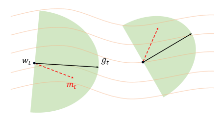
Figure 2: Illustration of H3.

Lastly, We make a classical assumption in nonconvex optimization on the magnitude of the gradient:

H​​ 4.

There exists a constant $\mathsf{M}>0$ such that for any $w$ and $\xi$, it holds that $\left\|\nabla f(w,\xi)\right\|<\mathsf{M}$.

We now derive important results for our global analysis. The first one ensures bounded norms of quantities of interests (resulting from the bounded stochastic gradient assumption):

Lemma 1.

Assume H4, then the quantities defined in Algorithm 2 satisfy for any $w\in\Theta$ and $t>0$, $\|\nabla f(w_{t})\|<\mathsf{M},~{}~{}~{}\|\theta_{t}\|<\mathsf{M}$ and $\|\hat{v}_{t}\|<\mathsf{M}^{2}$.

We now formulate the main result of our paper yielding a finite-time upper bound of the suboptimality condition defined as $\mathbb{E}\left[\|\nabla f(w_{T})\|^{2}\right]$ (set as the convergence criterion of interest, see [15]):

Theorem 2.

Assume H1-H4, $\beta_{1}<\beta_{2}\in[0,1)$ and a sequence of decreasing stepsizes $\{\eta_{t}\}_{t>0}$, then the following result holds:

$$\begin{split}\mathbb{E}\left[\|\nabla f(w_{T})\|_{2}^{2}\right]\leq\tilde{C}_{1}\sqrt{\frac{d}{T_{\sf M}}}+\tilde{C}_{2}\frac{1}{T_{\sf M}}\;,\end{split}$$

where $T$ is a random termination number distributed according (3). The constants are defined as:

$$\tilde{C}_{1}=\frac{\mathsf{M}}{(1-a_{m}\beta_{1})+(\beta_{1}+a_{m})}\left[\frac{a_{m}(1-\beta_{1})^{2}}{1-\beta_{2}}+2L\frac{1}{1-\beta_{2}}+\Delta f+\frac{4L\beta_{1}^{2}(1+\beta_{1}^{2})}{(1-\beta_{1})(1-\beta_{2})(1-\gamma)}\right],$$

$$\tilde{C}_{2}=\frac{\mathsf{M}^{2}}{(1-\beta_{1})\left((1-a_{m}\beta_{1})+(\beta_{1}+a_{m})\right)}\left[a_{m}\beta_{1}^{2}-2a_{m}\beta_{1}+\beta_{1}\right]\mathbb{E}\left[\left\|\hat{v}_{0}^{-1/2}\right\|\right]\;,$$

where $\Delta f=f(\overline{w}_{1})-f(\overline{w}_{T_{\sf M}+1})$ and $a_{m}=\displaystyle{\min_{t=1,...,T}}a_{t}$.

Firstly, the bound for our OPT-AMSGrad method matches the complexity bound of $\mathcal{O}(\sqrt{d/T_{\sf M}}+1/T_{\sf M})$ of [15] for SGD considering the dependence of T only, and of [43] for AMSGrad method.To see the influence of prediction quality, we can show that when $(1-\beta_{1})(\beta_{2}-\beta_{1}^{2}-2L(1-\beta_{1}))-\frac{4L\beta_{1}^{2}(1+\beta_{1}^{2})}{1-\gamma}<0$, $\tilde{C}_{1}$ and $\tilde{C}_{2}$ both decrease as $a_{m}$ approaches 1, i.e., as the prediction gets more accurate. Therefore, similar to the convex case, our nonconvex bound also improves with better gradient prediction.

4.3 Checking H1 for a Deep Neural Network

As boundedness assumption H1 is generally hard to verify, we now show, for illustrative purposes, that the weights of a fully connected feed forward neural network stay in a bounded set when being trained using our method. The activation function for this section will be sigmoid function and we use a $\ell_{2}$ regularization. We consider a fully connected feed forward neural network with $L$ layers modeled by the function $\textsf{MLN}(w,\xi):\Theta^{d}\times\mathbb{R}^{p}\to\mathbb{R}$ defined as:

$$\textsf{MLN}(w,\xi)=\sigma\left(w^{(L)}\sigma\left(w^{(L-1)}\ldots\sigma\left(w^{(1)}\xi\right)\right)\right)\;,$$ (4)

where $w=[w^{(1)},w^{(2)},\cdots,w^{(L)}]$ is the vector of parameters, $\xi\in\mathbb{R}^{p}$ is the input data and $\sigma$ is the sigmoid activation function. We assume a $p$ dimension input data and a scalar output for simplicity. In this setting, the stochastic objective function (2) reads

$$f(w,\xi)=\mathcal{L}(\textsf{MLN}(w,\xi),y)+\frac{\lambda}{2}\left\|w\right\|^{2}\;,$$

where $\mathcal{L}(\cdot,y)$ is the loss function (e.g., cross-entropy), $y$ are the true labels and $\lambda>0$ is the regularization parameter. We establish that the boundedness assumption H1 is satisfied with model (4) via the following:

Lemma 2.

Given the multilayer model (4), assume the boundedness of the input data and of the loss function, i.e., for any $\xi\in\mathbb{R}^{p}$ and $y\in\mathbb{R}$ there is a constant $T>0$ such that $\left\|\xi\right\|\leq 1\quad\textrm{a.s.}$ and $|\mathcal{L}^{\prime}(\cdot,y)|\leq T$ where $\mathcal{L}^{\prime}(\cdot,y)$ denotes its derivative w.r.t. the parameter. Then for each layer $\ell\in[1,L]$, there exists a constant $A_{(\ell)}$ such that $\left\|w^{(\ell)}\right\|\leq A_{(\ell)}$.

5 Comparison to related methods

We give in this section some comparable methods to our OPT-AMSGrad algorithm such as AO-FTRL [28] or Optimistic-Adam [9].

Comparison to nonconvex optimization works.    Recently, [41, 6, 39, 43, 45, 24] provide some theoretical analysis of Adam-type algorithms when applying them to smooth nonconvex optimization problems. For example, [6] provide the following bound $\min_{t\in[T]}\mathbb{E}[\|\nabla f(w_{t})\|^{2}]=\mathcal{O}(\log T/\sqrt{T})$. Yet, this data independent bound does not show any advantage over standard stochastic gradient descent. Similar concerns appear in other related works. To get some adaptive data dependent bound written in terms of the gradient norms observed along the trajectory when applying OPT-AMSGrad to nonconvex optimization, one can follow the approach of [2] or [7]. They provide a modular approach to convert algorithms with adaptive data dependent regret bound for convex loss functions (e.g., AdaGrad) to algorithms that can find an approximate stationary point of nonconvex objectives. These variants can outperform the ones instantiated by other Adam-type algorithms when the gradient prediction $m_{t}$ is close to the true gradient $g_{t}$.

Comparison to AO-FTRL [28].   In [28], the authors propose AO-FTRL, which update reads $w_{t+1}=\arg\min_{{w\in\Theta}}(\sum_{s=1}^{t}g_{s})^{\top}w+m_{t+1}^{\top}w+r_{0:t}(w)$, where $r_{0:t}(\cdot)$ is a 1-strongly convex loss function with respect to some norm $\|\cdot\|_{(t)}$ that may be different for different iteration $t$. Data dependent regret bound provided in [28] reads $r_{{0:T}}(w^{*})+\sum_{t=1}^{T}\|g_{t}-m_{t}\|_{(t)^{*}}$ for any benchmark $w^{*}\in\Theta$. We remark that if one selects $r_{0:t}(w):=\langle w,\text{diag}\{\hat{v}_{t}\}^{1/2}w\rangle$ and $\|\cdot\|_{(t)}:=\sqrt{\langle\cdot,\text{diag}\{\hat{v}_{t}\}^{1/2}\cdot\rangle}$, then the update might be viewed as an optimistic variant of AdaGrad. However, no experiments were provided in [28] to back those findings.

Comparison to Optimistic-Adam [9]. This is an optimistic variant of ADAM, namely Optimistic-Adam. A slightly modified version is summarized in Algorithm 3. Here, Optimistic-Adam$+\hat{v}_{t}$ corresponds to Optimistic-Adam with the additional max operation $\hat{v}_{t}=\max(\hat{v}_{t-1},v_{t})$ to guarantee that the weighted second moment is monotone increasing. We want to emphasize that the motivations of our optimistic algorithm are different. Optimistic-Adam is designed to optimize two-player games (e.g., GANs [16]), while our proposed algorithm OPT-AMSGrad is designed to accelerate optimization (e.g., solving empirical risk minimization). [9] focuses on training GANs [16] as a two-player zero-sum game. [9] was inspired by these related works and showed that Optimistic-Mirror-Descent can avoid the cycle behavior in a bilinear zero-sum game, which accelerates the convergence.

1:  Required: parameter $\beta_{1}$, $\beta_{2}$, and $\eta_{t}$.

2:  Init: $w_{1}\in\Theta$ and $\hat{v}_{0}=v_{0}=\epsilon 1\in\mathbb{R}^{d}$.

3:  for $t=1$ to $T$ do

4:     Compute stochastic gradient vector $g_{t}$ at $w_{t}$.

5:     $\theta_{t}=\beta_{1}\theta_{t-1}+(1-\beta_{1})g_{t}$.

6:     $v_{t}=\beta_{2}v_{t-1}+(1-\beta_{2})g_{t}^{2}$.

7:     $\hat{v}_{t}=\max(\hat{v}_{t-1},v_{t})$.

8:     $w_{t+1}=\Pi_{k}[w_{t}-2\eta_{t}\frac{\theta_{t}}{\sqrt{\hat{v}_{t}}}+\eta_{t}\frac{\theta_{t-1}}{\sqrt{\hat{v}_{t-1}}}]$.

9:  end for

Algorithm 3 Optimistic-Adam [9]+$\hat{v}_{t}$.

6 Numerical Experiments

In this section, we provide experiments on classification tasks with various neural network architectures and datasets to demonstrate the effectiveness of OPT-AMSGrad in practice and justify its theoretical convergence acceleration. We start with giving an overview of the gradient predictor process before presenting our numerical runs.

6.1 Gradient Estimation

Based on the analysis in the previous section, we understand that the choice of the prediction $m_{t}$ plays an important role in the convergence of Optimistic-AMSGrad. Some classical works in gradient prediction methods include Anderson acceleration [38], Minimal Polynomial Extrapolation [4] and Reduced Rank Extrapolation [13]. These methods typically assume that the sequence $\{g_{t}\}\in\mathbb{R}^{d}$ has a linear relation $g_{t}=A(g_{t-1}-g^{*})+g^{*}$ where $A\in\mathbb{R}^{d\times d}$ is an unknown, not necessarily symmetric, matrix. Then, these methods aim at finding a fixed point $g^{*}$ and assume that $\{g_{t}\in\mathbb{R}^{d}\}_{t>0}$ has the following linear relation:

$$g_{t}-g^{*}=A(g_{t-1}-g^{*})+e_{t},$$ (5)

where $e_{t}$ is a second order term satisfying $\|e_{t}\|_{2}=\mathcal{O}(\|g_{t-1}-g^{*}\|_{2}^{2})$, see [33] for details and results. For our numerical experiments, we run OPT-AMSGrad using Algorithm 4 to construct the sequence $\{m_{t}\}_{t>0}$ which is based on estimating the limit of a sequence using the last iterates [3].

1:  Input: sequence $\{g_{s}\in\mathbb{R}^{d}\}_{s=0}^{s=r-1}$, parameter $\lambda>0$.

2:  Compute matrix $U=[g_{1}-g_{0},\dots,g_{r}-g_{r-1}]\in\mathbb{R}^{d\times r}$.

3:  Obtain $z$ by solving $(U^{\top}U+\lambda I)z=\mathbf{1}$.

4:  Get $c=z/(z^{\top}\mathbf{1})$.

5:  Output: $\Sigma_{i=0}^{r-1}c_{i}g_{i}$, the approximation of the fixed point $g^{*}$.

Algorithm 4 Regularized Approximated Minimal Polynomial Extrapolation [33]

Specifically, at iteration $t$, $m_{t}$ is obtained by (a) calling Algorithm 4 with a sequence of $r$ past gradients, $\{g_{t-1},g_{t-2},\dots,g_{t-r}\}$ as input yielding the vector $c=[c_{0},\dots,c_{r-1}]$ and (b) setting $m_{t}:=\Sigma_{i=0}^{r-1}c_{i}g_{t-r+i}$. To understand why the output from the extrapolation method may be a reasonable estimation, assume that the update converges to a stationary point (i.e., $g^{*}:=\nabla f(w^{*})=0$ for the underlying function $f$). Then, we might rewrite (5) as $g_{t}=Ag_{t-1}+\mathcal{O}(\|g_{t-1}\|_{2}^{2})u_{t-1}$, for some unit vector $u_{t-1}$. This equation suggests that the next gradient vector $g_{t}$ is a linear transform of $g_{{t-1}}$ plus an error vector that may not be in the span of $A$. If the algorithm converges to a stationary point, the magnitude of the error will converge to zero. We note that prior known gradient prediction methods are mainly designed for convex functions. Algorithm 4 is used in our following numerical applications given its empirical success in Deep Learning, see [34], yet, any gradient prediction method can be embedded in our OPT-AMSGrad framework. The search for the optimal prediction process in order to accelerate OPT-AMSGrad is an interesting research direction.

Computational cost: This extrapolation step consists in: (a) Constructing the linear system $(U^{\top}U)$ which cost can be optimized to $\mathcal{O}(d)$, since the matrix $U$ only changes one column at a time. (b) Solving the linear system which cost is $\mathcal{O}(r^{3})$, and is negligible for a small $r$ used in practice. (c) Outputting a weighted average of previous gradients which cost is $\mathcal{O}(r\times d)$ yielding a computational overhead of $\mathcal{O}\left((r+1)d+r^{3}\right)$. Yet, steps (a) and (c) are parallelizable in the final implementation.

6.2 Classification Experiments

Methods. We consider two baselines. The first one is the original AMSGrad. The hyper-parameters are set to be $\beta_{1}=0.9$ and $\beta_{2}=0.999$, see [32]. The other benchmark method is the Optimistic-Adam$+\hat{v}_{t}$ [9], which described Algorithm 3. We use cross-entropy loss, a mini-batch size of $128$ and tune the learning rates over a fine grid and report the best result for all methods. For OPT-AMSGrad, we use $\beta_{1}=0.9$ and $\beta_{2}=0.999$ and the best step size $\eta$ of AMSGrad for a fair evaluation of the optimistic step. In our implementation, OPT-AMSGrad has an additional parameter $r$ that controls the number of previous gradients used for gradient prediction. We use $r=5$ past gradient for empirical reasons, see Section 6.3. The algorithms are initialized at the same point and the results are averaged over 5 repetitions.

Datasets.   Following [32, 20], we compare different algorithms on MNIST, CIFAR10, CIFAR100, and IMDB datasets. For MNIST, we use two noisy variants namely MNIST-back-rand and MNIST-back-image from [21] (which was also heavily used in [23] to evaluate tree algorithms). They both have $12\,000$ training samples and $50\,000$ test samples, where random background is inserted to the original MNIST hand-written digit images. For MNIST-back-rand, each image is inserted with a random background, which pixel values are generated uniformly from 0 to 255, while MNIST-back-image takes random patches from a black and white noisy background. The input dimension is $784$ ($28\times 28$) and the number of classes is $10$. CIFAR10 and CIFAR100 are popular computer-vision datasets of $50\,000$ training images and $10\,000$ test images, of size $32\times 32$. The IMDB movie review dataset is a binary classification dataset with $25\,000$ training and testing samples respectively. It is a popular dataset for text classification.

Network architectures. We adopt a multi-layer fully connected neural network with hidden layers of $200$ connected to another layer with $100$ neurons (using ReLU activations and Softmax output). This network is tested on MNIST variants. For convolutional networks, we adopt a simple four layer CNN which has 2 convolutional layers following by a fully connected layer. In addition, we also apply residual networks, Resnet-18 and Resnet-50 [19], which have achieved state-of-the-art results. For the texture IMDB dataset, we consider a Long-Short Term Memory (LSTM) network [14]. The latter network includes a word embedding layer with $5\,000$ input entries representing most frequent words embedded into a $32$ dimensional space. The output of the embedding layer is passed to $100$ LSTM units then connected to $100$ fully connected ReLU layers.

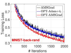
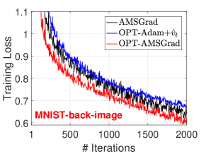
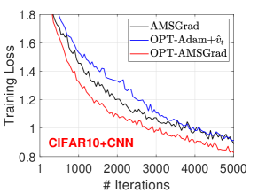
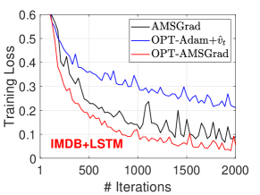
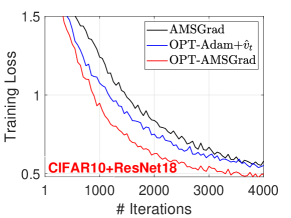
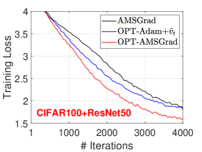
Figure 3: Training loss vs. number of iterations for fully connected NN, CNN, LSTM and ResNet.

Results. Firstly, to illustrate the acceleration effect of OPT-AMSGrad at early stage, we provide the training loss against number of iterations in Figure 3. Clearly, on all datasets, the proposed OPT-AMSGrad converges faster than the other competing methods since fewer iterations are required to achieve the same precision, validating one of the main edges of OPT-AMSGrad. We are also curious about the long-term performance and generalization of the proposed method in test phase. In Figure 4, we plot the results when the model is trained until the test accuracy stabilizes. We observe: (1) in the long term, OPT-AMSGrad algorithm may converge to a better point with smaller objective function value, and (2) in these three applications, OPT-AMSGrad also outperforms the competing methods in terms of test accuracy.

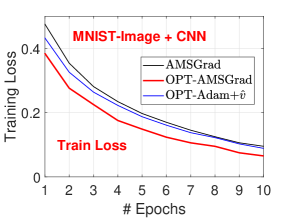
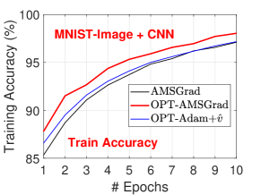
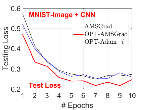
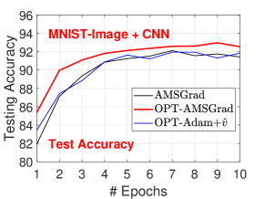
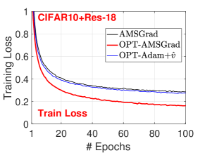
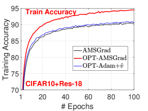
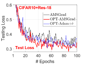
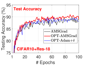
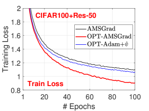
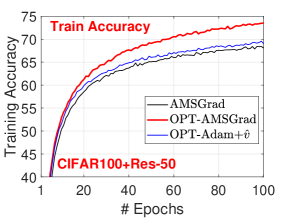
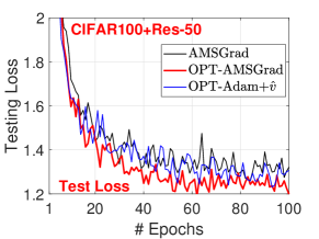
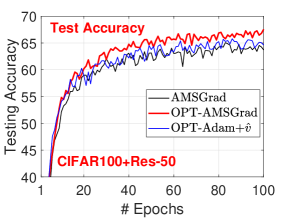
Figure 4: MNIST-back-image + CNN, CIFAR10 + Res-18 and CIFAR100 + Res-50 . We compare three methods in terms of training (cross-entropy) loss and accuracy, testing loss and accuracy.

6.3 Choice of parameter $r$

Since the number of past gradients $r$ is important in gradient prediction (Algorithm 4), we compare Figure 5 the performance under different values $r=3,5,10$ on two datasets. From the results we see that, taking into consideration both quality of gradient prediction and computational cost, $r=5$ is a good choice for most applications. We remark that, empirically, the performance comparison among $r=3,5,10$ is not absolutely consistent (i.e., more means better) in all cases. We suspect one possible reason is that for deep neural networks, the diversity of computed gradients through the iterations, due to the highly nonconvex loss, makes them inefficient for sequentially building the predictable process $\{m_{t}\}_{t>0}$. Thus, sometimes, the recent gradient vectors (e.g., $r\leq 5$) can be more informative. Yet, in some sense, this characteristic, very specific to deep neural networks, is itself a fundamental problem of gradient prediction methods.

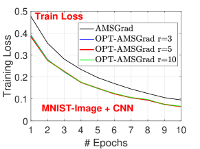
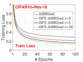
Figure 5: Training loss w.r.t. different $r$ values.

7 Conclusion

In this paper, we propose OPT-AMSGrad, which combines optimistic online learning and AMSGrad to improve sample efficiency and accelerate the training process, in particular for deep neural networks. Given a good gradient prediction process, we demonstrate that the regret can be smaller than that of standard AMSGrad. We also establish finite-time convergence bound on the second order moment of the gradient of the objective function matching that of state-of-the-art algorithms. Experiments on various deep learning problems demonstrate the effectiveness of the proposed algorithm in accelerating the empirical risk minimization procedure and empirically show better generalization properties of OPT-AMSGrad.

Appendix A Additional Remarks on the Gradient Prediction Process

Two illustrative examples.    We provide two toy examples to demonstrate how OPT-AMSGrad works with the chosen extrapolation method. First, consider minimizing a quadratic function $H(w):=\frac{b}{2}w^{2}$ with vanilla gradient descent method $w_{t+1}=w_{t}-\eta_{t}\nabla H(w_{t})$. The gradient $g_{t}:=\nabla H(w_{t})$ can be recursively expressed as $g_{t+1}=bw_{t+1}=b(w_{t}-\eta_{t}g_{t})=g_{t}-b\eta_{t}g_{t}$. Thus, the update can be written in the form of

$$g_{t}=Ag_{t-1}+\mathcal{O}(\|g_{t-1}\|_{2}^{2})u_{t-1}\,,$$

where $A=(1-b\eta)$ and $u_{t-1}=0$ by setting $\eta_{t}=\eta$ (constant step size). Specifically, consider optimizing $H(w):=w^{2}/2$ by the following three algorithms with the same step size. One is Gradient Descent (GD): $w_{t+1}=w_{t}-\eta_{t}g_{t}$, while the other two are OPT-AMSGrad with $\beta_{1}=0$ and the second moment term $\hat{v}_{t}$ being dropped: $w_{t+\frac{1}{2}}=\Pi_{\Theta}\big{[}w_{t-\frac{1}{2}}-\eta_{t}g_{t}\big{]}$, $w_{t+1}=\Pi_{\Theta}\big{[}w_{t+\frac{1}{2}}-\eta_{t+1}m_{t+1}\big{]}$. We denote the algorithm that sets $m_{t+1}=g_{t}$ as Opt-1, and denote the algorithm that uses the extrapolation method to get $m_{t+1}$ as Opt-extra. We let $\eta_{t}=0.1$ and the initial point $w_{0}=5$ for all three methods.

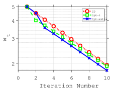
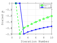
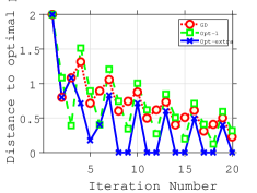
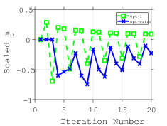
Figure 6: (a): The iterate $w_{t}$; the closer to the optimal point $0$ the better. (b): A scaled and clipped version of $m_{t}$: $w_{t}-w_{t-1/2}$, which measures how the prediction of $m_{t}$ drives the update towards the optimal point. In this scenario, the more negative the better. (c): Distance to the optimal point $-1$. The smaller the better. (d): A scaled and clipped version of $m_{t}$: $w_{t}-w_{t-1/2}$, which measures how the prediction of $m_{t}$ drives the update towards the optimal point. In this scenario, the more negative the better.

The simulation results are on Figure 6 (a) and (b). Sub-figure (a) plots the updates $\{w_{t}\}_{t>0}$ through the iterations, where the updates go towards the optimal point $0$. Sub-figure (b) displays a scaled and clipped version of $m_{t}$, defined as $w_{t}-w_{t-1/2}$, which can be viewed as $-\eta_{t}m_{t}$ if the projection (if existing) is lifted. Sub-figure (a) shows that Opt-extra converges faster than the other methods. Furthermore, sub-figure (b) shows that the prediction by the extrapolation method is better than the prediction by simply using the previous gradient. The sub-figure shows that $-m_{t}$ from both methods points to $0$ for each iteration and the magnitude is larger for the one produced by the extrapolation method after iteration $2$.

Now let us consider another problem: an online learning problem proposed in [32] . Assume the learner’s decision space is $\Theta=[-1,1]$, and the loss function is $\ell_{t}(w)=3w$ if $t\text{ mod }3=1$, and $\ell_{t}(w)=-w$ otherwise. The optimal point to minimize the cumulative loss is $w^{*}=-1$. We let $\eta_{t}=0.1/\sqrt{t}$ and the initial point $w_{0}=1$ for all three methods. The parameter $\lambda$ of the extrapolation method is set to $\lambda=10^{-3}>0$. The results are reported Figure 6 (c) and (d). Sub-figure (c) shows that Opt-extra converges faster than the other methods while Opt-1 is not performing better than GD. The reason is that the gradient changes from $-1$ to $3$ at $t\text{ mod }3=1$ and it changes from $3$ to $-1$ at $t\text{ mod }3=2$. Consequently, using the current gradient as the guess for the next is empirically not a good choice, since the next gradient is in the opposite direction of the current one, according to our experiments. Sub-figure (d) shows that $-m_{t}$, obtained with the extrapolation method, always points to $w^{*}=-1$, while the one obtained by using the previous negative direction points to the opposite direction in two thirds of rounds. It empirically shows that the extrapolation method is much less affected by the gradient oscillation and always makes the prediction in the right direction, which suggests that the method can capture the aggregate effect.

Appendix B Proof of Theorem 1

Theorem.

Suppose the learner incurs a sequence of convex loss functions $\{\ell_{t}(\cdot)\}$. Then, OPT-AMSGrad (Algorithm 2) has regret

$$\mathcal{R}_{T}\leq \frac{B_{\psi_{1}}(w^{*},\tilde{w}_{1})}{\eta_{1}}+\sum_{t=1}^{T}\frac{\eta_{t}}{2}\|g_{t}-\tilde{m}_{t}\|_{\psi_{t-1}^{*}}^{2}+\frac{D_{\infty}^{2}}{\eta_{\min}}\sum_{i=1}^{d}\hat{v}_{T}^{1/2}[i]+D_{\infty}^{2}\beta_{1}^{2}\sum_{t=1}^{T}\|g_{t}-\theta_{t-1}\|_{\psi_{t-1}^{*}}\;,$$

where $\tilde{m}_{t+1}=\beta_{1}\theta_{t-1}+(1-\beta_{1})m_{t+1}$, $g_{t}:=\nabla\ell_{t}(w_{t})$, $\eta_{{\min}}:=\min_{{t}}\eta_{t}$ and $D_{\infty}^{2}$ is the diameter of the bounded set $\Theta$. The result holds for any benchmark $w^{*}\in\Theta$ and any step size sequence $\{\eta_{t}\}_{t>0}$.

Proof.

Beforehand, we denote:

$$\begin{split}&\tilde{g}_{t}=\beta_{1}\theta_{t-1}+(1-\beta_{1})g_{t}\,,\\ &\tilde{m}_{t+1}=\beta_{1}\theta_{t-1}+(1-\beta_{1})m_{t+1}\,,\end{split}$$

where we recall that $g_{t}$ and $m_{t+1}$ are respectively the gradient $\nabla\ell_{t}(w_{t})$ and the predictable guess. By regret decomposition, we have that

$$\mathcal{R}_{T}:=\sum_{t=1}^{T}\ell_{t}(w_{t})-\min_{w\in\Theta}\sum_{t=1}^{T}\ell_{t}(w)\textstyle$$ (6)

$$\leq \sum_{t=1}^{T}\langle w_{t}-w^{*},\nabla\ell_{t}(w_{t})\rangle$$

$$= \sum_{t=1}^{T}\langle w_{t}-\tilde{w}_{t+1},g_{t}-\tilde{m}_{t}\rangle+\langle w_{t}-\tilde{w}_{t+1},\tilde{m}_{t}\rangle+\langle\tilde{w}_{t+1}-w^{*},\tilde{g}_{t}\rangle+\langle\tilde{w}_{t+1}-w^{*},g_{t}-\tilde{g}_{t}\rangle\;.$$

Recall the notation $\psi_{t}(x)$ and the Bregman divergence $B_{\psi_{t}}(u,v)$ defined Section 4. We exploit a useful inequality (which appears in e.g., [37]). For any update of the form $\hat{w}=\arg\min_{w\in\Theta}\langle w,\theta\rangle+B_{\psi}(w,v)$, it holds that

$$\langle\hat{w}-u,\theta\rangle\leq B_{\psi}(u,v)-B_{\psi}(u,\hat{w})-B_{\psi}(\hat{w},v)\quad\textrm{for any $u\in\Theta$}\;.$$ (7)

For $\beta_{1}=0$, we can rewrite the update on line 8 of (Algorithm 2) as

$$\tilde{w}_{t+1}=\arg\min_{w\in\Theta}\eta_{t}\langle w,\tilde{g}_{t}\rangle+B_{\psi_{t}}(w,\tilde{w}_{t})\;.$$ (8)

By using (7) for (8) with $\hat{w}=\tilde{w}_{t+1}$ (the output of the minimization problem), $u=w^{*}$ and $v=\tilde{w}_{t}$, we have

$$\langle\tilde{w}_{t+1}-w^{*}, \tilde{g}_{t}\rangle\leq\frac{1}{\eta_{t}}\big{[}B_{\psi_{t}}(w^{*},\tilde{w}_{t})-B_{\psi_{t}}(w^{*},\tilde{w}_{t+1})-B_{\psi_{t}}(\tilde{w}_{t+1},\tilde{w}_{t})\big{]}\;.$$ (9)

We can also rewrite the update on line 9 of (Algorithm 2) at time $t$ as

$$\textstyle w_{t+1}=\arg\min_{w\in\Theta}\eta_{t+1}\langle w,\tilde{m}_{t+1}\rangle+B_{\psi_{t}}(w,\tilde{w}_{t+1})\;.$$ (10)

and, by using (7) for (10) (written at iteration $t$), with $\hat{w}=w_{t}$ (the output of the minimization problem), $u=\tilde{w}_{t+1}$ and $v=\tilde{w}_{t}$, we have

$$\langle w_{t}-\tilde{w}_{t+1}, \tilde{m}_{t}\rangle\leq\frac{1}{\eta_{t}}\big{[}B_{\psi_{t-1}}(\tilde{w}_{t+1},\tilde{w}_{t})-B_{\psi_{t-1}}(\tilde{w}_{t+1},w_{t})-B_{\psi_{t-1}}(w_{t},\tilde{w}_{t})\big{]}\;.$$ (11)

By (6), (9), and (11), we obtain

$$\mathcal{R}_{T} \overset{(\ref{nn1})}{\leq}\sum_{t=1}^{T}\langle w_{t}-\tilde{w}_{t+1},g_{t}-\tilde{m}_{t}\rangle+\langle w_{t}-\tilde{w}_{t+1},\tilde{m}_{t}\rangle+\langle\tilde{w}_{t+1}-w^{*},\tilde{g}_{t}\rangle+\langle\tilde{w}_{t+1}-w^{*},g_{t}-\tilde{g}_{t}\rangle$$

$$\overset{(\ref{nn2}),(\ref{nn3})}{\leq}\sum_{t=1}^{T}\|w_{t}-\tilde{w}_{t+1}\|_{\psi_{t-1}}\|g_{t}-\tilde{m}_{t}\|_{\psi_{t-1}^{*}}+\|\tilde{w}_{t+1}-w^{*}\|_{\psi_{t-1}}\|g_{t}-\tilde{g}_{t}\|_{\psi_{t-1}^{*}}$$

$$+\frac{1}{\eta_{t}}\big{[}B_{\psi_{t-1}}(\tilde{w}_{t+1},\tilde{w}_{t})-B_{\psi_{t-1}}(\tilde{w}_{t+1},w_{t})-B_{\psi_{t-1}}(w_{t},\tilde{w}_{t})$$

$$+B_{\psi_{t}}(w^{*},\tilde{w}_{t})-B_{\psi_{t}}(w^{*},\tilde{w}_{t+1})-B_{\psi_{t}}(\tilde{w}_{t+1},\tilde{w}_{t})\big{]}\;,$$

which is further bounded by

$$\mathcal{R}_{T}\leq\sum_{t=1}^{T}\Big{\{} \frac{1}{2\eta_{t}}\|w_{t}-\tilde{w}_{t+1}\|_{\psi_{t-1}}^{2}+\frac{\eta_{t}}{2}\|g_{t}-m_{t}\|_{\psi_{t-1}^{*}}^{2}+\|\tilde{w}_{t+1}-w^{*}\|_{\psi_{t-1}}\|g_{t}-\tilde{g}_{t}\|_{\psi_{t-1}^{*}}$$ (12)

$$+\frac{1}{\eta_{t}}\big{(}\underbrace{B_{\psi_{t-1}}(\tilde{w}_{t+1},\tilde{w}_{t})-B_{\psi_{t}}(\tilde{w}_{t+1},\tilde{w}_{t})}_{A_{1}}-\frac{1}{2}\|\tilde{w}_{t+1}-w_{t}\|_{\psi_{t-1}}^{2}$$

$$+\underbrace{B_{\psi_{t}}(w^{*},\tilde{w}_{t})-B_{\psi_{t}}(w^{*},\tilde{w}_{t+1})}_{A_{2}}\big{)}\Big{\}}\;,$$

where the inequality is due to $\|w_{t}-\tilde{w}_{t+1}\|_{\psi_{t-1}}\|g_{t}-m_{t}\|_{\psi_{t-1}^{*}}=\inf_{\beta>0}\frac{1}{2\beta}\|w_{t}-\tilde{w}_{t+1}\|_{\psi_{t-1}}^{2}+\frac{\beta}{2}\|g_{t}-m_{t}\|_{\psi_{t-1}^{*}}^{2}$ by Young’s inequality and the 1-strongly convex of $\psi_{t-1}(\cdot)$ with respect to $\|\cdot\|_{\psi_{t-1}}$ which yields that $B_{\psi_{t-1}}(\tilde{w}_{t+1},w_{t})\geq\frac{1}{2}\|\tilde{w}_{t+1}-w_{t}\|^{2}_{\psi_{t}}\geq 0$.

To proceed, notice that

$$A_{1} :=B_{\psi_{t-1}}(\tilde{w}_{t+1},\tilde{w}_{t})-B_{\psi_{t}}(\tilde{w}_{t+1},\tilde{w}_{t})$$ (13)

$$=\langle\tilde{w}_{t+1}-\tilde{w}_{t},\text{diag}(\hat{v}_{t-1}^{1/2}-\hat{v}_{t}^{1/2})(\tilde{w}_{t+1}-\tilde{w}_{t})\rangle\leq 0\;,$$

as the sequence $\{\hat{v}_{t}\}$ is non-decreasing. And that

$$A_{2}:=B_{\psi_{t}}(w^{*},\tilde{w}_{t})-B_{\psi_{t}}(w^{*},\tilde{w}_{t+1}) =\langle w^{*}-\tilde{w}_{t+1},\text{diag}(\hat{v}_{t+1}^{1/2}-\hat{v}_{t}^{1/2})(w^{*}-\tilde{w}_{t+1})\rangle$$ (14)

$$\leq(\max_{i}(w^{*}[i]-\tilde{w}_{t+1}[i])^{2})\cdot(\sum_{i=1}^{d}\hat{v}_{t+1}^{1/2}[i]-\hat{v}_{t}^{1/2}[i])\;.$$

Therefore, by (12),(14),(13), we have

$$\mathcal{R}_{T}\leq\frac{D_{\infty}^{2}}{\eta_{\min}}\sum_{i=1}^{d}\hat{v}_{T}^{1/2}[i]+\frac{B_{\psi_{1}}(w^{*},\tilde{w}_{1})}{\eta_{1}}+\sum_{t=1}^{T}\frac{\eta_{t}}{2}\|g_{t}-\tilde{m}_{t}\|_{\psi_{t-1}^{*}}^{2}+D_{\infty}^{2}\beta_{1}^{2}\sum_{t=1}^{T}\|g_{t}-\theta_{t-1}\|_{\psi_{t-1}^{*}}\;,$$

since $\|g_{t}-\tilde{g}_{t}\|_{\psi_{t-1}^{*}}=\|g_{t}-\beta_{1}\theta_{t-1}-(1-\beta_{1})g_{t}\|_{\psi_{t-1}^{*}}=\beta^{2}\|g_{t}-\theta_{t-1}\|_{\psi_{t-1}^{*}}$. This completes the proof.

∎

Appendix C Proof of Corollary 1

Corollary.

Suppose $\beta_{1}=0$ and $\{v_{t}\}_{t>0}$ is a monotonically increasing sequence, then we obtain the following regret bound for any $w^{*}\in\Theta$ and sequence of stepsizes $\{\eta_{t}=\eta/\sqrt{t}\}_{t>0}$:

$$\mathcal{R}_{T}\leq \frac{B_{\psi_{1}}}{\eta_{1}}+\frac{\eta\sqrt{1+\log T}}{\sqrt{1-\beta_{2}}}\sum_{i=1}^{d}\|(g-m)_{1:T}[i]\|_{2}+\frac{D_{\infty}^{2}}{\eta_{\min}}\sum_{i=1}^{d}\left[(1-\beta_{2})\sum_{s=1}^{T}\beta_{2}^{T-s}g^{2}_{s}[i]\right]^{1/2}\;,$$

where $B_{\psi_{1}}:=B_{\psi_{1}}(w^{*},\tilde{w}_{1})$, $g_{t}:=\nabla\ell_{t}(w_{t})$ and $\eta_{{\min}}:=\min_{{t}}\eta_{t}$.

Proof.

Recall the bound in Theorem 1:

$$\mathcal{R}_{T}\leq \frac{B_{\psi_{1}}(w^{*},\tilde{w}_{1})}{\eta_{1}}+\sum_{t=1}^{T}\frac{\eta_{t}}{2}\|g_{t}-\tilde{m}_{t}\|_{\psi_{t-1}^{*}}^{2}+\frac{D_{\infty}^{2}}{\eta_{\min}}\sum_{i=1}^{d}\hat{v}_{T}^{1/2}[i]+D_{\infty}^{2}\beta_{1}^{2}\sum_{t=1}^{T}\|g_{t}-\theta_{t-1}\|_{\psi_{t-1}^{*}}\;.$$

The second term reads:

$$\sum_{t=1}^{T}\frac{\eta_{t}}{2}\|g_{t}-m_{t}\|_{\psi_{t-1}^{*}}^{2}$$

$$= \sum_{t=1}^{T-1}\frac{\eta_{t}}{2}\|g_{t}-m_{t}\|_{\psi_{t-1}^{*}}^{2}+\eta_{T}\sum_{i=1}^{d}\frac{(g_{T}[i]-m_{T}[i])^{2}}{\sqrt{v_{T-1}[i]}}$$

$$= \sum_{t=1}^{T-1}\frac{\eta_{t}}{2}\|g_{t}-m_{t}\|_{\psi_{t-1}^{*}}^{2}+\eta\sum_{i=1}^{d}\frac{(g_{T}[i]-m_{T}[i])^{2}}{\sqrt{T\big{(}(1-\beta_{2})\sum_{s=1}^{T-1}\beta_{2}^{T-1-s}(g_{s}[i]-m_{s}[i])^{2}}\big{)}}$$

$$\leq \eta\sum_{i=1}^{d}\sum_{t=1}^{T}\frac{(g_{t}[i]-m_{t}[i])^{2}}{\sqrt{t\big{(}(1-\beta_{2})\sum_{s=1}^{t-1}\beta_{2}^{t-1-s}(g_{s}[i]-m_{s}[i])^{2}}\big{)}}\;.$$

To interpret the bound, let us make a rough approximation such that $\sum_{s=1}^{t-1}\beta_{2}^{t-1-s}(g_{s}[i]-m_{s}[i])^{2}\simeq(g_{t}[i]-m_{t}[i])^{2}$. Then, we can further get an upper-bound as

$$\sum_{t=1}^{T}\frac{\eta_{t}}{2}\|g_{t}-m_{t}\|_{\psi_{t-1}^{*}}^{2}\leq\frac{\eta}{\sqrt{1-\beta_{2}}}\sum_{i=1}^{d}\sum_{t=1}^{T}\frac{|g_{t}[i]-m_{t}[i]|}{\sqrt{t}}\leq\frac{\eta\sqrt{1+\log T}}{\sqrt{1-\beta_{2}}}\sum_{i=1}^{d}\|(g-m)_{1:T}[i]\|_{2},$$

where the last inequality is due to Cauchy-Schwarz.

∎

Appendix D Proofs of Auxiliary Lemmas

Following [40] and their study of the SGD with Momentum we denote for any $t>0$:

$$\overline{w}_{t}=w_{t}+\frac{\beta_{1}}{1-\beta_{1}}(w_{t}-\tilde{w}_{t-1})=\frac{1}{1-\beta_{1}}w_{t}-\frac{\beta_{1}}{1-\beta_{1}}\tilde{w}_{t-1}\;.$$ (15)

Lemma 3.

Assume a strictly positive and non increasing sequence of stepsizes $\{\eta_{t}\}_{t>0}$, $\beta_{1}<\beta_{2}\in[0,1)$, then the following holds:

$$\overline{w}_{t+1}-\overline{w}_{t}\leq\frac{\beta_{1}}{1-\beta_{1}}\tilde{\theta}_{t-1}\left[\eta_{t-1}\hat{v}_{t-1}^{-1/2}-\eta_{t}\hat{v}_{t}^{-1/2}\right]-\eta_{t}\hat{v}_{t}^{-1/2}\tilde{g}_{t}\;,$$

where $\tilde{\theta}_{t}=\theta_{t}+\beta_{1}\theta_{t-1}$ and $\tilde{g}_{t}=g_{t}-\beta_{1}m_{t}+\beta_{1}g_{t-1}+m_{t+1}$.

Proof.

By definition (15) and using the Algorithm updates, we have:

$$\begin{split}\overline{w}_{t+1}-\overline{w}_{t}&=\frac{1}{1-\beta_{1}}(w_{t+1}-\tilde{w}_{t})-\frac{\beta_{1}}{1-\beta_{1}}(w_{t}-\tilde{w}_{t-1})\\ &=-\frac{1}{1-\beta_{1}}\eta_{t}\hat{v}_{t}^{-1/2}(\theta_{t}+h_{t+1})+\frac{\beta_{1}}{1-\beta_{1}}\eta_{t-1}\hat{v}_{t-1}^{-1/2}(\theta_{t-1}+h_{t})\\ &=-\frac{1}{1-\beta_{1}}\eta_{t}\hat{v}_{t}^{-1/2}(\theta_{t}+\beta_{1}\theta_{t-1})-\frac{1}{1-\beta_{1}}\eta_{t}\hat{v}_{t}^{-1/2}(1-\beta_{1})m_{t+1}\\ &+\frac{\beta_{1}}{1-\beta_{1}}\eta_{t-1}\hat{v}_{t-1}^{-1/2}(\theta_{t-1}+\beta_{1}\theta_{t-2})+\frac{\beta_{1}}{1-\beta_{1}}\eta_{t-1}\hat{v}_{t-1}^{-1/2}(1-\beta_{1})m_{t}\;.\end{split}$$

Denote $\tilde{\theta}_{t}=\theta_{t}+\beta_{1}\theta_{t-1}$ and $\tilde{g}_{t}=g_{t}-\beta_{1}m_{t}+\beta_{1}g_{t-1}+m_{t+1}$. Notice that $\tilde{\theta}_{t}=\beta_{1}\tilde{\theta}_{t-1}+(1-\beta_{1})(g_{t}+\beta_{1}g_{t-1})$.

$$\begin{split}\overline{w}_{t+1}-\overline{w}_{t}\leq\frac{\beta_{1}}{1-\beta_{1}}\tilde{\theta}_{t-1}\left[\eta_{t-1}\hat{v}_{t-1}^{-1/2}-\eta_{t}\hat{v}_{t}^{-1/2}\right]-\eta_{t}\hat{v}_{t}^{-1/2}\tilde{g}_{t}\;.\end{split}$$

∎

Lemma 4.

Assume H4, a strictly positive and a sequence of constant stepsizes $\{\eta_{t}\}_{t>0}$, $(\beta_{1},\beta_{2})\in[0,1]$, then the following holds:

$$\sum_{t=1}^{T_{\sf M}}\eta_{t}^{2}\mathbb{E}\left[\left\|\hat{v}_{t}^{-1/2}\theta_{t}\right\|_{2}^{2}\right]\leq\frac{\eta^{2}dT_{\sf M}(1-\beta_{1})}{(1-\beta_{2})(1-\gamma)}\;.$$

Proof.

We denote by index $p\in[1,d]$ the dimension of each component of vectors of interest. Noting that for any $t>0$ and dimension $p$ we have $\hat{v}_{t,p}\geq v_{t,p}$, then:

$$\begin{split}\eta_{t}^{2}\mathbb{E}\left[\left\|\hat{v}_{t}^{-1/2}\theta_{t}\right\|_{2}^{2}\right]=\eta_{t}^{2}\mathbb{E}\left[\sum_{p=1}^{d}\frac{\theta_{t,p}^{2}}{\hat{v}_{t,p}}\right]\leq\eta_{t}^{2}\mathbb{E}\left[\sum_{i=1}^{d}\frac{\theta_{t,p}^{2}}{v_{t,p}}\right]\leq\eta_{t}^{2}\mathbb{E}\left[\sum_{i=1}^{d}\frac{(\sum_{r=1}^{t}(1-\beta_{1})\beta_{1}^{t-r}g_{r,p})^{2}}{\sum_{r=1}^{t}(1-\beta_{2})\beta_{2}^{t-r}g^{2}_{r,p}}\right]\;,\end{split}$$

where the last inequality is due to initializations. Denote $\gamma=\frac{\beta_{1}}{\beta_{2}}$. Then,

$$\begin{split}\eta_{t}^{2}\mathbb{E}\left[\left\|\hat{v}_{t}^{-1/2}\theta_{t}\right\|_{2}^{2}\right]&\leq\frac{\eta_{t}^{2}(1-\beta_{1})^{2}}{1-\beta_{2}}\mathbb{E}\left[\sum_{i=1}^{d}\frac{(\sum_{r=1}^{t}\beta_{1}^{t-r}g_{r,p})^{2}}{\sum_{r=1}^{t}\beta_{2}^{t-r}g^{2}_{r,p}}\right]\\ &\overset{(a)}{\leq}\frac{\eta_{t}^{2}(1-\beta_{1})}{1-\beta_{2}}\mathbb{E}\left[\sum_{i=1}^{d}\frac{\sum_{r=1}^{t}\beta_{1}^{t-r}g_{r,p}^{2}}{\sum_{r=1}^{t}\beta_{2}^{t-r}g^{2}_{r,p}}\right]\\ &\leq\frac{\eta_{t}^{2}(1-\beta_{1})}{1-\beta_{2}}\mathbb{E}\left[\sum_{i=1}^{d}\sum_{r=1}^{t}\gamma^{t-r}\right]=\frac{\eta_{t}^{2}d(1-\beta_{1})}{1-\beta_{2}}\mathbb{E}\left[\sum_{r=1}^{t}\gamma^{t-r}\right]\;,\end{split}$$

where $(a)$ is due to $\sum_{r=1}^{t}\beta_{1}^{t-r}\leq\frac{1}{1-\beta_{1}}$. Summing from $t=1$ to $t=T_{\sf M}$ on both sides yields:

$$\begin{split}\sum_{t=1}^{T_{\sf M}}\eta_{t}^{2}\mathbb{E}\left[\left\|\hat{v}_{t}^{-1/2}\theta_{t}\right\|_{2}^{2}\right]&\leq\frac{\eta_{t}^{2}d(1-\beta_{1})}{1-\beta_{2}}\mathbb{E}\left[\sum_{t=1}^{T_{\sf M}}\sum_{r=1}^{t}\gamma^{t-r}\right]\\ &\leq\frac{\eta^{2}dT(1-\beta_{1})}{1-\beta_{2}}\mathbb{E}\left[\sum_{t=t}^{t}\gamma^{t-r}\right]\\ &\leq\frac{\eta^{2}dT(1-\beta_{1})}{(1-\beta_{2})(1-\gamma)}\;,\end{split}$$

where the last inequality is due to $\sum_{r=1}^{t}\gamma^{t-r}\leq\frac{1}{1-\gamma}$ by definition of $\gamma$. ∎

D.1 Proof of Lemma 1

Lemma.

Assume assumption H4, then the quantities defined in Algorithm 2 satisfy for any $w\in\Theta$ and $t>0$:

$$\|\nabla f(w_{t})\|<\mathsf{M},~{}~{}~{}\|\theta_{t}\|<\mathsf{M},~{}~{}~{}\|\hat{v}_{t}\|<\mathsf{M}^{2}\;.$$

Proof.

Assume assumption H4 we have:

$$\left\|\nabla f(w)\right\|=\left\|\mathbb{E}[\nabla f(w,\xi)]\right\|\leq\mathbb{E}[\left\|\nabla f(w,\xi)\right\|]\leq\mathsf{M}\;.$$

By induction reasoning, since $\left\|\theta_{0}\right\|=0\leq\mathsf{M}$ and suppose that for $\left\|\theta_{t}\right\|\leq\mathsf{M}$ then we have

$$\begin{split}\left\|\theta_{t+1}\right\|=\left\|\beta_{1}\theta_{t}+\left(1-\beta_{1}\right)g_{t+1}\right\|\leq\beta_{1}\left\|\theta_{t}\right\|+(1-\beta_{1})\left\|g_{t+1}\right\|\leq\mathsf{M}\;.\end{split}$$

Using the same induction reasoning we prove that

$$\begin{split}\left\|\hat{v}_{t+1}\right\|=\left\|\beta_{2}\hat{v}_{t}+\left(1-\beta_{2}\right)g_{t+1}^{2}\right\|\leq\beta_{2}\left\|\hat{v}_{t}\right\|+(1-\beta_{1})\left\|g^{2}_{t+1}\right\|\leq\mathsf{M}^{2}\;.\end{split}$$

∎

Appendix E Proof of Theorem 2

Theorem.

Assume H1-H4, $\beta_{1}<\beta_{2}\in[0,1)$ and a sequence of decreasing stepsizes $\{\eta_{t}\}_{t>0}$, then the following result holds:

$$\begin{split}\mathbb{E}\left[\|\nabla f(w_{T})\|_{2}^{2}\right]\leq\tilde{C}_{1}\sqrt{\frac{d}{T_{\sf M}}}+\tilde{C}_{2}\frac{1}{T_{\sf M}}\;,\end{split}$$

where $T$ is a random termination number distributed according (3). The constants are defined as:

$$\tilde{C}_{1}=\frac{\mathsf{M}}{(1-a_{m}\beta_{1})+(\beta_{1}+a_{m})}\left[\frac{a_{m}(1-\beta_{1})^{2}}{1-\beta_{2}}+2L\frac{1}{1-\beta_{2}}+\Delta f+\frac{4L\beta_{1}^{2}(1+\beta_{1}^{2})}{(1-\beta_{1})(1-\beta_{2})(1-\gamma)}\right],$$

$$\tilde{C}_{2}=\frac{(a_{m}\beta_{1}^{2}-2a_{m}\beta_{1}+\beta_{1})\mathsf{M}^{2}}{(1-\beta_{1})\left((1-a_{m}\beta_{1})+(\beta_{1}+a_{m})\right)}\mathbb{E}\left[\left\|\hat{v}_{0}^{-1/2}\right\|\right]\;,$$

where $\Delta f=f(\overline{w}_{1})-f(\overline{w}_{T_{\sf M}+1})$ and $a_{m}=\displaystyle{\min_{t=1,...,T}}a_{t}$.

Proof.

Using H2 and the iterate $\overline{w}_{t}$ we have:

$$\begin{split}f(\overline{w}_{t+1})\leq&f(\overline{w}_{t})+\nabla f(\overline{w}_{t})^{\top}(\overline{w}_{t+1}-\overline{w}_{t})+\frac{L}{2}\|\overline{w}_{t+1}-\overline{w}_{t}\|^{2}\\ \leq&f(\overline{w}_{t})+\underbrace{\nabla f(w_{t})^{\top}(\overline{w}_{t+1}-\overline{w}_{t})}_{A}\\ &+\underbrace{\left(\nabla f(\overline{w}_{t})-\nabla f(w_{t})\right)^{\top}(\overline{w}_{t+1}-\overline{w}_{t})}_{B}+\frac{L}{2}\|\overline{w}_{t+1}-\overline{w}_{t}\|\;.\end{split}$$ (16)

Term A. Using Lemma 3, we have that:

$$\begin{split}\nabla f(w_{t})^{\top}(\overline{w}_{t+1}-\overline{w}_{t})&\leq\nabla f(w_{t})^{\top}\left[\frac{\beta_{1}}{1-\beta_{1}}\tilde{\theta}_{t-1}\left[\eta_{t-1}\hat{v}_{t-1}^{-1/2}-\eta_{t}\hat{v}_{t}^{-1/2}\right]-\eta_{t}\hat{v}_{t}^{-1/2}\tilde{g}_{t}\right]\\ &\leq\frac{\beta_{1}}{1-\beta_{1}}\|\nabla f(w_{t})\|\|\eta_{t-1}\hat{v}_{t-1}^{-1/2}-\eta_{t}\hat{v}_{t}^{-1/2}\|\|\tilde{\theta}_{t-1}\|-\nabla f(w_{t})^{\top}\eta_{t}\hat{v}_{t}^{-1/2}\tilde{g}_{t}\;,\end{split}$$

where the inequality is due to trivial inequality for positive diagonal matrix.

Using Lemma 1 and assumption H3 we obtain:

$$\begin{split}\nabla f(w_{t})^{\top}(\overline{w}_{t+1}-\overline{w}_{t})\leq\frac{\beta_{1}(1+\beta_{1})}{1-\beta_{1}}\mathsf{M}^{2}[\|\eta_{t-1}\hat{v}_{t-1}^{-1/2}\|-\|\eta_{t}\hat{v}_{t}^{-1/2}\|]-\nabla f(w_{t})^{\top}\eta_{t}\hat{v}_{t}^{-1/2}\tilde{g}_{t}\;,\end{split}$$ (17)

where we have used the fact that $\eta_{t}\hat{v}_{t}^{-1/2}$ is a diagonal matrix such that $\eta_{t-1}\hat{v}_{t-1}^{-1/2}\succcurlyeq\eta_{t}\hat{v}_{t}^{-1/2}\succcurlyeq 0$ (decreasing stepsize and $\max$ operator). Also note that:

$$\begin{split}-\nabla f(w_{t})^{\top}\eta_{t}\hat{v}_{t}^{-1/2}\tilde{g}_{t}&=-\nabla f(w_{t})^{\top}\eta_{t-1}\hat{v}_{t-1}^{-1/2}\bar{g}_{t}-\nabla f(w_{t})^{\top}\left[\eta_{t}\hat{v}_{t}^{-1/2}-\eta_{t}\hat{v}_{t}^{-1/2}\right]\bar{g}_{t}\\ &-\nabla f(w_{t})^{\top}\eta_{t-1}\hat{v}_{t-1}^{-1/2}(\beta_{1}g_{t-1}+m_{t+1})\\ &\leq-\nabla f(w_{t})^{\top}\eta_{t-1}\hat{v}_{t-1}^{-1/2}\bar{g}_{t}+(1-a_{t}\beta_{1})\mathsf{M}^{2}[\|\eta_{t-1}\hat{v}_{t-1}^{-1/2}\|-\|\eta_{t}\hat{v}_{t}^{-1/2}\|]\\ &-\nabla f(w_{t})^{\top}\eta_{t}\hat{v}_{t}^{-1/2}(\beta_{1}g_{t-1}+m_{t+1})\;,\end{split}$$ (18)

where we have used Lemma 1 on $\|g_{t}\|$ and where that $\tilde{g}_{t}=\bar{g}_{t}+\beta_{1}g_{t-1}+m_{t+1}=g_{t}-\beta_{1}m_{t}+\beta_{1}g_{t-1}+m_{t+1}$. Plugging (18) into (17) yields:

$$\begin{split}&\nabla f(w_{t})^{\top}(\overline{w}_{t+1}-\overline{w}_{t})\\ &\leq-\nabla f(w_{t})^{\top}\eta_{t-1}\hat{v}_{t-1}^{-1/2}\bar{g}_{t}+\frac{1}{1-\beta_{1}}(a_{t}\beta_{1}^{2}-2a_{t}\beta_{1}+\beta 1)\mathsf{M}^{2}[\|\eta_{t-1}\hat{v}_{t-1}^{-1/2}\|-\|\eta_{t}\hat{v}_{t}^{-1/2}\|]\\ &-\nabla f(w_{t})^{\top}\eta_{t}\hat{v}_{t}^{-1/2}(\beta_{1}g_{t-1}+m_{t+1})\;.\end{split}$$ (19)

Term B. By Cauchy-Schwarz (CS) inequality we have:

$$\left(\nabla f(\overline{w}_{t})-\nabla f(w_{t})\right)^{\top}(\overline{w}_{t+1}-\overline{w}_{t})\leq\|\nabla f(\overline{w}_{t})-\nabla f(w_{t})\|\|\overline{w}_{t+1}-\overline{w}_{t}\|\;.$$ (20)

Using smoothness assumption H2:

$$\begin{split}\|\nabla f(\overline{w}_{t})-\nabla f(w_{t})\|&\leq L\|\overline{w}_{t}-w_{t}\|\\ &\leq L\frac{\beta_{1}}{1-\beta_{1}}\|w_{t}-\tilde{w}_{t-1}\|\;.\end{split}$$ (21)

By Lemma 3 we also have:

$$\begin{split}\overline{w}_{t+1}-\overline{w}_{t}&=\frac{\beta_{1}}{1-\beta_{1}}\tilde{\theta}_{t-1}\left[\eta_{t-1}\hat{v}_{t-1}^{-1/2}-\eta_{t}\hat{v}_{t}^{-1/2}\right]-\eta_{t}\hat{v}_{t}^{-1/2}\tilde{g}_{t}\\ &=\frac{\beta_{1}}{1-\beta_{1}}\tilde{\theta}_{t-1}\eta_{t-1}\hat{v}_{t-1}^{-1/2}\left[I-(\eta_{t}\hat{v}_{t}^{-1/2})(\eta_{t-1}\hat{v}_{t-1}^{-1/2})^{-1}\right]-\eta_{t}\hat{v}_{t}^{-1/2}\tilde{g}_{t}\\ &=\frac{\beta_{1}}{1-\beta_{1}}\left[I-(\eta_{t}\hat{v}_{t}^{-1/2})(\eta_{t-1}\hat{v}_{t-1}^{-1/2})^{-1}\right](\tilde{w}_{t-1}-w_{t})-\eta_{t}\hat{v}_{t}^{-1/2}\tilde{g}_{t}\;,\end{split}$$

where the last equality is due to $\tilde{\theta}_{t-1}\eta_{t-1}\hat{v}_{t-1}^{-1/2}=\tilde{w}_{t-1}-w_{t}$ by construction of $\tilde{\theta}_{t}$. Taking the norms on both sides, observing $\|I-(\eta_{t}\hat{v}_{t}^{-1/2})(\eta_{t-1}\hat{v}_{t-1}^{-1/2})^{-1}\|\leq 1$ due to the decreasing stepsize and the construction of $\hat{v}_{t}$ and using CS inequality yield:

$$\begin{split}\|\overline{w}_{t+1}-\overline{w}_{t}\|&\leq\frac{\beta_{1}}{1-\beta_{1}}\|\tilde{w}_{t-1}-w_{t}\|+\|\eta_{t}\hat{v}_{t}^{-1/2}\tilde{g}_{t}\|\;.\end{split}$$ (22)

We recall Young’s inequality with a constant $\delta\in(0,1)$ as follows:

$$\left\langle X\,|\,Y\right\rangle\leq\frac{1}{\delta}\|X\|^{2}+\delta\|Y\|^{2}\;.$$

Plugging (21) and (22) into (20) returns:

$$\begin{split}\left(\nabla f(\overline{w}_{t})-\nabla f(w_{t})\right)^{\top}(\overline{w}_{t+1}-\overline{w}_{t})\leq&L\frac{\beta_{1}}{1-\beta_{1}}\|\eta_{t}\hat{v}_{t}^{-1/2}\tilde{g}_{t}\|\|w_{t}-\tilde{w}_{t-1}\|\\ &+L\left(\frac{\beta_{1}}{1-\beta_{1}}\right)^{2}\|\tilde{w}_{t-1}-w_{t}\|^{2}\;.\end{split}$$

Applying Young’s inequality with $\delta\to\frac{\beta_{1}}{1-\beta_{1}}$ on the product $\|\eta_{t}\hat{v}_{t}^{-1/2}\tilde{g}_{t}\|\|w_{t}-\tilde{w}_{t-1}\|$ yields:

$$\left(\nabla f(\overline{w}_{t})-\nabla f(w_{t})\right)^{\top}(\overline{w}_{t+1}-\overline{w}_{t})\leq L\|\eta_{t}\hat{v}_{t}^{-1/2}\tilde{g}_{t}\|^{2}+2L\left(\frac{\beta_{1}}{1-\beta_{1}}\right)^{2}\|\tilde{w}_{t-1}-w_{t}\|^{2}\;.$$ (23)

The last term $\frac{L}{2}\|\overline{w}_{t+1}-\overline{w}_{t}\|$ can be upper bounded using (22):

$$\begin{split}\frac{L}{2}\|\overline{w}_{t+1}-\overline{w}_{t}\|^{2}&\leq\frac{L}{2}\left[\frac{\beta_{1}}{1-\beta_{1}}\|\tilde{w}_{t-1}-w_{t}\|+\|\eta_{t}\hat{v}_{t}^{-1/2}\tilde{g}_{t}\|\right]\\ &\leq L\|\eta_{t}\hat{v}_{t}^{-1/2}\tilde{g}_{t}\|^{2}+2L\left(\frac{\beta_{1}}{1-\beta_{1}}\right)^{2}\|\tilde{w}_{t-1}-w_{t}\|^{2}\;.\end{split}$$ (24)

Plugging (19), (23) and (24) into (16) and taking the expectations on both sides give:

$$\begin{split}&\mathbb{E}\left[f(\overline{w}_{t+1})+\frac{1}{1-\beta_{1}}\tilde{\mathsf{M}}_{t}^{2}\|\eta_{t}\hat{v}_{t}^{-1/2}\|-\left(f(\overline{w}_{t})+\frac{1}{1-\beta_{1}}\tilde{\mathsf{M}}_{t}^{2}\|\eta_{t-1}\hat{v}_{t-1}^{-1/2}\|\right)\right]\\ &\leq\mathbb{E}\left[-\nabla f(w_{t})^{\top}\eta_{t-1}\hat{v}_{t-1}^{-1/2}\bar{g}_{t}-\nabla f(w_{t})^{\top}\eta_{t}\hat{v}_{t}^{-1/2}(\beta_{1}g_{t-1}+m_{t+1})\right]\\ &+\mathbb{E}\left[2L\|\eta_{t}\hat{v}_{t}^{-1/2}\tilde{g}_{t}\|^{2}+4L\left(\frac{\beta_{1}}{1-\beta_{1}}\right)^{2}\|\tilde{w}_{t-1}-w_{t}\|^{2}\right]\;,\end{split}$$

where $\tilde{\mathsf{M}}_{t}^{2}=(a_{t}\beta_{1}^{2}+\beta_{1})\mathsf{M}^{2}$. Note that the expectation of $\tilde{g}_{t}$ conditioned on the filtration $\mathcal{F}_{t}$ reads as follows

$$\begin{split}\mathbb{E}\left[\nabla f(w_{t})^{\top}\bar{g}_{t}\right]=\mathbb{E}\left[\nabla f(w_{t})^{\top}(g_{t}-\beta_{1}m_{t})\right]=(1-a_{t}\beta_{1})\|\nabla f(w_{t})\|^{2}\;.\end{split}$$

Summing from $t=1$ to $t=T$ leads to

$$\begin{split}&\frac{1}{\mathsf{M}}\sum_{t=1}^{T_{\sf M}}\left((1-a_{t}\beta_{1})\eta_{t-1}+(\beta_{1}+a_{t})\eta_{t}\right)\|\nabla f(w_{t})\|^{2}\leq\\ &\mathbb{E}\left[f(\overline{w}_{1})+\frac{1}{1-\beta_{1}}\tilde{\mathsf{M}}_{t}^{2}\|\eta_{0}\hat{v}_{0}^{-1/2}\|-\left(f(\overline{w}_{T_{\sf M}+1})+\frac{1}{1-\beta_{1}}\tilde{\mathsf{M}}_{t}^{2}\|\eta_{T_{\sf M}}\hat{v}_{T_{\sf M}}^{-1/2}\|\right)\right]\\ &+2L\sum_{t=1}^{T_{\sf M}}\mathbb{E}\left[\|\eta_{t}\hat{v}_{t}^{-1/2}\tilde{g}_{t}\|^{2}\right]+4L\left(\frac{\beta_{1}}{1-\beta_{1}}\right)^{2}\sum_{t=1}^{T_{\sf M}}\mathbb{E}\left[\|\tilde{w}_{t-1}-w_{t}\|^{2}\right]\\ &\leq\mathbb{E}\left[\Delta f+\frac{1}{1-\beta_{1}}\tilde{\mathsf{M}}^{2}_{t}\|\eta_{0}\hat{v}_{0}^{-1/2}\|\right]+2L\sum_{t=1}^{T_{\sf M}}\mathbb{E}\left[\|\eta_{t}\hat{v}_{t}^{-1/2}\tilde{g}_{t}\|^{2}\right]\\ &+4L\left(\frac{\beta_{1}}{1-\beta_{1}}\right)^{2}\sum_{t=1}^{T_{\sf M}}\mathbb{E}\left[\|\tilde{w}_{t-1}-w_{t}\|^{2}\right]\;,\end{split}$$ (25)

where we denote $\Delta f:=f(\overline{w}_{1})-f(\overline{w}_{T_{\sf M}+1})$. We note that by definition of $\hat{v}_{t}$, and a constant learning rate $\eta_{t}$, we have

$$\begin{split}\|\tilde{w}_{t-1}-w_{t}\|^{2}&=\|\eta_{t-1}\hat{v}_{t-1}^{-1/2}(\theta_{t-1}+h_{t})\|^{2}\\ &=\|\eta_{t-1}\hat{v}_{t-1}^{-1/2}(\theta_{t-1}+\beta_{1}\theta_{t-2}+(1-\beta_{1})m_{t})\|^{2}\\ &\leq\|\eta_{t-1}\hat{v}_{t-1}^{-1/2}\theta_{t-1}\|^{2}+\|\eta_{t-2}\hat{v}_{t-2}^{-1/2}\beta_{1}\theta_{t-2}\|^{2}+(1-\beta_{1})^{2}\|\eta_{t-1}\hat{v}_{t-1}^{-1/2}m_{t}\|^{2}\;.\end{split}$$

Using Lemma 4 we have

$$\begin{split}&\sum_{t=1}^{T_{\sf M}}\mathbb{E}\left[\|\tilde{w}_{t-1}-w_{t}\|^{2}\right]\\ &\leq(1+\beta_{1}^{2})\frac{\eta^{2}dT_{\sf M}(1-\beta_{1})}{(1-\beta_{2})(1-\gamma)}+(1-\beta_{1})^{2}\sum_{t=1}^{T_{\sf M}}\mathbb{E}[\|\eta_{t-1}\hat{v}_{t-1}^{-1/2}m_{t}\|]\;.\end{split}$$

Assume $a_{m}=\min_{1,...,T_{M}}a_{t}$ and denote $\tilde{\mathsf{M}}_{m}^{2}=(a_{m}\beta_{1}^{2}+\beta_{1})\mathsf{M}^{2}$. Setting a constant learning rate $\eta_{t}=\eta$ and plugging in (25) yields:

$$\begin{split}&\mathbb{E}[\|\nabla f(w_{T})\|^{2}]=\frac{1}{\sum_{j=1}^{T_{\sf M}}\eta_{j}}\sum_{t=1}^{T_{\sf M}}\eta_{t}\|\nabla f(w_{t})\|^{2}=\frac{\sum_{1}^{T_{M}}\|\nabla f(w_{t})\|^{2}}{T_{M}}\\ &\leq\frac{\mathsf{M}}{T_{M}\eta((1-a_{m}\beta_{1})+(\beta_{1}+a_{m}))}\mathbb{E}\left[\Delta f+\frac{1}{1-\beta_{1}}\tilde{\mathsf{M}}_{m}^{2}\|\eta_{0}\hat{v}_{0}^{-1/2}\|\right]\\ &+\frac{4L\left(\frac{\beta_{1}}{1-\beta_{1}}\right)^{2}\mathsf{M}}{T_{M}\eta((1-a_{m}\beta_{1})+(\beta_{1}+a_{m}))}(1+\beta_{1}^{2})\frac{\eta^{2}dT_{\sf M}(1-\beta_{1})}{(1-\beta_{2})(1-\gamma)}\\ &+\frac{\mathsf{M}}{T_{M}\eta((1-a_{m}\beta_{1})+(\beta_{1}+a_{m}))}(1-\beta_{1})^{2}\sum_{t=1}^{T_{\sf M}}\mathbb{E}[\|\eta_{t-1}\hat{v}_{t-1}^{-1/2}m_{t}\|]\\ &+\frac{2L\mathsf{M}}{T_{M}\eta((1-a_{m}\beta_{1})+(\beta_{1}+a_{m}))}\sum_{t=1}^{T_{\sf M}}\mathbb{E}[\|\eta_{t}\hat{v}_{t}^{-1/2}\tilde{g}_{t}\|^{2}]\;,\end{split}$$

where $T$ is a random termination number distributed according (3) and $T_{M}$ is the maximum number of iteration. Setting the stepsize to $\eta=\frac{1}{\sqrt{dT_{\sf M}}}$ yields :

$$\begin{split}\mathbb{E}[\|\nabla f(w_{T})\|^{2}]\leq C_{1,m}\sqrt{\frac{d}{T_{\sf M}}}+C_{2,m}\frac{1}{T_{\sf M}}+\frac{\eta}{T_{\sf M}}D_{1,m}\mathbb{E}[\|\hat{v}_{t-1}^{-1/2}m_{t}\|]+\frac{\eta}{T_{\sf M}}D_{2,m}\mathbb{E}[\|\hat{v}_{t-1}^{-1/2}\tilde{g}_{t}\|]\;,\end{split}$$

where

$$\begin{split}&C_{1,m}=\frac{\mathsf{M}}{(1-a_{m}\beta_{1})+(\beta_{1}+a_{m})}\Delta f+\frac{4L\left(\frac{\beta_{1}}{1-\beta_{1}}\right)^{2}\mathsf{M}}{(1-a_{m}\beta_{1})+(\beta_{1}+a_{m})}\frac{(1+\beta_{1}^{2})(1-\beta_{1})}{(1-\beta_{2})(1-\gamma)}\;,\\ &C_{2,m}=\frac{\mathsf{M}}{(1-\beta_{1})\left((1-a_{m}\beta_{1})+(\beta_{1}+a_{m})\right)}(a_{m}\beta_{1}^{2}+\beta_{1})\mathsf{M}^{2}\mathbb{E}[\|\hat{v}_{0}^{-1/2}\|]\;.\end{split}$$

Simple case as in [43]: if $\beta_{1}=0$ then $\tilde{g}_{t}=g_{t}+m_{t+1}$ and $g_{t}=\theta_{t}$. Also using Lemma 4 we have that:

$$\sum_{t=1}^{T_{\sf M}}\eta_{t}^{2}\mathbb{E}\left[\left\|\hat{v}_{t}^{-1/2}g_{t}\right\|_{2}^{2}\right]\leq\frac{\eta^{2}dT_{\sf M}}{(1-\beta_{2})}\;;$$

which leads to the final bound:

$$\begin{split}\mathbb{E}[\|\nabla f(w_{T})\|^{2}]\leq\sqrt{\frac{d}{T_{\sf M}}}\tilde{C}_{1,m}+\frac{1}{T_{\sf M}}\tilde{C}_{2,m}\;,\end{split}$$

where

$$\begin{split}&\tilde{C}_{1,m}=C_{1,m}+\frac{\mathsf{M}}{(1-a_{m}\beta_{1})+(\beta_{1}+a_{m})}\left[\frac{a_{m}(1-\beta_{1})^{2}}{1-\beta_{2}}+2L\frac{1}{1-\beta_{2}}\right]\;,\\ &\tilde{C}_{2,m}=C_{2,m}=\frac{\mathsf{M}}{(1-\beta_{1})\left((1-a_{m}\beta_{1})+(\beta_{1}+a_{m})\right)}\tilde{\mathsf{M}}_{m}^{2}\mathbb{E}[\|\hat{v}_{0}^{-1/2}\|]\;.\end{split}$$

∎

Appendix F Proof of Lemma 2 (Boundedness of the iterates H1)

Lemma.

Given the multilayer model (4), assume the boundedness of the input data and of the loss function, i.e., for any $\xi\in\mathbb{R}^{p}$ and $y\in\mathbb{R}$ there is a constant $T>0$ such that:

$$\|\xi\|\leq 1\quad\textrm{a.s.}\quad\textrm{and}|\mathcal{L}^{\prime}(\cdot,y)|\leq T\;,$$ (26)

where $\mathcal{L}^{\prime}(\cdot,y)$ denotes its derivative w.r.t. the parameter. Then for each layer $\ell\in[1,L]$, there exists a constant $A_{(\ell)}$ such that:

$$\|w^{(\ell)}\|\leq A_{(\ell)}\;.$$

Proof.

For any index $\ell\in[1,L]$ we denote the output of layer $\ell$ by

$$h^{(\ell)}(w,\xi)=\sigma\left(w^{(\ell)}\sigma\left(w^{(\ell-1)}\ldots\sigma\left(w^{(1)}\xi\right)\right)\right)\;.$$

Given the sigmoid assumption we have $\|h^{(\ell)}(w,\xi)\|\leq 1$ for any $\ell\in[1,L]$ and any $(w,\xi)\in\mathbb{R}^{d}\times\mathbb{R}^{p}$. We also recall that $\mathcal{L}(\cdot,y)$ is the loss function, which can be Huber loss or cross entropy. Observe that at the last layer $L$:

$$\begin{split}\|\nabla_{w^{(L)}\|\mathcal{L}(\textsf{MLN}(w,\xi),y)}&=\|\mathcal{L}^{\prime}(\textsf{MLN}(w,\xi),y)\nabla_{w^{(L)}}\textsf{MLN}(w,\xi)\|\\ &=\|\mathcal{L}^{\prime}(\textsf{MLN}(w,\xi),y)\sigma^{\prime}(w^{(L)}h^{(L-1)}(w,\xi))h^{(L-1)}(w,\xi)\|\\ &\leq\frac{T}{4}\;,\end{split}$$ (27)

where the last equality is due to mild assumptions (26) and to the fact that the norm of the derivative of the sigmoid function is upper bounded by $1/4$.

From Algorithm 2, and with $\beta_{1}=0$ for the sake of notation, we have for iteration index $t>0$:

$$\begin{split}\|w_{t}-\tilde{w}_{t-1}\|=\|-\eta_{t}\hat{v}_{t}^{-1/2}(\theta_{t}+h_{t+1})\|&=\|\eta_{t}\hat{v}_{t}^{-1/2}(g_{t}+m_{t+1})\|\\ &\leq\hat{\eta}\|\hat{v}_{t}^{-1/2}g_{t}\|+\hat{\eta}a\|\hat{v}_{t}^{-1/2}g_{t+1}\|\;,\end{split}$$

where $\hat{\eta}=\max\limits_{t>0}\eta_{t}$. For any dimension $p\in[1,d]$, using assumption H3, we note that

$$\sqrt{\hat{v}_{t,p}}\geq\sqrt{1-\beta_{2}}g_{t,p}\quad\textrm{and}\quad m_{t+1}\leq a\left\|g_{t+1}\right\|\;.$$

Thus:

$$\begin{split}\|w_{t}-\tilde{w}_{t-1}\|\leq\hat{\eta}\left(\|\hat{v}_{t}^{-1/2}g_{t}\|+a\|\hat{v}_{t}^{-1/2}g_{t+1}\|\right)\leq\hat{\eta}\frac{a+1}{\sqrt{1-\beta_{2}}}\;.\end{split}$$

In short there exists a constant $B$ such that $\|w_{t}-\tilde{w}_{t-1}\|\leq B$.

Proof by induction: As in [10], we will prove the containment of the weights by induction. Suppose an iteration index $T$ and a coordinate $i$ of the last layer $L$ such that $w^{(L)}_{T,i}\geq\frac{T}{4\lambda}+B$. Using (27), we have

$$\nabla_{i}f(w^{(L)}_{t},\xi)\geq-\frac{T}{4}+\lambda\frac{T}{\lambda 4}\geq 0\;,$$

where $f(w,\xi)=\mathcal{L}(\textsf{MLN}(w,\xi),y)+\frac{\lambda}{2}\left\|w\right\|^{2}$ and is the loss of our MLN. This last equation yields $\theta^{(L)}_{T,i}\geq 0$ (given the algorithm and $\beta_{1}=0$) and using the fact that $\|w_{t}-\tilde{w}_{t-1}\|\leq B$ we have

$$0\leq w^{(L)}_{T-1,i}-B\leq w^{(L)}_{T,i}\leq w^{(L)}_{T-1,i}\;,$$ (28)

which means that $|w^{(L)}_{T,i}|\leq w^{(L)}_{T-1,i}$. So if the first assumption of that induction reasoning holds, i.e., $w^{(L)}_{T-1,i}\geq\frac{T}{4\lambda}+B$, then the next iterates $w^{(L)}_{T,i}$ decreases, see (28) and go below $\frac{T}{4\lambda}+B$. This yields that for any iteration index $t>0$ we have

$$w^{(L)}_{T,i}\leq\frac{T}{4\lambda}+2B\;,$$

since $B$ is the biggest jump an iterate can do since $\|w_{t}-\tilde{w}_{t-1}\|\leq B$. Likewise we can end up showing that

$$|w^{(L)}_{T,i}|\leq\frac{T}{4\lambda}+2B\;,$$

meaning that the weights of the last layer at any iteration is bounded in some matrix norm.

Now that we have shown this boundedness property for the last layer $L$, we will do the same for the previous layers and conclude the verification of assumption H1 by induction.

For any layer $\ell\in[1,L-1]$, we have:

$$\nabla_{w^{(\ell)}}\mathcal{L}(\textsf{MLN}(w,\xi),y)=\mathcal{L}^{\prime}(\textsf{MLN}(w,\xi),y)\left(\prod_{j=1}^{\ell+1}\sigma^{\prime}\left(w^{(j)}h^{(j-1)}(w,\xi)\right)\right)h^{(\ell-1)}(w,\xi)\;.$$ (29)

This last quantity is bounded as long as we can prove that for any layer $\ell$ the weights $w^{(\ell)}$ are bounded in some matrix norm as $\|w^{(\ell)}\|_{F}\leq F_{\ell}$ with the Frobenius norm. Suppose we have shown $\left\|w^{(r)}\right\|_{F}\leq F_{r}$ for any layer $r>\ell$. Then having this gradient (29) bounded we can use the same lines of proof for the last layer $L$ and show that the norm of the weights at the selected layer $\ell$ satisfy

$$\|w^{(\ell)}\|\leq\frac{T\prod_{t>\ell}F_{t}}{4^{L-\ell+1}}+2B\;.$$

Showing that the weights of the previous layers $\ell\in[1,L-1]$ as well as for the last layer $L$ of our fully connected feed forward neural network are bounded at each iteration, leads by induction, to the boundedness (at each iteration) assumption we want to check, thus proving Lemma 2. ∎

References

- [1] Jacob D. Abernethy, Kevin A. Lai, Kfir Y. Levy, and Jun-Kun Wang. Faster rates for convex-concave games. In Proceedings of Conference On Learning Theory (COLT), pages 1595–1625, Stockholm, Sweden, 2018.
- [2] Naman Agarwal, Brian Bullins, Xinyi Chen, Elad Hazan, Karan Singh, Cyril Zhang, and Yi Zhang. Efficient full-matrix adaptive regularization. In Proceedings of the 36th International Conference on Machine Learning (ICML), pages 102–110, Long Beach, CA, 2019.
- [3] Claude Brezinski and M Redivo Zaglia. Extrapolation methods: theory and practice. Elsevier, 2013.
- [4] Stan Cabay and LW Jackson. A polynomial extrapolation method for finding limits and antilimits of vector sequences. SIAM Journal on Numerical Analysis, 13(5):734–752, 1976.
- [5] Xiangyi Chen, Xiaoyun Li, and Ping Li. Toward communication efficient adaptive gradient method. In Proceedintgs of ACM-IMS Foundations of Data Science Conference (FODS), pages 119–128, Virtual Event, 2020.
- [6] Xiangyi Chen, Sijia Liu, Ruoyu Sun, and Mingyi Hong. On the convergence of A class of adam-type algorithms for non-convex optimization. In Proceedings of the 7th International Conference on Learning Representations (ICLR), New Orleans, LA, 2019.
- [7] Zaiyi Chen, Zhuoning Yuan, Jinfeng Yi, Bowen Zhou, Enhong Chen, and Tianbao Yang. Universal stagewise learning for non-convex problems with convergence on averaged solutions. In Proceedings of the 7th International Conference on Learning Representations (ICLR), New Orleans, LA, 2019.
- [8] Chao-Kai Chiang, Tianbao Yang, Chia-Jung Lee, Mehrdad Mahdavi, Chi-Jen Lu, Rong Jin, and Shenghuo Zhu. Online optimization with gradual variations. In Proceedings of the 25th Annual Conference on Learning Theory (COLT), pages 6.1–6.20, Edinburgh, Scotland, 2012.
- [9] Constantinos Daskalakis, Andrew Ilyas, Vasilis Syrgkanis, and Haoyang Zeng. Training gans with optimism. In Proceedings of the 6th International Conference on Learning Representations (ICLR), Vancouver, Canada, 2018.
- [10] Alexandre Défossez, Léon Bottou, Francis Bach, and Nicolas Usunier. On the convergence of adam and adagrad. arXiv preprint arXiv:2003.02395, 2020.
- [11] Timothy Dozat. Incorporating nesterov momentum into adam. 2016.
- [12] John C. Duchi, Elad Hazan, and Yoram Singer. Adaptive subgradient methods for online learning and stochastic optimization. J. Mach. Learn. Res., 12:2121–2159, 2011.
- [13] RP Eddy. Extrapolating to the limit of a vector sequence. In Information linkage between applied mathematics and industry, pages 387–396. Elsevier, 1979.
- [14] Felix A. Gers, Jürgen Schmidhuber, and Fred A. Cummins. Learning to forget: Continual prediction with LSTM. Neural Comput., 12(10):2451–2471, 2000.
- [15] Saeed Ghadimi and Guanghui Lan. Stochastic first- and zeroth-order methods for nonconvex stochastic programming. SIAM J. Optim., 23(4):2341–2368, 2013.
- [16] Ian J. Goodfellow, Jean Pouget-Abadie, Mehdi Mirza, Bing Xu, David Warde-Farley, Sherjil Ozair, Aaron C. Courville, and Yoshua Bengio. Generative adversarial nets. In Advances in Neural Information Processing Systems (NIPS), pages 2672–2680, Montreal, Canada, 2014.
- [17] Alex Graves, Abdel-rahman Mohamed, and Geoffrey E. Hinton. Speech recognition with deep recurrent neural networks. In Proceedings of the IEEE International Conference on Acoustics, Speech and Signal Processing (ICASSP), pages 6645–6649, Vancouver, Canada, 2013.
- [18] Elad Hazan. Introduction to online convex optimization. arXiv preprint arXiv:1909.05207, 2019.
- [19] Kaiming He, Xiangyu Zhang, Shaoqing Ren, and Jian Sun. Deep residual learning for image recognition. In Proceedings of the 2016 IEEE Conference on Computer Vision and Pattern Recognition (CVPR), pages 770–778, Las Vegas, NV, 2016.
- [20] Diederik P. Kingma and Jimmy Ba. Adam: A method for stochastic optimization. In Proceedings of the 3rd International Conference on Learning Representations (ICLR), San Diego, CA, 2015.
- [21] Hugo Larochelle, Dumitru Erhan, Aaron C. Courville, James Bergstra, and Yoshua Bengio. An empirical evaluation of deep architectures on problems with many factors of variation. In Proceedings of the Twenty-Fourth International Conference on Machine Learning (ICML), pages 473–480, Corvalis, Oregon, 2007.
- [22] Sergey Levine, Chelsea Finn, Trevor Darrell, and Pieter Abbeel. End-to-end training of deep visuomotor policies. J. Mach. Learn. Res., 17:39:1–39:40, 2016.
- [23] Ping Li. Robust logitboost and adaptive base class (abc) logitboost. In Proceedings of the Twenty-Sixth Conference Annual Conference on Uncertainty in Artificial Intelligence (UAI), pages 302–311, Catalina Island, CA, 2010.
- [24] Xiaoyu Li and Francesco Orabona. On the convergence of stochastic gradient descent with adaptive stepsizes. In Proceedings of the 22nd International Conference on Artificial Intelligence and Statistics (AISTATS), pages 983–992, Naha, Okinawa, Japan, 2019.
- [25] H. Brendan McMahan and Matthew J. Streeter. Adaptive bound optimization for online convex optimization. In Proceedings of the 23rd Conference on Learning Theory (COLT), pages 244–256, Haifa, Israel, 2010.
- [26] Panayotis Mertikopoulos, Bruno Lecouat, Houssam Zenati, Chuan-Sheng Foo, Vijay Chandrasekhar, and Georgios Piliouras. Optimistic mirror descent in saddle-point problems: Going the extra (gradient) mile. In Proceedings of the 7th International Conference on Learning Representations (ICLR), New Orleans, LA, 2019.
- [27] Volodymyr Mnih, Koray Kavukcuoglu, David Silver, Alex Graves, Ioannis Antonoglou, Daan Wierstra, and Martin Riedmiller. Playing atari with deep reinforcement learning. arXiv preprint arXiv:1312.5602, 2013.
- [28] Mehryar Mohri and Scott Yang. Accelerating online convex optimization via adaptive prediction. In Proceedings of the 19th International Conference on Artificial Intelligence and Statistics (AISTATS), pages 848–856, Cadiz, Spain, 2016.
- [29] Yurii E. Nesterov. Introductory Lectures on Convex Optimization - A Basic Course, volume 87 of Applied Optimization. Springer, 2004.
- [30] B.T. Polyak. Some methods of speeding up the convergence of iteration methods. USSR Computational Mathematics and Mathematical Physics, 4(5):1–17, 1964.
- [31] Alexander Rakhlin and Karthik Sridharan. Optimization, learning, and games with predictable sequences. In Advances in Neural Information Processing Systems (NIPS), pages 3066–3074, Lake Tahoe, NV, 2013.
- [32] Sashank J. Reddi, Satyen Kale, and Sanjiv Kumar. On the convergence of adam and beyond. In Proceedings of the 6th International Conference on Learning Representations (ICLR), Vancouver, Canada, 2018.
- [33] Damien Scieur, Alexandre d’Aspremont, and Francis Bach. Regularized nonlinear acceleration. Math. Program., 179(1):47–83, 2020.
- [34] Damien Scieur, Edouard Oyallon, Alexandre d’Aspremont, and Francis Bach. Nonlinear acceleration of deep neural networks. 2018.
- [35] Vasilis Syrgkanis, Alekh Agarwal, Haipeng Luo, and Robert E. Schapire. Fast convergence of regularized learning in games. In Advances in Neural Information Processing Systems (NIPS), pages 2989–2997, Montreal, Canada, 2015.
- [36] Tijmen Tieleman and Geoffrey Hinton. Rmsprop: Divide the gradient by a running average of its recent magnitude. COURSERA: Neural networks for machine learning, 2012.
- [37] Paul Tseng. On accelerated proximal gradient methods for convex-concave optimization. 2008.
- [38] Homer F. Walker and Peng Ni. Anderson acceleration for fixed-point iterations. SIAM J. Numer. Anal., 49(4):1715–1735, 2011.
- [39] Rachel Ward, Xiaoxia Wu, and Léon Bottou. Adagrad stepsizes: sharp convergence over nonconvex landscapes. In Proceedings of the 36th International Conference on Machine Learning (ICML), pages 6677–6686, Long Beach, CA, 2019.
- [40] Yan Yan, Tianbao Yang, Zhe Li, Qihang Lin, and Yi Yang. A unified analysis of stochastic momentum methods for deep learning. In Proceedings of the Twenty-Seventh International Joint Conference on Artificial Intelligence (IJCAI), pages 2955–2961, Stockholm, Sweden, 2018.
- [41] Manzil Zaheer, Sashank J. Reddi, Devendra Singh Sachan, Satyen Kale, and Sanjiv Kumar. Adaptive methods for nonconvex optimization. In Advances in Neural Information Processing Systems (NeurIPS), pages 9815–9825, Montréal, Canada, 2018.
- [42] Matthew D Zeiler. Adadelta: an adaptive learning rate method. arXiv preprint arXiv:1212.5701, 2012.
- [43] Dongruo Zhou, Yiqi Tang, Ziyan Yang, Yuan Cao, and Quanquan Gu. On the convergence of adaptive gradient methods for nonconvex optimization. arXiv preprint arXiv:1808.05671, 2018.
- [44] Yingxue Zhou, Belhal Karimi, Jinxing Yu, Zhiqiang Xu, and Ping Li. Towards better generalization of adaptive gradient methods. In Advances in Neural Information Processing Systems (NeurIPS), 2020.
- [45] Fangyu Zou and Li Shen. On the convergence of adagrad with momentum for training deep neural networks. arXiv preprint arXiv:1808.03408, 2018.