Theoretical Study on Anisotropic Magnetoresistance Effects of ${\mbox{\boldmath$I$}}//[100]$, ${\mbox{\boldmath$I$}}//[110]$, and ${\mbox{\boldmath$I$}}//[001]$ for Ferromagnets with a Crystal Field of Tetragonal Symmetry

Abstract

Using the electron scattering theory, we obtain analytic expressions for anisotropic magnetoresistance (AMR) ratios for ferromagnets with a crystal field of tetragonal symmetry. Here, a tetragonal distortion exists in the [001] direction, the magnetization $M$ lies in the (001) plane, and the current $I$ flows in the [100], [010], or [001] direction. When the $I$ direction is denoted by $i$, we obtain the AMR ratio as ${\rm AMR}^{i}(\phi_{i})=C_{0}^{i}+C_{2}^{i}\cos 2\phi_{i}+C_{4}^{i}\cos 4\phi_{i}\ldots=\sum_{j=0,2,4,\ldots}C_{j}^{i}\cos j\phi_{i}$, with $i=[100]$, $[110]$, and $[001]$, $\phi_{[100]}=\phi_{[001]}=\phi$, and $\phi_{[110]}=\phi^{\prime}$. The quantity $\phi$ ($\phi^{\prime}$) is the relative angle between $M$ and the $[100]$ ($[110]$) direction, and $C_{j}^{i}$ is a coefficient composed of a spin–orbit coupling constant, an exchange field, the crystal field, and resistivities. We elucidate the origin of $C_{j}^{i}\cos j\phi_{i}$ and the features of $C_{j}^{i}$. In addition, we obtain the relation $C_{4}^{[100]}=-C_{4}^{[110]}$, which was experimentally observed for Ni, under a certain condition. We also qualitatively explain the experimental results of $C_{2}^{[100]}$, $C_{4}^{[100]}$, $C_{2}^{[110]}$, and $C_{4}^{[110]}$ at 293 K for Ni.

1 Introduction

The anisotropic magnetoresistance (AMR) effect for ferromagnets,[1, 2, 3, 4, 5, 6, 7, 8, 9, 10, 11, 12, 13, 14, 15, 16, 17, 18, 19, 20, 21, 22, 23, 24, 25, 26, 27, 28, 29, 30] in which the electrical resistivity depends on the direction of magnetization $M$, has been studied extensively both experimentally and theoretically. The efficiency of the effect “AMR ratio” is defined by

$${\rm AMR}^{i}(\phi_{i})=\frac{\rho^{i}(\phi_{i})-\rho_{\perp}^{i}}{\rho_{\perp}^{i}},$$ (1)

with $\rho_{\perp}^{i}=\rho^{i}(\pi/2)$. Here, $\rho^{i}(\phi_{i})$ is the resistivity at $\phi_{i}$ in the current $I$ direction, $i$, where $\phi_{i}$ is the relative angle between the thermal average of the spin $\langle{\mbox{\boldmath$S$}}\rangle$ ($\propto$$-{\mbox{\boldmath$M$}}$) and a specific direction for the case of $i$.

The AMR ratio AMRⁱ (0) has often been investigated for many magnetic materials. In particular, the experimental results of AMRⁱ(0) for Ni-based alloys have been analyzed by using the electron scattering theory with no crystal field, i.e., the Campbell–Fert–Jaoul (CFJ) model[3]. We have recently extended this CFJ model to a general model that can qualitatively explain AMRⁱ(0) for various ferromagnets[25, 26].

On the other hand, when $\langle{\mbox{\boldmath$S$}}\rangle$ lies in the (001) plane and $I$ flows in the $i$ direction, with $i=[100]$ and $[110]$, AMRⁱ($\phi_{i}$) has been experimentally observed to be[7, 8, 9, 10, 11, 12, 13, 14]

$${\rm AMR}^{i}(\phi_{i})=C_{0}^{i}+C_{2}^{i}\cos 2\phi_{i}+C_{4}^{i}\cos 4\phi_{i}+\ldots$$ (2)

$$\hskip 54.06006pt=\sum_{j=0,2,4,\ldots}C_{j}^{i}\cos j\phi_{i},$$ (3)

with $\phi_{[100]}=\phi$ and $\phi_{[110]}=\phi^{\prime}$, where $\phi$ is the relative angle between the $\langle{\mbox{\boldmath$S$}}\rangle$ direction and the [100] direction (see Fig. 1) and $\phi^{\prime}$ is the relative angle between the $\langle{\mbox{\boldmath$S$}}\rangle$ direction and the [110] direction (see Fig. 1). In addition, $C_{0}^{i}$ is the constant term in the case of $i$, and $C_{j}^{i}$ is the coefficient of the $\cos j\phi_{i}$ term in the case of $i$. The case of Eq. (2) with $C_{2}^{i}\neq 0$ and $C_{j}^{i}=0$ ($j\geq 4$) is called the twofold symmetric AMR effect, while the case of Eq. (2) with $C_{2}^{i}\neq 0$ and $C_{j}^{i}\neq 0$ ($j\geq 4$) is the higher-order fold symmetric AMR effect. The twofold symmetric AMR effect has often been observed for various ferromagnets and analyzed on the basis of our previous model[25, 26]. The higher-order fold symmetric AMR effect of ${\mbox{\boldmath$I$}}//[100]$ and ${\mbox{\boldmath$I$}}//[110]$ has been observed for typical ferromagnets Ni[30, 31], Fe₄N[7], and Ni_xFe_4-xN ($x=1$ and 3)[12]. In particular, the relation

$$C_{4}^{[100]}=-C_{4}^{[110]}$$ (4)

has been found in the temperature dependence of the AMR ratio.[30, 31, 7, 12]

The AMR ratio of Eq. (2) has sometimes been fitted by using an expression by D$\ddot{\rm o}$ring. This expression consists of an expression for the resistivity, which is based on the symmetry of a crystal (see Appendix A).[32, 33, 14] D$\ddot{\rm o}$ring’s expression can be easily applied to the cases of the arbitrary directions of $I$ and $M$. The expression, however, has been considered unsuitable for physical consideration because it was not based on the electron scattering theory.

To improve this situation, we have recently developed a theory of the twofold and fourfold symmetric AMR effect using the electron scattering theory. Here, we derived an expression for ${\rm AMR}^{[100]}(\phi)$ of Eq. (2) for ferromagnets with a crystal field. As a result, we found that $C_{4}^{[100]}$ appears under a crystal field of tetragonal symmetry, whereas it takes a value of almost 0 under a crystal field of cubic symmetry[27]. The expression for AMR${}^{[110]}(\phi^{\prime})$, however, has scarcely been derived.

In the future, not only the expression for ${\rm AMR}^{[100]}(\phi)$ but also expressions for ${\rm AMR}^{[110]}(\phi^{\prime})$ and so on will play an important role in theoretical analyses and physical considerations of experimental results. In addition, Eq. (4) should be confirmed by using the electron scattering theory.

In this paper, using the electron scattering theory, we first obtained analytic expressions for ${\rm AMR}^{i}(\phi_{i})$ of Eq. (3) for ferromagnets with a crystal field of tetragonal symmetry, where $i=[100]$, $[110]$, and $[001]$; $\phi_{[100]}=\phi_{[001]}=\phi$; and $\phi_{[110]}=\phi^{\prime}$ (see Fig. 1). Second, we elucidated the origin of $C_{j}^{i}\cos j\phi_{i}$ and the features of $C_{j}^{i}$. In addition, we obtained the relation $C_{4}^{[100]}=-C_{4}^{[110]}$ of Eq. (4) under a certain condition. Third, we qualitatively explained the experimental result of $C_{j}^{i}$ at 293 K for Ni using the expression for $C_{j}^{i}$. The AMR ratios AMR${}^{[100]}(0)$ and AMR${}^{[110]}(0)$ also corresponded to that of the CFJ model[3] under the condition of the CFJ model.

The present paper is organized as follows. In Sect. 2, we present the electron scattering theory, which takes into account the localized d states with a crystal field of tetragonal symmetry. We first obtain wave functions of the d states using the first- and second-order perturbation theory. Second, we show the expression for the resistivity, which is composed of the wave functions of the d states. In Sect. 3, we describe the expressions for AMR${}^{i}(\phi_{i})$ for ferromagnets including half-metallic ferromagnets. In Sect. 4, we elucidate the origin of $C_{j}^{i}\cos j\phi_{i}$ and the features of $C_{j}^{i}$. In Sect. 5, the relation $C_{4}^{[100]}=-C_{4}^{[110]}$ is obtained under a certain condition. In Sect. 6, we qualitatively explain the experimental result of $C_{j}^{i}$ at 293 K for Ni. The conclusion is presented in Sect. 7. In Appendix A, we report the expression for the AMR ratio by D$\ddot{\rm o}$ring. In Appendix B, we give an expression for a wave function obtained by applying the perturbation theory to a model with degenerate unperturbed systems. In Appendix C, we describe the expressions for resistivities for the present model. In Appendix D, $C_{j}^{i}$ is expressed as a function of the resistivities. In Appendix E, we give the expression for $C_{j}^{i}$. In Appendix F, we explain the origin of $C_{j}^{i}\cos j\phi_{i}$. In Appendix G, we show that the present model corresponds to the CFJ model[3] under the condition of the CFJ model.

2 Theory

In this section, we describe the electron scattering theory to obtain $\rho^{i}(\phi_{i})$ and AMR${}^{i}(\phi_{i})$ with $i=[100]$, $[110]$, and $[001]$ for the ferromagnets.

2.1 Model

Figure 1 shows the present system, in which a tetragonal distortion exists in the [001] direction, the thermal average of the spin $\langle{\mbox{\boldmath$S$}}\rangle$ ($\propto$$-{\mbox{\boldmath$M$}}$) lies in the (001) plane, and the current $I$ flows in the [100], [010], or [001] direction. For $\phi_{i}$, we set $\phi_{[100]}=\phi_{[001]}=\phi$ and $\phi_{[110]}=\phi^{\prime}$. The relation between $\phi$ and $\phi^{\prime}$ is given by

$$\phi=\phi^{\prime}+\frac{\pi}{4}.$$ (5)

For this system, we use the two-current model with the $s$–$s$ and $s$–$d$ scatterings.[25, 26, 27, 28] The $s$–$s$ scattering represents the scattering of the conduction electron ($s$) into the conduction state ($s$) by nonmagnetic impurities and phonons. The $s$–$d$ scattering represents the scattering of the conduction electron ($s$) into the localized d states ($d$) by nonmagnetic impurities. Here, the conduction state consists of s, p, and the conductive d states. The localized d states are obtained by applying the perturbation theory to the Hamiltonian of the d states, ${\cal H}$.

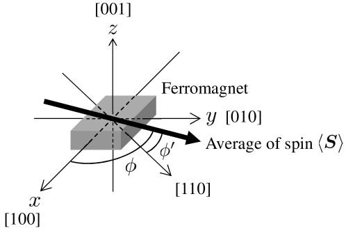
Figure 1: Sketch of the sample geometry. The tetragonal distortion is in the [001] direction. The current $I$ flows in the [100], [110], or [001] direction. The thermal average of the spin $\langle{\mbox{\boldmath$S$}}\rangle$ ($\propto$$-{\mbox{\boldmath$M$}}$) lies in the (001) plane. For $\phi_{i}$, we set $\phi_{[100]}=\phi_{[001]}=\phi$ and $\phi_{[110]}=\phi^{\prime}$. Here, $\phi$ is the relative angle between $\langle{\mbox{\boldmath$S$}}\rangle$ and the [100] direction, and $\phi^{\prime}$ is the relative angle between the $\langle{\mbox{\boldmath$S$}}\rangle$ direction and the [110] direction. The relation between $\phi$ and $\phi^{\prime}$ is given by Eq. (5). Furthermore, the $x$-, $y$-, and $z$-axes are specified to describe the Hamiltonian of Eq. (6).

2.2 Hamiltonian

Following our previous study[27, 28], we consider ${\cal H}$ as the Hamiltonian of the localized d states of a single atom in a ferromagnet with a spin–orbit interaction, an exchange field, and a crystal field of tetragonal symmetry. This crystal field represents the case that a distortion in the [001] direction is added to a crystal field of cubic symmetry. The reason for choosing this crystal field is that $C_{4}^{[100]}$ appears under the crystal field of tetragonal symmetry, whereas it takes a value of almost 0 under the crystal field of cubic symmetry, as reported in Refs. Kokado3 and others. The Hamiltonian ${\cal H}$ is expressed as

$${\cal H}={\cal H}_{0}+V,$$ (6)

$${\cal H}_{0}={\cal H}_{\rm cubic}-{\mbox{\boldmath$S$}}\cdot{\mbox{\boldmath$H$}},$$ (7)

$$V=V_{\rm so}+V_{\rm tetra},$$ (8)

where

$${\cal H}_{\rm cubic}=\sum_{\sigma=\pm}\Bigg{[}E_{\varepsilon}\Big{(}|xy,\chi_{\sigma}(\phi)\rangle\langle xy,\chi_{\sigma}(\phi)|+|yz,\chi_{\sigma}(\phi)\rangle\langle yz,\chi_{\sigma}(\phi)|+|xz,\chi_{\sigma}(\phi)\rangle\langle xz,\chi_{\sigma}(\phi)|\Big{)}$$

$$\hskip 42.67912pt+E_{\gamma}\Big{(}|x^{2}-y^{2},\chi_{\sigma}(\phi)\rangle\langle x^{2}-y^{2},\chi_{\sigma}(\phi)|+|3z^{2}-r^{2},\chi_{\sigma}(\phi)\rangle\langle 3z^{2}-r^{2},\chi_{\sigma}(\phi)|\Big{)}\Bigg{]},$$ (9)

$$V_{\rm so}=\lambda{\mbox{\boldmath$L$}}\cdot{\mbox{\boldmath$S$}},$$ (10)

$$V_{\rm tetra}=\sum_{\sigma=\pm}\Bigg{[}\delta_{\varepsilon}\Big{(}|xz,\chi_{\sigma}(\phi)\rangle\langle xz,\chi_{\sigma}(\phi)|+|yz,\chi_{\sigma}(\phi)\rangle\langle yz,\chi_{\sigma}(\phi)|\Big{)}$$

$$\hskip 42.67912pt+\delta_{\gamma}|3z^{2}-r^{2},\chi_{\sigma}(\phi)\rangle\langle 3z^{2}-r^{2},\chi_{\sigma}(\phi)|\Bigg{]},$$ (11)

and

$${\mbox{\boldmath$S$}}=(S_{x},S_{y},S_{z}),$$ (12)

$${\mbox{\boldmath$L$}}=(L_{x},L_{y},L_{z}),$$ (13)

$${\mbox{\boldmath$H$}}=H\left(\cos\phi,\sin\phi,0\right).$$ (14)

The above terms are explained as follows. The term ${\cal H}_{\rm cubic}$ represents the crystal field of cubic symmetry. The term $-{\mbox{\boldmath$S$}}\cdot{\mbox{\boldmath$H$}}$ is the Zeeman interaction between the spin angular momentum $S$ and the exchange field of the ferromagnet $H$, where ${\mbox{\boldmath$H$}}\propto-{\mbox{\boldmath$M$}}$, ${\mbox{\boldmath$H$}}\propto\langle{\mbox{\boldmath$S$}}\rangle$, and $H>0$. The term $V_{\rm so}$ is the spin–orbit interaction, where $\lambda$ is the spin–orbit coupling constant and $L$ is the orbital angular momentum. The spin quantum number $S$ and the azimuthal quantum number $L$ are chosen to be $S=1/2$ and $L=2$.[25] The term $V_{\rm tetra}$ is an additional term to reproduce the crystal field of tetragonal symmetry. The state $|m,\chi_{\sigma}(\phi)\rangle$ is expressed by $|m,\chi_{\sigma}(\phi)\rangle=|m\rangle|\chi_{\sigma}(\phi)\rangle$. The state $|m\rangle$ is the orbital state, defined by $|xy\rangle=xyf(r)$, $|yz\rangle=yzf(r)$, $|xz\rangle=xzf(r)$, $|x^{2}-y^{2}\rangle=(1/2)(x^{2}-y^{2})f(r)$, and $|3z^{3}-r^{2}\rangle=[1/(2\sqrt{3})](3z^{2}-r^{2})f(r)$, with $r=\sqrt{x^{2}+y^{2}+z^{2}}$ and $f(r)=\Gamma e^{-\zeta r}$, where $f(r)$ is the radial part of the 3d orbital, and $\Gamma$ and $\zeta$ are constants. The states $|xy\rangle$, $|yz\rangle$, and $|xz\rangle$ are called $d\varepsilon$ orbitals and $|x^{2}-y^{2}\rangle$ and $|3z^{2}-r^{2}\rangle$ are $d\gamma$ orbitals. The quantity $E_{\varepsilon}$ is the energy level of $|xy\rangle$, and $E_{\gamma}$ is that of $|x^{2}-y^{2}\rangle$. The quantity $\Delta$ is defined as $\Delta$=$E_{\gamma}-E_{\varepsilon}$, $\delta_{\varepsilon}$ is the energy difference between $|xz\rangle$ (or $|yz\rangle$) and $|xy\rangle$, and $\delta_{\gamma}$ is that between $|3z^{2}-r^{2}\rangle$ and $|x^{2}-y^{2}\rangle$ (see Fig. 2). The state $|\chi_{\sigma}(\phi)\rangle$ ($\sigma=+$ and $-$) is the spin state, i.e.,

$$|\chi_{+}(\phi)\rangle=\frac{1}{\sqrt{2}}\left(e^{-i\phi}|\uparrow\rangle+|\downarrow\rangle\right),$$ (15)

$$|\chi_{-}(\phi)\rangle=\frac{1}{\sqrt{2}}\left(-e^{-i\phi}|\uparrow\rangle+|\downarrow\rangle\right),$$ (16)

which are eigenstates of $-{\mbox{\boldmath$S$}}\cdot{\mbox{\boldmath$H$}}$. Here, $|\chi_{+}(\phi)\rangle$ ($|\chi_{-}(\phi)\rangle$) denotes the up spin state (down spin state) for the case in which the quantization axis is chosen along the $\langle{\mbox{\boldmath$S$}}\rangle$ direction. The state $|\uparrow\rangle$ ($|\downarrow\rangle$) represents the up spin state (down spin state) for the case in which the quantization axis is chosen along the $z$-axis. For ${\cal H}$ of Eq. (6), we also assume the relation of parameters for typical ferromagnets, i.e., $\Delta/H\ll 1$[27], $|\lambda|/\Delta\ll 1$, $\delta_{\varepsilon}/\Delta\ll 1$, and $\delta_{\gamma}/\Delta\ll 1$.

On the basis of the relation of the parameters, we consider ${\cal H}_{0}$ of Eq. (7) and $V$ of Eq. (8) as the unperturbed term and the perturbed term, respectively. When the matrix of ${\cal H}$ of Eq. (6) is represented in the basis set $|xy,\chi_{\pm}(\phi)\rangle$, $|yz,\chi_{\pm}(\phi)\rangle$, $|xz,\chi_{\pm}(\phi)\rangle$, $|x^{2}-y^{2},\chi_{\pm}(\phi)\rangle$, and $|3z^{2}-r^{2},\chi_{\pm}(\phi)\rangle$, the unperturbed system is degenerate (see Table A$\cdot$I in Ref. Kokado3). We therefore use the perturbation theory for the case in which the unperturbed system is degenerate.[36, 37] As a result, we choose the following basis set for the subspace with $|xy,\chi_{\pm}(\phi)\rangle$, $|yz,\chi_{\pm}(\phi)\rangle$, and $|xz,\chi_{\pm}(\phi)\rangle$:[27]

$$|\xi_{+},\chi_{+}(\phi)\rangle=A\Big{[}(\delta_{\varepsilon}-\sqrt{\delta_{\varepsilon}^{2}+\lambda^{2}})|xy,\chi_{+}(\phi)\rangle+i\lambda\sin\phi|yz,\chi_{+}(\phi)\rangle-i\lambda\cos\phi|xz,\chi_{+}(\phi)\rangle\Big{]},$$

(17)

$$|\delta_{\varepsilon},\chi_{+}(\phi)\rangle=\cos\phi|yz,\chi_{+}(\phi)\rangle+\sin\phi|xz,\chi_{+}(\phi)\rangle,$$ (18)

$$|\xi_{-},\chi_{+}(\phi)\rangle=B\Big{[}(\delta_{\varepsilon}+\sqrt{\delta_{\varepsilon}^{2}+\lambda^{2}})|xy,\chi_{+}(\phi)\rangle+i\lambda\sin\phi|yz,\chi_{+}(\phi)\rangle-i\lambda\cos\phi|xz,\chi_{+}(\phi)\rangle\Big{]},$$

(19)

$$|\xi_{+},\chi_{-}(\phi)\rangle=A\Big{[}(\delta_{\varepsilon}-\sqrt{\delta_{\varepsilon}^{2}+\lambda^{2}})|xy,\chi_{-}(\phi)\rangle-i\lambda\sin\phi|yz,\chi_{-}(\phi)\rangle+i\lambda\cos\phi|xz,\chi_{-}(\phi)\rangle\Big{]},$$

(20)

$$|\delta_{\varepsilon},\chi_{-}(\phi)\rangle=\cos\phi|yz,\chi_{-}(\phi)\rangle+\sin\phi|xz,\chi_{-}(\phi)\rangle,$$ (21)

$$|\xi_{-},\chi_{-}(\phi)\rangle=B\Big{[}(\delta_{\varepsilon}+\sqrt{\delta_{\varepsilon}^{2}+\lambda^{2}})|xy,\chi_{-}(\phi)\rangle-i\lambda\sin\phi|yz,\chi_{-}(\phi)\rangle+i\lambda\cos\phi|xz,\chi_{-}(\phi)\rangle\Big{]},$$

with

$$\xi_{\pm}=\frac{1}{2}\left(\delta_{\varepsilon}\pm\sqrt{\delta_{\varepsilon}^{2}+\lambda^{2}}\right),$$ (23)

$$A=\left(2\delta_{\varepsilon}^{2}+2\lambda^{2}-2\delta_{\varepsilon}\sqrt{\delta_{\varepsilon}^{2}+\lambda^{2}}\right)^{-1/2},$$ (24)

$$B=\left(2\delta_{\varepsilon}^{2}+2\lambda^{2}+2\delta_{\varepsilon}\sqrt{\delta_{\varepsilon}^{2}+\lambda^{2}}\right)^{-1/2}.$$ (25)

Using $|\xi_{+},\chi_{\pm}(\phi)\rangle$, $|\delta_{\varepsilon},\chi_{\pm}(\phi)\rangle$, $|\xi_{-},\chi_{\pm}(\phi)\rangle$, $|x^{2}-y^{2},\chi_{\pm}(\phi)\rangle$, and $|3z^{2}-r^{2},\chi_{\pm}(\phi)\rangle$, we construct the matrix of ${\cal H}$ of Eq. (6) as shown in Table I in Ref. Kokado3.

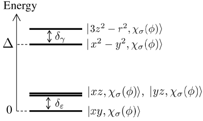
Figure 2: Energy levels of the 3d states in the crystal field of tetragonal symmetry.[35] The second excited states are doubly degenerate. The energy levels are measured from the energy level of $|xy\rangle$, $E_{\varepsilon}$.

2.3 Localized d states

Applying the first- and second-order perturbation theory to ${\cal H}$ in Table I in Ref. Kokado3, we obtain the localized d state $|m,\chi_{\varsigma}(\phi))$, with $m=\xi_{+}$, $\delta_{\varepsilon}$, $\xi_{-}$, $x^{2}-y^{2}$, and $3z^{2}-r^{2}$ and $\varsigma=+$ and $-$, where $m$ ($\varsigma$) denotes the orbital index (spin index) of the dominant state in $|m,\chi_{\varsigma}(\phi))$ [see Eq. (B)]. In general, $|m,\chi_{\varsigma}(\phi))$ is written as

$$|m,\chi_{\varsigma}(\phi))=\left[1-c_{m,\varsigma}(\phi)\right]|m,\chi_{\varsigma}(\phi)\rangle+\sum_{n~{}(\neq m)}\sum_{\sigma=+,-}c_{n,\sigma}^{m,\varsigma}(\phi)|n,\chi_{\sigma}(\phi)\rangle,$$ (26)

with $c_{m,\varsigma}(\phi)>0$. Here, $|m,\chi_{\varsigma}(\phi)\rangle$ is the dominant state and $|n,\chi_{\sigma}(\phi)\rangle$ is the slightly hybridized state due to $V_{\rm so}$. The coefficient $1-c_{m,\varsigma}(\phi)$ [$c_{n,\sigma}^{m,\varsigma}(\phi)$] represents the probability amplitude of $|m,\chi_{\varsigma}(\phi)\rangle$ [$|n,\chi_{\sigma}(\phi)\rangle$], where $-c_{m,\varsigma}(\phi)$ means the reduction of the probability amplitude of $|m,\chi_{\varsigma}(\phi)\rangle$. In simple terms, $c_{m,\varsigma}(\phi)$ and $c_{n,\sigma}^{m,\varsigma}(\phi)$ represent the change in the d state due to $V_{\rm so}$, where $c_{m,\varsigma}(\phi)$ and $c_{n,\sigma}^{m,\varsigma}(\phi)$ are 0 at $\lambda=0$. Note that $|m,\chi_{\varsigma}(\phi))$ is expressed up to the second order of $\lambda/H$, $\lambda/\Delta$, $\lambda/(H\pm\Delta)$, $\delta_{t}/H$, $\delta_{t}/\Delta$, and $\delta_{t}/(H\pm\Delta)$, with $t=\varepsilon$ or $\gamma$.

2.4 Resistivity

Using Eq. (26), we can obtain an expression for $\rho^{i}(\phi)$. The resistivity $\rho^{i}(\phi)$ is described by the two-current model,[3] i.e.,

$$\rho^{i}(\phi)=\frac{\rho_{+}^{i}(\phi)\rho_{-}^{i}(\phi)}{\rho_{+}^{i}(\phi)+\rho_{-}^{i}(\phi)}.$$ (27)

The quantity $\rho_{\sigma}^{i}(\phi)$ is the resistivity of the $\sigma$ spin at $\phi$ in the case of $i$, where $\sigma=+$ ($-$) denotes the up spin (down spin) for the case in which the quantization axis is chosen along the direction of $\langle{\mbox{\boldmath$S$}}\rangle$ [see Eqs. (15) and (16)]. The resistivity $\rho_{\sigma}^{i}(\phi)$ is written as

$$\rho_{\sigma}^{i}(\phi)=\frac{m_{\sigma}^{*}}{n_{\sigma}e^{2}\tau_{\sigma}^{i}(\phi)},$$ (28)

where $e$ is the electric charge and $n_{\sigma}$ ($m^{*}_{\sigma}$) is the number density (effective mass) of the electrons in the conduction band of the $\sigma$ spin.[38, 39] The conduction band consists of the s, p, and conductive d states.[25] In addition, $1/\tau_{\sigma}^{i}(\phi)$ is the scattering rate of the conduction electron of the $\sigma$ spin in the case of $i$, expressed as

$$\frac{1}{\tau_{\sigma}^{i}(\phi)}=\frac{1}{\tau_{s,\sigma}}+\sum_{m}\sum_{\varsigma=+,-}\frac{1}{\tau_{s,\sigma\to m,\varsigma}^{i}(\phi)},$$ (29)

with

$$\frac{1}{\tau_{s,\sigma\to m,\varsigma}^{i}(\phi)}=\frac{2\pi}{\hbar}n_{\rm imp}N_{\rm n}{V_{\rm imp}(R_{\rm n})}^{2}\left|(m,\chi_{\varsigma}(\phi)|e^{i{\mbox{\boldmath$k$}}_{\sigma}^{i}\cdot{\mbox{\boldmath$r$}}},\chi_{\sigma}(\phi)\rangle\right|^{2}D_{m,\varsigma}^{(d)}.$$ (30)

Here, $1/\tau_{s,\sigma}$ is the $s$–$s$ scattering rate, which is considered to be independent of $i$. The $s$–$s$ scattering means that the conduction electron of the $\sigma$ spin is scattered into the conduction state of the $\sigma$ spin by nonmagnetic impurities and phonons. The quantity $1/\tau_{s,\sigma\to m,\varsigma}^{i}(\phi)$ is the $s$–$d$ scattering rate in the case of $i$.[25, 26] The $s$–$d$ scattering means that the conduction electron of the $\sigma$ spin is scattered into the $\sigma$ spin state in $|m,\chi_{\varsigma}(\phi))$ of Eq. (26) by nonmagnetic impurities. The quantity $D_{m,\varsigma}^{(d)}$ represents the partial density of states (PDOS) of the wave function of the tight-binding model for the d state of the $m$ orbital and $\varsigma$ spin at the Fermi energy $E_{\mbox{\tiny F}}$, as described in Appendix B in Ref. Kokado1. The conduction state of the $\sigma$ spin $|e^{i{\mbox{\boldmath$k$}}_{\sigma}^{i}\cdot{\mbox{\boldmath$r$}}},\chi_{\sigma}(\phi)\rangle$ is represented by the plane wave, i.e.,

$$|e^{i{\mbox{\boldmath$k$}}_{\sigma}^{i}\cdot{\mbox{\boldmath$r$}}},\chi_{\sigma}(\phi)\rangle=\frac{1}{\sqrt{\Omega}}e^{i{\mbox{\boldmath$k$}}_{\sigma}^{i}\cdot{\mbox{\boldmath$r$}}}\chi_{\sigma}(\phi),$$ (31)

where ${\mbox{\boldmath$k$}}_{\sigma}^{i}$ [=$(k_{x,\sigma}^{i},k_{y,\sigma}^{i},k_{z,\sigma}^{i})$] is the Fermi wave vector of the $\sigma$ spin in the $i$ direction, $r$ is the position of the conduction electron, and $\Omega$ is the volume of the system. The quantity $V_{\rm imp}(R_{\rm n})$ is the scattering potential at $R_{\rm n}$ due to a single impurity, where $R_{\rm n}$ is the distance between the impurity and the nearest-neighbor host atom.[25] The quantity $N_{\rm n}$ is the number of nearest-neighbor host atoms around a single impurity,[25] $n_{\rm imp}$ is the number density of impurities, and $\hbar$ is the Planck constant $h$ divided by 2$\pi$.

We calculate the overlap integral $\langle m,\chi_{\sigma}(\phi)|e^{i{\mbox{\boldmath$k$}}_{\sigma}^{i}\cdot{\mbox{\boldmath$r$}}},\chi_{\sigma}(\phi)\rangle$ in Eq. (30) using Eq. (C$\cdot$1) in Ref. Kokado3. The overlap integrals of ${\mbox{\boldmath$I$}}//[100]$, ${\mbox{\boldmath$I$}}//[110]$, and ${\mbox{\boldmath$I$}}//[001]$ are as follows:

1. ${\mbox{\boldmath$I$}}//[100]$
   In the case of ${\mbox{\boldmath$I$}}//[100]$ corresponding to ${\mbox{\boldmath$k$}}_{\sigma}^{[100]}=(k_{\sigma},0,0)$, the overlap integral becomes

   $$\langle xy,\chi_{\sigma^{\prime}}(\phi)|e^{ik_{\sigma}x},\chi_{\sigma}(\phi)\rangle=\langle yz,\chi_{\sigma^{\prime}}(\phi)|e^{ik_{\sigma}x},\chi_{\sigma}(\phi)\rangle=\langle xz,\chi_{\sigma^{\prime}}(\phi)|e^{ik_{\sigma}x},\chi_{\sigma}(\phi)\rangle=0,$$

   (32)

   $$\langle x^{2}-y^{2},\chi_{\sigma^{\prime}}(\phi)|e^{ik_{\sigma}x},\chi_{\sigma}(\phi)\rangle=\frac{1}{2}g_{\sigma}\delta_{\sigma,\sigma^{\prime}},$$ (33)

   $$\langle 3z^{2}-r^{2},\chi_{\sigma^{\prime}}(\phi)|e^{ik_{\sigma}x},\chi_{\sigma}(\phi)\rangle=-\frac{1}{2\sqrt{3}}g_{\sigma}\delta_{\sigma,\sigma^{\prime}},$$ (34)

   with

   $$g_{\sigma}=-\frac{192\pi\Gamma\zeta k_{\sigma}^{2}}{\sqrt{\Omega}(k_{\sigma}^{2}+\zeta^{2})^{4}}.$$ (35)

   The scatterings from the plane wave to $|3z^{2}-r^{2},\chi_{\sigma}(\phi)\rangle$ and $|x^{2}-y^{2},\chi_{\sigma}(\phi)\rangle$ are thus allowed. Using Eqs. ((i)) and (2.2)$-$(2.2), we also have

   $$\langle\xi_{+},\chi_{\sigma^{\prime}}(\phi)|e^{ik_{\sigma}x},\chi_{\sigma}(\phi)\rangle=\langle\delta_{\varepsilon},\chi_{\sigma^{\prime}}(\phi)|e^{ik_{\sigma}x},\chi_{\sigma}(\phi)\rangle=\langle\xi_{-},\chi_{\sigma^{\prime}}(\phi)|e^{ik_{\sigma}x},\chi_{\sigma}(\phi)\rangle=0.$$ (36)

2. ${\mbox{\boldmath$I$}}//[110]$
   In the case of ${\mbox{\boldmath$I$}}//[110]$ corresponding to ${\mbox{\boldmath$k$}}_{\sigma}^{[110]}=(k_{\sigma},k_{\sigma},0)/\sqrt{2}$, the overlap integral is

   $$\langle xy,\chi_{\sigma^{\prime}}(\phi)|e^{i(k_{\sigma}x+k_{\sigma}y)/\sqrt{2}},\chi_{\sigma}(\phi)\rangle=\frac{1}{2}g_{\sigma}\delta_{\sigma,\sigma^{\prime}},$$ (37)

   $$\langle yz,\chi_{\sigma^{\prime}}(\phi)|e^{i(k_{\sigma}x+k_{\sigma}y)/\sqrt{2}},\chi_{\sigma}(\phi)\rangle=\langle xz,\chi_{\sigma^{\prime}}(\phi)|e^{i(k_{\sigma}x+k_{\sigma}y)/\sqrt{2}},\chi_{\sigma}(\phi)\rangle=0,$$

   (38)

   $$\langle x^{2}-y^{2},\chi_{\sigma^{\prime}}(\phi)|e^{i(k_{\sigma}x+k_{\sigma}y)/\sqrt{2}},\chi_{\sigma}(\phi)\rangle=0,$$ (39)

   $$\langle 3z^{2}-r^{2},\chi_{\sigma^{\prime}}(\phi)|e^{i(k_{\sigma}x+k_{\sigma}y)/\sqrt{2}},\chi_{\sigma}(\phi)\rangle=-\frac{1}{2\sqrt{3}}g_{\sigma}\delta_{\sigma,\sigma^{\prime}}.$$ (40)

   The scatterings from the plane wave to $|xy,\chi_{\sigma}(\phi)\rangle$ and $|3z^{2}-r^{2},\chi_{\sigma}(\phi)\rangle$ are thus allowed. Using Eqs. (37), ((ii)), and (2.2)$-$(2.2), we also have

   $$\langle\xi_{+},\chi_{\sigma^{\prime}}(\phi)|e^{i(k_{\sigma}x+k_{\sigma}y)/\sqrt{2}},\chi_{\sigma}(\phi)\rangle=\frac{1}{2}A\left(\delta_{e}-\sqrt{\delta_{e}^{2}+\lambda^{2}}\right)g_{\sigma}\delta_{\sigma,\sigma^{\prime}},$$ (41)

   $$\langle\delta_{\varepsilon},\chi_{\sigma^{\prime}}(\phi)|e^{i(k_{\sigma}x+k_{\sigma}y)/\sqrt{2}},\chi_{\sigma}(\phi)\rangle=0,$$ (42)

   $$\langle\xi_{-},\chi_{\sigma^{\prime}}(\phi)|e^{i(k_{\sigma}x+k_{\sigma}y)/\sqrt{2}},\chi_{\sigma}(\phi)\rangle=\frac{1}{2}B\left(\delta_{e}+\sqrt{\delta_{e}^{2}+\lambda^{2}}\right)g_{\sigma}\delta_{\sigma,\sigma^{\prime}},$$ (43)

   where $A$ and $B$ have been given by Eqs. (24) and (25), respectively.

3. ${\mbox{\boldmath$I$}}//[001]$
   In the case of ${\mbox{\boldmath$I$}}//[001]$ corresponding to ${\mbox{\boldmath$k$}}_{\sigma}^{[001]}=(0,0,k_{\sigma})$, the overlap integral is

   $$\langle xy,\chi_{\sigma^{\prime}}(\phi)|e^{ik_{\sigma}z},\chi_{\sigma}(\phi)\rangle=\langle yz,\chi_{\sigma^{\prime}}(\phi)|e^{ik_{\sigma}z},\chi_{\sigma}(\phi)\rangle=\langle xz,\chi_{\sigma^{\prime}}(\phi)|e^{ik_{\sigma}z},\chi_{\sigma}(\phi)\rangle=0,$$

   (44)

   $$\langle x^{2}-y^{2},\chi_{\sigma^{\prime}}(\phi)|e^{ik_{\sigma}z},\chi_{\sigma}(\phi)\rangle=0,$$ (45)

   $$\langle 3z^{2}-r^{2},\chi_{\sigma^{\prime}}(\phi)|e^{ik_{\sigma}z},\chi_{\sigma}(\phi)\rangle=\frac{1}{\sqrt{3}}g_{\sigma}\delta_{\sigma,\sigma^{\prime}}.$$ (46)

   Only the scattering from the plane wave to $|3z^{2}-r^{2},\chi_{\sigma}(\phi)\rangle$ is thus allowed. Using Eqs. ((iii)) and (2.2)$-$(2.2), we also have

   $$\langle\xi_{+},\chi_{\sigma^{\prime}}(\phi)|e^{ik_{\sigma}z},\chi_{\sigma}(\phi)\rangle=\langle\delta_{\varepsilon},\chi_{\sigma^{\prime}}(\phi)|e^{ik_{\sigma}z},\chi_{\sigma}(\phi)\rangle=\langle\xi_{-},\chi_{\sigma^{\prime}}(\phi)|e^{ik_{\sigma}z},\chi_{\sigma}(\phi)\rangle=0.$$ (47)

Substituting the above results into Eq. (30), we obtain the expression for $\rho_{\sigma}^{i}(\phi)$ of Eq. (28) as shown in Appendix C. Here, $\rho_{\sigma}^{i}(\phi)$ is expressed by using the following quantities[26]:

$$\rho_{s,\sigma}=\frac{m_{\sigma}^{*}}{n_{\sigma}e^{2}\tau_{s,\sigma}},$$ (48)

$$\rho_{s,\sigma\to m,\varsigma}=\frac{m_{\sigma}^{*}}{n_{\sigma}e^{2}\tau_{s,\sigma\to m,\varsigma}},$$ (49)

where $\rho_{s,\sigma}$ is the $s$–$s$ resistivity and $\rho_{s,\sigma\to m,\varsigma}$ is the $s$–$d$ resistivity. The $s$–$d$ scattering rate $1/\tau_{s,\sigma\to m,\varsigma}$ is defined by

$$\frac{1}{\tau_{s,\sigma\to m,\varsigma}}=\frac{2\pi}{\hbar}n_{\rm imp}N_{\rm n}{V_{\rm imp}(R_{\rm n})}^{2}\left|\langle 3z^{2}-r^{2},\chi_{\sigma}(\phi)|e^{ik_{\sigma}z},\chi_{\sigma}(\phi)\rangle\right|^{2}D_{m,\varsigma}^{(d)}$$

$$\hskip 42.67912pt=\frac{2\pi}{\hbar}n_{\rm imp}N_{\rm n}\frac{1}{3}v_{\sigma}^{2}D_{m,\varsigma}^{(d)},$$ (50)

with

$$v_{\sigma}=V_{\rm imp}(R_{\rm n})g_{\sigma},$$ (51)

where $g_{\sigma}$ is given by Eq. (35). The overlap integral $\langle 3z^{2}-r^{2},\chi_{\sigma}(\phi)|e^{ik_{\sigma}z},\chi_{\sigma}(\phi)\rangle$ in Eq. (2.4) can be calculated by using Eq. (C$\cdot$1) in Ref. Kokado3. Here, Eq. (2.4) has been introduced to investigate the relation between the present result and the previous ones[3, 25, 26] (also see Appendix G).

We also note that, as found from Eq. (2.4), $\rho_{s,\sigma\to m,\varsigma}$ of Eq .(49) satisfies

$$\rho_{s,\sigma\to m,\varsigma}\propto D_{m,\varsigma}^{(d)}.$$ (52)

This relation is useful to give a physical explanation for $C_{j}^{i}$.

3 Application

We apply the theory of Sect. 2 to ferromagnets with $D_{m,+}^{(d)}=0$ and $D_{m,-}^{(d)}\neq 0$. Using $\rho_{\sigma}^{i}(\phi_{i})$ in Appendix C, we obtain AMR${}^{i}(\phi_{i})$ of Eq. (1) for the ferromagnets. The AMR ratio AMR${}^{i}(\phi_{i})$ is expressed up to the second order of $\lambda/H$, $\lambda/\Delta$, $\lambda/(H\pm\Delta)$, $\delta_{t}/H$, $\delta_{t}/\Delta$, and $\delta_{t}/(H\pm\Delta)$, with $t=\varepsilon$ or $\gamma$. Here, we introduce

$$r=\frac{\rho_{s,-}}{\rho_{s,+}},$$ (53)

$$r_{s,\sigma\to m,-}=\frac{\rho_{s,\sigma\to m,-}}{\rho_{s,+}},$$ (54)

in accordance with our previous study[26]. In addition, we set

$$r_{s,\sigma\to\delta_{\varepsilon},-}\equiv r_{s,\sigma\to\varepsilon 1,-},$$ (55)

$$r_{s,\sigma\to\xi_{+},-}=r_{s,\sigma\to\xi_{-},-}\equiv r_{s,\sigma\to\varepsilon 2,-},$$ (56)

for simplicity.

3.1 ${\mbox{\boldmath$I$}}//[100]$

Using Eqs. (1), (27), and (86), we obtain ${\rm AMR}^{[100]}(\phi)$:

$${\rm AMR}^{[100]}(\phi)=C_{0}^{[100]}+C_{2}^{[100]}\cos 2\phi+C_{4}^{[100]}\cos 4\phi.$$ (57)

Here, $C_{0}^{[100]}$ is determined so as to satisfy ${\rm AMR}^{[100]}(\pi/2)=0$. In addition, $C_{2}^{[100]}$ and $C_{4}^{[100]}$ are expressed as Eqs. (D.1) and (D.1), respectively. Using Eqs. (D.1) and (D.1), Eq. (43) in Ref. Kokado3, Eq. (45) in Ref. Kokado3, Eq. (46) in Ref. Kokado3, Eq. (2) in Ref. Kokado3_1, and Eq. (3) in Ref. Kokado3_1, we derive expressions for $C_{2}^{[100]}$ and $C_{4}^{[100]}$, where $\rho_{s,\sigma\to m,+}=0$ due to $D_{m,+}^{(d)}=0$ is taken into account. The respective expressions are given in Sect. E.1.

3.2 ${\mbox{\boldmath$I$}}//[110]$

Using Eqs. (1), (27), and (92), we obtain ${\rm AMR}^{[110]}(\phi^{\prime})$:

$${\rm AMR}^{[110]}(\phi^{\prime})=C_{0}^{[110]}+C_{2}^{[110]}\cos 2\phi^{\prime}+C_{4}^{[110]}\cos 4\phi^{\prime}+C_{6}^{[110]}\cos 6\phi^{\prime}+C_{8}^{[110]}\cos 8\phi^{\prime}.$$ (58)

Here, $C_{0}^{[110]}$ is determined so as to satisfy ${\rm AMR}^{[110]}(\pi/2)=0$. In addition, $C_{2}^{[110]}$, $C_{4}^{[110]}$, $C_{6}^{[110]}$, and $C_{8}^{[110]}$ are expressed as Eqs. (124), (124), (126), and (126), respectively. Using Eqs. (124)$-$(126), (100), (101), and (104)$-$(109), we derive expressions for $C_{2}^{[110]}$, $C_{4}^{[110]}$, $C_{6}^{[110]}$, and $C_{8}^{[110]}$. The respective expressions are given in Sect. E.2.

3.3 ${\mbox{\boldmath$I$}}//[001]$

Using Eqs. (1), (27), and (110), we obtain ${\rm AMR}^{[001]}(\phi)$:

$${\rm AMR}^{[001]}(\phi)=C_{0}^{[001]}+C_{4}^{[001]}\cos 4\phi.$$ (59)

Here, $C_{0}^{[001]}$ is determined so as to satisfy ${\rm AMR}^{[001]}(\pi/2)=0$. In addition, $C_{4}^{[001]}$ is expressed as Eq. (127). Using Eqs. (127), (113), (114), (117), and (C.3), we derive an expression for $C_{4}^{[001]}$. The respective expressions are given in Sect. E.3. Note that the feature that the $\phi$-dependent term is only the $\cos 4\phi$ term is also found in the expression by D$\ddot{\rm o}$ring,[32] i.e., Eq. (73).

3.4 Simplified system

On the basis of the above-mentioned $C_{j}^{i}$, we obtain a simple expression for $C_{j}^{i}$ for the simplified system. In this system, we assume

$$r_{s,-\to x^{2}-y^{2},-}=r_{s,-\to 3z^{2}-r^{2},-}\equiv r_{s,-\to\gamma,-},$$ (60)

which corresponds to $\rho_{s,-\to x^{2}-y^{2},-}=\rho_{s,-\to 3z^{2}-r^{2},-}$, i.e., $D_{x^{2}-y^{2},-}^{(d)}=D_{3z^{2}-r^{2},-}^{(d)}$ [see Eqs. (54) and (52)]. This assumption may be valid for the system of $D_{x^{2}-y^{2},-}^{(d)}\sim D_{3z^{2}-r^{2},-}^{(d)}$ and/or $|\lambda|/\delta_{\gamma}\ll 1$. The reason is that the terms with $r_{s,-\to 3z^{2}-r^{2},-}-r_{s,-\to x^{2}-y^{2},-}$ in $C_{j}^{i}$ have $\left(\frac{\lambda}{\delta_{\gamma}}\right)\left(r_{s,-\to 3z^{2}-r^{2},-}-r_{s,-\to x^{2}-y^{2},-}\right)$, $\left(\frac{\lambda}{\delta_{\gamma}}\right)^{2}\left(r_{s,-\to 3z^{2}-r^{2},-}-r_{s,-\to x^{2}-y^{2},-}\right)$, and $\left(\frac{\lambda}{\delta_{\gamma}}\right)^{2}\left(r_{s,-\to 3z^{2}-r^{2},-}-r_{s,-\to x^{2}-y^{2},-}\right)^{2}$. We also use $(\frac{\lambda}{H\pm\Delta})^{2}\approx\left(\frac{\lambda}{H}\right)^{2}$, $\frac{\lambda^{2}}{\Delta(H\pm\Delta)}\approx\frac{\lambda^{2}}{H\Delta}\mp\left(\frac{\lambda}{H}\right)^{2}$, and $\frac{\lambda^{2}}{H(H\pm\Delta)}\approx\left(\frac{\lambda}{H}\right)^{2}$ due to $\Delta/H\ll 1$.

For this system, we consider three types:

1. type A: generalized strong ferromagnet with the $s$–$d$ scattering “$s,+\to d,-$ and $s,-\to d,-$”,

2. type B: half-metallic ferromagnet with the dominant $s$–$d$ scattering “$s,-\to d,-$”, and

3. type C: specified strong ferromagnet with the dominant $s$–$d$ scattering “$s,+\to d,-$”.

In Tables 1, 2, and 3, we show $C_{j}^{i}$ for types A, B, and C, respectively. The coefficient $C_{j}^{i}$ for type A is derived by imposing Eq. (60) on Eqs. (128)$-$(E.1), (132)$-$(135), (136), and (E.3). The coefficient $C_{j}^{i}$ for type B is obtained by imposing $r\ll 1$, $r_{s,\sigma\to\varepsilon 1,-}\ll 1$, $r_{s,\sigma\to\varepsilon 2,-}\ll 1$, and $r_{s,\sigma\to\gamma,-}\ll 1$ on $C_{j}^{i}$ for type A in Table 1. The coefficient $C_{j}^{i}$ for type C is obtained by imposing $r\gg r_{s,\sigma\to\varepsilon 1,-}$, $r\gg r_{s,\sigma\to\varepsilon 2,-}$, $r\gg r_{s,\sigma\to\gamma,-}$, and $r\gg 1$ on $C_{j}^{i}$ for type A in Table 1, where $r$ is set to be large enough for the term including $r$ in the numerator to become dominant in each $C_{j}^{i}$ in spite of $\Delta/H\ll 1$. Note here that $C_{6}^{[110]}$ and $C_{8}^{[110]}$ are regarded as 0, because $C_{6}^{[110]}$ and $C_{8}^{[110]}$ in Table 1 include $r$ only in the respective denominators and then they become smaller than the other $C_{j}^{i}$.

We also mention that $C_{2}^{[100]}$ and $C_{4}^{[100]}$ for type A in Table 1 are, respectively, the coefficients in our previous study, i.e., Eqs. (61) and (62) in Ref. Kokado3, where $(\frac{\lambda}{H\pm\Delta})^{2}\approx(\frac{\lambda}{H})^{2}$ is used in this study. In addition, AMR${}^{[100]}(0)$ of Eq. (57) with $C_{2}^{[100]}$ in Table 1 and AMR${}^{[110]}(0)$ of Eq. (58) with $C_{2}^{[110]}$ and $C_{6}^{[110]}$ in Table 1 correspond to the CFJ model[3] under the condition of the CFJ model (see Appendix G).[40]

Table 1: The coefficient $C_{j}^{i}$ for type A, i.e., the generalized strong ferromagnet with the $s$–$d$ scattering “$s,+\to d,-$ and $s,-\to d,-$”. Type A has $D_{m,+}^{(d)}=0$, $D_{m,-}^{(d)}\neq 0$, $r_{s,\sigma\to\delta_{\varepsilon},-}\equiv r_{s,\sigma\to\varepsilon 1,-}$, $r_{s,\sigma\to\xi_{+},-}=r_{s,\sigma\to\xi_{-},-}\equiv r_{s,\sigma\to\varepsilon 2,-}$, $r_{s,\sigma\to 3z^{2}-r^{2},-}=r_{s,\sigma\to x^{2}-y^{2},-}\equiv r_{s,\sigma\to\gamma,-}$, and $\Delta/H\ll 1$. This $C_{j}^{i}$ is obtained by imposing $r_{s,\sigma\to 3z^{2}-r^{2},-}=r_{s,\sigma\to x^{2}-y^{2},-}\equiv r_{s,\sigma\to\gamma,-}$ and $\Delta/H\ll 1$ on Eqs. (128)$-$(E.3).

Coefficient
${\mbox{\boldmath$I$}}//[100]$
$C_{0}^{[100]}=C_{2}^{[100]}-C_{4}^{[100]}$
$C_{2}^{[100]}=\frac{3}{8}\frac{1}{1+r+r_{s,-\to\gamma,-}}\Bigg{[}\left(\frac{\lambda}{\Delta}\right)^{2}\frac{r_{s,-\to\gamma,-}-r_{s,-\to\varepsilon 1,-}}{r+r_{s,-\to\gamma,-}}-\left(\frac{\lambda}{H}\right)^{2}\frac{r_{s,-\to\gamma,-}}{r+r_{s,-\to\gamma,-}}+\left(\frac{\lambda}{H}\right)^{2}r_{s,+\to\varepsilon 2,-}(r+r_{s,-\to\gamma,-})\Bigg{]}$
$C_{4}^{[100]}=\frac{3}{32}\frac{1}{1+r+r_{s,-\to\gamma,-}}\Bigg{[}\left(\frac{\lambda}{\Delta}\right)^{2}\frac{r_{s,-\to\varepsilon 1,-}-r_{s,-\to\varepsilon 2,-}}{r+r_{s,-\to\gamma,-}}+\left(\frac{\lambda}{H}\right)^{2}(r_{s,+\to\varepsilon 2,-}-r_{s,+\to\varepsilon 1,-})(r+r_{s,-\to\gamma,-})\Bigg{]}$
${\mbox{\boldmath$I$}}//[110]$
$C_{0}^{[110]}=C_{2}^{[110]}-C_{4}^{[110]}+C_{6}^{[110]}-C_{8}^{[110]}$
$C_{2}^{[110]}=\frac{3}{8}\frac{1}{1+r+\frac{3}{4}r_{s,-\to\varepsilon 2,-}+\frac{1}{4}r_{s,-\to\gamma,-}}\Bigg{[}\left(\frac{\lambda}{\Delta}\right)^{2}\frac{\frac{3}{4}r_{s,-\to\varepsilon 1,-}+\frac{1}{4}r_{s,-\to\varepsilon 2,-}-r_{s,-\to\gamma,-}}{r+\frac{3}{4}r_{s,-\to\varepsilon 2,-}+\frac{1}{4}r_{s,-\to\gamma,-}}$
$+\frac{\lambda^{2}}{H\Delta}\frac{\frac{3}{4}r_{s,-\to\varepsilon 1,-}-\frac{7}{4}r_{s,-\to\varepsilon 2,-}+r_{s,-\to\gamma,-}}{r+\frac{3}{4}r_{s,-\to\varepsilon 2,-}+\frac{1}{4}r_{s,-\to\gamma,-}}+\frac{3}{4}\left(\frac{\lambda}{H}\right)^{2}\frac{r_{s,-\to\varepsilon 1,-}-r_{s,-\to\varepsilon 2,-}}{r+\frac{3}{4}r_{s,-\to\varepsilon 2,-}+\frac{1}{4}r_{s,-\to\gamma,-}}$
$-\left(\frac{\lambda}{H}\right)^{2}\frac{r_{s,-\to\gamma,-}}{r+\frac{3}{4}r_{s,-\to\varepsilon 2,-}+\frac{1}{4}r_{s,-\to\gamma,-}}+\left(\frac{\lambda}{H}\right)^{2}r_{s,+\to\varepsilon 1,-}\left(r+\frac{3}{4}r_{s,-\to\varepsilon 2,-}+\frac{1}{4}r_{s,-\to\gamma,-}\right)\Bigg{]}$
$C_{4}^{[110]}=\frac{3}{32}\frac{1}{1+r+\frac{3}{4}r_{s,-\to\varepsilon 2,-}+\frac{1}{4}r_{s,-\to\gamma,-}}\Bigg{[}\left(\frac{\lambda}{\Delta}\right)^{2}\frac{r_{s,-\to\varepsilon 2,-}-r_{s,-\to\varepsilon 1,-}}{r+\frac{3}{4}r_{s,-\to\varepsilon 2,-}+\frac{1}{4}r_{s,-\to\gamma,-}}$
$+\left(\frac{\lambda}{H}\right)^{2}(r_{s,+\to\varepsilon 1,-}-r_{s,+\to\varepsilon 2,-})\left(r+\frac{3}{4}r_{s,-\to\varepsilon 2,-}+\frac{1}{4}r_{s,-\to\gamma,-}\right)\Bigg{]}$
$C_{6}^{[110]}=\frac{9}{32}\left[\left(\frac{\lambda}{\Delta}\right)^{2}+\frac{\lambda^{2}}{H\Delta}+\left(\frac{\lambda}{H}\right)^{2}\right]\frac{r_{s,-\to\varepsilon 2,-}-r_{s,-\to\varepsilon 1,-}}{\left(r+\frac{3}{4}r_{s,-\to\varepsilon 2,-}+\frac{1}{4}r_{s,-\to\gamma,-}\right)\left(1+r+\frac{3}{4}r_{s,-\to\varepsilon 2,-}+\frac{1}{4}r_{s,-\to\gamma,-}\right)}$
$C_{8}^{[110]}=\frac{27}{128}\left[\left(\frac{\lambda}{\Delta}\right)^{2}+2\frac{\lambda^{2}}{H\Delta}+3\left(\frac{\lambda}{H}\right)^{2}\right]\frac{r_{s,-\to\varepsilon 2,-}-r_{s,-\to\varepsilon 1,-}}{\left(r+\frac{3}{4}r_{s,-\to\varepsilon 2,-}+\frac{1}{4}r_{s,-\to\gamma,-}\right)\left(1+r+\frac{3}{4}r_{s,-\to\varepsilon 2,-}+\frac{1}{4}r_{s,-\to\gamma,-}\right)}$
${\mbox{\boldmath$I$}}//[001]$
$C_{0}^{[001]}=-C_{4}^{[001]}$
$C_{4}^{[001]}=\frac{3}{8}\frac{1}{1+r+r_{s,-\to\gamma,-}}\left[\left(\frac{\lambda}{\Delta}\right)^{2}\frac{r_{s,-\to\varepsilon 1,-}-r_{s,-\to\varepsilon 2,-}}{r+r_{s,-\to\gamma,-}}+\left(\frac{\lambda}{H}\right)^{2}(r_{s,+\to\varepsilon 2,-}-r_{s,+\to\varepsilon 1,-})(r+r_{s,-\to\gamma,-})\right]$

Table 2: The coefficient $C_{j}^{i}$ for type B, i.e., the half-metallic ferromagnet with the dominant $s$–$d$ scattering “$s,-\to d,-$”. This $C_{j}^{i}$ is obtained by imposing $r\ll 1$, $r_{s,\sigma\to\varepsilon 1,-}\ll 1$, $r_{s,\sigma\to\varepsilon 2,-}\ll 1$, and $r_{s,\sigma\to\gamma,-}\ll 1$ on $C_{j}^{i}$ for type A in Table 1.

Coefficient
${\mbox{\boldmath$I$}}//[100]$
$C_{0}^{[100]}=C_{2}^{[100]}-C_{4}^{[100]}$
$C_{2}^{[100]}=\displaystyle{\frac{3}{8}\left[\left(\frac{\lambda}{\Delta}\right)^{2}\frac{r_{s,-\to\gamma,-}-r_{s,-\to\varepsilon 1,-}}{r+r_{s,-\to\gamma,-}}-\left(\frac{\lambda}{H}\right)^{2}\frac{r_{s,-\to\gamma,-}}{r+r_{s,-\to\gamma,-}}\right]}$
$C_{4}^{[100]}=\displaystyle{\frac{3}{32}\left(\frac{\lambda}{\Delta}\right)^{2}\frac{r_{s,-\to\varepsilon 1,-}-r_{s,-\to\varepsilon 2,-}}{r+r_{s,-\to\gamma,-}}}$
${\mbox{\boldmath$I$}}//[110]$
$C_{0}^{[110]}=C_{2}^{[110]}-C_{4}^{[110]}+C_{6}^{[110]}-C_{8}^{[110]}$
$C_{2}^{[110]}=\displaystyle{\frac{3}{8}\Bigg{[}\left(\frac{\lambda}{\Delta}\right)^{2}\frac{\frac{3}{4}r_{s,-\to\varepsilon 1,-}+\frac{1}{4}r_{s,-\to\varepsilon 2,-}-r_{s,-\to\gamma,-}}{r+\frac{3}{4}r_{s,-\to\varepsilon 2,-}+\frac{1}{4}r_{s,-\to\gamma,-}}+\frac{\lambda^{2}}{H\Delta}\frac{\frac{3}{4}r_{s,-\to\varepsilon 1,-}-\frac{7}{4}r_{s,-\to\varepsilon 2,-}+r_{s,-\to\gamma,-}}{r+\frac{3}{4}r_{s,-\to\varepsilon 2,-}+\frac{1}{4}r_{s,-\to\gamma,-}}}$
$\displaystyle{+\frac{3}{4}\left(\frac{\lambda}{H}\right)^{2}\frac{r_{s,-\to\varepsilon 1,-}-r_{s,-\to\varepsilon 2,-}}{r+\frac{3}{4}r_{s,-\to\varepsilon 2,-}+\frac{1}{4}r_{s,-\to\gamma,-}}-\left(\frac{\lambda}{H}\right)^{2}\frac{r_{s,-\to\gamma,-}}{r+\frac{3}{4}r_{s,-\to\varepsilon 2,-}+\frac{1}{4}r_{s,-\to\gamma,-}}\Bigg{]}}$
$C_{4}^{[110]}=\displaystyle{\frac{3}{32}\left(\frac{\lambda}{\Delta}\right)^{2}\frac{r_{s,-\to\varepsilon 2,-}-r_{s,-\to\varepsilon 1,-}}{r+\frac{3}{4}r_{s,-\to\varepsilon 2,-}+\frac{1}{4}r_{s,-\to\gamma,-}}}$
$C_{6}^{[110]}=\displaystyle{\frac{9}{32}\left[\left(\frac{\lambda}{\Delta}\right)^{2}+\frac{\lambda^{2}}{H\Delta}+\left(\frac{\lambda}{H}\right)^{2}\right]\frac{r_{s,-\to\varepsilon 2,-}-r_{s,-\to\varepsilon 1,-}}{r+\frac{3}{4}r_{s,-\to\varepsilon 2,-}+\frac{1}{4}r_{s,-\to\gamma,-}}}$
$C_{8}^{[110]}=\displaystyle{\frac{27}{128}\left[\left(\frac{\lambda}{\Delta}\right)^{2}+2\frac{\lambda^{2}}{H\Delta}+3\left(\frac{\lambda}{H}\right)^{2}\right]\frac{r_{s,-\to\varepsilon 2,-}-r_{s,-\to\varepsilon 1,-}}{r+\frac{3}{4}r_{s,-\to\varepsilon 2,-}+\frac{1}{4}r_{s,-\to\gamma,-}}}$
${\mbox{\boldmath$I$}}//[001]$
$C_{0}^{[001]}=-C_{4}^{[001]}$
$C_{4}^{[001]}=\displaystyle{\frac{3}{8}\left(\frac{\lambda}{\Delta}\right)^{2}\frac{r_{s,-\to\varepsilon 1,-}-r_{s,-\to\varepsilon 2,-}}{r+r_{s,-\to\gamma,-}}}$

Table 3: The coefficient $C_{j}^{i}$ for type C, i.e., the specified strong ferromagnet with the dominant $s$–$d$ scattering “$s,+\to d,-$”. This $C_{j}^{i}$ is obtained by imposing $r\gg r_{s,\sigma\to\varepsilon 1,-}$, $r\gg r_{s,\sigma\to\varepsilon 2,-}$, $r\gg r_{s,\sigma\to\gamma,-}$, and $r\gg 1$ on $C_{j}^{i}$ for type A in Table 1, where $r$ is set to be large enough for the term including $r$ in the numerator to become dominant in each $C_{j}^{i}$ in spite of $\Delta/H\ll 1$.

Coefficient
${\mbox{\boldmath$I$}}//[100]$
$C_{0}^{[100]}=C_{2}^{[100]}-C_{4}^{[100]}$
$C_{2}^{[100]}=\displaystyle{\frac{3}{8}\left(\frac{\lambda}{H}\right)^{2}r_{s,+\to\varepsilon 2,-}}$
$C_{4}^{[100]}=\displaystyle{\frac{3}{32}\left(\frac{\lambda}{H}\right)^{2}(r_{s,+\to\varepsilon 2,-}-r_{s,+\to\varepsilon 1,-})}$
${\mbox{\boldmath$I$}}//[110]$
$C_{0}^{[110]}=C_{2}^{[110]}-C_{4}^{[110]}+C_{6}^{[110]}-C_{8}^{[110]}$
$C_{2}^{[110]}=\displaystyle{\frac{3}{8}\left(\frac{\lambda}{H}\right)^{2}r_{s,+\to\varepsilon 1,-}}$
$C_{4}^{[110]}=\displaystyle{\frac{3}{32}\left(\frac{\lambda}{H}\right)^{2}(r_{s,+\to\varepsilon 1,-}-r_{s,+\to\varepsilon 2,-})}$
$C_{6}^{[110]}=0$
$C_{8}^{[110]}=0$
${\mbox{\boldmath$I$}}//[001]$
$C_{0}^{[001]}=-C_{4}^{[001]}$
$C_{4}^{[001]}=\displaystyle{\frac{3}{8}\left(\frac{\lambda}{H}\right)^{2}(r_{s,+\to\varepsilon 2,-}-r_{s,+\to\varepsilon 1,-})}$

4 Consideration

We consider the origin of $C_{j}^{i}\cos j\phi_{i}$ for type A and features of $C_{j}^{i}$ for types A, B, and C.

4.1 Origin of $C_{j}^{i}\cos j\phi_{i}$ for type A

We point out that $C_{j}^{i}\cos j\phi_{i}$ for type A originates from the changes in the d states [i.e., $|m,\chi_{\varsigma}(\phi))$ of Eq. (26)] due to $V_{\rm so}$, where the changes are expressed by $c_{m,\varsigma}(\phi)$ and $c_{n,\sigma}^{m,\varsigma}(\phi)$ in Eq. (26). As shown in Eqs. (121)$-$(127), $C_{j}^{i}\cos j\phi_{i}$ has a single $\rho_{j,\sigma}^{i,(2)}\cos j\phi_{i}$ in the numerator of each term. This $\rho_{j,\sigma}^{i,(2)}\cos j\phi_{i}$ consists of the second-order terms of $\lambda/H$, $\lambda/\Delta$, $\lambda/(H\pm\Delta)$, $\delta_{t}/H$, $\delta_{t}/\Delta$, and $\delta_{t}/(H\pm\Delta)$, with $t=\varepsilon$ or $\gamma$ (see Appendix C). The second-order terms are related to the changes in the d states due to $V_{\rm so}$ [see Eqs. (28)$-$(30) and (26)].

Table 4 shows the origin of $C_{j}^{i}\cos j\phi_{i}$ with $i=[100]$, $[110]$, and $[001]$ for type A. Here, we pay attention to the overlap integrals of Eqs. ((i))$-$(47). We find that $C_{2}^{i}\cos 2\phi_{i}$ and $C_{6}^{i}\cos 6\phi_{i}$ are related to the probability amplitudes of the slightly hybridized states and $C_{4}^{i}\cos 4\phi_{i}$ is related to the probability of the slightly hybridized state (i.e., $|3z^{2}-r^{2},\chi_{\pm}\rangle$). In addition, $C_{8}^{i}\cos 8\phi_{i}$ is related to the probability of the slightly hybridized state (i.e., $|xy,\chi_{-}\rangle$) and the probability amplitude of the slightly reduced state (i.e., $|xy,\chi_{-}\rangle$) in the dominant states. The details are explained in Appendix F.

Table 4: Origin of $C_{j}^{i}\cos j\phi_{i}$ for type A in Table 1, with $j$=2, 4, 6, and 8; $i=[100]$, $[110]$, and $[001]$; $\phi_{[100]}=\phi_{[001]}=\phi$; and $\phi_{[110]}=\phi^{\prime}$. Type A has $D_{m,+}^{(d)}=0$, $D_{m,-}^{(d)}\neq 0$, $r_{s,\sigma\to\delta_{\varepsilon},-}\equiv r_{s,\sigma\to\varepsilon 1,-}$, $r_{s,\sigma\to\xi_{+},-}=r_{s,\sigma\to\xi_{-},-}\equiv r_{s,\sigma\to\varepsilon 2,-}$, $r_{s,\sigma\to 3z^{2}-r^{2},-}=r_{s,\sigma\to x^{2}-y^{2},-}\equiv r_{s,\sigma\to\gamma,-}$, and $\Delta/H\ll 1$. The symbol PA (P) represents the probability amplitude (probability). The symbol N/A means “not applicable”. For “PA of $|xy,\chi_{-}\rangle$” in $C_{8}^{[110]}\cos 8\phi_{[110]}$, this $|xy,\chi_{-}\rangle$ is the slightly reduced state, which is included in $|m,\chi_{\varsigma}(\phi)\rangle$ in Eq. (26). In contrast, the other states in this table are the slightly hybridized states, which are included in $|n,\chi_{\sigma}(\phi)\rangle$ in Eq. (26).

$i$	$C_{2}^{i}\cos 2\phi_{i}$	$C_{4}^{i}\cos 4\phi_{i}$	$C_{6}^{i}\cos 6\phi_{i}$	$C_{8}^{i}\cos 8\phi_{i}$
$[100]$	PA of $|3z^{2}-r^{2},\chi_{\pm}\rangle$	P of $|3z^{2}-r^{2},\chi_{\pm}\rangle$	N/A	N/A
	PA of $|x^{2}-y^{2},\chi_{-}\rangle$
$[110]$	PA of $|3z^{2}-r^{2},\chi_{\pm}\rangle$	P of $|3z^{2}-r^{2},\chi_{\pm}\rangle$	PA of $|3z^{2}-r^{2},\chi_{-}\rangle$	P of $|xy,\chi_{-}\rangle$
	PA of $|xy,\chi_{-}\rangle$		(PA of $|3z^{2}-r^{2},\chi_{-}\rangle$)	PA of $|xy,\chi_{-}\rangle$
	(PA of $|3z^{2}-r^{2},\chi_{-}\rangle$)		$\times$(PA of $|xy,\chi_{-}\rangle$)
	$\times$(PA of $|xy,\chi_{-}\rangle$)
$[001]$	N/A	P of $|3z^{2}-r^{2},\chi_{\pm}\rangle$	N/A	N/A

4.2 Features in $C_{j}^{i}$ for types A, B, and C

We describe the features of the respective terms in $C_{j}^{i}$ for type A in Table 1. We first find that $C_{j}^{i}$ consists of the terms with $(\lambda/\Delta)^{2}$, $(\lambda/H)^{2}$, and $\lambda^{2}/(H\Delta)$. Their terms are related to the changes in the d states due to $V_{\rm so}$, as noted in Sect. 4.1. On the basis of $|(m,\chi_{\varsigma}(\phi)|e^{i{\mbox{\boldmath$k$}}_{\sigma}^{i}\cdot{\mbox{\boldmath$r$}}},\chi_{\sigma}(\phi)\rangle|^{2}$ in Eq. (30), we show that such terms arise from the following two origins. One is the square of the first-order perturbation terms in the d states such as $\sum_{k(\neq m,m_{i})}\frac{V_{k,m}}{E_{m}-E_{k}}|k\rangle$ in Eq. (B), where the square comes from the above-mentioned square of the overlap integral. The other is the second-order perturbation terms in the d states such as $\sum_{k(\neq m,m_{i})}\sum_{n(\neq m,m_{i})}\frac{V_{n,m}}{E_{m}-E_{n}}\frac{V_{k,n}}{E_{m}-E_{k}}|k\rangle$ in Eq. (B). Specifically, the second-order perturbation terms are multiplied by the zero-order term [i.e., $|m\rangle$ in Eq. (B)] in the calculation of the above-mentioned square of the overlap integral. Here, $H$ in the denominators is the energy difference between the different spin states. This $H$ therefore indicates the hybridization between them. In contrast, $\Delta$ in the denominators is the energy difference between the same spin states. This $\Delta$ represents the hybridization between them[41]. Next, using Eqs. (54) and (52), we confirm that $C_{4}^{[100]}$, $C_{4}^{[110]}$, $C_{6}^{[110]}$, $C_{8}^{[110]}$, and $C_{4}^{[001]}$ are proportional to $D_{\varepsilon 2,-}^{(d)}-D_{\varepsilon 1,-}^{(d)}$. Their magnitudes may indicate the degree of the tetragonal distortion. In addition, the signs of $C_{6}^{[110]}$ and $C_{8}^{[110]}$ reveal the magnitude relation of $D_{\varepsilon 2,-}^{(d)}$ and $D_{\varepsilon 1,-}^{(d)}$. Note also that all of the terms in the coefficients of type A are extracted for type B in Table 2 and type C in Table 3.

For type B in Table 2, we find that $C_{4}^{[100]}$, $C_{4}^{[110]}$, $C_{6}^{[110]}$, $C_{8}^{[110]}$, and $C_{4}^{[001]}$ are proportional to $D_{\varepsilon 2,-}^{(d)}-D_{\varepsilon 1,-}^{(d)}$. Their signs reveal the magnitude relation of $D_{\varepsilon 2,-}^{(d)}$ and $D_{\varepsilon 1,-}^{(d)}$.

For type C in Table 3, we find that $C_{2}^{[100]}$ and $C_{2}^{[110]}$ are proportional to the PDOS of the $d\varepsilon$ states at $E_{\mbox{\tiny F}}$ [also see Eqs. (54) and (52)]. Their signs are always positive. In contrast, $C_{4}^{[100]}$, $C_{4}^{[110]}$, and $C_{4}^{[001]}$ are proportional to $D_{\varepsilon 2,-}^{(d)}-D_{\varepsilon 1,-}^{(d)}$. Their signs indicate the magnitude relation of $D_{\varepsilon 2,-}^{(d)}$ and $D_{\varepsilon 1,-}^{(d)}$.

5 $C_{4}^{[100]}=-C_{4}^{[110]}$

We obtain the relation $C_{4}^{[100]}=-C_{4}^{[110]}$ of Eq. (4), which was experimentally observed for Ni[30, 31], under the condition of $r_{s,-\to\varepsilon 2,-}=r_{s,-\to\gamma,-}$. The details are described below.

We first show the condition to obtain $C_{4}^{[100]}=-C_{4}^{[110]}$ on the basis of the features of $C_{4}^{[100]}$ and $C_{4}^{[110]}$. Under the condition of $r_{s,-\to x^{2}-y^{2},-}=r_{s,-\to 3z^{2}-r^{2},-}\equiv r_{s,-\to\gamma,-}$ of Eq. (60) (i.e., $\rho_{s,-\to x^{2}-y^{2},-}=\rho_{s,-\to 3z^{2}-r^{2},-}$ or $D_{x^{2}-y^{2},-}^{(d)}=D_{3z^{2}-r^{2},-}^{(d)}$), $C_{4}^{[100]}$ of Eq. (122) consists of $\rho_{4,\pm}^{[100],(2)}$ of Eq. (3) in Ref. Kokado3_1 and $\rho_{0,\pm}^{[100],(0)}$ of Eq. (43) in Ref. Kokado3, where $\rho_{s,\pm\to m,+}=0$ due to $D_{m,+}^{(d)}=0$, $\rho_{s,-\to x^{2}-y^{2},-}=\rho_{s,-\to 3z^{2}-r^{2},-}$, and Eqs. (55) and (56) [i.e., Eqs. (90) and (91)] are set. In addition, $C_{4}^{[110]}$ of Eq. (124) is composed of $\rho_{4,\pm}^{[110],(2)}$ of Eqs. (106) and (C.2) and $\rho_{0,\pm}^{[110],(0)}$ of Eqs. (100) and (101), where $\rho_{s,-\to x^{2}-y^{2},-}=\rho_{s,-\to 3z^{2}-r^{2},-}$. In this case, $\rho_{4,\pm}^{[100],(2)}$ and $\rho_{4,\pm}^{[110],(2)}$ satisfy[42]

$$\rho_{4,\pm}^{[100],(2)}=-\rho_{4,\pm}^{[110],(2)}.$$ (61)

Furthermore, under the condition of $r_{s,-\to\varepsilon 2,-}=r_{s,-\to x^{2}-y^{2},-}$ (i.e., $D_{\xi+,-}^{(d)}=D_{\xi-,-}^{(d)}=D_{x^{2}-y^{2},-}^{(d)}$), $\rho_{0,\pm}^{[100],(0)}$ and $\rho_{0,\pm}^{[110],(0)}$ satisfy

$$\rho_{0,\pm}^{[100],(0)}=\rho_{0,\pm}^{[110],(0)}.$$ (62)

As a result, under the condition of $r_{s,-\to\varepsilon 2,-}=r_{s,-\to\gamma,-}$ (i.e., $D_{\xi+,-}^{(d)}=D_{\xi-,-}^{(d)}=D_{x^{2}-y^{2},-}^{(d)}=D_{3z^{2}-r^{2},-}^{(d)}$)[43], we can obtain $C_{4}^{[100]}=-C_{4}^{[110]}$ using Eqs. (62), (61), (122), and (124). Here, Eq. (62) represents the equality between the constant terms, which are independent of $\phi$. In contrast, Eq. (61) directly contributes to $C_{4}^{[100]}=-C_{4}^{[110]}$.

We next explain the relation of Eq. (61) in detail. For $\rho_{4,\pm}^{[100],(2)}$ and $\rho_{4,\pm}^{[110],(2)}$, we consider $\rho_{4,\pm}^{[100],(2)}\cos 4\phi$ in Eqs. (86) and (89) and $\rho_{4,\pm}^{[110],(2)}\cos 4\phi^{\prime}$ in Eqs. (92) and (95). They originally arise from the overlap integrals between the plane wave and $|3z^{2}-r^{2},\chi_{\pm}(\phi)\rangle$ (also see Table 4), where this $|3z^{2}-r^{2},\chi_{\pm}(\phi)\rangle$ is included in $|\xi_{+},\chi_{-}(\phi))$ and $|\delta_{\varepsilon},\chi_{-}(\phi))$. The overlap integral for ${\mbox{\boldmath$I$}}//[100]$ is given by Eq. (34), and that for ${\mbox{\boldmath$I$}}//[110]$ is given by Eq. (40). We emphasize here that Eqs. (34) and (40) produce the same expression in spite of the difference in the plane waves between ${\mbox{\boldmath$I$}}//[100]$ and ${\mbox{\boldmath$I$}}//[110]$. This feature reflects the fact that $|3z^{2}-r^{2},\chi_{\pm}(\phi)\rangle$ possesses continuous rotational symmetry around the $z$-axis. As a result, the ${\mbox{\boldmath$I$}}//[100]$ and ${\mbox{\boldmath$I$}}//[110]$ cases give the same fourfold symmetric resistivity, $\rho_{\pm}^{*}\cos 4\phi$, where $\rho_{+}^{*}$ ($\rho_{-}^{*}$) represents the coefficient of the up (down) spin of the $\cos 4\phi$ term. When ${\mbox{\boldmath$I$}}//[100]$, we have $\rho_{\pm}^{*}\cos 4\phi$$\equiv$$\rho_{4,\pm}^{[100],(2)}\cos 4\phi$, i.e., $\rho_{\pm}^{*}\equiv\rho_{4,\pm}^{[100],(2)}$. When ${\mbox{\boldmath$I$}}//[110]$, we obtain $\rho_{\pm}^{*}\cos 4\phi=-\rho_{\pm}^{*}\cos 4\phi^{\prime}$ by substituting $\phi=\phi^{\prime}+\pi/4$ into $\rho_{\pm}^{*}\cos 4\phi$. We then have $-\rho_{\pm}^{*}\cos 4\phi^{\prime}\equiv\rho_{4,\pm}^{[110],(2)}\cos 4\phi^{\prime}$, i.e., $-\rho_{\pm}^{*}\equiv\rho_{4,\pm}^{[110],(2)}$. The above results thus give the relation of $\rho_{4,\pm}^{[100],(2)}=-\rho_{4,\pm}^{[110],(2)}$ of Eq. (61).

We also mention that Eq. (4) is found in the expression by D$\ddot{\rm o}$ring,[32] i.e., Eqs. (68) and (72). It is noted here that D$\ddot{\rm o}$ring’s expression [i.e., Eq. (A)] does not directly need the condition of $r_{s,-\to x^{2}-y^{2},-}=r_{s,-\to 3z^{2}-r^{2},-}$ and $r_{s,-\to\varepsilon 2,-}=r_{s,-\to x^{2}-y^{2},-}$ to obtain Eq. (4). In other words, such a condition appears to be originally included in D$\ddot{\rm o}$ring’s expression. First, $\Delta\rho/\rho$ of Eq. (A) is an expression for the cubic system and this system exhibits $r_{s,-\to x^{2}-y^{2},-}=r_{s,-\to 3z^{2}-r^{2},-}$ due to $D_{x^{2}-y^{2},-}^{(d)}=D_{3z^{2}-r^{2},-}^{(d)}$. Next, the condition of $r_{s,-\to\varepsilon 2,-}=r_{s,-\to x^{2}-y^{2},-}$ comes from a constant term, $C_{0}$, in the expression for the resistivity in Ref. McGuire1, where $C_{0}$ is independent of the current direction. The constant term $C_{0}$ corresponds only to $\rho_{0,+}^{[100],(0)}\rho_{0,-}^{[100],(0)}/(\rho_{0,+}^{[100],(0)}+\rho_{0,-}^{[100],(0)})$ or $\rho_{0,+}^{[110],(0)}\rho_{0,-}^{[110],(0)}/(\rho_{0,+}^{[110],(0)}+\rho_{0,-}^{[110],(0)})$ in the present theory, where $\rho_{s,\pm\to m,+}=0$ due to $D_{m,+}^{(d)}=0$ should be set for $\rho_{0,\pm}^{[100],(0)}$ of Eq. (43) in Ref. Kokado3. Here, $\rho_{0,\pm}^{[100],(0)}$ and $\rho_{0,\pm}^{[110],(0)}$ consist of $\rho_{s,\pm\to\varepsilon 2,-}$ and $\rho_{s,\pm\to x^{2}-y^{2},-}$, respectively. The other parts in $\rho_{0,\pm}^{[100],(0)}$ and $\rho_{0,\pm}^{[110],(0)}$ are equal. From $C_{0}=\rho_{0,+}^{[100],(0)}\rho_{0,-}^{[100],(0)}/(\rho_{0,+}^{[100],(0)}+\rho_{0,-}^{[100],(0)})=\rho_{0,+}^{[110],(0)}\rho_{0,-}^{[110],(0)}/(\rho_{0,+}^{[110],(0)}+\rho_{0,-}^{[110],(0)})$, we therefore obtain $\rho_{s,-\to\varepsilon 2,-}=\rho_{s,-\to x^{2}-y^{2},-}$, i.e., $r_{s,-\to\varepsilon 2,-}=r_{s,-\to x^{2}-y^{2},-}$ [see Eq. (54)].

6 Coefficients for Ni

Using $C_{j}^{i}$ for type A, we qualitatively explain the experimental results of $C_{2}^{[100]}$, $C_{4}^{[100]}$, $C_{2}^{[110]}$, and $C_{4}^{[110]}$ at 293 K for Ni (see Table 5). In particular, we focus on their signs. The details are described below.

We first note that the experimental values in Table 5 indicate the estimated values of $C_{j}^{i}$ in the expression for the AMR ratio by D$\ddot{\rm o}$ring in Appendix A. These values are estimated by applying D$\ddot{\rm o}$ring’s expression to the experimentally observed AMR ratio.[30] Here, D$\ddot{\rm o}$ring’s expression consists of $C_{j}^{i}\cos j\phi_{i}$ with $j=$0, 2, and 4; that is, this expression does not take into account higher-order terms of $C_{j}^{i}\cos j\phi_{i}$ with $j\geq 6$. In contrast, our theory produces higher-order terms of $C_{j}^{[110]}\cos j\phi^{\prime}$ with $j\geq 6$. They are straightforwardly obtained up to the second order of $\lambda/H$, $\lambda/\Delta$, $\lambda/(H\pm\Delta)$, $\delta_{t}/H$, $\delta_{t}/\Delta$, and $\delta_{t}/(H\pm\Delta)$, with $t=\varepsilon$ or $\gamma$, where $(\frac{\lambda}{H-\Delta})^{2}\approx\left(\frac{\lambda}{H}\right)^{2}$ and $\frac{\lambda^{2}}{\Delta(H-\Delta)}\approx\frac{\lambda^{2}}{H\Delta}+\left(\frac{\lambda}{H}\right)^{2}$ are also used.

Next, as a model to investigate the experimental result, we choose type A in Table 1. The procedure for choosing type A is as follows:

1. The relatively large value of $C_{4}^{[100]}$ ($=-C_{4}^{[110]}$) in Table 5 means that this Ni has the crystal field of tetragonal symmetry, as found from the calculation results using the exact diagonalization method (see Figs. 7 and 8 in Ref. Kokado3).[34] We therefore adopt the present model with the crystal field of tetragonal symmetry.

2. We set the condition of $r_{s,-\to\varepsilon 2,-}=r_{s,-\to\gamma,-}$ to reproduce $C_{4}^{[100]}=-C_{4}^{[110]}$ (see Sect. 5). We note here that this condition may be valid for Ni. First, we believe that $r_{s,-\to x^{2}-y^{2},-}=r_{s,-\to 3z^{2}-r^{2},-}\equiv r_{s,-\to\gamma,-}$ of Eq. (60) (i.e., $D_{x^{2}-y^{2},-}^{(d)}=D_{3z^{2}-r^{2},-}^{(d)}$) has no problem when $\delta_{\gamma}$ is relatively small as shown in Fig. 1. We next consider the condition of $r_{s,-\to\varepsilon 2,-}=r_{s,-\to\gamma,-}$ (i.e., $\rho_{s,-\to\varepsilon 2,-}=\rho_{s,-\to\gamma,-}$). From Ref. e-g, we know that the condition may be rewritten as $\left|\frac{(3/4)(\rho_{s,-\to\varepsilon 2,-}-\rho_{s,-\to\gamma,-})}{\rho_{s,-}+\rho_{s,-\to\gamma,-}}\right|\ll 1$. This is now expressed as $\left|\frac{(3/4)(r_{s,-\to\varepsilon 2,-}-r_{s,-\to\gamma,-})}{r+r_{s,-\to\gamma,-}}\right|\ll 1$ by using Eqs. (53) and (54). As noted below, we choose $r=3.00$ and $r_{s,-\to\gamma,-}=2.00$ for Ni. In this case, we have $\left|r_{s,-\to\varepsilon 2,-}-r_{s,-\to\gamma,-}\right|\ll 6.67$. On the other hand, $r_{s,-\to\varepsilon 2,-}$ and $r_{s,-\to\gamma,-}$ were evaluated to be about 2.5 for Ni in a previous study[25]. We therefore roughly estimate $\left|r_{s,-\to\varepsilon 2,-}-r_{s,-\to\gamma,-}\right|<1$. This inequality satisfies $\left|r_{s,-\to\varepsilon 2,-}-r_{s,-\to\gamma,-}\right|\ll 6.67$.

3. We choose a type suitable for explaining the experimental result from types A, B, and C. Since the dominant $s$–$d$ scattering for Ni is considered to be $s+\to d-$[26], type C is a prime candidate, while type B is not a candidate. In type C in Table 3, however, we cannot explain the experimental results in Table 5. The reason is that the relation of $r_{s,+\to\epsilon 2,-}>r_{s,+\to\epsilon 1,-}$ deduced from the experimental result of $C_{4}^{[100]}>0$ and $C_{4}^{[110]}<0$ contradicts that of $r_{s,+\to\epsilon 2,-}<r_{s,+\to\epsilon 1,-}$ deduced from the experimental result of $C_{2}^{[110]}>C_{2}^{[100]}>0$. We thus choose type A, which is the comprehensive type.

For $C_{j}^{i}$ of type A, we roughly determine the parameters. From the previously evaluated $\rho_{s\to d\downarrow}/\rho_{s\uparrow}$ $(\sim 2.5)$ [25], we first set $r_{s,\pm\to\varepsilon 1,-}=2.50$ and $r_{s,\pm\to\varepsilon 2,-}=r_{s,\pm\to\gamma,-}=2.00$, where the relation of $r_{s,\pm\to\varepsilon 1,-}>r_{s,\pm\to\varepsilon 2,-}(=r_{s,\pm\to\gamma,-})$ results in $C_{2}^{[110]}>C_{2}^{[100]}$. We next choose the other parameters so as to reproduce the experimental results, to some extent: $\lambda/H=1.10\times 10^{-1}$,[45] $H/\Delta=7.00$, and $r=3.00$[48].

Table 5 shows the theoretical values of $C_{j}^{i}$. The theoretical values of $C_{2}^{i}$ and $C_{4}^{i}$ agree qualitatively with the respective experimental ones. Namely, the signs of the theoretical values of $C_{2}^{i}$ and $C_{4}^{i}$ are the same as the respective experimental ones. The theoretical value of $C_{2}^{i}$ is relatively close to its experimental one. On the other hand, the theoretical value of $|C_{4}^{i}|$ is considerably different from its experimental one. In addition, our theory gives $C_{6}^{[110]}$ and $C_{8}^{[110]}$, which were not evaluated in the experiment. The relation of $C_{2}^{[110]}>|C_{6}^{[110]}|>|C_{8}^{[110]}|>|C_{4}^{[110]}|$ is also obtained in our theory. Such a difference between the experimental and theoretical results may be a future subject of research. In particular, $C_{6}^{[110]}$ and $C_{8}^{[110]}$ may be evaluated by extending D$\ddot{\rm o}$ring’s expression to the expression with higher-order terms of $C_{j}^{[110]}\cos j\phi^{\prime}$ with $j\geq 6$[49] and applying the extended expression to the experimental result. Our theoretical values of $C_{6}^{[110]}$ and $C_{8}^{[110]}$ may be then examined on the basis of the experimentally evaluated values.

We discuss the dominant $s$–$d$ scatterings observed in $C_{2}^{[100]}$ ($>0$), $C_{4}^{[100]}$ ($>0$), $C_{2}^{[110]}$ ($>0$), and $C_{4}^{[110]}$ ($<0$) in Table 1. Here, we focus on the dominant terms in $C_{2}^{[100]}$, $C_{4}^{[100]}$, $C_{2}^{[110]}$, and $C_{4}^{[110]}$. The dominant terms in $C_{2}^{[100]}$ and $C_{2}^{[110]}$ are, respectively, the terms with $\left(\frac{\lambda}{H}\right)^{2}r_{s,+\to\varepsilon 2,-}(r+r_{s,-\to\gamma,-})$ and $\left(\frac{\lambda}{H}\right)^{2}r_{s,+\to\varepsilon 1,-}\left(r+\frac{3}{4}r_{s,-\to\varepsilon 2,-}+\frac{1}{4}r_{s,-\to\gamma,-}\right)$, which are positive. These terms arise from the $s$–$d$ scattering “$s,+\to d,-$”. In contrast, the dominant term in $C_{4}^{[100]}$ is the term with $(\lambda/\Delta)^{2}$, which is positive. In addition, the dominant term in $C_{4}^{[110]}$ is the term with $(\lambda/\Delta)^{2}$, which is negative. These terms arise from the $s$–$d$ scattering “$s,-\to d,-$”. The dominant $s$–$d$ scattering observed in $C_{4}^{i}$ is thus different from that observed in $C_{2}^{i}$.

We also comment on the dominant terms in $C_{4}^{[100]}$ and $C_{4}^{[110]}$, i.e., the terms with $(\lambda/\Delta)^{2}$. When $C_{4}^{[100]}$ and $C_{4}^{[110]}$ are approximated as only the terms with $(\lambda/\Delta)^{2}$, we have

$$C_{4}^{[100]}=-C_{4}^{[110]}\propto\left(\frac{\lambda}{\Delta}\right)^{2}\left(D_{\varepsilon 1,-}^{(d)}-D_{\varepsilon 2,-}^{(d)}\right),$$ (63)

where Eqs. (54) and (52) are used. From Eq. (63) and the experimental results of $C_{4}^{[100]}>0$ and $C_{4}^{[110]}<0$, we predict the relation of $D_{\varepsilon 1,-}^{(d)}>D_{\varepsilon 2,-}^{(d)}$ due to the tetragonal distortion.

Table 5: The experimental values of $C_{2}^{[100]}$, $C_{4}^{[100]}$, $C_{2}^{[110]}$, and $C_{4}^{[110]}$ at 293 K for Ni[30, 31] and the theoretical values calculated from $C_{j}^{i}$ for type A in Table 1. In this calculation, we use the parameter sets of $r_{s,\pm\to\varepsilon 1,-}=2.50$[25], $r_{s,\pm\to\varepsilon 2,-}=r_{s,\pm\to\gamma,-}=2.00$[25], $\lambda/H=1.10\times 10^{-1}$[45], $H/\Delta=7.00$, and $r=3.00$[48].

	$C_{2}^{[100]}$	$C_{4}^{[100]}$	$C_{2}^{[110]}$	$C_{4}^{[110]}$	$C_{6}^{[110]}$	$C_{8}^{[110]}$
Experiment[30, 31]	$5.00\times 10^{-3}$	$2.63\times 10^{-3}$	$1.25\times 10^{-2}$	$-2.63\times 10^{-3}$	-	-
Theory	$3.55\times 10^{-3}$	$4.54\times 10^{-4}$	$1.24\times 10^{-2}$	$-4.54\times 10^{-4}$	$-3.23\times 10^{-3}$	$-2.81\times 10^{-3}$

7 Conclusion

We theoretically studied AMR${}^{[100]}(\phi)$, AMR${}^{[110]}(\phi^{\prime})$, and AMR${}^{[001]}(\phi)$ for ferromagnets with the crystal field of tetragonal symmetry. Here, we used the electron scattering theory for a system consisting of the conduction electron state and the localized d states. The d states were obtained by using the perturbation theory. The main results are as follows:

1. We derived expressions for AMR${}^{[100]}(\phi)$, AMR${}^{[110]}(\phi^{\prime})$, and AMR${}^{[001]}(\phi)$ for ferromagnets with $D_{m,+}^{(d)}=0$ and $D_{m,-}^{(d)}\neq 0$. The coefficient $C_{j}^{i}$ is composed of $\lambda$, $H$, $\Delta$, $\delta_{\varepsilon}$, $\delta_{\gamma}$, and $s$–$s$ and $s$–$d$ resistivities. From such $C_{j}^{i}$, we obtained a simple expression for $C_{j}^{i}$ for the simplified system with $r_{s,-\to 3z^{2}-r^{2},-}=r_{s,-\to x^{2}-y^{2},-}$. This system was divided into types A, B, and C. Type A is the generalized strong ferromagnet with the $s$–$d$ scattering “$s,+\to d,-$ and $s,-\to d,-$”, type B is the half-metallic ferromagnet with the dominant $s$–$d$ scattering “$s,-\to d,-$”, and type C is the specified strong ferromagnet with the $s$–$d$ scattering “$s,+\to d,-$”. The coefficient $C_{j}^{i}$ for type A includes $C_{j}^{i}$ for types B and C. The AMR ratios AMR${}^{[100]}(0)$ and AMR${}^{[110]}(0)$ for type A also corresponded to that of the CFJ model[3] under the condition of the CFJ model.

2. We found that $C_{j}^{i}\cos j\phi_{i}$ for type A originates from the changes in the d states due to $V_{\rm so}$. Concretely, $C_{j}^{i}\cos j\phi_{i}$ is related to the probability amplitudes and probabilities of the slightly hybridized states or the probability amplitudes of the slightly reduced state in the dominant states.

3. For type A, $C_{j}^{i}$ has terms with $(\lambda/\Delta)^{2}$, $(\lambda/H)^{2}$, and $\lambda^{2}/(H\Delta)^{2}$. In addition, $C_{4}^{[100]}$, $C_{4}^{[110]}$, $C_{6}^{[110]}$, $C_{8}^{[110]}$, and $C_{4}^{[001]}$ are proportional to $D_{\varepsilon 2,-}^{(d)}-D_{\varepsilon 1,-}^{(d)}$. Their magnitudes may indicate the degree of the tetragonal distortion. For type B, $C_{4}^{[100]}$, $C_{4}^{[110]}$, $C_{6}^{[110]}$, $C_{8}^{[110]}$, and $C_{4}^{[001]}$ are proportional to $D_{\varepsilon 2,-}^{(d)}-D_{\varepsilon 1,-}^{(d)}$. Their signs reveal the magnitude relation of $D_{\varepsilon 2,-}^{(d)}$ and $D_{\varepsilon 1,-}^{(d)}$. For type C, $C_{j}^{i}$ is proportional to $(\lambda/H)^{2}$. In addition, $C_{2}^{[100]}$ and $C_{2}^{[110]}$ are proportional to the PDOS of the $d\varepsilon$ states at $E_{\mbox{\tiny F}}$. In contrast, $C_{4}^{[100]}$, $C_{4}^{[110]}$, and $C_{4}^{[001]}$ are proportional to $D_{\varepsilon 2,-}^{(d)}-D_{\varepsilon 1,-}^{(d)}$. Their signs indicate the magnitude relation of $D_{\varepsilon 2,-}^{(d)}$ and $D_{\varepsilon 1,-}^{(d)}$.

4. We obtained the relation $C_{4}^{[100]}=-C_{4}^{[110]}$ of Eq. (4) under the condition of $D_{\xi_{+},-}^{(d)}=D_{\xi_{-},-}^{(d)}=D_{x^{2}-y^{2},-}^{(d)}=D_{3z^{2}-r^{2},-}^{(d)}$. This relation could be explained by considering that $C_{4}^{[100]}$ and $C_{4}^{[110]}$ arise from the overlap integrals between the plane wave and $|3z^{2}-r^{2},\chi_{\pm}(\phi)\rangle$, and the overlap integrals produce the same expression in spite of the difference in the plane waves between ${\mbox{\boldmath$I$}}//[100]$ and ${\mbox{\boldmath$I$}}//[110]$.

5. Using the expressions for $C_{j}^{i}$ for type A, we qualitatively explained the experimental results of $C_{2}^{[100]}$, $C_{4}^{[100]}$, $C_{2}^{[110]}$, and $C_{4}^{[110]}$ at 293 K for Ni. We found that the dominant $s$–$d$ scattering observed in $C_{2}^{[100]}$ and $C_{2}^{[110]}$ is $s,+\to d,-$, while that observed in $C_{4}^{[100]}$ and $C_{4}^{[110]}$ is $s,-\to d,-$. From the experimental results of $C_{4}^{[100]}>0$ and $C_{4}^{[110]}<0$, we also predicted the relation of $D_{\varepsilon 1,-}^{(d)}>D_{\varepsilon 2,-}^{(d)}$ due to the tetragonal distortion.

Appendix A Expression for AMR Ratio by D$\ddot{\rm o}$ring

We report the expression for the AMR ratio by D$\ddot{\rm o}$ring, which consists of the expression for the resistivity based on the symmetry of a crystal.[32, 33, 14] Here, we note that this expression is the same form as an expression for a spontaneous magnetostriction, which minimizes the total energy consisting of the magnetoelastic energy for a spin pair model and the elastic energy for a cubic system.[50]

The AMR ratio $\Delta\rho/\rho$ is expressed as

$$\frac{\Delta\rho}{\rho}=\frac{\rho-\rho_{0}}{\rho_{0}}$$

$$\hskip 22.76228pt=k_{1}\left(\alpha_{1}^{2}\beta_{1}^{2}+\alpha_{2}^{2}\beta_{2}^{2}+\alpha_{3}^{2}\beta_{3}^{2}-\frac{1}{3}\right)+2k_{2}(\alpha_{1}\alpha_{2}\beta_{1}\beta_{2}+\alpha_{2}\alpha_{3}\beta_{2}\beta_{3}+\alpha_{3}\alpha_{1}\beta_{3}\beta_{1})$$

$$\hskip 34.14322pt+k_{3}\left(\alpha_{1}^{2}\alpha_{2}^{2}+\alpha_{2}^{2}\alpha_{3}^{2}+\alpha_{3}^{2}\alpha_{1}^{2}-\frac{1}{3}\right)$$

$$\hskip 34.14322pt+k_{4}\left[\alpha_{1}^{4}\beta_{1}^{2}+\alpha_{2}^{4}\beta_{2}^{2}+\alpha_{3}^{4}\beta_{3}^{2}+\frac{2}{3}\left(\alpha_{1}^{2}\alpha_{2}^{2}+\alpha_{2}^{2}\alpha_{3}^{2}+\alpha_{3}^{2}\alpha_{1}^{2}\right)-\frac{1}{3}\right]$$

$$\hskip 34.14322pt+2k_{5}(\alpha_{1}\alpha_{2}\beta_{1}\beta_{2}\alpha_{3}^{2}+\alpha_{2}\alpha_{3}\beta_{2}\beta_{3}\alpha_{1}^{2}+\alpha_{3}\alpha_{1}\beta_{3}\beta_{1}\alpha_{2}^{2}),$$ (64)

where $\rho$ is the resistivity for certain directions of $I$ and $M$; $\rho_{0}$ is the average resistivity for the demagnetized state; $\alpha_{1}$, $\alpha_{2}$, and $\alpha_{3}$ indicate the direction cosines of the $M$ direction; $\beta_{1}$, $\beta_{2}$, and $\beta_{3}$ denote the direction cosines of the $I$ direction; and $k_{1}$, $k_{2}$, $k_{3}$, $k_{4}$, and $k_{5}$ are the coefficients.[32, 33] In this study, $M$ lies in the (001) plane (see Fig. 1); that is, $\alpha_{3}$ is set to be 0.

The AMR ratio of ${\mbox{\boldmath$I$}}//[100]$, $(\Delta\rho/\rho)_{[100]}$, is obtained by substituting $(\alpha_{1},\alpha_{2},\alpha_{3})=(\cos\phi,\sin\phi,0)$ and $(\beta_{1},\beta_{2},\beta_{3})=(1,0,0)$ into Eq. (A):

$$\left(\frac{\Delta\rho}{\rho}\right)_{[100]}=C_{0}^{[100]}+C_{2}^{[100]}\cos 2\phi+C_{4}^{[100]}\cos 4\phi,$$ (65)

with

$$C_{0}^{[100]}=\frac{1}{6}k_{1}-\frac{5}{24}k_{3}+\frac{1}{8}k_{4},$$ (67)

$$C_{2}^{[100]}=\frac{1}{2}k_{1}+\frac{1}{2}k_{4},$$

$$C_{4}^{[100]}=-\frac{1}{8}k_{3}+\frac{1}{24}k_{4}.$$ (68)

The AMR ratio of ${\mbox{\boldmath$I$}}//[110]$, $(\Delta\rho/\rho)_{[110]}$, is obtained by substituting $(\alpha_{1},\alpha_{2},\alpha_{3})=(\cos(\phi^{\prime}+\pi/4),\sin(\phi^{\prime}+\pi/4),0)$ and $(\beta_{1},\beta_{2},\beta_{3})=(1/\sqrt{2},1/\sqrt{2},0)$ into Eq. (A):

$$\left(\frac{\Delta\rho}{\rho}\right)_{[110]}=C_{0}^{[110]}+C_{2}^{[110]}\cos 2\phi^{\prime}+C_{4}^{[110]}\cos 4\phi^{\prime},$$ (69)

with

$$C_{0}^{[110]}=\frac{1}{6}k_{1}-\frac{5}{24}k_{3}+\frac{1}{8}k_{4},$$ (70)

$$C_{2}^{[110]}=\frac{1}{2}k_{2},$$ (71)

$$C_{4}^{[110]}=\frac{1}{8}k_{3}-\frac{1}{24}k_{4}.$$ (72)

The AMR ratio of ${\mbox{\boldmath$I$}}//[001]$, $(\Delta\rho/\rho)_{[001]}$, is obtained by substituting $(\alpha_{1},\alpha_{2},\alpha_{3})=(\cos\phi,\sin\phi,0)$ and $(\beta_{1},\beta_{2},\beta_{3})=(0,0,1)$ into Eq. (A):

$$\left(\frac{\Delta\rho}{\rho}\right)_{[001]}=C_{0}^{[001]}+C_{4}^{[001]}\cos 4\phi,$$ (73)

with

$$C_{0}^{[001]}=-\frac{1}{3}k_{1}-\frac{5}{24}k_{3}-\frac{1}{4}k_{4},$$ (74)

$$C_{4}^{[001]}=-\frac{1}{8}k_{3}-\frac{1}{12}k_{4}.$$ (75)

From Eqs. (68) and (72), we confirm the relation $C_{4}^{[100]}=-C_{4}^{[110]}$. In addition, $(\Delta\rho/\rho)_{[001]}$ of Eq. (73) does not include the $\cos 2\phi$ term.

Appendix B Wave Function by Perturbation Theory for a Model with Degenerate Unperturbed Systems

We give an expression for the wave function $|m)$ of the first- and second-order perturbation theory for the case that the unperturbed system is degenerate. Here, $|m)$ is an abbreviated form for $|m,\chi_{\varsigma}(\phi))$ in Eq. (26). In this study, using this $|m)$, we obtain the wave functions from the matrix of ${\cal H}$ in Table I in Ref. Kokado3 (also see Sects. 2.2 and 2.3).

We first give an eigenvalue equation for the unpertubed Hamiltonian ${\cal H}_{0}$ as

$${\cal H}_{0}|m_{i}\rangle=E_{m}|m_{i}\rangle,$$ (76)

for $i=1$ - $N_{m}$. Here, $E_{m}$ is the eigenvalue and $|m_{i}\rangle$ ($i=1$ - $N_{m}$) is the eigenstate with the $N_{m}$-fold degeneracy.

On the basis of Eq. (76), we next derive the expression for $|m)$. When a specific state in $|m_{i}\rangle$ is written as $|m\rangle$, $|m)$ becomes

$$|m)=\left\{1-\left[\frac{1}{2}\displaystyle{\sum_{k(\neq m_{i})}}\left|\frac{V_{k,m}}{E_{m}-E_{k}}\right|^{2}+\frac{1}{2}\displaystyle{\sum_{m_{i}^{\prime}(\neq m)}}\left|\displaystyle{\sum_{n(\neq m_{i})}}\frac{V_{n,m}}{E_{m}-E_{n}}\frac{V_{m_{i}^{\prime},n}}{V_{m,m}-V_{m_{i}^{\prime},m_{i}^{\prime}}}\right|^{2}\right]\right\}|m\rangle$$

$$\hskip 34.14322pt+\displaystyle{\sum_{k(\neq m_{i})}}\frac{V_{k,m}}{E_{m}-E_{k}}|k\rangle+\displaystyle{\sum_{m_{i}^{\prime}(\neq m)}}\left(\displaystyle{\sum_{n(\neq m_{i})}}\frac{V_{n,m}}{E_{m}-E_{n}}\frac{V_{m_{i}^{\prime},n}}{V_{m,m}-V_{m_{i}^{\prime},m_{i}^{\prime}}}\right)|m_{i}^{\prime}\rangle$$

$$\hskip 34.14322pt+\displaystyle{\sum_{k(\neq m_{i})}}\left[\displaystyle{\sum_{n(\neq m_{i})}}\frac{V_{n,m}}{E_{m}-E_{n}}\frac{V_{k,n}}{E_{m}-E_{k}}-\frac{V_{m,m}V_{k,m}}{(E_{m}-E_{k})^{2}}\right.$$

$$\hskip 34.14322pt\left.+\displaystyle{\sum_{m_{i}^{\prime}(\neq m)}}\left(\displaystyle{\sum_{n(\neq m_{i})}}\frac{V_{n,m}}{E_{m}-E_{n}}\frac{V_{m_{i}^{\prime},n}}{V_{m,m}-V_{m_{i}^{\prime},m_{i}^{\prime}}}\right)\frac{V_{k,m_{i}^{\prime}}}{E_{m}-E_{k}}\right]|k\rangle$$

$$\hskip 34.14322pt+\displaystyle{\sum_{m_{i}^{\prime\prime}(\neq m)}}\frac{1}{V_{m,m}-V_{m_{i}^{\prime\prime},m_{i}^{\prime\prime}}}\left\{\displaystyle{\sum_{n_{1}(\neq m_{i})}}V_{m_{i}^{\prime\prime},n_{1}}\left[\displaystyle{\sum_{\ell_{1}(\neq m_{i})}}\frac{V_{\ell_{1},m}}{E_{m}-E_{\ell_{1}}}\frac{V_{n_{1},\ell_{1}}}{E_{m}-E_{n_{1}}}\right.\right.$$

$$\hskip 34.14322pt\left.\left.-\frac{V_{m,m}V_{n_{1},m}}{(E_{m}-E_{n_{1}})^{2}}+\displaystyle{\sum_{m_{i}^{\prime}(\neq m)}}\left(\displaystyle{\sum_{\ell_{2}(\neq m_{i})}}\frac{V_{\ell_{2},m}}{E_{m}-E_{\ell_{2}}}\frac{V_{m_{i}^{\prime},\ell_{2}}}{V_{m,m}-V_{m_{i}^{\prime},m_{i}^{\prime}}}\right)\frac{V_{n_{1},m_{i}^{\prime}}}{E_{m}-E_{n_{1}}}\right]\right.$$

$$\hskip 34.14322pt\left.-\left(\displaystyle{\sum_{n_{2}(\neq m_{i})}}\frac{|V_{m,n_{2}}|^{2}}{E_{m}-E_{n_{2}}}\right)\left(\displaystyle{\sum_{n_{3}(\neq m_{i})}}\frac{V_{n_{3},m}}{E_{m}-E_{n_{3}}}\frac{V_{m_{i}^{\prime\prime},n_{3}}}{V_{m,m}-V_{m_{i}^{\prime\prime},m_{i}^{\prime\prime}}}\right)\right\}|m_{i}^{\prime\prime}\rangle,$$

where, for example, $V_{m,n}$ is given by $\langle m|V|n\rangle$.

Appendix C Expressions for Resistivities

We describe the expression for $\rho_{\sigma}^{i}(\phi)$ of Eq. (28) up to the second order of $\lambda/H$, $\lambda/\Delta$, $\lambda/(H\pm\Delta)$, $\delta_{t}/H$, $\delta_{t}/\Delta$, and $\delta_{t}/(H\pm\Delta)$, with $t=\varepsilon$ or $\gamma$. Here, we use the following relations:

$$A^{2}+B^{2}=\frac{1}{\lambda^{2}},$$ (78)

$$A^{2}-B^{2}=\frac{\delta_{\varepsilon}}{\lambda^{2}\sqrt{\delta_{\varepsilon}^{2}+\lambda^{2}}},$$ (79)

$$(AB)^{2}=\frac{1}{4\lambda^{2}(\delta_{\varepsilon}^{2}+\lambda^{2})},$$ (80)

$$A^{2}\left(\delta_{\varepsilon}-\sqrt{\delta_{\varepsilon}^{2}+\lambda^{2}}\right)+B^{2}\left(\delta_{\varepsilon}+\sqrt{\delta_{\varepsilon}^{2}+\lambda^{2}}\right)=0,$$ (81)

$$A^{2}\left(\delta_{\varepsilon}-\sqrt{\delta_{\varepsilon}^{2}+\lambda^{2}}\right)^{2}+B^{2}\left(\delta_{\varepsilon}+\sqrt{\delta_{\varepsilon}^{2}+\lambda^{2}}\right)^{2}=1,$$ (82)

$$A^{4}\left(\delta_{\varepsilon}-\sqrt{\delta_{\varepsilon}^{2}+\lambda^{2}}\right)^{2}+B^{4}\left(\delta_{\varepsilon}+\sqrt{\delta_{\varepsilon}^{2}+\lambda^{2}}\right)^{2}=\frac{1}{2(\delta_{\varepsilon}^{2}+\lambda^{2})},$$ (83)

$$A^{4}\left(\delta_{\varepsilon}-\sqrt{\delta_{\varepsilon}^{2}+\lambda^{2}}\right)^{2}-B^{4}\left(\delta_{\varepsilon}+\sqrt{\delta_{\varepsilon}^{2}+\lambda^{2}}\right)^{2}=0,$$ (84)

$$A^{4}+B^{4}=\frac{1}{\lambda^{4}}-\frac{1}{2\lambda^{2}(\delta_{\varepsilon}^{2}+\lambda^{2})},$$ (85)

where $A$ and $B$ are given by Eqs. (24) and (25), respectively.

C.1 ${\mbox{\boldmath$I$}}//[100]$

Using Eqs. (28)$-$(30), we obtain $\rho_{\pm}^{[100]}(\phi)$:

$$\rho_{\pm}^{[100]}(\phi)=\rho_{0,\pm}^{[100]}+\rho_{2,\pm}^{[100]}\cos 2\phi+\rho_{4,\pm}^{[100]}\cos 4\phi,$$ (86)

where $\rho_{0,\pm}^{[100]}$ is a constant term independent of $\phi$, $\rho_{2,\pm}^{[100]}$ is the coefficient of the $\cos 2\phi$ term, and $\rho_{4,\pm}^{[100]}$ is that of the $\cos 4\phi$ term. These quantities are specified by

$$\rho_{0,\pm}^{[100]}=\rho_{0,\pm}^{[100],(0)}+\rho_{0,\pm}^{[100],(2)},$$ (87)

$$\rho_{2,\pm}^{[100]}=\rho_{2,\pm}^{[100],(1)}+\rho_{2,\pm}^{[100],(2)},$$ (88)

$$\rho_{4,\pm}^{[100]}=\rho_{4,\pm}^{[100],(2)},$$ (89)

where $v$ of $\rho_{j,\pm}^{[100],(v)}$ ($j=0$, 2, and 4 and $v=0$, 1, and 2) denotes the order of $\lambda/H$, $\lambda/\Delta$, $\lambda/(H\pm\Delta)$, $\delta_{t}/H$, $\delta_{t}/\Delta$, and $\delta_{t}/(H\pm\Delta)$, with $t=\varepsilon$ or $\gamma$. The quantity $\rho_{j,\pm}^{[100],(v)}$ was given in Eqs. (43), (45), and (46) in Ref. Kokado3 and Eqs. (1)$-$(3) in Ref. Kokado3_1. Note here that $\rho_{s,\pm\to m,+}=0$ due to $D_{m,+}^{(d)}=0$ and Eqs. (55) and (56) [i.e., Eqs. (90) and (91)] are set in Sect. 3.

C.2 ${\mbox{\boldmath$I$}}//[110]$

Using Eqs. (5) and (28)$-$(30), we obtain $\rho_{\pm}^{[110]}(\phi^{\prime})$, where $\rho_{s,\pm\to m,+}=0$ due to $D_{m,+}^{(d)}=0$ is taken into account (see Sect. 3). Here, we put

$$\rho_{s,\pm\to\delta_{\varepsilon},-}\equiv\rho_{s,\pm\to\varepsilon 1,-},$$ (90)

$$\rho_{s,\pm\to\xi_{+},-}=\rho_{s,\pm\to\xi_{-},-}\equiv\rho_{s,\pm\to\varepsilon 2,-},$$ (91)

which correspond to Eqs. (55) and (56), respectively [also see Eq. (54)]. It is noted that $\rho_{\pm}^{[110]}(\phi^{\prime})$ composed of $\rho_{s,\pm\to\xi_{+},-}$ and $\rho_{s,\pm\to\xi_{-},-}$ has very long expressions. The expression for $\rho_{\pm}^{[110]}(\phi^{\prime})$ is written as

$$\rho_{\pm}^{[110]}(\phi^{\prime})=\rho_{0,\pm}^{[110]}+\rho_{2,\pm}^{[110]}\cos 2\phi^{\prime}+\rho_{4,\pm}^{[110]}\cos 4\phi^{\prime}+\rho_{6,\pm}^{[110]}\cos 6\phi^{\prime}+\rho_{8,\pm}^{[110]}\cos 8\phi^{\prime},$$ (92)

where $\rho_{0,\pm}^{[110]}$ is a constant term independent of $\phi^{\prime}$, $\rho_{2,\pm}^{[110]}$ is the coefficient of the $\cos 2\phi^{\prime}$ term, $\rho_{4,\pm}^{[110]}$ is that of the $\cos 4\phi^{\prime}$ term, $\rho_{6,\pm}^{[110]}$ is that of the $\cos 6\phi^{\prime}$ term, and $\rho_{8,\pm}^{[110]}$ is that of the $\cos 8\phi^{\prime}$ term. These quantities are specified by

$$\rho_{0,\pm}^{[110]}=\rho_{0,\pm}^{[110],(0)}+\rho_{0,\pm}^{[110],(2)},$$ (93)

$$\rho_{2,\pm}^{[110]}=\rho_{2,\pm}^{[110],(2)},$$ (94)

$$\rho_{4,\pm}^{[110]}=\rho_{4,\pm}^{[110],(2)},$$ (95)

$$\rho_{6,+}^{[110]}=0,$$ (96)

$$\rho_{6,-}^{[110]}=\rho_{6,-}^{[110],(2)},$$ (97)

$$\rho_{8,+}^{[110]}=0,$$ (98)

$$\rho_{8,-}^{[110]}=\rho_{8,-}^{[110],(2)},$$ (99)

where $v$ of $\rho_{j,\pm}^{[110],(v)}$ ($j=0$, 2, and 4 and $v=0$, 1, and 2) denotes the order of $\lambda/H$, $\lambda/\Delta$, $\lambda/(H\pm\Delta)$, $\delta_{t}/H$, $\delta_{t}/\Delta$, and $\delta_{t}/(H\pm\Delta)$, with $t=\varepsilon$ or $\gamma$. The quantity $\rho_{j,\pm}^{[110],(v)}$ is obtained as

$$\rho_{0,+}^{[110],(0)}=\rho_{s,+},$$ (100)

$$\rho_{0,-}^{[110],(0)}=\rho_{s,-}+\frac{3}{4}\rho_{s,-\to\varepsilon 2,-}+\frac{1}{4}\rho_{s,-\to 3z^{2}-r^{2},-},$$ (101)

$$\rho_{0,+}^{[110],(2)}=\frac{3}{32}\left(\frac{\lambda}{H-\Delta}\right)^{2}(\rho_{s,+\to\varepsilon 1,-}+\rho_{s,+\to\varepsilon 2,-})+\frac{3}{16}\left(\frac{\lambda}{H}\right)^{2}\rho_{s,+\to\varepsilon 1,-}$$

$$\hskip 51.21504pt+\frac{3}{4}\left(\frac{\lambda}{H+\Delta}\right)^{2}\rho_{s,+\to x^{2}-y^{2},-},$$ (102)

$$\rho_{0,-}^{[110],(2)}=-\frac{3}{16}\left(\frac{\lambda}{H}\right)^{2}\rho_{s,-\to\varepsilon 2,-}-\frac{3}{4}\left(\frac{\lambda}{H-\Delta}\right)^{2}\left(\rho_{s,-\to\varepsilon 2,-}+\frac{1}{4}\rho_{s,-\to 3z^{2}-r^{2},-}\right)$$

$$\hskip 54.06006pt+\frac{27}{128}\left(\frac{\lambda}{H-\Delta}+\frac{\lambda}{\Delta}\right)^{2}(\rho_{s,-\to\varepsilon 1,-}-\rho_{s,-\to\varepsilon 2,-})$$

$$\hskip 54.06006pt+\frac{3}{32}\left(\frac{\lambda}{\Delta}\right)^{2}(\rho_{s,-\to\varepsilon 1,-}+\rho_{s,-\to\varepsilon 2,-}-2\rho_{s,-\to 3z^{2}-r^{2},-})$$

$$\hskip 54.06006pt+\frac{3}{128}\left(\frac{\lambda}{\delta_{\gamma}}\right)^{2}\left(\frac{\lambda}{H+\Delta}-\frac{\lambda}{\Delta}\right)^{2}(\rho_{s,-\to x^{2}-y^{2},-}-\rho_{s,-\to 3z^{2}-r^{2},-}),$$ (103)

$$\rho_{2,+}^{[110],(2)}=\frac{3}{8}\frac{\lambda^{2}}{H(H-\Delta)}\rho_{s,+\to\varepsilon 1,-},$$ (104)

$$\rho_{2,-}^{[110],(2)}=\frac{9}{32}\frac{\lambda}{\Delta}\left(\frac{\lambda}{H-\Delta}+\frac{\lambda}{\Delta}\right)(\rho_{s,-\to\varepsilon 1,-}-\rho_{s,-\to\varepsilon 2,-})$$

$$\hskip 54.06006pt+\frac{3}{8}\left(\frac{\lambda}{\Delta}\right)^{2}(\rho_{s,-\to\varepsilon 2,-}-\rho_{s,-\to 3z^{2}-r^{2},-})$$

$$\hskip 54.06006pt-\frac{3}{8}\frac{\lambda^{2}}{H\Delta}\rho_{s,-\to\varepsilon 2,-}+\frac{3}{8}\frac{\lambda^{2}}{\Delta(H+\Delta)}\rho_{s,-\to 3z^{2}-r^{2},-},$$ (105)

$$\rho_{4,+}^{[110],(2)}=\frac{3}{32}\left(\frac{\lambda}{H-\Delta}\right)^{2}(\rho_{s,+\to\varepsilon 1,-}-\rho_{s,+\to\varepsilon 2,-}),$$ (106)

$$\rho_{4,-}^{[110],(2)}=\frac{3}{32}\left(\frac{\lambda}{\Delta}\right)^{2}(\rho_{s,-\to\varepsilon 2,-}-\rho_{s,-\to\varepsilon 1,-})$$

$$\hskip 54.06006pt+\frac{3}{128}\left(\frac{\lambda}{\delta_{\gamma}}\right)^{2}\left(\frac{\lambda}{H+\Delta}-\frac{\lambda}{\Delta}\right)^{2}(\rho_{s,-\to 3z^{2}-r^{2},-}-\rho_{s,-\to x^{2}-y^{2},-}),$$ (107)

$$\rho_{6,-}^{[110],(2)}=\frac{9}{32}\frac{\lambda}{\Delta}\left(\frac{\lambda}{H-\Delta}+\frac{\lambda}{\Delta}\right)(\rho_{s,-\to\varepsilon 2,-}-\rho_{s,-\to\varepsilon 1,-}),$$ (108)

$$\rho_{8,-}^{[110],(2)}=\frac{27}{128}\left(\frac{\lambda}{H-\Delta}+\frac{\lambda}{\Delta}\right)^{2}(\rho_{s,-\to\varepsilon 2,-}-\rho_{s,-\to\varepsilon 1,-}).$$ (109)

C.3 ${\mbox{\boldmath$I$}}//[001]$

Using Eqs. (28)$-$(30), we obtain $\rho_{\pm}^{[001]}(\phi)$, where $\rho_{s,\pm\to m,+}=0$ due to $D_{m,+}^{(d)}=0$ is taken into account (see Sect. 3). The resistivity $\rho_{\pm}^{[001]}(\phi)$ is written as

$$\rho_{\pm}^{[001]}(\phi)=\rho_{0,\pm}^{[001]}+\rho_{4,\pm}^{[001]}\cos 4\phi,$$ (110)

where $\rho_{0,\pm}^{[001]}$ is a constant term independent of $\phi$, and $\rho_{4,\pm}^{[001]}$ is the coefficient of the $\cos 4\phi$ term. These quantities are specified by

$$\rho_{0,\pm}^{[001]}=\rho_{0,\pm}^{[001],(0)}+\rho_{0,\pm}^{[001],(2)},$$ (111)

$$\rho_{4,\pm}^{[001]}=\rho_{4,\pm}^{[001],(2)},$$ (112)

where $v$ of $\rho_{j,\pm}^{[100],(v)}$ ($j=0$ and 4 and $v=0$, 1, and 2) denotes the order of $\lambda/H$, $\lambda/\Delta$, $\lambda/(H\pm\Delta)$, $\delta_{t}/H$, $\delta_{t}/\Delta$, and $\delta_{t}/(H\pm\Delta)$, with $t=\varepsilon$ or $\gamma$. The quantity $\rho_{j,\pm}^{[001],(v)}$ is obtained as

$$\rho_{0,+}^{[001],(0)}=\rho_{s,+},$$ (113)

$$\rho_{0,-}^{[001],(0)}=\rho_{s,-}+\rho_{s,-\to 3z^{2}-r^{2},-},$$ (114)

$$\rho_{0,+}^{[001],(2)}=\frac{3}{8}\left(\frac{\lambda}{H-\Delta}\right)^{2}\left(\lambda^{2}A^{2}\rho_{s,+\to\xi_{+},-}+\rho_{s,+\to\delta_{\varepsilon},-}+\lambda^{2}B^{2}\rho_{s,+\to\xi_{-},-}\right),$$ (115)

$$\rho_{0,-}^{[001],(2)}=\frac{3}{8}\left(\frac{\lambda}{\Delta}\right)^{2}(\lambda^{2}A^{2}\rho_{s,-\to\xi_{+},-}+\rho_{s,-\to\delta_{\varepsilon},-}+\lambda^{2}B^{2}\rho_{s,-\to\xi_{-},-})$$

$$\hskip 54.06006pt+\frac{3}{32}\left(\frac{\lambda}{\delta_{\gamma}}\right)^{2}\left(\frac{\lambda}{H+\Delta}-\frac{\lambda}{\Delta}\right)^{2}\rho_{s,-\to x^{2}-y^{2},-}$$

$$\hskip 54.06006pt-\frac{3}{4}\left[\left(\frac{\lambda}{H+\Delta}\right)^{2}+\left(\frac{\lambda}{\Delta}\right)^{2}+\frac{1}{8}\left(\frac{\lambda}{\delta_{\gamma}}\right)^{2}\left(\frac{\lambda}{H+\Delta}-\frac{\lambda}{\Delta}\right)^{2}\right]\rho_{s,-\to 3z^{2}-r^{2},-},$$

(116)

$$\rho_{4,+}^{[001],(2)}=\frac{3}{8}\left(\frac{\lambda}{H-\Delta}\right)^{2}\left(\lambda^{2}A^{2}\rho_{s,+\to\xi_{+},-}-\rho_{s,+\to\delta_{\varepsilon},-}+\lambda^{2}B^{2}\rho_{s,+\to\xi_{-},-}\right),$$ (117)

$$\rho_{4,-}^{[001],(2)}=\frac{3}{8}\left(\frac{\lambda}{\Delta}\right)^{2}\left(-\lambda^{2}A^{2}\rho_{s,-\to\xi_{+},-}+\rho_{s,-\to\delta_{\varepsilon},-}-\lambda^{2}B^{2}\rho_{s,-\to\xi_{-},-}\right)$$

$$\hskip 54.06006pt+\frac{3}{32}\left(\frac{\lambda}{\delta_{\gamma}}\right)^{2}\left(\frac{\lambda}{H+\Delta}-\frac{\lambda}{\Delta}\right)^{2}(\rho_{s,-\to x^{2}-y^{2},-}-\rho_{s,-\to 3z^{2}-r^{2},-}).$$ (118)

Note that Eqs. (90) and (91) [i.e., Eqs. (55) and (56)] are introduced in Sect. 4.

Appendix D Coefficient Expressed by Using Resistivities

We express $C_{j}^{i}$ as a function of $\rho_{j,\sigma}^{i,(v)}$. Here, $C_{j}^{i}$ is expressed up to the second order of $\lambda/H$, $\lambda/\Delta$, $\lambda/(H\pm\Delta)$, $\delta_{t}/H$, $\delta_{t}/\Delta$, and $\delta_{t}/(H\pm\Delta)$, with $t=\varepsilon$ or $\gamma$.

D.1 ${\mbox{\boldmath$I$}}//[100]$

Using Eqs. (1), (27), (86)$-$(89), we obtain $C_{2}^{[100]}$ and $C_{4}^{[100]}$ in AMR${}^{[100]}(\phi)$ of Eq. (57):

$$C_{2}^{[100]}=-\frac{\rho_{2,+}^{[100],(1)}+\rho_{2,-}^{[100],(1)}}{(\rho_{0,+}^{[100],(0)}+\rho_{0,-}^{[100],(0)})^{2}}\left(\frac{\rho_{0,+}^{[100],(0)}}{\rho_{0,-}^{[100],(0)}}\rho_{2,-}^{[100],(1)}+\frac{\rho_{0,-}^{[100],(0)}}{\rho_{0,+}^{[100],(0)}}\rho_{2,+}^{[100],(1)}\right)$$

$$\hskip 42.67912pt+\frac{1}{\rho_{0,+}^{[100],(0)}+\rho_{0,-}^{[100],(0)}}\left(\frac{\rho_{0,+}^{[100],(0)}}{\rho_{0,-}^{[100],(0)}}\rho_{2,-}^{[100],(2)}+\frac{\rho_{0,-}^{[100],(0)}}{\rho_{0,+}^{[100],(0)}}\rho_{2,+}^{[100],(2)}\right)$$

$$\hskip 42.67912pt+\frac{1}{\rho_{0,+}^{[100],(0)}+\rho_{0,-}^{[100],(0)}}\left(\frac{\rho_{2,-}^{[100],(1)}}{\rho_{0,-}^{[100],(0)}}+\frac{\rho_{2,+}^{[100],(1)}}{\rho_{0,+}^{(0)}}\right)\left(\frac{\rho_{0,+}^{[100],(0)}}{\rho_{0,-}^{[100],(0)}}\rho_{2,-}^{[100],(1)}+\frac{\rho_{0,-}^{[100],(0)}}{\rho_{0,+}^{[100],(0)}}\rho_{2,+}^{[100],(1)}\right)$$

$$\hskip 42.67912pt+\frac{1}{\rho_{0,+}^{[100],(0)}+\rho_{0,-}^{[100],(0)}}\left(\frac{\rho_{0,+}^{[100],(0)}}{\rho_{0,-}^{[100],(0)}}\rho_{2,-}^{[100],(1)}+\frac{\rho_{0,-}^{[100],(0)}}{\rho_{0,+}^{[100],(0)}}\rho_{2,+}^{[100],(1)}\right),$$ (119)

$$C_{4}^{[100]}=\frac{1}{\rho_{0,+}^{[100],(0)}+\rho_{0,-}^{[100],(0)}}\left(\frac{\rho_{0,+}^{[100],(0)}}{\rho_{0,-}^{[100],(0)}}\rho_{4,-}^{[100],(2)}+\frac{\rho_{0,-}^{[100],(0)}}{\rho_{0,+}^{[100],(0)}}\rho_{4,+}^{[100],(2)}\right)+\frac{1}{2}\frac{\rho_{2,+}^{[100],(1)}\rho_{2,-}^{[100],(1)}}{\rho_{0,+}^{[100],(0)}\rho_{0,-}^{[100],(0)}}$$

$$\hskip 42.67912pt-\frac{1}{2}\frac{\rho_{2,+}^{[100],(1)}+\rho_{2,-}^{[100],(1)}}{(\rho_{0,+}^{[100],(0)}+\rho_{0,-}^{[100],(0)})^{2}}\left(\frac{\rho_{0,+}^{[100],(0)}}{\rho_{0,-}^{[100],(0)}}\rho_{2,-}^{(1)}+\frac{\rho_{0,-}^{[100],(0)}}{\rho_{0,+}^{[100],(0)}}\rho_{2,+}^{[100],(1)}\right).$$ (120)

In the case of $\rho_{s,\pm\to x^{2}-y^{2},\pm}=\rho_{s,\pm\to 3z^{2}-r^{2},\pm}$, we have $\rho_{2,\pm}^{[100],(1)}=0$. In this case, $C_{2}^{[100]}$ and $C_{4}^{[100]}$ become

$$C_{2}^{[100]}=\frac{1}{\rho_{0,+}^{[100],(0)}+\rho_{0,-}^{[100],(0)}}\left(\frac{\rho_{0,+}^{[100],(0)}}{\rho_{0,-}^{[100],(0)}}\rho_{2,-}^{[100],(2)}+\frac{\rho_{0,-}^{[100],(0)}}{\rho_{0,+}^{[100],(0)}}\rho_{2,+}^{[100],(2)}\right),$$ (121)

$$C_{4}^{[100]}=\frac{1}{\rho_{0,+}^{[100],(0)}+\rho_{0,-}^{[100],(0)}}\left(\frac{\rho_{0,+}^{[100],(0)}}{\rho_{0,-}^{[100],(0)}}\rho_{4,-}^{[100],(2)}+\frac{\rho_{0,-}^{[100],(0)}}{\rho_{0,+}^{[100],(0)}}\rho_{4,+}^{[100],(2)}\right).$$ (122)

Note here that $\cos j\phi$ of $C_{j}^{[100]}\cos j\phi$ comes from $\cos j\phi$ of $\rho_{j,\pm}^{[100],(2)}\cos j\phi$, where $j=2$ and 4.

D.2 ${\mbox{\boldmath$I$}}//[110]$

Using Eqs. (1), (27), and (92)$-$(99), we obtain $C_{2}^{[110]}$, $C_{4}^{[110]}$, $C_{6}^{[110]}$, and $C_{8}^{[110]}$ in AMR${}^{[110]}(\phi^{\prime})$ of Eq. (58):

$$C_{2}^{[110]}=\frac{1}{\rho_{0,+}^{[110],(0)}+\rho_{0,-}^{[110],(0)}}\left(\frac{\rho_{0,+}^{[110],(0)}}{\rho_{0,-}^{[110],(0)}}\rho_{2,-}^{[110],(2)}+\frac{\rho_{0,-}^{[110],(0)}}{\rho_{0,+}^{[110],(0)}}\rho_{2,+}^{[110],(2)}\right),$$ (124)

$$C_{4}^{[110]}=\frac{1}{\rho_{0,+}^{[110],(0)}+\rho_{0,-}^{[110],(0)}}\left(\frac{\rho_{0,+}^{[110],(0)}}{\rho_{0,-}^{[110],(0)}}\rho_{4,-}^{[110],(2)}+\frac{\rho_{0,-}^{[110],(0)}}{\rho_{0,+}^{[110],(0)}}\rho_{4,+}^{[110],(2)}\right),$$

$$C_{6}^{[110]}=\frac{\rho_{0,+}^{[110],(0)}\rho_{6,-}^{[110],(2)}}{\rho_{0,-}^{[110],(0)}(\rho_{0,+}^{[110],(0)}+\rho_{0,-}^{[110],(0)})},$$ (126)

$$C_{8}^{[110]}=\frac{\rho_{0,+}^{[110],(0)}\rho_{8,-}^{[110],(2)}}{\rho_{0,-}^{[110],(0)}(\rho_{0,+}^{[110],(0)}+\rho_{0,-}^{[110],(0)})}.$$

Note here that $\cos j\phi$ of $C_{j}^{[110]}\cos j\phi$ comes from $\cos j\phi$ of $\rho_{j,\pm}^{[110],(2)}\cos j\phi$, where $j=2$ and 4. In addition, $\cos j^{\prime}\phi$ of $C_{j^{\prime}}^{[110]}\cos j^{\prime}\phi$ comes from $\cos j^{\prime}\phi$ of $\rho_{j^{\prime},-}^{[110],(2)}\cos j^{\prime}\phi$, where $j^{\prime}=6$ and 8.

D.3 ${\mbox{\boldmath$I$}}//[001]$

Using Eqs. (1), (27), and (110)$-$(112), we obtain $C_{4}^{[001]}$ in AMR${}^{[001]}(\phi)$ of Eq. (59):

$$C_{4}^{[001]}=\frac{1}{\rho_{0,+}^{[001],(0)}+\rho_{0,-}^{[001],(0)}}\left(\frac{\rho_{0,+}^{[001],(0)}}{\rho_{0,-}^{[001],(0)}}\rho_{4,-}^{[001],(2)}+\frac{\rho_{0,-}^{[001],(0)}}{\rho_{0,+}^{[001],(0)}}\rho_{4,+}^{[001],(2)}\right).$$ (127)

Note here that $\cos 4\phi$ of $C_{4}^{[001]}\cos 4\phi$ comes from $\cos 4\phi$ of $\rho_{4,\pm}^{[001],(2)}\cos 4\phi$.

Appendix E Expressions for $C_{j}^{i}$

We give expressions for $C_{j}^{i}$ in Sects. 3.1, 3.2, and 3.3.

E.1 ${\mbox{\boldmath$I$}}//[100]$

The expressions for $C_{0}^{[100]}$, $C_{2}^{[100]}$, and $C_{4}^{[100]}$ are

$$C_{0}^{[100]}=C_{2}^{[100]}-C_{4}^{[100]},$$ (128)

$$C_{2}^{[100]}=\frac{3}{8}\frac{1}{1+r+\frac{3}{4}r_{s,-\to x^{2}-y^{2},-}+\frac{1}{4}r_{s,-\to 3z^{2}-r^{2},-}}$$

$$\hskip 42.67912pt\times\Bigg{\{}\frac{1}{r+\frac{3}{4}r_{s,-\to x^{2}-y^{2},-}+\frac{1}{4}r_{s,-\to 3z^{2}-r^{2},-}}\Bigg{\{}-\left(\frac{\lambda}{\Delta}\right)^{2}r_{s,-\to\varepsilon 1,-}$$

$$\hskip 42.67912pt+\left[\left(\frac{\lambda}{\Delta}\right)^{2}-\left(\frac{\lambda}{H+\Delta}\right)^{2}\right]r_{s,-\to 3z^{2}-r^{2},-}$$

$$\hskip 42.67912pt+\frac{\lambda}{\delta_{\gamma}}\left[\frac{\lambda\delta_{\varepsilon}}{\Delta^{2}}-\left(\frac{\lambda}{H+\Delta}\right)^{2}\left(\frac{\delta_{\varepsilon}}{\lambda}-1\right)-\frac{\lambda^{2}}{\Delta(H+\Delta)}\right](r_{s,-\to x^{2}-y^{2},-}-r_{s,-\to 3z^{2}-r^{2},-})$$

$$\hskip 42.67912pt-\frac{1}{2}\left(\frac{\lambda}{\delta_{\gamma}}\right)^{2}\left(\frac{\lambda}{\Delta}-\frac{\lambda}{H+\Delta}\right)^{2}(r_{s,-\to x^{2}-y^{2},-}-r_{s,-\to 3z^{2}-r^{2},-})\Bigg{\}}$$

$$\hskip 42.67912pt+\left(\frac{\lambda}{H-\Delta}\right)^{2}r_{s,+\to\varepsilon 2,-}\left(r+\frac{3}{4}r_{s,-\to x^{2}-y^{2},-}+\frac{1}{4}r_{s,-\to 3z^{2}-r^{2},-}\right)$$

$$\hskip 42.67912pt+\frac{\lambda}{\delta_{\gamma}}\left(\frac{\lambda}{\Delta}-\frac{\lambda}{H+\Delta}\right)\frac{r_{s,-\to x^{2}-y^{2},-}-r_{s,-\to 3z^{2}-r^{2},-}}{r+\frac{3}{4}r_{s,-\to x^{2}-y^{2},-}+\frac{1}{4}r_{s,-\to 3z^{2}-r^{2},-}}$$

$$\hskip 42.67912pt+\frac{3}{8}\left(\frac{\lambda}{\delta_{\gamma}}\right)^{2}\left(\frac{\lambda}{\Delta}-\frac{\lambda}{H+\Delta}\right)^{2}\frac{(r_{s,-\to x^{2}-y^{2},-}-r_{s,-\to 3z^{2}-r^{2},-})^{2}}{r+\frac{3}{4}r_{s,-\to x^{2}-y^{2},-}+\frac{1}{4}r_{s,-\to 3z^{2}-r^{2},-}}$$

$$\hskip 42.67912pt\times\left[\frac{1}{1+r+\frac{3}{4}r_{s,-\to x^{2}-y^{2},-}+\frac{1}{4}r_{s,-\to 3z^{2}-r^{2},-}}+\frac{1}{r+\frac{3}{4}r_{s,-\to x^{2}-y^{2},-}+\frac{1}{4}r_{s,-\to 3z^{2}-r^{2},-}}\right]\Bigg{\}},$$

(129)

$$C_{4}^{[100]}=\frac{3}{32}\frac{1}{1+r+\frac{3}{4}r_{s,-\to x^{2}-y^{2},-}+\frac{1}{4}r_{s,-\to 3z^{2}-r^{2},-}}$$

$$\hskip 42.67912pt\times\Bigg{\{}\frac{1}{r+\frac{3}{4}r_{s,-\to x^{2}-y^{2},-}+\frac{1}{4}r_{s,-\to 3z^{2}-r^{2},-}}\left[\left(\frac{\lambda}{\Delta}\right)^{2}(r_{s,-\to\varepsilon 1,-}-r_{s,-\to\varepsilon 2,-})\right.$$

$$\hskip 42.67912pt\left.+\frac{1}{2}\left(\frac{\lambda}{\delta_{\gamma}}\right)^{2}\left(\frac{\lambda}{\Delta}-\frac{\lambda}{H+\Delta}\right)^{2}(r_{s,-\to 3z^{2}-r^{2},-}-r_{s,-\to x^{2}-y^{2},-})\right]$$

$$\hskip 42.67912pt+\left(\frac{\lambda}{H-\Delta}\right)^{2}(r_{s,+\to\varepsilon 2,-}-r_{s,+\to\varepsilon 1,-})\left(r+\frac{3}{4}r_{s,-\to x^{2}-y^{2},-}+\frac{1}{4}r_{s,-\to 3z^{2}-r^{2},-}\right)$$

$$\hskip 42.67912pt-\frac{3}{4}\left(\frac{\lambda}{\delta_{\gamma}}\right)^{2}\left(\frac{\lambda}{\Delta}-\frac{\lambda}{H+\Delta}\right)^{2}$$

$$\hskip 42.67912pt\times\frac{(r_{s,-\to 3z^{2}-r^{2},-}-r_{s,-\to x^{2}-y^{2},-})^{2}}{(1+r+\frac{3}{4}r_{s,-\to x^{2}-y^{2},-}+\frac{1}{4}r_{s,-\to 3z^{2}-r^{2},-})(r+\frac{3}{4}r_{s,-\to x^{2}-y^{2},-}+\frac{1}{4}r_{s,-\to 3z^{2}-r^{2},-})}\Bigg{\}}.$$

E.2 ${\mbox{\boldmath$I$}}//[110]$

The expressions for $C_{0}^{[110]}$, $C_{2}^{[110]}$, $C_{4}^{[110]}$, $C_{6}^{[110]}$, and $C_{8}^{[110]}$ are

$$C_{0}^{[110]}=C_{2}^{[110]}-C_{4}^{[110]}+C_{6}^{[110]}-C_{8}^{[110]},$$ (132)

$$C_{2}^{[110]}=\frac{3}{8}\frac{1}{\left(r+\displaystyle{\frac{3}{4}}r_{s,-\to\varepsilon 2,-}+\displaystyle{\frac{1}{4}}r_{s,-\to 3z^{2}-r^{2},-}\right)\left(1+r+\displaystyle{\frac{3}{4}}r_{s,-\to\varepsilon 2,-}+\displaystyle{\frac{1}{4}}r_{s,-\to 3z^{2}-r^{2},-}\right)}$$

$$\hskip 17.07182pt\times\left[\left(\frac{\lambda}{\Delta}\right)^{2}(r_{s,-\to\varepsilon 2,-}-r_{s,-\to 3z^{2}-r^{2},-})+\displaystyle{\frac{3}{4}}\frac{\lambda}{\Delta}\left(\frac{\lambda}{H-\Delta}+\frac{\lambda}{\Delta}\right)(r_{s,-\to\varepsilon 1,-}-r_{s,-\to\varepsilon 2,-})\right.$$

$$\hskip 19.91684pt\left.-\frac{\lambda^{2}}{H\Delta}r_{s,-\to\varepsilon 2,-}+\frac{\lambda^{2}}{\Delta(H+\Delta)}r_{s,-\to 3z^{2}-r^{2},-}\right]$$

$$\hskip 19.91684pt+\frac{3}{8}\frac{\lambda^{2}}{H(H-\Delta)}\frac{r_{s,+\to\varepsilon 1,-}\left(r+\displaystyle{\frac{3}{4}}r_{s,-\to\varepsilon 2,-}+\displaystyle{\frac{1}{4}}r_{s,-\to 3z^{2}-r^{2},-}\right)}{1+r+\displaystyle{\frac{3}{4}}r_{s,-\to\varepsilon 2,-}+\frac{1}{4}r_{s,-\to 3z^{2}-r^{2},-}},$$

$$C_{4}^{[110]}=\frac{3}{32}\frac{1}{\left(r+\displaystyle{\frac{3}{4}}r_{s,-\to\varepsilon 2,-}+\displaystyle{\frac{1}{4}}r_{s,-\to 3z^{2}-r^{2},-}\right)\left(1+r+\displaystyle{\frac{3}{4}}r_{s,-\to\varepsilon 2,-}+\displaystyle{\frac{1}{4}}r_{s,-\to 3z^{2}-r^{2},-}\right)}$$ (135)

$$\hskip 19.91684pt\times\Bigg{[}\left(\frac{\lambda}{\Delta}\right)^{2}(r_{s,-\to\varepsilon 2,-}-r_{s,-\to\varepsilon 1,-})$$

$$\hskip 19.91684pt+\frac{1}{4}\left(\frac{\lambda}{\delta_{\gamma}}\right)^{2}\left(\frac{\lambda}{H+\Delta}-\frac{\lambda}{\Delta}\right)^{2}(r_{s,-\to 3z^{2}-r^{2},-}-r_{s,-\to x^{2}-y^{2},-})\Bigg{]}$$

$$\hskip 19.91684pt+\frac{3}{32}\left(\frac{\lambda}{H-\Delta}\right)^{2}\frac{(r_{s,+\to\varepsilon 1,-}-r_{s,+\to\varepsilon 2,-})\left(r+\displaystyle{\frac{3}{4}}r_{s,-\to\varepsilon 2,-}+\displaystyle{\frac{1}{4}}r_{s,-\to 3z^{2}-r^{2},-}\right)}{1+r+\displaystyle{\frac{3}{4}}r_{s,-\to\varepsilon 2,-}+\displaystyle{\frac{1}{4}}r_{s,-\to 3z^{2}-r^{2},-}},$$

$$C_{6}^{[110]}=\frac{9}{32}\left(\frac{\lambda}{\Delta}\right)\left(\frac{\lambda}{H-\Delta}+\frac{\lambda}{\Delta}\right)$$

$$\hskip 19.91684pt\times\frac{r_{s,-\to\varepsilon 2,-}-r_{s,-\to\varepsilon 1,-}}{\left(r+\displaystyle{\frac{3}{4}}r_{s,-\to\varepsilon 2,-}+\frac{1}{4}r_{s,-\to 3z^{2}-r^{2},-}\right)\left(1+r+\displaystyle{\frac{3}{4}}r_{s,-\to\varepsilon 2,-}+\frac{1}{4}r_{s,-\to 3z^{2}-r^{2},-}\right)},$$

$$C_{8}^{[110]}=\frac{27}{128}\left(\frac{\lambda}{H-\Delta}+\frac{\lambda}{\Delta}\right)^{2}$$

$$\hskip 19.91684pt\times\frac{r_{s,-\to\varepsilon 2,-}-r_{s,-\to\varepsilon 1,-}}{\left(r+\displaystyle{\frac{3}{4}}r_{s,-\to\varepsilon 2,-}+\frac{1}{4}r_{s,-\to 3z^{2}-r^{2},-}\right)\left(1+r+\displaystyle{\frac{3}{4}}r_{s,-\to\varepsilon 2,-}+\frac{1}{4}r_{s,-\to 3z^{2}-r^{2},-}\right)}.$$

Here, we used $\sin 2\phi=\cos 2\phi^{\prime}$, $\cos 2\phi=-\sin 2\phi^{\prime}$, $\sin 4\phi=-\sin 4\phi^{\prime}$, $\cos 4\phi=-\cos 4\phi^{\prime}$, $\sin 6\phi=-\cos 6\phi^{\prime}$, and $\cos 8\phi=\cos 8\phi^{\prime}$, where the relation between $\phi$ and $\phi^{\prime}$ is given by Eq. (5).

E.3 ${\mbox{\boldmath$I$}}//[001]$

The expressions for $C_{0}^{[001]}$ and $C_{4}^{[001]}$ are

$$C_{0}^{[001]}=-C_{4}^{[001]},$$ (136)

$$C_{4}^{[001]}=\frac{3}{8}\frac{1}{1+r+r_{s,-\to 3z^{2}-r^{2},-}}\Bigg{[}\left(\frac{\lambda}{\Delta}\right)^{2}\frac{r_{s,-\to\varepsilon 1,-}-r_{s,-\to\varepsilon 2,-}}{r+r_{s,-\to 3z^{2}-r^{2},-}}$$

$$\hskip 42.67912pt+\frac{1}{4}\left(\frac{\lambda}{\delta_{\gamma}}\right)^{2}\left(\frac{\lambda}{\Delta}-\frac{\lambda}{H+\Delta}\right)^{2}\frac{r_{s,-\to x^{2}-y^{2},-}-r_{s,-\to 3z^{2}-r^{2},-}}{r+r_{s,-\to 3z^{2}-r^{2},-}}$$

$$\hskip 42.67912pt+\left(\frac{\lambda}{H-\Delta}\right)^{2}(r_{s,+\to\varepsilon 2,-}-r_{s,+\to\varepsilon 1,-})(r+r_{s,-\to 3z^{2}-r^{2},-})\Bigg{]}.$$ (137)

Appendix F Origin of $C_{j}^{i}\cos j\phi_{i}$

We explain the origin of $C_{j}^{i}\cos j\phi_{i}$.

F.1 ${\mbox{\boldmath$I$}}//[100]$

As shown in Table 4, $C_{2}^{[100]}\cos 2\phi$ is related to the probability amplitudes of $|3z^{2}-r^{2},\chi_{\pm}(\phi)\rangle$ and $|x^{2}-y^{2},\chi_{-}(\phi)\rangle$, and $C_{4}^{[100]}\cos 4\phi$ is related to the probability of $|3z^{2}-r^{2},\chi_{\pm}(\phi)\rangle$.[51]

F.2 ${\mbox{\boldmath$I$}}//[110]$

As shown in Table 4, $C_{2}^{[110]}\cos 2\phi^{\prime}$ is related to the probability amplitude of $|3z^{2}-r^{2},\chi_{\pm}(\phi)\rangle$, the probability amplitude of $|xy,\chi_{-}(\phi)\rangle$, and the product of the probability amplitude of $|3z^{2}-r^{2},\chi_{-}(\phi)\rangle$ and the probability amplitude of $|xy,\chi_{-}(\phi)\rangle$. The term $C_{4}^{[110]}\cos 4\phi^{\prime}$ is related to the probability of $|3z^{2}-r^{2},\chi_{\pm}(\phi)\rangle$. The term $C_{6}^{[110]}\cos 6\phi^{\prime}$ is related to the probability amplitude of $|3z^{2}-r^{2},\chi_{-}(\phi)\rangle$ and the product of the probability amplitude of $|3z^{2}-r^{2},\chi_{-}(\phi)\rangle$ and the probability amplitude of $|xy,\chi_{-}(\phi)\rangle$. The term $C_{8}^{[110]}\cos 8\phi^{\prime}$ is related to the probability of $|xy,\chi_{-}(\phi)\rangle$ and the probability amplitude of $|xy,\chi_{-}(\phi)\rangle$.

F.3 ${\mbox{\boldmath$I$}}//[001]$

As shown in Table 4, $C_{4}^{[001]}\cos 4\phi$ is related to the probability of $|3z^{2}-r^{2},\chi_{\pm}(\phi)\rangle$.

Appendix G Correspondence to Campbell–Fert–Jaoul Model

We confirm that AMR${}^{[100]}(0)$ and AMR${}^{[110]}(0)$ correspond to the AMR ratio of the CFJ model[3] under the condition of the CFJ model, i.e., $\rho_{s,\sigma\to m,-}/\rho_{s,+}\equiv\alpha$, $r\ll 1$, and $r\ll\alpha$.[25, 40] Here, we take into account $\Delta/H\ll 1$.

1. ${\mbox{\boldmath$I$}}//[100]$
   Under the condition of the CFJ model, $C_{2}^{[100]}$ in Table 1 becomes

   $$C_{2}^{[100]}=\frac{3}{8}\frac{1}{1+r+\alpha}\left[-\left(\frac{\lambda}{H}\right)^{2}\frac{\alpha}{r+\alpha}+\left(\frac{\lambda}{H}\right)^{2}\alpha(r+\alpha)\right]$$

   $$\hskip 31.2982pt\approx\frac{3}{8}\left(\frac{\lambda}{H}\right)^{2}(\alpha-1).$$ (138)

   By using Eqs. ((1)) and (128), AMR${}^{[100]}(0)$ of Eq. (57) is written as

   $${\rm AMR}^{[100]}(0)=2C_{2}^{[100]}=\frac{3}{4}\left(\frac{\lambda}{H}\right)^{2}(\alpha-1).$$ (139)

   Equation (139) is the AMR ratio of the CFJ model[3].

2. ${\mbox{\boldmath$I$}}//[110]$
   Under the condition of the CFJ model, $C_{2}^{[110]}$ and $C_{6}^{[110]}$ in Table 1 become

   $$C_{2}^{[110]}=\frac{3}{8}\frac{1}{1+r+\alpha}\left[-\left(\frac{\lambda}{H}\right)^{2}\frac{\alpha}{r+\alpha}+\left(\frac{\lambda}{H}\right)^{2}\alpha(r+\alpha)\right]$$

   $$\hskip 31.2982pt\approx\frac{3}{8}\left(\frac{\lambda}{H}\right)^{2}(\alpha-1),$$ (140)

   $$C_{6}^{[110]}=0.$$ (141)

   By using Eqs. ((2)), (141), and (132), AMR^[110](0) of Eq. (58) is written as

   $${\rm AMR}^{[110]}(0)=2(C_{2}^{[110]}+C_{6}^{[110]})=\frac{3}{4}\left(\frac{\lambda}{H}\right)^{2}(\alpha-1).$$ (142)

   Equation (142) is the AMR ratio of the CFJ model[3].

References

- [1] W. Thomson, Proc. R. Soc. London 8, 546 (1856-1857).
- [2] T. R. McGuire, J. A. Aboaf, and E. Klokholm, IEEE Trans. Magn. 20, 972 (1984).
- [3] I. A. Campbell, A. Fert, and O. Jaoul, J. Phys. C 3, S95 (1970).
- [4] R. I. Potter, Phys. Rev. B 10, 4626 (1974).
- [5] T. Miyazaki and H. Jin, The Physics of Ferromagnetism (Springer Series, New York, 2012) Sect. 11.4.
- [6] M. Tsunoda, Y. Komasaki, S. Kokado, S. Isogami, C.-C. Chen, and M. Takahashi, Appl. Phys. Express 2, 083001 (2009).
- [7] M. Tsunoda, H. Takahashi, S. Kokado, Y. Komasaki, A. Sakuma, and M. Takahashi, Appl. Phys. Express 3, 113003 (2010).
- [8] K. Kabara, M. Tsunoda, and S. Kokado, Appl. Phys. Express 7, 063003 (2014).
- [9] K. Kabara, M. Tsunoda, and S. Kokado, AIP Adv. 7, 056416 (2017).
- [10] K. Ito, K. Kabara, H. Takahashi, T. Sanai, K. Toko, T. Suemasu, and M. Tsunoda, Jpn. J. Appl. Phys. 51, 068001 (2012).
- [11] Z. R. Li, X. P. Feng, X. C. Wang, and W. B. Mi, Mater. Res. Bull. 65, 175 (2015).
- [12] F. Takata, K. Kabara, K. Ito, M. Tsunoda, and T. Suemasu, J. Appl. Phys. 121, 023903 (2017).
- [13] M. Oogane, A. P. McFadden, Y. Kota, T. L. Brown-Heft, M. Tsunoda, Y. Ando, and C. J. Palmstrm, Jpn. J. Appl. Phys. 57, 063001 (2018).
- [14] R. P. van Gorkom, J. Caro, T. M. Klapwijk, and S. Radelaar, Phys. Rev. B 63, 134432 (2001).
- [15] F. J. Yang, Y. Sakuraba, S. Kokado, Y. Kota, A. Sakuma, and K. Takanashi, Phys. Rev. B 86, 020409 (2012).
- [16] Y. Sakuraba, S. Kokado, Y. Hirayama, T. Furubayashi, H. Sukegawa, S. Li, Y. K. Takahashi, and K. Hono, Appl. Phys. Lett. 104, 172407 (2014).
- [17] C. Felser and A. Hirohata, Heusler Alloys: Properties, Growth, Applications (Springer, New York, 2016) pp. 314 and 396.
- [18] Y. Liu, Z. Yang, H. Yang, Y. Xie, S. Katlakunta, B. Chen, Q. Zhan, and R.-W. Li, J. Appl. Phys. 113, 17C722 (2013).
- [19] Y. Du, G. Z. Xu, E. K. Liu, G. J. Li, H. G. Zhang, S. Y. Yu, W. H. Wang, and G. H. Wu, J. Magn. Magn. Mater. 335, 101 (2013).
- [20] K. Ueda, T. Soumiya, M. Nishiwaki, and H. Asano, Appl. Phys. Lett. 103, 052408 (2013).
- [21] M. Nishiwaki, K. Ueda, and H. Asano, J. Appl. Phys. 117, 17D719 (2015).
- [22] H. Yako, T. Kubota, and K. Takanashi, IEEE Trans. Magn. 51, 2600403 (2015).
- [23] S. Miyakozawa, L. Chen, F. Matsukura, and H. Ohno, Appl. Phys. Lett. 108, 112404 (2016).
- [24] D. Zhao, S. Qiao, Y. Luo, A. Chen, P. Zhang, P. Zheng, Z. Sun, M. Guo, F.-K. Chiang, J. Wu, J. Luo, J. Li, S. Kokado, Y. Wang, and Y. Zhao, ACS Appl. Mater. Interfaces 9, 10835 (2017).
- [25] S. Kokado, M. Tsunoda, K. Harigaya, and A. Sakuma, J. Phys. Soc. Jpn. 81, 024705 (2012).
- [26] S. Kokado and M. Tsunoda, Adv. Mater. Res. 750-752, 978 (2013).
- [27] S. Kokado and M. Tsunoda, J. Phys. Soc. Jpn. 84, 094710 (2015).
- [28] As an erratum for Ref. \citenKokado3, see S. Kokado and M. Tsunoda, J. Phys. Soc. Jpn. 86, 108001 (2017).
- [29] S. Kokado, Y. Sakuraba, and M. Tsunoda, Jpn. J. Appl. Phys. 55, 108004 (2016).
- [30] G. Dedi, J. Phys. F 5, 706 (1975).
- [31] Substituting the experimentally evaluated temperature dependences of , , , and [see Fig. 2(a) in Ref. \citenDedie] into Eqs. (67), (68), (71), and (72), we can obtain the dependences of , , , and for Ni, respectively. Namely, we have (, , , , ) =(49, 0.0040, 0.0047, 0.0070, 0.0047), (76, 0.0045, 0.0046, 0.015, 0.0046), (156, 0.0040, 0.0032, 0.017, 0.0032), (293, 0.0050, 0.0026, 0.013, 0.0026), and (360, 0.0025, 0.0010, 0.011, 0.0010), where the unit of is K.
- [32] W. Dring, Ann. Phys. 32, 259 (1938).
- [33] R. Bozorth, Ferromagnetism (IEEE Press, New York, 1993) p. 764.
- [34] In Ref. \citenKokado3, using the exact diagonalization method, we showed that for ferromagnets with the dominant – scattering “” appears under the crystal field of tetragonal symmetry, whereas it takes a value of almost 0 under the crystal field of cubic symmetry. The results mentioned below are unpublished data. Using this exact diagonalization method, we also obtained the following results: For the ferromagnets with dominant – scattering “”, appears under the crystal field of tetragonal symmetry, whereas it takes a value of almost 0 under the crystal field of cubic symmetry. In addition, for ferromagnets with the dominant – scattering “” or those with the – scattering “ and ”, and appear under the crystal field of tetragonal symmetry, whereas they take values of almost 0 under the crystal field of cubic symmetry.
- [35] K. Yosida, Theory of Magnetism (Springer Series, New York, 1998) Sect. 3.2.
- [36] J. J. Sakurai, Modern Quantum Mechanics (Addison-Wesley, New York, 1994) Sect. 5.2.
- [37] K. Motizuki, Ryoshi Butsuri (Quantum Physics) (Ohmsha, Tokyo, 1974), Sect. 61 [in Japanese].
- [38] H. Ibach and H. Lth, Solid-State Physics: An Introduction to Principles of Materials Science (Springer, New York, 2009) 4th ed., Sect. 9.5. In particular, see Eq. (9.58a).
- [39] G. Grosso and G. P. Parravicini, Solid State Physics (Academic Press, New York, 2000) Chap. XI, Sect. 4.1.
- [40] In the CFJ model, lies in a rotational plane of . In this study, the cases of and are comparable to the CFJ model, whereas the case of is different from the CFJ model.
- [41] The term with in is obtained from, for example, in Eq. (B) with and . Here, the spin state in is the same as that in and different from that in .
- [42] For of Eq. (3) in Ref. \citenKokado3_1, we should take into account and Eqs. (90) and (91).
- [43] Under the condition of (i.e., ), we consider of Eq. (101), where Eq. (60) is used. For this , the above condition may be rewritten as . When is written as , we have in the case of . In this case, we obtain of Eq. (62). Here, of Eq. (43) in Ref. \citenKokado3 is given by , where Eq. (60) is used.
- [44] T. R. McGuire and R. I. Potter, IEEE Trans. Magn. 11, 1018 (1975). In particular, see in p. 1026.
- [45] We report the value of for Ni. The spin–orbit coupling constant is evaluated to be eV from , with =8 and eV for Ni2+ (see Table 1.1 in Ref. \citenYosida2). Here, is the 3d electron number and is the spin–orbit coupling constant in the spin-orbit interaction consisting of the total orbital angular momentum and the total spin.[46] Using this and eV[47], we obtain . In this study, we choose , which satisfies the above-mentioned inequality.
- [46] See Sects. 1.2 and 1.3 of the literature cited in Ref. \citenYosida1.
- [47] D. A. Papaconstantopoulos, Handbook of the Band Structure of Elemental Solids (Plenum, New York, 1986) p. 111 (fcc Ni). In this literature, the exchange energies for and orbitals were evaluated to be 6.94 eV and 7.70 eV, respectively. On the basis of this result, we roughly set eV in this study.
- [48] We chose so as to reproduce the experimental result at 293 K. We note that this value is smaller than the theoretical value at 0 K, i.e., (see of Ni in Table I in Ref. \citenKokado1).
- [49] We can obtain the higher-order terms of and in addition to the Dring expression of Eq. (69) by performing the higher-order expansion up to the eighth order of the Legendre polynomial in the spontaneous magnetostriction theory.[50]
- [50] S. Chikazumi, Physics of Ferromagnetism (Oxford University Press, Oxford, 1997) 2nd ed., Sects. 12.3 and 14.2.
- [51] For example, the dependences of probabilities and probability amplitudes of the specific hybridized states are shown in Figs. 4 and 5 in Ref. \citenKokado3.