Optimal Investment-Consumption-Insurance with Durable and Perishable Consumption Goods in a Jump Diffusion Market

Abstract

We investigate an optimal investment-consumption and optimal level of insurance on durable consumption goods with a positive loading in a continuous-time economy. We assume that the economic agent invests in the financial market and in durable as well as perishable consumption goods to derive utilities from consumption over time in a jump-diffusion market. Assuming that the financial assets and durable consumption goods can be traded without transaction costs, we provide a semi-explicit solution for the optimal insurance coverage for durable goods and financial asset. With transaction costs for trading the durable good proportional to the total value of the durable good, we formulate the agent’s optimization problem as a combined stochastic and impulse control problem, with an implicit intervention value function. We solve this problem numerically using stopping time iteration, and analyze the numerical results using illustrative examples.

1 Introduction

Economic agents encounter random insurable losses that are independent of risky asset returns. An agent’s optimal response will be to manage this insurable loss through insurance to minimize a potential loss by simply paying a premium in advance to the insurer to receive additional revenue in the event of a loss or accident (i.e. negative monetary shocks). Such arrangements are common, however, these insurance premiums are costly and they reduce the utility that can be derived from saving or consuming. This motivates the agent to follow a self-insurance strategy by accumulating buffer wealth. However, absorbing a large loss in the absence of insurance diminishes utility, current consumption and future utility from the bequest function. Mossion (1968) showed that full insurance coverage is not optimal when the premium includes a positive loading. Arrow (1971) showed that it is optimal to purchase a detectable insurance on aggregate wealth when a positive loading premium is charged. Such classic literature is concerned with the case of a single insurable asset without consumption in a static model setting. Therefore, the agent implicitly transforms the corresponding loss into reduced consumption or savings. Continuous-time models enable us to capture the interaction between the risk of loss and consumption. In a dynamic setting by extending Briys (1986) analysis, Moore and Young (2006) showed that the optimal insurance is a deductible insurance for a risk-averse investor. Perera (2010) examined the demand for insurance in a continuous-time frame by applying the martingale approach to Moore and Young (2006). In this analysis we assume that the market consists of a well established insurance market. This paper is related to a number of strands in the deductible insurance scheme literature including, but not limited to, Arrow (1971), Mossion (1968), Briys (1986), Gollier (1994), Gollier and Schlesinger (1995), Touzi (2000), Moore and Young (2006), and Perera (2010).

Modern economies offer an enormous variety of consumption goods. For modeling purposes each good can be classified either as a perishable good or a durable good and insurable assets are often durable consumption goods such as housing and motorcars. A durable good such as housing differ from other financial assets (i.e. stocks and bonds) as the owner can derive both utility and home equity. For many economic agent’s a house is the principle and largest asset in their portfolio. However, the interaction of such a positive durable asset with the other financial asset holdings is not very well discussed in the investment-consumption-insurance choice literature. This is due to difficulty in incorporating the various frictions or factors in the housing market. A down payment is required to purchase a house and it is assumed that the homeowners are required to maintain a positive home equity position. In addition, compared to other financial assets such as bonds and stocks, housing investment is often highly leveraged, relatively illiquid and the decisions are crucial to the agent’s wealth accumulation or welfare over his/her lifetime. Purchasing a house will benefit the agent with home ownership provided that he/she does not face liquidity constraint. This affords the agent to exploit home equity to buffer financial risks and derive diversification benefits while being exposed to house price risk. When durable consumption goods are traded, it will derive time-varying investment opportunities affecting the investment strategy for financial assets. However, in the insurance literature little attention has been given to the research of optimal insurance coverage of durable consumption goods. On the other hand various researchers have studied optimal consumption and investment with durable consumption goods. These include Hindy and Huang (1993), Detemple and Giannikos (1996), Cuoco and Liu (2000) and Cocco (2004).

This paper extends the results of de Matos and Silva (2014), who analyzed such a problem in a jump-diffusion market with a perishable and a durable consumption good. However they do not consider the optimal level of insurance on durable consumption good. In this paper we use very similar techniques of de Matos and Silva (2014) to measure the impact of jumps in the financial markets, the role of insurance on durable consumption goods together with the simultaneous consumption of durable and perishable goods subject to proportional transaction cost on durable asset before sale. The importance of considering both goods will allow us to examine the impact of different transaction cost structures in the presence of the financial market prices discontinuities. We combines these effects to show the importance and changes in the investment strategy that has been discussed in the financial literature.

2 The Economic Model

Consider an economic agent in an infinite-time horizon with a perishable consumption good, a durable consumption good and two financial assets subject to a positive discount rate in their valuations. This means that there is no time at which the investment decisions terminate and the economic agent is concerned for short-term rather than long-term dynamic behavior of his/her portfolio. The market is defined on a stochastic basis $\big{(}\Omega,\mathcal{F},\big{\{}\mathcal{F}_{t}\big{\}}_{t\geq 0},\mathbb{P}\big{)}$ such that $\big{\{}\mathcal{F}_{t}\big{\}}_{t\geq 0}$ is the $\mathbb{P}-$augmentation of the natural filtration generated by a two dimensional Brownian motion $\big{(}W_{1}(t),W_{2}(t)\big{)}$ and a two dimensional Poisson process $\big{(}N_{1}(t),N_{2}(t)\big{)}$ with intensities equal to $\lambda_{1}$ and $\lambda_{2}$, respectively. Here, $W_{1}(t),W_{2}(t),N_{1}(t)$ and $N_{2}(t)$ are independent processes. The elements that contribute to our stochastic dynamic modeling framework are specified as follows: (a) There are no transaction costs or taxes incurred while trading assets. (b) Financial securities and durable consumption goods can be bought in unlimited quantities and are infinitely divisible. (c) Financial securities can be shorted but durable consumption goods cannot be sold short.

The financial market under consideration consists of a non-dividend paying risky asset $S(t)$ satisfying the following stochastic differential equation (SDE):

$$dS(t)=S(t_{-})\left({\mu_{S}\,dt+\sigma_{S}dW_{1}(t)-\eta(dN_{1}(t)-\lambda_{1}dt)}\right),\,\,t\geq 0,$$ (2.1)

where $\mu_{S}$ is the constant appreciation rate less the compensator rate $\lambda_{1}$ for $N_{1}$, $\sigma_{S}$ is a constant volatility parameter and $\eta>0$ is the jump coefficient of the risky asset. The other financial asset is a risk-free security paying a constant continuously compounded interest rate $r$.

We assume as in Damgaard et al. (2003) that the unit price of a durable good $P(t)$ follows a geometric Brownian motion satisfying the SDE

$$dP(t)=P(t)\left({\mu_{P}dt+\sigma_{P_{1}}dW_{1}(t)+\sigma_{P2}dW_{2}(t)}\right),\quad t\geq 0,$$ (2.2)

where $\mu_{P}>0,\sigma_{P_{1}}>0$ and $\sigma_{P2}\geq 0$ are constant scalars. We note that the unit price of the durable good is partly correlated with the price of the financial risky asset when $\sigma_{P2}\geq 0$. We also assume that the stock of the durable consumption good depreciates at a certain rate $\delta$ over time. We also assume that the durable consumption goods can be damaged by an insurable event, such as natural disasters, represented by a Poisson process $N_{2}(t).$ We assume a constant fraction $\ell$ of the durable consumption good is lost or damaged when the insured event occurs. This means that at any given time $t$ the number of units of the durable consumption good $K(t)$ held evolves according to the following SDE

$$dK(t)=K(t_{-})\left({-\delta dt-\ell dN_{2}(t)}\right),\quad t\geq 0,$$ (2.3)

where we impose the condition $K(t)\geq 0$ due to the assumption that the economic agent cannot take a short position on the durable consumption good.

The economic agent may choose to purchase an insurance contract to cover the risk of loss. We denote by $q(t)\geq 0$ the level of insurance coverage, i.e., the indemnity paid by the insurer at loss event time. The agent may freely choose or change the level of a left continuous coverage level $q(t)$ at any time $t$ for the immediate future. For simplicity, we do not require that $q(t)\leq\ell K(t_{-})P(t)$. We assume that the insurance premium is paid continuously and includes a positive loading factor, given by

$$I(t)=\varphi\lambda_{2}q(t),$$ (2.4)

where the loading factor $\varphi\geq 1.$

The economic agent must choose a consumption strategy and a trading strategy for the durable good and the financial assets. Let $c(t)$ be the consumption rate of the perishable consumption good at time $t$ and it is a progressively measurable process with suitable integrabilities. In order to meet his/her investment goals, the economic agent chooses a portfolio consisting of a risk-free asset, risky asset and a durable consumption good. Let $\pi_{0}(t)$ and $\pi_{1}(t)$ be the amounts invested in the risk-free asset and the risky asset at time $t,$ respectively. The total wealth is given by the sum of the agent’s investments in the the risk-free and risky asset and durable consumption goods investment. Therefore the set of trading strategies consists of 4-dimensional progressively measurable and suitably integrable stochastic processes $\left({\pi_{0}(t),\pi_{1}(t),K(t),q(t)}\right)$ taking values in $\mathbb{R}^{2}\times{\mathbb{R}^{+}}^{2}$. The agent’s total wealth is given by

$$X(t)=\pi_{0}(t)+\pi_{1}(t)+K(t)P(t)\,\,\,,t\geq 0.$$ (2.5)

Assuming that the agent follows a self-financing consumption-investment-insurance strategy $\left({c(t),\pi_{0}(t),\pi_{1}(t),K(t),q(t)}\right),$ the wealth process $X(t)$ of the agent evolves as the SDE

$$dX(t) =\left({rX(t_{-})+\pi_{1}(t_{-})(\mu_{S}+\lambda_{1}\eta-r)+K(t_{-})P(t)(\mu_{P}-r-\delta)-\varphi\lambda_{2}q(t)}\right)dt$$ (2.6)

$$-c(t)dt+\big{(}\pi_{1}(t_{-})\sigma_{S}+K(t_{-})P(t)\sigma_{P_{1}}\big{)}dW_{1}(t)+K(t_{-})P(t)\sigma_{P2}dW_{2}(t)$$

$$-\pi_{1}(t_{-})\eta dN_{1}(t)-(\ell K(t_{-})P(t)-q(t))dN_{2}(t),\qquad t\geq 0,$$

where $X(t_{-})$, etc. refers the value of the process just before time $t$, i.e., before any Poission jumps at $t$. We require that the agent’s strategies satisfy the solvency condition. That is, at any moment, the economic agent’s total wealth is always nonnegative knowing that the risky asset price process may jump and that an insured event may occur. These considerations lead to

$$\begin{cases}X(t_{-})-\eta\pi_{1}(t_{-})\geq 0,\\ X(t_{-})-(\ell K(t_{-})P(t)-q(t))\geq 0\end{cases}$$ (2.7)

for all $t>0$. Let $(x,k,p)$ denote the initial values of the state variables $(X(0),K(0),P(0))$. The initial state variables $(x,k,p)$ are said to be in the solvency region if $x>0$, $k\geq 0$, $p\geq 0$. A strategy $\bm{\pi}=\{\bm{\pi}(t)=\big{(}c(t),\pi_{1}(t),K(t),q(t)\big{)},t\geq 0\}$ is admissible if $\bm{\pi}(t)$ and the corresponding wealth $X(t)$ satisfy (2.7) and the constraints

$$\begin{cases}c(t)\geq 0,\\ K(t)\geq 0,\\ q(t)\geq 0,\\ \end{cases}$$ (2.8)

for all $t>0$. For all $(x,k,p)$ in the solvency region, admissible strategies exist. For example, selling all shares of the durable good and risky asset immediately and investing only in the risk free asset is an admissible strategy.

Following Matos and Silver (2012), we consider an economic agent who maximizes a time-separable utility function of perishable and durable goods consumptions in an infinite time horizon, given by

$$\int_{0}^{\infty}e^{-\rho t}u(c(t),K(t))dt,$$ (2.9)

where the constant $\rho>0$ is the economic agent’s time preference parameter. We assume that the utility of consumptions function exhibits a constant relative risk aversion, given by

$$u(c,k)=\frac{1}{1-\gamma}\big{(}c^{\beta}k^{1-\beta}\big{)}^{1-\gamma},\quad 0<\beta<1\,,\,\gamma>0,\gamma\neq 1,$$ (2.10)

where $\gamma$ is the constant of risk aversion and the constant $\beta$ determines the relative weight of perishable and durable goods consumptions. The agent’s objective is to find an admissible strategy $\bm{\pi}$ such that the expected utility at $t=0$, given by

$$J(x,p,\bm{\pi})=E\left({\int_{0}^{\infty}e^{-\rho t}u(c(t),K(t))dt}\right)$$ (2.11)

is maximized. Here the expected utility is time-independent, due to infinite time horizon and time-homogeneous state equations (2.1), (2.2) and (2.3). Moreover, the expected utility will only depend on $x$ and $p$, since in the case of no transaction costs, $K(0)$ can be adjusted to the level indicated by $\bm{\pi}$ without any cost. The value function of the agent is thus given by

$$V(x,p)=\underset{\bm{\pi}}{\sup}J(x,p,\bm{\pi}),$$ (2.12)

where $\bm{\pi}$ is any admissible strategy. By the principle of dynamic programming, the value function satisfies

$$V(x,p)=\underset{\bm{\pi}^{(t)}}{\sup}E\left({\int_{0}^{t}e^{-\rho s}u(c(s),K(s))ds+e^{-\rho t}V(X(t),P(t))}\right),$$ (2.13)

where $X(0)=x$ and $P(0)=p$. Here $\bm{\pi}^{(t)}$ refers to any admissible strategy restricted to $(0,t)$.

3 Solution without transaction costs

Following Ito’s formula, we find the Hamilton-Jacobi-Bellman (HJB) equation corresponding to (2.13) as

$$0 =\underset{(c,\pi_{1},k,q)}{\sup}\Big{\{}\frac{1}{1-\gamma}(c^{\beta}k^{1-\beta})^{1-\gamma}-\rho V(x,p)$$ (3.1)

$$+\big{(}rx+\pi_{1}(\mu_{S}+\lambda_{1}\eta-r)+kp(\mu_{P}-r-\delta)-\varphi\lambda_{2}q-c\big{)}\frac{\partial V(x,p)}{\partial x}$$

$$+\frac{1}{2}\big{(}\pi_{1}^{2}\sigma_{S}^{2}+k^{2}p^{2}(\sigma_{P_{1}}^{2}+\sigma_{P2}^{2})+2\pi_{1}kp\,\sigma_{S}\sigma_{P_{1}}\big{)}\frac{\partial^{2}V(x,p)}{\partial x^{2}}$$

$$+\mu_{P}p\frac{\partial V(x,p)}{\partial p}+\frac{1}{2}(\sigma_{P_{1}}^{2}+\sigma_{P2}^{2})p^{2}\frac{\partial^{2}V(x,p)}{\partial p^{2}}$$

$$+\big{(}kp^{2}(\sigma_{P_{1}}^{2}+\sigma_{P2}^{2})+\pi_{1}p\,\sigma_{P_{1}}\sigma_{S}\big{)}\frac{\partial^{2}V(x,p)}{\partial x\partial p}$$

$$+\lambda_{1}\big{(}V(x-\eta\pi_{1},p)-V(x,p)\big{)}$$

$$+\lambda_{2}\big{(}V(x-(\ell kp-q),p)-V(x,p)\big{)}\Big{\}}.$$

where $\bm{\pi}(t)=(c,\pi_{1},k,q)$ corresponds to an admissible strategy $\bm{\pi}$. We note that (3.1) is time-independent, meaning the optimal strategy should be a constant admissible strategy. Following Damgaard et al. (2003) and de Matos and Silva (2014) arguments and using the homogeneity of the instantaneous utility function to reduce the dimensionality of the problem, we note that for $\kappa>0,\,\big{(}c,\pi_{1},k,q\big{)}$ is admissible with initial wealth and initial durable price $(x,p)$ if and only if $(\kappa c,\kappa\pi_{1},k,\kappa q)$ with initial wealth and initial durable price $(\kappa x,\kappa p)$. Since $u(\kappa c,K)=\kappa^{\beta(1-\gamma)}u(c,K)$, it implies that $V\big{(}\kappa x,\kappa p\big{)}=\kappa^{\beta\big{(}1-\gamma\big{)}}V\big{(}x,p\big{)}$ and in particular $V\big{(}\frac{x}{p},1\big{)}=p^{-\beta\big{(}1-\gamma\big{)}}V\big{(}x,p\big{)}$ for $\kappa=\frac{1}{p}$. Defining the reduced value function $v(y)=v(\frac{x}{p})=V(\frac{x}{p},1)$ and substituting into (3.1), we obtain the HJB equation for $v$ as

$$0= \underset{(\hat{c},\hat{\pi}_{1},k,\hat{q})}{\sup}\bigg{\{}\frac{1}{1-\gamma}\big{(}\hat{c}^{\beta}k^{1-\beta}\big{)}^{1-\gamma}$$ (3.2)

$$+v(y)\Big{(}\beta(1-\gamma)\mu_{P}-\rho-\frac{1}{2}\big{(}\sigma_{P_{1}}^{2}+\sigma_{P2}^{2}\big{)}\beta(1-\gamma)(1-\beta(1-\gamma))\Big{)}$$

$$+v^{\prime}(y)\Big{(}(r+(1-\beta(1-\gamma))(\sigma_{P_{1}}^{2}+\sigma_{P2}^{2})-\mu_{P})(y-k)-\delta k-\varphi\lambda_{2}\hat{q}$$

$$+\hat{\pi}_{1}(\mu_{S}+\lambda_{1}\eta-r-(1-\beta(1-\gamma))\sigma_{S}\sigma_{P_{1}})-\hat{c}\Big{)}$$

$$+v^{\prime\prime}(y)\Big{(}\frac{1}{2}\hat{\pi}_{1}^{2}\sigma_{S}^{2}+\frac{1}{2}(\sigma_{P_{1}}^{2}+\sigma_{P2}^{2})(y-k)^{2}-\hat{\pi}_{1}\sigma_{S}\sigma_{P_{1}}(y-k)\Big{)}$$

$$+\lambda_{1}(v(y-\eta\hat{\pi}_{1})-v(y))+\lambda_{2}(v(y-(\ell k-\hat{q}))-v(y))\bigg{\}},$$

where $v^{\prime},v^{\prime\prime}$ are the first and second derivatives of $v$, and the normalized controls $\hat{c}=c/p$, $\hat{\pi}_{1}=\pi_{1}/p$ and $\hat{q}=q/p$. We claim that (3.2) has a solution of the form $v(y)=\frac{1}{1-\gamma}\alpha_{v}y^{1-\gamma}$ with optimal control variables $\hat{c}=\alpha_{c}y,\,\hat{\pi}_{1}=\alpha_{\pi_{1}}y,\,k=\alpha_{k}y$ and $\hat{q}=\alpha_{q}y.$ Here $\alpha_{k},\alpha_{c},\alpha_{q}$ represent the optimal holding position of the durable consumption good, the optimal rate of consumption for the perishable good and the optimal level of the insurance, all in terms of fractions of total wealth. Substituting these fractions into (3.2), we obtain

$$0= \underset{(\alpha_{c},\alpha_{\pi_{1}},\alpha_{k},\alpha_{q})}{\sup}\bigg{\{}\frac{1}{1-\gamma}\big{(}\alpha_{c}^{\beta}\alpha_{k}^{1-\beta}\big{)}^{1-\gamma}$$ (3.3)

$$+\frac{\alpha_{v}}{1-\gamma}\Big{(}\beta(1-\gamma)\mu_{P}-\rho-\frac{1}{2}(\sigma_{P_{1}}^{2}+\sigma_{P2}^{2})\beta(1-\gamma)(1-\beta(1-\gamma))\Big{)}$$

$$+\alpha_{v}\Big{(}(r+(1-\beta(1-\gamma))(\sigma_{P_{1}}^{2}+\sigma_{P2}^{2})-\mu_{P})(1-\alpha_{k})-\delta\alpha_{k}-\varphi\lambda_{2}\alpha_{q}$$

$$+\alpha_{\pi_{1}}(\mu_{S}+\lambda_{1}\eta-r-(1-\beta(1-\gamma))\sigma_{S}\sigma_{P_{1}})-\alpha_{c}\Big{)}$$

$$-\gamma\alpha_{v}\Big{(}\frac{1}{2}\alpha_{\pi_{1}}^{2}\sigma_{S}^{2}+\frac{1}{2}(\sigma_{P_{1}}^{2}+\sigma_{P2}^{2})(1-\alpha_{k})^{2}-\alpha_{\pi_{1}}\sigma_{S}\sigma_{P_{1}}(1-\alpha_{k})\Big{)}$$

$$+\frac{\alpha_{v}}{1-\gamma}\Big{(}\lambda_{1}((1-\eta\alpha_{\pi_{1}})^{1-\gamma}-1)+\lambda_{2}((1-(\ell\alpha_{k}-\alpha_{q}))^{1-\gamma}-1)\Big{)}\bigg{\}}.$$

Applying the first order conditions to (3.3) and after some straightforward algebra, we obtain for the case of $\sigma_{P_{1}}\neq 0$ the optimal controls as

$$\begin{cases}\alpha_{v}=\beta\alpha_{c}^{\beta(1-\gamma)-1}\alpha_{k}^{(1-\beta)(1-\gamma)},\\ \alpha_{k}=\frac{1}{\gamma\sigma_{S}\sigma_{P_{1}}}\big{(}\mu_{S}+\lambda_{1}\eta-r-\gamma\alpha_{\pi_{1}}\sigma_{S}^{2}-(1-\beta)(1-\gamma)\sigma_{S}\sigma_{P_{1}}-\eta\lambda_{1}(1-\eta\alpha_{\pi_{1}})^{-\gamma}\big{)},\\ \alpha_{c}=\frac{\beta}{1-\beta}\big{(}(\sigma_{P_{1}}^{2}+\sigma_{P2}^{2})((1-\beta)(1-\gamma)+\gamma\alpha_{k})+\gamma\alpha_{\pi_{1}}\sigma_{S}\sigma_{P_{1}}+r-\mu_{P}+\delta\\ \qquad+\ell\lambda_{2}(1-\ell\alpha_{k}+\alpha_{q})^{-\gamma}\big{)}\alpha_{k},\\ \alpha_{q}=\max(\ell\alpha_{k}-(1-\varphi^{-\frac{1}{\gamma}}),0).\end{cases}$$ (3.4)

Substituting the optimal controls given by (3.4) into (3.3) we obtain the optimal control $\alpha_{\pi_{1}}$ for the risky financial asset by numerical solution. For the case of $\sigma_{P_{1}}=0$, (3.4) becomes

$$\begin{cases}\alpha_{v}=\beta\alpha_{c}^{\beta(1-\gamma)-1}\alpha_{k}^{(1-\beta)(1-\gamma)},\\ 0=\mu_{S}+\lambda_{1}\eta-r-\gamma\alpha_{\pi_{1}}\sigma_{S}^{2}-(1-\beta)(1-\gamma)\sigma_{S}\sigma_{P_{1}}-\eta\lambda_{1}(1-\eta\alpha_{\pi_{1}})^{-\gamma},\\ \alpha_{c}=\frac{\beta}{1-\beta}\big{(}(\sigma_{P_{1}}^{2}+\sigma_{P2}^{2})((1-\beta)(1-\gamma)+\gamma\alpha_{k})+\gamma\alpha_{\pi_{1}}\sigma_{S}\sigma_{P_{1}}+r-\mu_{P}+\delta\\ \qquad\,\,+\ell\lambda_{2}(1-\ell\alpha_{k}+\alpha_{q})^{-\gamma}\big{)}\alpha_{k},\\ \alpha_{q}=\max(\ell\alpha_{k}-(1-\varphi^{-\frac{1}{\gamma}}),0),\end{cases}$$ (3.5)

which may be substituted into (3.3) to solve for $\alpha_{k}$. After numerically solving for the constants $(\alpha_{c},\alpha_{\pi_{1}},\alpha_{k},\alpha_{q})$, we obtain the value function

$$V(x,p)=\frac{1}{1-\gamma}\alpha_{v}p^{-(1-\beta)(1-\gamma)}x^{(1-\gamma)},$$ (3.6)

and the optimal controls are given as $\pi_{1}(t)=\alpha_{\pi_{1}}X(t)$, $K(t)=\alpha_{k}\frac{X(t)}{P(t)}$, $c(t)=\alpha_{c}X(t)$ and $q(t)=\alpha_{q}X(t)$, where $X(t)$ is the wealth process generated by the controls given by (2.14). The remaining wealth is then invested in the risk-free account. Here we assume the economic agent’s time preference parameter $\rho$ is large enough to ensure that the so-called transversality condition holds. See, e.g., de Matos and Silva (2014), Theorem 1.

In summary, the optimal consumption and investment strategy of the economic agent consists of four components: the consumption of perishable good $c(t),$ the value $P(t)K(t)$ invested in the durable good, the level of insurance coverage $q(t)$ on durable good, and the wealth $\pi_{1}(t)$ invested in the risky asset. All these components are constant fractions of the total wealth $X(t)$. These results extends those obtained by de Matos and Silva (2014) to include a Poisson process model for the insurance events and optional insurance coverage on the durable good. The optimal level of insurance coverage is most directly affected by the loading factor $\varphi$, and is a decreasing function of the latter. When insurance becomes too expensive, the agent will choose not to purchase any insurance. The optimal insurance coverage is also affected by the risk aversion coefficient $\gamma$: the greater the risk aversion, the higher the optimal insurance coverage.

More insights can be gained through numerical experiments. We consider several scenarios expressed in terms of different parameter value combinations as outlined in Table 1. Scenario (a) is the base scenario. Scenarios (b)$\sim$(d) are perturbations from the base scenario by changing one of the many parameters. For each scenario, we compute the optimal strategies $(\alpha_{c},\alpha_{\pi_{1}},\alpha_{k},\alpha_{q})$ as a function of the insurance loading $\varphi$. The results are plotted in Figure 1. It can be seen from the numerical results that the insurance loading mostly affects the level of coverage chosen. The coverage is full when $\varphi=1$, i.e., no risk premium is charged. As insurance loading increases, the coverage decreases for all scenarios considered, though the decrements are at different rates. The insurance loading factor has hardly any effects on the other holding positions. Introducing negative jumps to the risky asset prices leads to lower holdings on the risky asset due to risk aversion, without significant effects on other holdings, as seen in scenario (b). A negative correlation between the risky asset and durable good prices in scenario (c) leads to significant increment in both holdings, due to the potential hedging effect created by the negative correlation. The agent can also afford more insurance coverage for the same loading factor. If the agent is more risk averse as in scenario (d), holdings of the risky asset and the durable good are reduced, and the insurance coverage increased, as direct consequences of the higher risk aversion.

Table 1: Parameters settings in the numerical experiments without transaction costs

parameter	scenario
	(a)	(b)	(c)	(d)
$\beta$	0.5	-	-	-
$\gamma$	0.9	-	-	2
$r$	0.02	-	-	-
$\mu_{S}$	0.06	-	-	-
$\sigma_{S}$	0.25	-	-	-
$\mu_{P}$	0.02	-	-	-
$\delta$	0.015	-	-	-
$\sigma_{P_{1}}$	0.1	-	-0.1	-
$\sigma_{P_{2}}$	0.2	-	-	-
$\eta$	0.1	-	-	-
$\lambda_{1}$	0	0.2	-	-
$\ell$	0.5	-	-	-
$\lambda_{2}$	0.01	-	-	-
$\rho$	0.04	-	-	-

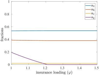
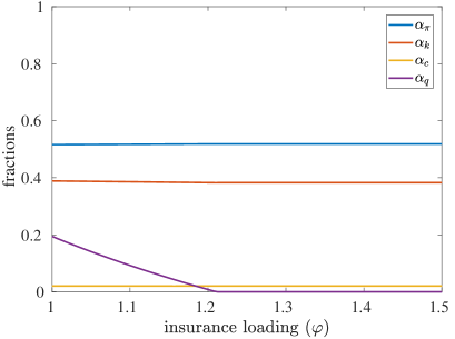
(a)	(b)
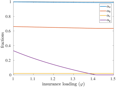
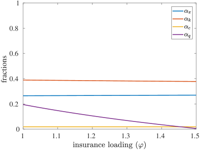
(c)	(d)

Figure 1: Fractions of wealth invested in risky asset, durable good, perishable good and insurance coverage purchase as a function of the insurance loading factor under different scenarios: (a) base scenario; (b) negative jumps of risky asset prices; (c) negative correlation between risky asset and durable good prices and (d) higher risk aversion.

4 Solution with transaction costs on the durable good

In this section we consider the optimal consumption, asset allocation and insurance coverage strategy for an economic agent who faces positive transaction costs proportional to the sale price of durable good, assuming that to change allocation into durable good one has to sell the whole good and buy a new one, e.g., a house. We assume the transaction cost is proportional to the total value of the durable good just before transaction, with a proportionality factor $\theta>0$.

With transaction costs, we cannot find an semi-explicit solution for the economic agent’s optimal dicesion problem. Instead we seek numerical solution of this problem. According to Damgaard et al. (2003) fixed transaction costs implies that the durable good will be traded at most a countable number of times. In particular, at any moment, the agent decides on the rate of consumption, holding positions of the risky asset as well as the level of insurance coverage to purchase. Moreover, the agents decides whether or not to trade the durable good, and if so, the holding position of the durable good after trading, based on all current information. Evidently, the agent’s optimization problem is in the form of a combined stochastic and impulse control problem.

Given the transaction cost of trading the durable good, the solvency region for the state variables becomes $\{(x,k,p):\,x>\theta kp,k\geq 0,p\geq 0\}$. In other words, the agent must be solvent after immediate liquidation of all assets with liquidation costs deducted. The solvency condition (2.7) is modified as

$$\begin{cases}X(t_{-})-\eta\pi_{1}(t_{-})>\theta K(t)P(t),\\ X(t_{-})-(\ell K(t_{-})P(t)-q(t))>\theta K(t)P(t)\end{cases}$$ (4.1)

for $t>0$. In other words, at any moment, the agent must be able to sell the durable good stock and stay solvent, given that a stock market crash or insurance event may occur.

Similar to the no transaction cost case, the agent’s value function is time-independent. Due to the transaction costs, the value function now depends on the durable good holding $K(0)=k$, where without loss of generality, we assume the current time is $t=0$. The agent must decide when to trade the durable good based on current information. The next time to trade the durable good is thus a stopping time, denoted by $\tau$ with $\tau>0$. For $t\in(0,\tau)$, the durable good stock is given by

$$K(t)=K(0)e^{-\delta t}(1-\ell)^{N_{2}(t)}=K(0)e^{-\xi(t)},$$ (4.2)

where $\xi(t)=\delta t-\log(1-\ell)N_{2}(t)$, due to depreciation of the durable good at the rate $\delta$, and the insurance events causing an $\ell\times 100\%$ percentage loss, with occurances represented by the Poisson process $N_{2}$. Following the principle of dynamic programming, (2.13) is modified as

$$V(x,k,p)= \underset{\left({\tau,K(\tau),{\bm{\pi}}^{(\tau)}}\right)}{\sup}E\Big{(}\int_{0}^{\tau}e^{-\rho t}u\left({c(t),ke^{-\xi(t)}}\right)dt$$ (4.3)

$$+e^{-\rho\tau}V\left({X(\tau_{-})-\theta ke^{-\xi(\tau)}P(\tau),K(\tau),P(\tau)}\right)\Big{)},$$

where $\bm{\pi}^{(\tau)}$ denotes any admissible strategy restricted to $(0,\tau)$ without durable good trading, and $K(\tau)\geq 0$ denotes holding of the durable good immediately after $\tau$. The agent must be solvent after trading the durable good. That is, $X(\tau_{-})-\theta ke^{-\xi(\tau)}P(\tau)>0$.

Before proceeding with the numerical solution to (4.3), we first characterize the optimal value function with the following upper and lower bounds:

$$\frac{\underline{\alpha}}{1-\gamma}p^{-(1-\beta)(1-\gamma)}(x-\theta kp)^{1-\gamma}\leq V(x,k,p)\leq\frac{\bar{\alpha}}{1-\gamma}p^{-(1-\beta)(1-\gamma)}x^{1-\gamma},$$ (4.4)

where $\bar{\alpha}=\alpha_{v}$ is given by (3.4) or (3.5), and $\underline{\alpha}=\frac{\beta^{\beta(1-\gamma)}(1-\beta)^{(1-\beta)(1-\gamma)}r^{\beta(1-\gamma)}}{\rho+(\delta-\ell\lambda_{2})(1-\beta)(1-\gamma)}$. Here the upper bound is given by the value function in the no transaction cost case. The lower bound corresponds to a simple suboptimal strategy outlined in Damgaard et al. (2003) and de Matos and Silva (2014). Moreover, following arguments similar to those in the no transaction cost case, it can be shown that $V(x,k,p)$ is homogenous of degree $(1-\gamma)$ in $(x,k)$ and degree $\beta(1-\gamma)$ in $(x,p)$. By applying this homogeneity, the value function can be reduced as

$$V(x,k,p)=k^{1-\gamma}p^{\beta(1-\gamma)}v\left({\frac{x}{kp}}\right)$$ (4.5)

for all $(x,k,p)$ belonging to the solvency region. Here $v(z)=V(z,1,1)$ and the solvency region in terms of $z=\frac{x}{kp}$ is given by $\{z\geq\theta\}$. If $z=\theta$, or $x=\theta kp$, that is, the agent’s total wealth is just enough to cover the liquidation cost of his/her durable good, the agent must liquidate immediately to avoid insolvency. This implies $v(\theta)=0$. By substituting (4.5) into (4.4), the transformed value function is bounded by

$$\frac{\underline{\alpha}}{1-\gamma}(z-\theta)^{1-\gamma}\leq v(z)\leq\frac{\bar{\alpha}}{1-\gamma}z^{1-\gamma}.$$ (4.6)

By denominating in the durable good value $K(t)P(t)$, the transformed wealth $Z(t)=\frac{X(t)}{K(t)P(t)}$, the transformed rate of perishable consumption $\hat{c}(t)=\frac{c(t)}{K(t)P(t)}$, the transformed insurance coverage $\hat{q}(t)=\frac{q(t)}{K(t)P(t)}$ and the transformed risky asset holding $\hat{\pi}_{1}(t)=\frac{\pi_{1}(t)}{K(t)P(t)}$. In the transformed model the solvency condition (4.1) becomes

$$\begin{cases}Z(t_{-})-\eta\hat{\pi}_{1}(t_{-})>\theta,\\ Z(t_{-})-(\ell-\hat{q}(t))>\theta.\end{cases}$$ (4.7)

By subsituting (4.5) into (4.3) and after some algebra, we obtain the following optimization problem for the transformed value function,

$$p^{\beta(1-\gamma)}v(z)= \underset{\left({\tau,{\hat{\bm{\pi}}}^{(\tau)}}\right)}{\sup}E\Bigg{(}\frac{1}{1-\gamma}\int_{0}^{{\tau}}e^{-{\rho}t-(1-\gamma)\xi(t)}\hat{C}(t)^{\beta(1-\gamma)}P(t)^{\beta(1-\gamma)}dt$$ (4.8)

$$+e^{-{\rho}\tau-(1-\gamma)\xi(\tau)}P({\tau})^{\beta(1-\gamma)}\mathcal{M}v(Z({\tau}_{-}))\Bigg{)},$$

where $\hat{\bm{\pi}}^{(\tau)}$ denotes any admissible strategy in the transformed controls, restricted to $(0,\tau)$, and the intervention value function $\mathcal{M}v(z)$ is given by

$$\mathcal{M}v(Z(\tau_{-}))=(Z(\tau_{-})-\theta)^{1-\gamma}M,$$ (4.9)

where

$$M=\underset{Z(\tau)\geq\theta}{\sup}Z(\tau)^{\gamma-1}v(Z(\tau)).$$ (4.10)

Here $\mathcal{M}$ is the so-called intervention operator that maps the value function $v$ to the (optimal) intervention value function $\mathcal{M}v$, by selecting the optimal control $Z(\tau)$ that maximizes the latter. In other words, the intervention value function $\mathcal{M}v(Z(\tau_{-}))$ represents the value received by the agent by trading the durable good immediately and optimally, given current transformed wealth $Z(\tau_{-})$. Here $Z(\tau)$ is determined by $K(\tau)$, holding of the durable good after trading, through $Z(\tau)=\frac{ke^{-\xi(\tau)}(Z(\tau_{-})-\theta)}{K(\tau)}$. Denoting by $z^{\ast}=\arg\max_{z\geq\theta}z^{\gamma-1}v(z)$, the optimal durable good stock immediately after a transaction is thus given by

$$K^{*}(\tau)=\frac{ke^{-\xi(\tau)}(Z(\tau_{-})-\theta)}{z^{*}}.$$ (4.11)

Applying Ito’s formula to (4.8), we obtain the HJB equation as

$$0=\max\Big{\{}H(z,v,v^{\prime},v^{\prime\prime}),\mathcal{M}v(z)-v(z)\Big{\}},$$ (4.12)

where the HJB operator

$$H(z,v,v^{\prime},v^{\prime\prime})=\underset{(\hat{\pi}_{1},\hat{c},\hat{q})}{\sup}\Big{\{}-\bar{\rho}v(z)+\mathcal{L}^{(\hat{\pi}_{1},\hat{c},\hat{q})}v(z)+\frac{\hat{c}^{\bar{\beta}}}{1-\gamma}\Big{\}}$$ (4.13)

with $\bar{\beta}=\beta(1-\gamma)$, and the generator

$$\mathcal{L}^{(\hat{\pi}_{1},\hat{c},\hat{q})} v(z)=v(z)\big{(}\bar{\beta}\mu_{P}-\frac{1}{2}\bar{\beta}(1-\bar{\beta})\sigma^{2}_{P}\big{)}$$ (4.14)

$$+ v^{\prime}(z)\big{(}(1-z)(\bar{\mu}_{P}-(1-\bar{\beta})\sigma_{P}^{2})+\hat{\pi}_{1}(\bar{\mu}_{S}-(1-\bar{\beta})\sigma_{S}\sigma_{P_{1}})-\hat{c}-\lambda_{2}\varphi\hat{q}\big{)}$$

$$+ \frac{1}{2}v^{\prime\prime}(z)\big{(}((1-z)\sigma_{P_{1}}+\hat{\pi}_{1}\sigma_{S})^{2}+(1-z)^{2}\sigma_{P_{2}}^{2}\big{)}$$

$$+ \lambda_{1}\big{(}v(z-\eta\hat{\pi}_{1})-v(z)\big{)}+\lambda_{2}\big{(}(1-\ell)^{1-\gamma}v(\frac{z-\ell+\hat{q}}{1-\ell})-v(z)\big{)},$$

where $\bar{\rho}=\rho+\delta(1-\gamma)$, $\bar{\mu}_{P}=\mu_{P}-r-\delta$, $\bar{\mu}_{S}=\mu_{S}+\lambda_{1}\eta-r$, $\sigma_{P}^{2}=\sigma_{P_{1}}^{2}+\sigma_{P_{2}}^{2}$.

The HJB equation in the form of (4.12) together with suitable boundary conditions is denoted by Seydel (2010) as the HJB quasi-variational inequality (HJBQVI), where the solution is formuated under the framework of viscosity solutions. Existence and uniqueness of the viscosity solution to the above HJBQVI is unfortunately beyond the scope of this paper. Interested readers are referred to Seydel (2010) and references therein for related concepts and proofs of existence and uniqueness of the viscosity solution to the HJBQVI associated with a class of combined stochastic and impulse control problems with jump-diffusion models, of which the current model is a special case. We assume the model parameters are such that a unique viscosity solution to (4.12) exists in the sense of Seydel (2010). In particular, we assume as in the case without transaction costs that the agent’s time preference parameter $\rho$ is large enough to guarantee the so-called transversality condition, given by

$$\bar{\rho}\geq\bar{\beta}\mu_{P}-\frac{1}{2}\bar{\beta}(1-\bar{\beta})\sigma^{2}_{P},$$ (4.15)

is satisfied. See Dammgard (2003) for a similar condition under a slightly different model setting.

5 Numerical Solutions

The HJB equations (4.12)$\sim$(4.14) may be recast into the standard form of a complimentarity problem as

$$\begin{cases}-\bar{\rho}v(z)+\mathcal{L}^{(\hat{\pi}^{*}_{1},\hat{c}^{*},\hat{q}^{*})}v(z)+\frac{\hat{c}^{*\bar{\beta}}}{1-\gamma}\leq 0,\\ \mathcal{M}v(z)-v(z)\leq 0,\\ \bigg{(}-\bar{\rho}v(z)+\mathcal{L}^{(\hat{\pi}^{*}_{1},\hat{c}^{*},\hat{q}^{*})}v(z)+\frac{\hat{c}^{*\bar{\beta}}}{1-\gamma}\bigg{)}\bigg{(}\mathcal{M}v(z)-v(z)\bigg{)}=0,\end{cases}$$ (5.1)

where ${M}v$ is given by (4.9), and $(\hat{\pi}^{*}_{1},\hat{c}^{*},\hat{q}^{*})$ are obtained by maximizing (4.13). The system (5.1) is in the form of an implicit nonlinear complimentarity problem (NLCP) with both $\mathcal{L}$ and $\mathcal{M}v$ depending on the unknown function $v$. Solution to (5.1) can be obtained by the stopping time iteration procedure proposed by Seydel (2010) as is outlined below. See also Chancelier et al. (2002).

The value function may first be initialized by considering sub-optimal strategies that never trade the durable good. The sub-optimal value function is obtained by solving the HJB equation

$$-\bar{\rho}v(z)+\mathcal{L}^{(\hat{\pi}^{*}_{1},\hat{c}^{*},\hat{q}^{*})}v(z)+\frac{\hat{c}^{*\bar{\beta}}}{1-\gamma}=0,$$ (5.2)

with only the stochastic controls. By solving (5.2) numerically, we obtain the first suboptimal estimation $v_{0}$ of the value function. Assuming the current estimation $v_{n}$ is obtained, we solve the explicit NLCP (5.1) with the unknown intervention value function $\mathcal{M}v$ replaced by the current estimation $\mathcal{M}v_{n}$, leading to the next value function estimation $v_{n+1}$. This procedure may be continued until convergence. This consists the “main loop” of the solution algorithm. Note that $v_{n}$ represents the value function when the agent is allowed to trade the durable good at $n$ future stopping times. As more tradings of the durable good are allowed, the value function improves, so that $v_{n+1}\geq v_{n}$. The sequence of suboptimal value functions $(v_{n})$ converges to $v$ monotonically as $n\rightarrow\infty$. The main loop is outlined in Algorithm 1.

Algorithm 1 The main loop

1:set $n=0$, solve (5.2) for $v_{n}$

2:set error bound $e_{m}>0$

3:while true do

4:   compute $\mathcal{M}v_{n}$ and set ${\mathcal{M}v}=\mathcal{M}v_{n}$ in (5.1)

5:   solve the NLCP (5.1) for $v_{n+1}$ using Algorithm 2

6:   if $\|v_{n+1}-v_{n}\|_{\infty}<e_{m}$ then

7:      break

8:   end if

9:   set $n=n+1$

10:end while

11:return $v_{n}$

Solution to the explicit NLCP, i.e., the “inner loop”, may be obtained by iteratively solving a sequence of linear complimentarity problems (LCPs). In particular, given the current estimation $v_{n}$, the optimal stochastic controls $\hat{\pi}^{*}_{1},\hat{c}^{*},\hat{q}^{*}$ may be obtained by maximizing (4.13), leading to an explicit generator $\mathcal{L}$. This may be substituted into (5.1), leading to an LCP. By solving the LCP numerically, the current estimation $v_{n}$ is updated, and is used to update the stochastic controls by maximizing (4.13). This iteration is carried out until convergence of $v_{n}$. The inner loop is outlined in Algorithm 2.

Algorithm 2 The inner loop

1:set erorr bound $e_{i}>0$

2:set $v=u=\max(\mathcal{M}v_{n},v_{n})$

3:while true do

4:   set $v_{\rm last}=v$

5:   solve for $\hat{\pi}^{*}_{1},\hat{c}^{*},\hat{q}^{*}$ from (4.13) with $v_{\rm last}$

6:   compute the discrete version $L$ of $\mathcal{L}^{(\hat{\pi}^{*}_{1},\hat{c}^{*},\hat{q}^{*})}$

7:   solve the resulting LCP (5.3) for $v$ using Algorithm 3

8:   if $\|v-v_{\rm last}\|_{\infty}<e_{i}$ then

9:      break

10:   end if

11:end while

12:return $v$

The discrete LCP problem may be solved using the projected successive over relaxation (PSOR) procedure proposed by Cryer (1971). See also Hackbusch (1994); Hilber et al. (2013). To solve the LCP using PSOR, we discretize $v$ on a regular numerical grid using a suitable discrete scheme, leading to the discrete LCP

$$\begin{cases}\bar{\rho}v-Lv-\frac{\hat{c}^{*\bar{\beta}}}{1-\gamma}\geq 0,\\ v-u\geq 0,\\ \bigg{(}\bar{\rho}v-Lv-\frac{\hat{c}^{*\bar{\beta}}}{1-\gamma}\bigg{)}\cdot\bigg{(}v-u\bigg{)}=0,\end{cases}$$ (5.3)

where $L$ is the matrix obtained by discretizing the generator $\mathcal{L}^{(\hat{\pi}^{*}_{1},\hat{c}^{*},\hat{q}^{*})}$ with current controls, $\hat{c}^{*}$ is the current consumption vector, $v$ is the unknown value function vector, and $u=\max\left({\mathcal{M}v,v}\right)$ is the improved intervention value vector, where a discrete intervention operator $\mathcal{M}$ is understood. This leads to an equivalent iteration with faster convergence for the PSOR. To present the PSOR procedure, we rewrite (5.3) in the general form as

$$\begin{cases}Av-b\geq 0,\\ v-u\geq 0,\\ \big{(}Av-b\big{)}^{\top}\big{(}v-u\big{)}=0.\end{cases}$$ (5.4)

The PSOR procedure we adopt is outlined in Hilber et al. (2013), Table 5.1, which is reproduced as Algorithm 3, where $0<\omega<2$ is the relaxation parameter, and $k=1,...,K$ is the spatial index for $z$.

Algorithm 3 The PSOR iteration

1:set erorr bound $e_{p}>0$

2:while true do

3:   set $v_{\rm last}=v$

4:   for $k=1,...,K$ do

5:      $w(k)=v(k)+\frac{\omega}{A(k,k)}\left({b(k)-\sum_{j}A(k,j)v(j)}\right)$

6:      $v(k)=\max\left({w(k),u(k)}\right)$

7:   end for

8:   if $\|v-v_{\rm last}\|_{\infty}<e_{p}$ then

9:      break

10:   end if

11:end while

12:return $v$

It should be noted that in order for the afore-mentioned solution algorithm to converge, a suitable discretization scheme must be adopted. Here we adopt a finite difference (FD) discretization scheme suggested by Barles and Souganidis (1991). The reader is referred to Barles and Souganidis (1991) for detailed analysis including convergence results of the proposed discrete scheme.

To test our numerical algorithms, we conduct a number of numerical experiments using parameters listed in Table 2. The value function, intervention value function and associated no-trading zone, etc., for the case $\varphi=1.2$ are shown in Figure 2. The bounded monotone convergence of the value function with an increasing number of stopping time iterations is shown in Figure 2 (a), and Figure 2 (b) shows the convergence of the corresponding $M$ value, given by (4.10). The value functions and in particular, the excess value function $v-\mathcal{M}v$, supported on the no-trading zone, are shown in Figure 2 (c) and (d). Evidently the no-trading zone is characterized by an upper and lower bound in the transformed state variable $z$. Within the no-trading zone, the agent enjoys more value than trading the durable good immediately and optimally, that is, the optimal intervention value. Outside the no-trading zone, the optimal intervention value exceeds the value of no trading, thus trade happens immediately to bring the value function back to the optimal position within the no-trading zone, that is, the position that maximizes the value function within the no-trading zone. Afterwards, the agent does not trade the durable good until the transformed state variable drifts or jumps outside the no-trading zone.

To investigate the effects of changing the insurance loading factor $\varphi$, we additionally take $\varphi=1.0\sim 1.5$, with an increment of $0.1$. Figure 3 demonstrates the change of the $M$ value, the excess value function and the no-trading zone with the increment of $\varphi$. It can be seen that the excess value function decreases, and the no-trading zone shifts to the right with increasing insurance loading. The shift of the no-trading zone is due to reduced durable good holding with increasing insurance cost, and an inversely proportional relation between the durable good holding $k$ and the transformed state variable $z$. The decrement of the excess value functions is due to overall decrement of the value function with increased cost.

Table 2: Parameters used in the numerical experiments

$\beta$	0.5		$\gamma$	0.9		$r$	0.02
$\mu_{S}$	0.06		$\sigma_{S}$	0.25		$\mu_{P}$	0.02
$\delta$	0.015		$\sigma_{P_{1}}$	0.1		$\sigma_{P_{2}}$	0.2
$\eta$	0.1		$\lambda_{1}$	0		$\ell$	0.5
$\lambda_{2}$	0.01		$\rho$	0.04		$\theta$	0.05

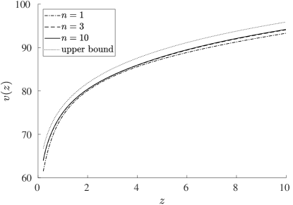
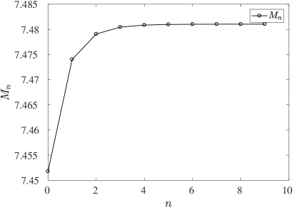
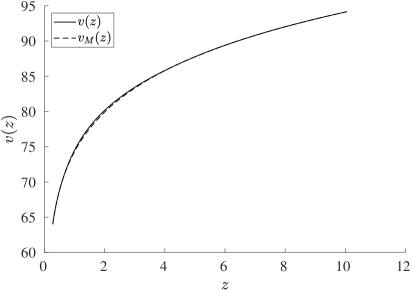
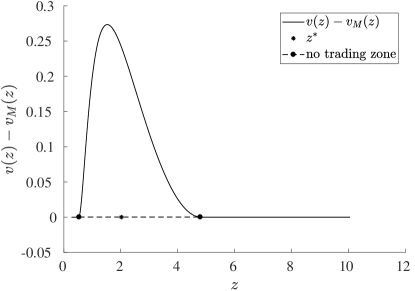
(a) convergence of the value function (b) convergence of the $M$ value (c) value and intervention value functions (d) excess value function

Figure 2: Value function $v(z)$, excess value function $v(z)-v_{M}(z)$, where $M=\mathcal{M}(v)$, no-trading zone, and optimal durable good holding level $z^{*}$ for insurance loading $\varphi=1.2$.

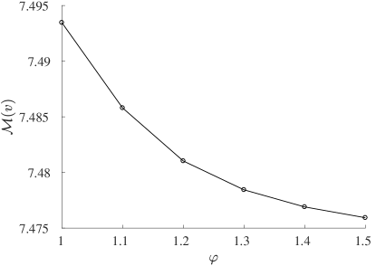
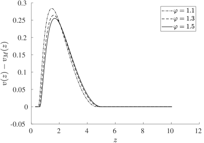
(a) intervention value change with $\varphi$ (b) excess value function change with $\varphi$

Figure 3: The effect of changing insurance loading $\varphi$: Panel (a) shows the intervention value $\mathcal{M}(v)$ as a function of $\varphi$; Panel (b) shows the excess value function $v(z)-v_{M}(z)$, where $M={\mathcal{M}(v)}$ for different values of $\varphi$.

6 Summary

In this paper we considered an economic agent’s optimal consumption and investment problem with an infinite time horizon in a continuous-time economy. The agent is faced with multiple risk factors including equity market risks and crashes, durable good price fluctuations and insurable events that cause damage to the durable good, and must make multiple decisions including risky and riskless asset allocations, perishable and durable goods consumptions, and optional insurance coverage for the durable good. The agent derives utilities from consumptions over an infinite time horizon, in the form of expected utility of a CRRA type utility function. We first devised a semi-explicit solution for the optimal decision problem when no transaction costs are present. We demonstrate that an increase in premium loading decreases the demand for the durable good and their insurance coverage.

We next considered the optimal decision problem when transaction costs are charged for trading the durable good proportional to the total value of the durable good being traded. We formulate the agent’s optimal decision problem as a combined stochastic and impulse control problem, with an implicit intervention value function. The problem falls into the category of the so-called HJBQVI. To solve the HJBQVI, we follow the numerical solution procedure known as stopping time iteration, and numerically obtains the agent’s optimal value function. Once implemented correctly, the optimal value function follows a bounded monotone convergence. Moreover, the numerical procedure automatically identifies the so-called no-trading zone in a nonparametric fashion. Within the no-trading zone, the optimal agent does not trade the durable good. Once the state variables move outside the no trading zone, the agent trades the durable good optimally to bring the state variables back to the optimal position within the no-trading zone. We further investigated numerically the effect of insurance costs to the optimal value function.

References

- Arrow (1971) Arrow, K. J., 1971. The theory of risk aversion. In: Arrow, K. J. (Ed.), Essays in the theory of risk-bearing. Markham Chicago, pp. 90–120.
- Barles and Souganidis (1991) Barles, G., Souganidis, P. E., 1991. Convergence of approximation schemes for fully nonlinear second order equations. Asymptotic Analysis 4 (3), 271–283.
- Briys (1986) Briys, E., 1986. Insurance and consumption: The continuous time case. The Journal of Risk and Insurance 53 (4), 718–723.
- Chancelier et al. (2002) Chancelier, J.-P., Øksendal, B., Sulem, A., 2002. Combined stochastic control and optimal stopping, and application to numerical approximation of combined stochastic and impulse control. Proceedings of the Steklov Institute of Mathematics 237, 140–163.
- Cocco (2004) Cocco, J. F., 2004. Portfolio choice in the presence of housing. The Review of Financial Studies 18 (2), 535–567.
- Cryer (1971) Cryer, C. W., 1971. The solution of a quadratic programming problem using systematic overrelaxation. SIAM Journal on Control 9 (3), 385–392.
- Cuoco and Liu (2000) Cuoco, D., Liu, H., 2000. Optimal consumption of a divisible durable good. Journal of Economic Dynamics and Control 24 (4), 561–613.
- Damgaard et al. (2003) Damgaard, A., Fuglsbjerg, B., Munk, C., 2003. Optimal consumption and investment strategies with a perishable and an indivisible durable consumption good. Journal of Economic Dynamics and Control 28 (2), 209–253.
- de Matos and Silva (2014) de Matos, J. A., Silva, N., 2014. Consuming durable goods when stock markets jump: A strategic asset allocation approach. Journal of Economic Dynamics and Control 42, 86–104.
- Detemple and Giannikos (1996) Detemple, J. B., Giannikos, C. I., 1996. Asset and commodity prices with multi-attribute durable goods. Journal of Economic Dynamics and Control 20 (8), 1451–1504.
- Gollier (1994) Gollier, C., 1994. Insurance and precautionary capital accumulation in a continuous-time model. Journal of Risk and Insurance 61 (1), 78–95.
- Gollier and Schlesinger (1995) Gollier, C., Schlesinger, H., 1995. Second-best insurance contract design in an incomplete market. The Scandinavian Journal of Economics 97 (1), 123–135.
- Hackbusch (1994) Hackbusch, W., 1994. Iterative solution of large sparse systems of equations. Vol. 95. Springer.
- Hilber et al. (2013) Hilber, N., Reichmann, O., Schwab, C., Winter, C., 2013. Computational Methods for Quantitative Finance. Springer.
- Hindy and Huang (1993) Hindy, A., Huang, C., 1993. Optimal consumption and portfolio rules with durability and local substitution. Econometrica: Journal of the Econometric Society 61 (1), 85–121.
- Moore and Young (2006) Moore, K. S., Young, V. R., 2006. Optimal insurance in a continuous-time model. Insurance: Mathematics and Economics 39 (1), 47–68.
- Mossion (1968) Mossion, J., 1968. Optimal multiperiod portfolio policies. The Journal of Business 41 (2), 215–229.
- Perera (2010) Perera, R. S., 2010. Optimal consumption, investment and insurance with insurable risk for an investor in a lévy market. Insurance: Mathematics and Economics 46 (3), 479–484.
- Seydel (2010) Seydel, R. C., 2010. Impulse control for jump-diffusions: Viscosity solutions of quasi-variational inequalities and applications in bank risk management. Ph.D. thesis, Verlag nicht ermittelbar.
- Touzi (2000) Touzi, N., 2000. Optimal insurance demand under marked point processes shocks. Annals of Applied Probability 10 (1), 283–312.