Lens Model and Source Reconstruction Reveal the Morphology and Star Formation Distribution in the Cool Spiral LIRG SGAS J143845.1$+$145407

Abstract

We present Hubble Space Telescope (HST) imaging and grism spectroscopy of a strongly lensed LIRG at $z=0.816$, SGAS 143845.1$+$145407, and use the magnification boost of gravitational lensing to study the distribution of star formation throughout this galaxy. Based on the HST imaging data, we create a lens model for this system; we compute the mass distribution and magnification map of the $z=0.237$ foreground lens. We find that the magnification of the lensed galaxy ranges between 2 and 10, with a total magnification (measured over all the images of the source) of $\mu$=$11.8^{+4.6}_{-2.4}$. We find that the total projected mass density within $\sim 34$ kpc of the brightest cluster galaxy is $6.0^{+0.3}_{-0.7}\times 10^{12}$ M_⊙. Using the lens model we create a source reconstruction for SGAS 143845.1$+$145407, which paired with a faint detection of H$\alpha$ in the grism spectroscopy, allows us to finally comment directly on the distribution of star formation in a $z\sim 1$ LIRG. We find widespread star formation across this galaxy, in agreement with the current understanding of these objects. However, we note a deficit of H$\alpha$ emission in the nucleus of SGAS 143845.1$+$145407, likely due to dust extinction.

1. Introduction

Observations of luminous infrared galaxies (LIRGs, galaxies with total infrared luminosity (8-1000 $\mu$m) of $10^{11-12}L_{\odot}$ and a star formation rate (SFR) of $\mathtt{\sim}10-100\,M_{\odot}\ \text{yr}^{-1}$), which dominate star formation at $z\sim 1$, indicate that they evolve strongly with redshift.

Spectroscopy and spectral energy distribution (SED) measurements of LIRGs indicate that at $z=0$ they are more likely to have warmer SEDs than their $z\sim 1$ counterparts (Rowan-Robinson et al., 2004), and that the temperature of the dust-reprocessed infrared radiation gets colder with increasing redshift (Rowan-Robinson et al. 2005; Sajina et al. 2006; Symeonidis et al. 2009; Elbaz et al., 2010; Hwang et al., 2010). Several studies (e.g., Papovich et al., 2007; Rigby et al., 2008; Farrah et al., 2008; Menéndez-Delmestre et al., 2009) show that the strength of the polycyclic aromatic hydrocarbon features increase with redshift for galaxies with constant luminosity. Morphologically, radio and submm interferometry show that the spatial extent of star formation in LIRGs and ULIRGs (ultraluminous infrared galaxies–those with total infrared luminosity $>10^{12}L_{\odot}$ and a SFR exceeding $\mathtt{\sim}100M_{\odot}\ \text{yr}^{-1}$) is considerably larger at $0.4<z<2.5$ than in the local universe (Rujopakarn et al. 2011).

These multiple lines of evidence therefore indicate that the mode of star formation in LIRGs evolves significantly with redshift: At $z=0$, star formation occurs on sub-galactic scales of hundreds of parsecs at most, resulting in hot infrared SEDs and weak aromatic features, while star formation at higher redshifts is dominated by low SFRs in galaxy-wide bursts, resulting in cooler SEDs and stronger aromatic features.

However, existing direct imaging studies lack the resolution required to distinguish between these two star formation morphologies at high redshift. At $z>0.4$, galaxies are unresolved by Spitzer and Herschel, for example, and even with interferometry in the radio and submm, a beam size of $0\farcs 3-0\farcs 5$ is only a few times smaller than the size of the sources, making it impossible to robustly test whether the distribution of star formation is different in $z\sim 1$ LIRGs than it is in those at $z\sim 0$.

This spatial resolution limitation can be overcome if we are able to take advantage of the magnifying power of gravitational lensing. When paired with the already-high resolution of telescopes like the Hubble Space Telescope (HST), gravitational lensing enables observations on scales 10-100 times smaller than otherwise possible, providing insights into the detailed physical properties of high redshift galaxies (e.g., Wuyts et al. 2012; Bayliss et al. 2014; Bordoloi et al. 2016). In fact, using gravitational lensing, Johnson et al. (2017a) recently measured the sizes of individual star forming regions in a galaxy at $z=2.49$ and found some as small as 40 parsecs across, demonstrating the importance of this magnification boost to studying the details of star formation in high redshift galaxies. This means that in order to directly determine whether the mode of star formation in LIRGs really does evolve between $z=1$ and $z=0$, the ideal target to observe would be a strongly lensed galaxy at $z\sim 1$ with properties typical of LIRGs at that redshift.

SGAS J143845.1$+$145407 is such an object. First reported by Gladders et al. (2013), SGAS J143845.1$+$145407 (hereafter SGAS J1438) is a bright lensed galaxy behind the lensing cluster SDSS J1438$+$1454 (Figure 1). Using photometry in 18 bands from the blue optical to $500\ \mu m$, and optical and near infrared spectroscopy, these authors determined that SGAS J1438 is a cool LIRG undergoing dusty star formation. Other than being highly magnified, SGAS J1438 is intrinsically a typical LIRG at $z=0.816$.

We take advantage of this unique opportunity to study the details of star formation in a prototypical high-redshift LIRG. We present new HST imaging data of SDSS J1438$+$1454 in § 2 and a lens model based on new constraints from these data in § 3. We discuss the implications of this lens model in § 4. Using the lens model we produce a source plane reconstruction of SGAS J1438 in § 5, which we pair with HST grism spectroscopy data in § 6 to constrain the spatial extent of star formation in this $z=0.816$ LIRG. This allows us to directly test the current understanding of the evolution of star formation in LIRGs from $z=1$ to $z=0$.

Where necessary, we assume a flat cosmology with $\Omega_{\Lambda}=0.7$, $\Omega_{m}=0.3$, and $H_{0}=70$ km s^-1 Mpc^-1. In this cosmology $1\arcsec$ corresponds to $3.758$ kpc at the cluster redshift, $z=$0.237, and $7.559$ kpc at the source redshift, $z=$0.816. Magnitudes are reported in the AB system.

2. Data

SDSS J1438$+$1454 was observed by HST Cycle 21 program GO13437 (PI: Rigby) during three orbits. Imaging with the Advanced Camera for Surveys (ACS) was executed over one orbit on GMT 2014 March 5, in F814W (600 s) and F606W (780 s). Wide Field Camera 3 (WFC3) grism spectroscopy was conducted in two different roll angles, one on GMT 2014 March 5 and one on GMT 2014 May 30, using the G141 grism (2406 s each). F140W imaging frame was taken at each roll angle (285 s each), giving a total imaging time in this band of 570 s. The ACS images were taken with a 3-point line dither using a 1000$\times$1000 pixel subraster to manage buffer dumps, resulting in three frames per filter. Since the charge transfer efficiency (CTE) of the ACS detector is decreasing, post-observation image corrections were applied to individual exposures using the pixel-based empirical CTE correction software provided by Space Telescope Science Institute (STScI). Individual frames were then combined using AstroDrizzle (Gonzaga at al. 2012) with a pixel scale of $0\farcs 03$ pixel^-1, and a drop size of 0.5 (WFC3) and 0.8 (ACS), following Sharon et al. (2014). All the images were aligned and registered to the same pixel frame as the F140W image.

The slitless spectroscopy data were reduced using the Grizli pipeline. Each visit was processed separately rather than being stacked because the data were taken with different roll angles. The two-dimensional spectra of each of the four images of SGAS J1438 are significantly contaminated by light from the brightest cluster galaxy (BCG) and other bright galaxies. To minimize the effects of the light from these objects we deviate from the standard Grizli procedure by modeling the contamination from the galaxies that directly affect the spectra of SGAS J1438 separately from the rest of the field, using GALFIT (Peng et al. 2002, 2014). We find that for the purpose of assigning light to individual objects in areas where light from multiple galaxies overlaps, the GALFIT modeling is better than the Source Extractor segmentation maps that are part of the standard Grizli pipeline. Because of this we use the following alternative method (G. Brammer, private communication): We truncate the GALFIT models when the flux from an object falls to less than 0.001 of the flux of the central pixel. The GALFIT models were then subtracted from the direct images, and the initial contamination models were computed for the remaining objects. The initial contamination models for the two sets of galaxies were combined before the final refinement of the models was conducted. This two-part modeling process resulted in two-dimensional spectral extractions with substantially less contamination from bright nearby galaxies than the standard Grizli pipeline. However, as we will discuss in § 6, contamination was still significant.

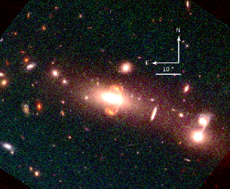
Figure 1.— Composite color HST image of SDSS J1438+1454 in F140W (red), F814W (green) and F606W (blue). The HST imaging data are consistent with this being a low-mass cluster, dominated by the BCG and a few cluster member galaxies. In these data two of the multiple images of SGAS J1438 are easily identified north and south of the BCG. There are also two partial images that lie to the east and west of the BCG, but they are obscured by the intracluster light.

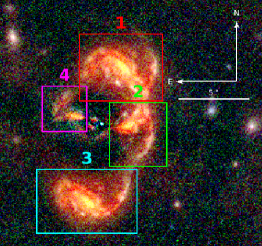
Figure 2.— A zoom-in view of SGAS J1438; the light of the BCG was modeled with GALFIT (Peng et al. 2002, 2014) and subtracted from the imaging data. The filters are the same as in Figure 1. We mark each of the unique images of SGAS J1438 with boxes. Images 1 and 3 (red and cyan boxes, respectively) are of the same parity and approximately the same magnification. Images 2 and 4 (green and magenta boxes, respectively) are partial images. We note a residual unresolved blue clump close to the center of the BGC that is probably due to emission in the lens galaxy and not to lensing.

3. Strong Lens Model

To analyze the images of the lensed galaxy we model the light of the foreground BCG with a multi-component Sérsic profile using GALFIT, and subtract the model from the imaging data in each band. The result (Figure 2) reveals the images of the lensed galaxy that are buried in the light of the foreground BCG.

The high resolution HST data confirm the lensing interpretation of Gladders et al. (2013), which was based on lower-resolution imaging in 18 bands, spanning 0.5 to 500 $\mu m$, from Gemini, Magellan, Spitzer Space Telescope, Wide-field Infrared Survey Explorer (WISE), and the Herschel Space Observatory. The strong lensing potential of the foreground cluster causes the appearance of four images of SGAS J1438. Two of these are complete images appearing to the north and south of the BCG (labeled 1 and 3 in Figure 2, respectively); and two are partial images appearing west and east of the BCG (labeled 2 and 4, respectively). In each of the images we identify a number of distinct emission knots, most prominent in F606W and F814W.

We matched the multiply-imaged knots between instances of the lensed galaxy by considering the location of the knots within the galaxy, lensing parity, color, magnification, and brightness. Several emission knots are easily distinguishable, and thus are used to constrain the lens model (Figure 3). Including the bulge of the galaxy, a total of $38$ emission knots were used as positional constraints. Table 1 lists the IDs and coordinates of the emission knots that were used in the lens model.

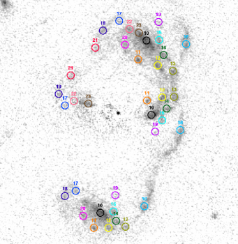
Figure 3.— The emission knots in SGAS J1438 that were used to constrain the lens model are labeled over the F814W image. See also Table 1.

The strong lens model was computed with the public software Lenstool (Jullo et al. 2007), which uses a Bayesian Markov Chain Monte Carlo (MCMC) method to explore the parameter space. The final minimization was done in the image plane by requiring the smallest scatter between the predicted and observed positions of images of each emission knot. We modeled the lens plane as a linear combination of several halos, representing the cluster, the BCG, and cluster-member galaxies. Each halo is parameterized as a pseudo isothermal ellipsoidal mass distribution (PIEMD; Jullo et al. 2007), with the following parameters: position $x$, $y$; ellipticity $e\equiv(a^{2}-b^{2})(a^{2}+b^{2})^{-1}$, where $a$ and $b$ are the semi-major and semi-minor axes, respectively; position angle $\theta$; core and cut radii $r_{core}$ and $r_{cut}$, respectively; and velocity dispersion $\sigma$. All the parameters of the cluster halo were allowed to vary with the exception of the cut radius, which cannot be constrained by the strong lensing evidence and was therefore fixed at $r_{cut}$=1000 kpc. We verify that this assumption does not affect the results of this work. In addition to the cluster halo we placed a halo that represents the central galaxy; its position was fixed on its observed coordinates, its cut radius was fixed at $r_{cut}$=20 kpc, and all other parameters were left free.

Cluster-member galaxies were identified from the HST photometry by their F814W-F140W color in a color-magnitude diagram (Gladders et al. (2000)). The positions, ellipticities, and position angles of each galaxy were fixed to their observed values, and the PIEMD profile parameters were scaled to their F140W luminosity using scaling relations, following Limousin et al. (2005).

Our model is in general agreement with that of Gladders et al. (2013). In particular, we find that the position angle, core radius, and velocity dispersions of the cluster and of the BCG are within the statistical uncertainties of the respective models. We note, however, that due to the smaller number of lensing constraints that were available to Gladders et al. (2013), they had simplified their lens model by stronger assumptions on the extent to which the mass distribution follows the light distribution. They limit the center of the cluster to not be further than $8\farcs 01^{+2.01}_{-3.90}$ from the BCG, in agreement with our findings of $4\farcs 88$. The best-fit model has an image plane rms scatter of $0\farcs 07$. Table 1 lists the rms of each image.

Table 1Lensing Constraints

Image ID	R.A.(J2000)	Decl.(J2000)	rms (′′)	$\left|\mu\right|$
10.1	219.68704	14.904572	0.05	3.2${}_{-0.7}^{+0.6}$
10.2	219.68696	14.903430	0.04	1.8${}_{-0.4}^{+1.6}$
10.3	219.68777	14.901929	0.04	2.4${}_{-0.5}^{+0.4}$
11.1	219.68717	14.904282	0.03	5.4${}_{-1.0}^{+2.4}$
11.2	219.68703	14.903652	0.11	2.8${}_{-0.5}^{+2.5}$
11.3	219.68787	14.901701	0.07	2.1${}_{-0.4}^{+0.2}$
12.1	219.68686	14.904191	0.01	6.4${}_{-1.8}^{+2.0}$
12.2	219.68679	14.903699	0.09	4.5${}_{-0.8}^{+2.5}$
12.3	219.68764	14.901701	0.06	2.2${}_{-0.4}^{+0.2}$
13.1	219.68662	14.904108	0.05	8.0${}_{-2.9}^{+1.4}$
13.2	219.68660	14.903708	0.05	6.4${}_{-0.8}^{+3.2}$
13.3	219.68737	14.901716	0.05	2.3${}_{-0.5}^{+0.2}$
14.1	219.68677	14.904353	0.02	4.2${}_{-1.1}^{+0.8}$
14.2	219.68672	14.903530	0.04	2.9${}_{-0.8}^{+1.5}$
14.3	219.68752	14.901806	0.02	2.4${}_{-0.5}^{+0.3}$
15.1	219.68684	14.904579	0.04	3.1${}_{-0.7}^{+0.5}$
15.2	219.68679	14.903349	0.08	2.1${}_{-0.6}^{+1.1}$
15.3	219.68756	14.901952	0.06	2.6${}_{-0.6}^{+0.4}$
16.1	219.68641	14.904516	0.03	3.1${}_{-0.8}^{+0.2}$
16.2	219.68650	14.903197	0.02	2.9${}_{-1.2}^{+0.6}$
16.3	219.68707	14.902029	0.05	3.1${}_{-0.8}^{+0.5}$
17.1	219.68747	14.904875	0.08	2.7${}_{-0.5}^{+0.4}$
17.3	219.68816	14.902269	0.06	2.9${}_{-0.6}^{+0.7}$
17.4	219.68833	14.903578	0.04	1.7${}_{-0.2}^{+1.4}$
18.1	219.68773	14.904724	0.14	3.3${}_{-0.7}^{+0.8}$
18.3	219.68833	14.902189	0.07	2.6${}_{-0.5}^{+0.5}$
18.4	219.68843	14.903754	0.02	2.1${}_{-0.4}^{+1.3}$
19.1	219.68685	14.904857	0.06	2.5${}_{-0.5}^{+0.3}$
19.2	219.68690	14.903173	0.06	2.1${}_{-0.5}^{+1.2}$
19.3	219.68753	14.902201	0.04	3.2${}_{-0.8}^{+0.9}$
20.1	219.68738	14.904508	0.02	3.8${}_{-0.7}^{+1.3}$
20.3	219.68804	14.901883	0.02	2.3${}_{-0.5}^{+0.4}$
21.1	219.68785	14.904465	0.08	5.6${}_{-1.1}^{+2.7}$
21.4	219.68824	14.904039	0.06	4.6${}_{-1.1}^{+1.7}$
22.1	219.68731	14.904751	0.03	2.9${}_{-0.6}^{+0.6}$
22.4	219.68819	14.903645	0.02	1.4${}_{-0.1}^{+1.7}$
23.1	219.68716	14.904693	0.18	3.0${}_{-0.6}^{+0.5}$
23.4	219.68796	14.903606	0.16	1.6${}_{-0.2}^{+4.7}$

Note. — The lensing constraints used in the model of SGAS J1438; see Figure 3. The image plane rms is given in arcseconds for each image, and their magnifications are listed for the best-fit model. The 1$\sigma$ uncertainties are computed from the steps in the MCMC sampling.

4. Implications of the Lens Model

The best-fit model is obtained by an MCMC sampling of the parameter space, with a total of ten free parameters (six for the cluster halo and four for the BCG). Table 7 shows the best-fit parameters and their $1\sigma$ uncertainties, as obtained from the MCMC sampling.

The critical curves and magnification contours of the best-fit model for a source at $z$=0.816 are shown in Figure 4.

4.1. The Cluster Mass

We find that the lens plane is dominated by an elongated group-scale halo, centered $4\farcs 88$ west of the central galaxy, in the direction of the second and third brightest galaxies in this group (see Figure 6 and Figure 1).

Strong lensing is highly sensitive to the total projected mass density within the strong lensing region, i.e. out to projected radii where lensed images are observed, or approximately the Einstein radius of the lens (e.g., Meneghetti et al. 2010; Johnson & Sharon 2016). We therefore report the projected mass density enclosed within R=$9\arcsec$($\approx 34$ kpc) centered on the BCG, M=$6.0^{+0.3}_{-0.7}\times 10^{12}$ M_⊙. The $1\sigma$ statistical uncertainties are estimated by computing 1000 lens models from the MCMC sets of parameters and calculating the mass distribution for each.

The total mass of the cluster would be best measured by weak lensing or other mass proxies, and is beyond the scope of this work. Nevertheless, extrapolation of the strong lensing mass out to 500 kpc ($\sim 135\arcsec$) yields a total enclosed mass of M=$1\times 10^{14}$ M_⊙. We note that this number has a large statistical and systematic uncertainty, due to the inability of strong lensing alone to constrain the mass outside of the strong lensing region.

4.2. Magnification

Figure 4 shows the magnification contours from the best-fit model. The magnification changes by about a factor of three across each image. The total magnification, $11.8^{+4.6}_{-2.4}$, is computed as follows: We first determine the surface brightness of the background by choosing a patch of the image that is mostly sky, and compute the brightness distribution of pixels in this region. We then choose an isophote that is 5$\sigma$ brighter than the background–this defines a set of polygons in the image plane. We calculate the areas of these polygons using Green’s theorem. The polygons are then ray-traced to the source plane using the lensing equation and the deflection matrix from the lens model (see § 5). The areas are re-calculated in the source plane, again using Green’s theorem, and the magnification is then computed as the ratio of the total area in the image plane to the total area in the source plane. The procedure was repeated for 1000 models from the MCMC steps in order to derive the magnification uncertainties (see Figure 5). This procedure results in a non-weighted average magnification of the source galaxy.

The magnification of individual emission knots is less affected by the magnification gradient, given their size. We list the magnification from the best-fit model at the position of each of the emission clumps in Table 1; the uncertainties are calculated from the 1000 MCMC models.

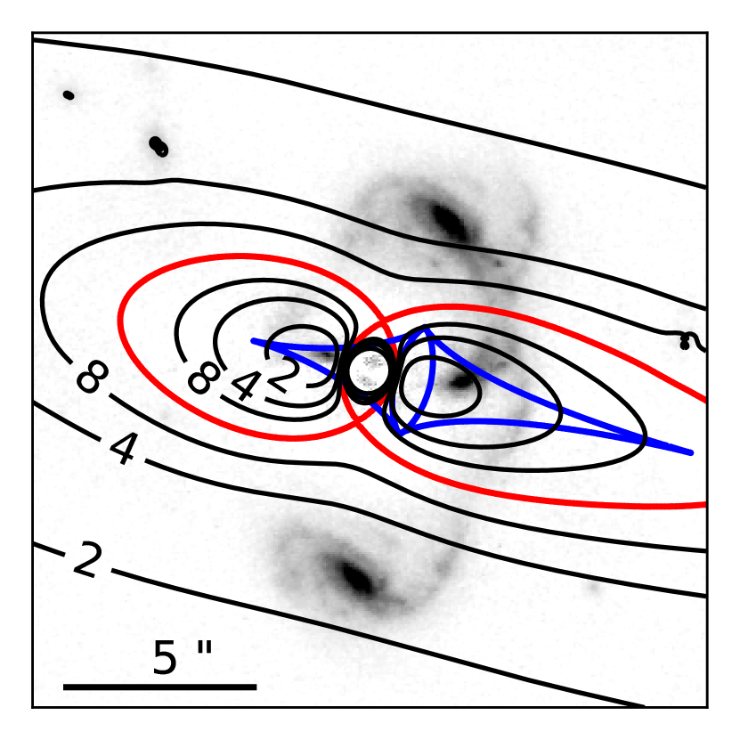
Figure 4.— Contours of the absolute value of magnification as calculated from the best-fit lens model, for a source at $z$=0.816. In red we plot the critical curve, i.e. regions in the image plane with formally infinite magnification. In blue we plot the caustic, which is the projection of the critical curve onto the source plane. In this figure north is up and east is to the left.

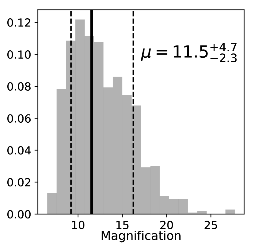
Figure 5.— The total magnification of SGAS J1438 is computed as the ratio of the total image plane area to the source plane area of the multiple images (see text). The solid line denotes the value from the best-fit model and the dashed lines mark the $1\sigma$ confidence intervals, computed from the MCMC chain.

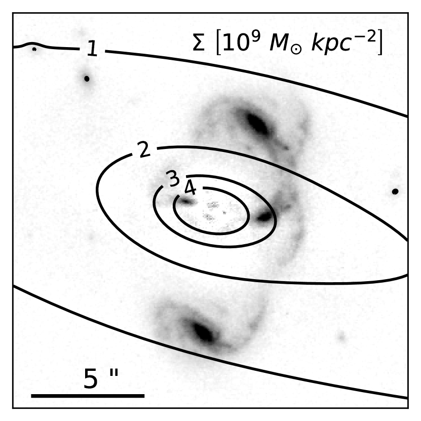
Figure 6.— The surface mass density contours from the best-fit model overplotted on the F140W image with the BCG removed. The mass density distribution is dominated by the BCG and elongated in the direction of the next brightest galaxy. In this figure north is up and east is to the left.

5. Source Plane Reconstruction

Following the procedure in Sharon et al. (2012, 2014) we ray-trace the image plane pixels from each image of the source through the lensing equation, $\vec{\beta}=\vec{\theta}-d_{ls}/d_{s}\,\vec{\alpha}(\vec{\theta})$, where $\vec{\beta}$ and $\vec{\theta}$ are the source and image positions, respectively, $d_{ls}/d_{s}$ is the ratio of the angular diameter distances from the lens to the source and from the observer to the source, and $\vec{\alpha}(\vec{\theta})$ is the deflection matrix of the best-fit model. The coordinates and shape of each pixel are translated to the source plane while conserving surface brightness. Figure 7 shows the reconstruction of the source plane from each one of the four images of SGAS J1438. Since images 2 and 4 are partial images they do not form a complete image of the source galaxy in the source plane as do images 1 and 3. In the source plane, the positions of the ray traced emission knots have a mean scatter of $0\farcs 033$, indicating the agreement between the source reconstructions of the different images.

Unlensed, the spatial extent of the galaxy in the source plane is $\sim 5$ square arcseconds, which translates to $\sim 287$ kpc² at the source redshift, $z$=0.816. The spatial extent of the source is defined by taking the area of the images, ray-tracing them back to the source-plane, and re-calculating the area in the source-plane. The source plane morphology is similar to the lensed morphology of the galaxy, indicating that the lensing potential does not introduce significant distortion. The lensing magnification is generally a combination of an isotropic magnification component due to the local projected mass density, and an anisotropic component due to shear. Low distortion indicates that in this location the lens produces little shear, resulting in nearly isotropic magnification.

6. Morphology and Distribution of Star Formation

The source plane reconstructions (Figure 7) reveal SGAS J1438 to be a large, two-arm, grand design spiral galaxy. This was suggested by the image plane morphology but is even more evident given the source plane reconstructions. The red color of the core of this galaxy and the shape of the SED published in Gladders et al. 2013 suggests that the nuclear emission is extremely obscured by dust.

In contrast, the spiral arms contain many distinct patches of emission with colors much bluer than the core, suggesting that there is widespread recent star formation in the arms that is largely unobscured by dust. At z=0.816, H$\alpha$ emission, a tracer of ongoing star formation, falls at a wavelength that does not lie within any of the three broadband filters used to observe SGAS J1438. It is, however, within the wavelength range observable in our HST WFC3/IR grism spectroscopy.

H$\alpha$ emission is not detected in the nucleus of SGAS J1438 in our grism observations. Furthermore, because of the orientation of the galaxy the brightest emission in the spiral arms of images 1 and 3 is closely aligned with the much stronger continuum emission from the nucleus in the direction of dispersion, causing the nuclear emission to drown out the signal in the spiral arms. Unfortunately, grism observations at other angles would have caused the BCG contamination to overwhelm the spectra of images 1 and 3. That same contamination, at the angles used in our grism program, makes it impossible to access the spectra of images 2 and 4. However, in image 3, the northwestern spiral arm is successfully separated from the nucleus, albeit with moderate to high contamination from the BCG. A hint of H$\alpha$ emission is visible, as shown in Figure 8. Comparing an isophote of the direct image (left panel of Figure 8) with the shape of the faint emission in the 2D grism spectrum at the wavelength of H$\alpha$ at z=0.816 (center panel) shows very faint H$\alpha$ emission coincident with the large blue clumps in the spiral arm seen on the right of panel 3 in Figure 7. A suggestion of H$\alpha$ emission from the southeastern portion of image 3 is also visible above the spectrum of the nucleus, but it is even less clear.

Because of the contamination from the BCG it is difficult to estimate the strength of the H$\alpha$ emission in the spiral arms. The fact that the H$\alpha$ emission aligns spatially with one of the blue regions in the broadband imaging bolsters the interpretation that it and the many other similarly colored regions throughout the spiral arms are regions of ongoing star-formation. Unfortunately, with these data it is difficult to comment on the star formation in the nucleus because it is so severely obscured by dust. Interestingly, Gladders et al. 2013 reported a detection of H$\alpha$ in the nucleus, which we fail to detect here. With HST-quality imaging, however, we see that there are blue clumps—likely H$\alpha$ emitters—to the south and southeast of the nucleus and hints of others to the north and northwest that were included in the slit of the Gladders et al. 2013 spectroscopy. We now believe that the nuclear H$\alpha$ emission reported in that paper is actually emission from these blue clumps that were not identifiable in extant ground-based imaging at the time.

The finding that star forming regions are large (the largest such regions are on the kiloparsec scale according to the reconstructed source image) and distributed throughout the galaxy with a morphology consistent with a grand-design spiral lends support to the interpretation that star formation occurs on galaxy-wide scales in z$\sim$1 LIRGs rather than in small (hundreds of parsecs or smaller), localized regions like in z$\sim$0 LIRGs. One caveat to this apparent galaxy-scale star formation is the deficit of observed H$\alpha$ emission in the core, which probably is not a deficit of star formation but likely reflects enhanced obscuration at that location. Unfortunately, the extant long-wavelength imaging on SGAS J1438 lack the spatial resolution to clearly demonstrate extensive obscured star formation in the core. Understanding whether or not the core is actively forming stars would be useful for understanding what physical conditions lead to this galaxy-wide mode of star formation; but in either case we have directly shown that the star formation in this z$\sim$1 LIRG is indeed occurring at much larger spatial scales than in z$\sim$0 LIRGs, as was previously expected but not directly observed.

7. Discussion

We find that the mass of the lens is consistent with a small group of galaxies (e.g., Han et al. 2015), in line with the cluster richness reported in Gladders et. al. (2013) of $N^{weighted}_{gals}=9.734$. The lens model favors a displacement of the center of the cluster halo from the BCG, at $4\farcs 88$ in the direction of the second and third brightest galaxies in this structure. A small offset between the BCG and the center of mass of the group or cluster is expected (e.g., George et al. 2012), and consistent with the light distribution of the cluster (Figure 1). Our model is in good agreement with the observed velocity dispersion of the BCG reported in Gladders et al. (2013), $\sigma_{v}=318\pm 111$ km s^-1.

The magnification of SGAS J1438 allows us to study star formation in the source galaxy in detail that would be unattainable without lensing. The typical lensing magnification of individual emission knots, a factor of 3-5, enables studies of individual star forming regions in a galaxy at $z$=0.816 with a high signal-to-noise ratio. The angular size of the source galaxy, unmagnified, is $2\farcs 53$ ($\approx 19$ kpc). In good conditions, ground-based resolution of $0\farcs 6$ would allow at best up to four non-overlapping resolution elements, dominated by the bulge. With the lensing magnification boost even ground-based observations can resolve more than ten regions in this galaxy and thus resolve its two-arm structure.

HST imaging has revealed the structure of this galaxy to be a large, two-arm, grand design spiral with a very red core and bluer clumps with sizes up to the kiloparsec scale scattered through its spiral arms. HST/WFC3 grism spectroscopy of all the images of the galaxy were severely contaminated and dominated by light of the foreground BCG; high-resolution integral field spectroscopy would overcome this issue. Nevertheless, the grism data confirm that H$\alpha$ emission is present in these clumps, though no such emission is detected in the core. The widespread star formation in the spiral arms supports previous interpretations of the spatially unresolved spectra of z$\sim$1 LIRGs, namely that such objects are likely to have large scale, nearly galaxy-wide star formation, in contrast to their counterparts in the local universe where star formation can be intense but occurs on smaller scales.

Based on observations made with the NASA/ESA Hubble Space Telescope, obtained at the Space Telescope Science Institute, which is operated by the Association of Universities for Research in Astronomy, Inc., under NASA contract NAS 5-26555. These observations are associated with program #14420.

Parameter	Cluster	BCG
R.A. [′′]	$4.34^{+1.06}_{-2.86}$	[$0$]
Decl. [′′]	$-1.08^{+0.73}_{-0.34}$	[$0$]
e	$0.87^{+0.07}_{-0.13}$	$0.47^{+0.08}_{-0.36}$
$\theta$ [°]	$165^{+2}_{-1}$	$168^{+28}_{-29}$
$r_{core}$ [kpc]	$31^{+39}_{-31}$	$1.58^{+2.87}_{-0.67}$
$\sigma$ [km/s]	$606^{+3}_{-96}$	$281^{+39}_{-51}$
$r_{cut}$ [kpc]	[$1000$]	[$20$]

Note. — Best-fit values from the image plane optimization. The coordinates of the BCG are fixed at their observed location, (R.A., Decl.) = (219.68768, 14.903482). The position of the cluster halo is measured relative to the BCG. The position angle $\theta$ is measured north of west, and the ellipticity of the projected mass density is $e=(a^{2}-b^{2})/(a^{2}+b^{2})$, where $a$ and $b$ are the semi-major and semi-minor axes, respectively. The core radius of the cluster was not well-constrained by the model, and so the uncertainties quoted here are the priors set for the MCMC optimization.

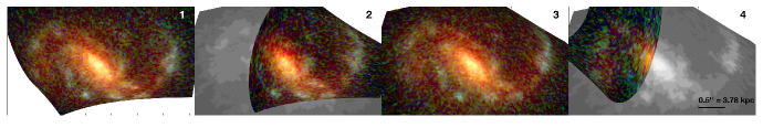
Figure 7.— SGAS J1438 is reconstructed from each of its four images by ray-tracing the image-plane pixels through the deflection of the best-fit lens model. Images 1 and 3 form complete images of the source, while images 2 and 4 are partial images, due to their location with respect to the source plane caustic. The grayscale background in panels 2 and 4 is to guide the eye to the extent of the full image of the source, and is replicated from image 3. For context, the source plane scale is given as a horizontal bar.

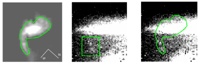
Figure 8.— Left: Direct image of SGAS J1438 image 3 in the F140W filter, with an isophote drawn as a reference for the object’s shape. Center: The 2D spectral extraction from HST WFC3/IR G141 grism spectroscopy data, showing a very faint H$\alpha$ detection (marked by the box) below the bright nuclear continuum emission. Right: The isophote from the leftmost panel on top of the 2D grism spectral extraction in the center panel, with the isophote placed so that the flux weighted center of the direct image would lie at the wavelength of H$\alpha$ emission at the redshift of SGAS J1438. Note that the slight flux excess noted in the center panel lies inside the the spiral arm, aligned closely with the emission in the direct image.

References

- Bayliss et al. (2014) Bayliss, M. B., Rigby, J. R., Sharon, K., et al. 2014, ApJ, 790, 144
- Bordoloi et al. (2016) Bordoloi, R., Rigby, J. R., Tumlinson, J., et al. 2016, MNRAS, 458, 1891
- Elbaz et al. (2010) Elbaz, D., Hwang, H. S., Magnelli, B., et al. 2010, A&A, 518, L29
- Farrah et al. (2008) Farrah, D., Lonsdale, C. J., Weedman, D. W., et al. 2008, ApJ, 677, 957
- George et al. (2012) George, M. R., Leauthaud, A., Bundy, K., et al. 2012, ApJ, 757, 2
- Gladders et al. (2000) Gladders, M. D., & Yee, H. K. C. 2000, AJ, 120, 2148.
- Gladders et al. (2013) Gladders, M. D., Rigby, J. R., Sharon, K., et al. 2013, ApJ, 764, 177
- Gonzaga & et al. (2012) Gonzaga, S., & et al. 2012, Hubble Space Telescope Primer for Cycle 21
- Gonzaga & et al. (2012) Gonzaga, S., & et al. 2012, The DrizzlePac Handbook, HST Data Handbook
- Hwang et al. (2010) Hwang, H. S., Elbaz, D., Magdis, G., et al. 2010, MNRAS, 409, 75
- Han et al. (2015) Han, J., Eke, V. R., Frenk, C. S., et al. 2015, MNRAS, 446, 1356
- Johnson & Sharon (2016) Johnson, T. L., & Sharon, K. 2016, ApJ, 832, 82
- Johnson et al. (2017) Johnson, T. L., Rigby, J. R., Sharon, K., et al. 2017, ApJ, 843, L21
- Jullo et al. (2007) Jullo, E., Kneib, J.-P., Limousin, M., Elíasdóttir, Á., Marshall, P. J., & Verdugo, T. 2007, New Journal of Physics, 9, 447
- Limousin et al. (2005) Limousin, M., Kneib, J.-P., & Natarajan, P. 2005, MNRAS, 356, 309 2001, ApJ, 563, 9
- Meneghetti et al. (2010) Meneghetti, M., Rasia, E., Merten, J., et al. 2010, A&A, 514, A93
- Menéndez-Delmestre et al. (2009) Menéndez-Delmestre, K., Blain, A. W., Smail, I., et al. 2009, ApJ, 699, 667
- Ofek (2014) Ofek, E. O. 2014, Astrophysics Source Code Library, ascl:1407.005
- Papovich et al. (2007) Papovich, C., Rudnick, G., Le Floc’h, E., et al. 2007, ApJ, 668, 45
- Peng et al. (2002) Peng, C. Y., Ho, L. C., Impey, C. D., & Rix, H.-W. 2002, AJ, 124, 266
- Peng et al. (2010) Peng, C. Y., Ho, L. C., Impey, C. D., & Rix, H.-W. 2010, AJ, 139, 2097
- Rigby et al. (2008) Rigby, J. R., Marcillac, D., Egami, E. et al. 2008, ApJ, 675, 262
- Rowan-Robinson et al. (2004) Rowan-Robinson, M., Lari, C., Perez-Fournon, I., et al. 2004, MNRAS, 351, 1290
- Rowan-Robinson et al. (2005) Rowan-Robinson, M., Babbedge, T., Surace, J., et al. 2005, AJ, 129, 1183
- Rujopakarn et al. (2011) Rujopakarn, W., Rieke, G. H., Eisenstein, D. J., & Juneau, S. 2011, ApJ, 726, 93
- Sajina et al. (2006) Sajina, A., Scott, D., Dennefeld, M., et al. 2006, MNRAS, 369, 939
- Sharon et al. (2012) Sharon, K., Gladders, M. D., Rigby, J. R., et al. 2012, ApJ, 746, 161
- Sharon et al. (2014) Sharon, K., Gladders, M. D., Rigby, J. R., et al. 2014, ApJ, 795, 50
- Symeonidis et al. (2009) Symeonidis, M., Page, M. J., Seymour, N., et al. 2009, MNRAS, 397, 1728
- Wuyts et al. (2012) Wuyts, E., Rigby, J. R., Sharon, K., & Gladders, M. D. 2012, ApJ, 755, 73.