ALTSched: Improved Scheduling for Time-Domain Science with LSST
Abstract
Telescope scheduling is the task of determining the best sequence of observations (pointings and filter choices) for a survey system. Because it is computationally intractable to optimize over all possible multi-year sequences of observations, schedulers use heuristics to pick the best observation at a given time. A greedy scheduler selects the next observation by choosing whichever one maximizes a scalar merit function, which serves as a proxy for the scientific goals of the telescope. This sort of bottom-up approach for scheduling is not guaranteed to produce a schedule for which the sum of merit over all observations is maximized. As an alternative to greedy schedulers, we introduce ALTSched, which takes a top-down approach to scheduling. Instead of considering only the next observation, ALTSched makes global decisions about which area of sky and which filter to observe in, and then refines these decisions into a sequence of observations taken along the meridian to maximize SNR. We implement ALTSched for the Large Synoptic Survey Telescope (LSST), and show that it equals or outperforms the baseline greedy scheduler in essentially all quantitative performance metrics. Due to its simplicity, our implementation is considerably faster than OpSim, the simulated greedy scheduler currently used by the LSST Project: a full ten year survey can be simulated in 4 minutes, as opposed to tens of hours for OpSim. LSST’s hardware is fixed, so improving the scheduling algorithm is one of the only remaining ways to optimize LSST’s performance. We see ALTSched as a prototype scheduler that gives a lower bound on the performance achievable by LSST.
1 Introduction
LSST is a large ground-based survey system scheduled to begin operations in 2022. With the capability to survey the entire southern sky in 6 bands about once a week, LSST will enable time-domain astronomy at an unprecedented scale. The telescope was designed with four primary science goals in mind: to understand dark matter and dark energy; to catalog the solar system; to study the structure and formation of the Milky Way; and, perhaps most uniquely suited to LSST’s particular characteristics, to explore the large frontier of time-domain astronomy. These science goals motivate a range of competing technical metrics that LSST should optimize. Presenting a full list of science cases for LSST and accompanying technical metrics is beyond the scope of this paper; we refer readers to the LSST observing strategy whitepaper (LSST Science Collaborations et al., 2017). Here we present only a few representative examples (with science cases in parentheses), which we believe are especially sensitive to scheduling decisions:
| long observing seasons (parallax measurements, AGN variability, few-months-long transients) | high cadence (faster transients, better characterization of light curves) | |
| large survey area (large-scale structure, weak lensing, galaxy/star surveys) | higher co-added depth (studying fainter objects) | |
| few filter changes (maximize survey efficiency) | many filter changes (obtain nightly colors for variables & transients) | |
| large overlap between neighboring observations (rapid revisits for very fast transients) | small overlap between neighboring observations (cover a larger area per unit time) | |
| multiple observations per field per night (link asteroids, probe ~hour-scale variability) | one observation per field per night (transients that don’t change in ~1 hour) | |
With the LSST Project well into the construction phase, the system’s hardware characteristics (aperture, field size, slew rate, field of view, sensor quantum efficiency…) are fixed. Apart from actively engineering the weather in Chile, the only remaining opportunities to extract additional performance from the LSST system are in the scheduler and in the data reduction pipeline. LSST’s existing scheduler, called OpSim, is a greedy algorithm: it chooses the next field to observe by maximizing a scalar merit function intended as a proxy for the scientific merit of observing the field. This approach is appealing in its apparent simplicity, but as we show below, even after over a decade of development, OpSim under-performs on many science metrics, particularly in the time-domain science so critical to LSST’s mission. We argue here that the fault lies not in any implementation detail, but rather in the fundamental nature of greedy algorithms: because they make scheduling decisions only one or a few observations in advance, the parameters of the algorithm give scientists little or no control over many 10-year global properties of the schedule.
To remedy this, we introduce and analyze an alternative scheduling algorithm, ALTSched, which makes scheduling decisions with a top-down hierarchical approach, instead of using a purely bottom-up local merit function. We defer a full description of ALTSched to Section 3, but simply put, our algorithm first decides which region of sky to observe (nightly), then which particular area and filter to use (hourly), and only then which individual pointings to observe (minute-scale). In contrast, OpSim chooses every next observation ab initio, with no planning horizon larger than 30 seconds and no global strategy except what is encoded indirectly through the merit function.
One major advantage of ALTSched is that the parameters of the algorithm directly control final properties of the schedule. For example, ALTSched observes either the Northern or Southern sky each night. Because LSST can observe about half of the sky each night, we can obtain a universal 2-day revisit cadence simply by assigning even-numbered nights to the Northern sky and odd-numbered nights to the Southern sky. Different cadences (e.g. with some 1- and 3-day revisits) are equally simple with a different pattern of North and South. Importantly, there is no known way to similarly modify this distribution of revisit times in OpSim, except by adjusting the weights and penalties of the merit function specifically to mimic the exact behavior of ALTSched.
As of the writing of this paper, the LSST Project is planning to run a suite of OpSim simulations in order to choose a final observing strategy for LSST. One point of this paper is to argue that optimizing over the parameters of OpSim in this way will not yield an optimal survey strategy. Taking the example above one step further before giving a fuller analysis in 4, the gaps between observations to a particular sky pixel resemble an exponential distribution for every OpSim run we have analyzed, over a wide range of OpSim’s parameters. An exponential distribution of revisit times is consistent with the timing of observations following a random process. In ALTSched, the shape of this distribution can be easily controlled. Instead of running more and more OpSim simulations, we therefore advocate exploring how OpSim can be made to reproduce the survey strategy of ALTSched, and how ALTSched’s cadence can be further improved.
In the sections that follow, we first summarize the LSST baseline scheduler and the tools used to assess the scientific performance of various alternatives. We then describe the implementation of our alternative scheduler, ALTSched, and make quantitative performance comparisons to the LSST baseline. We close with a discussion and some suggestions for future work.
2 OpSim
To provide context for ALTSched, the algorithm we propose below, we first introduce LSST’s current baseline scheduling algorithm.111The LSST scheduler is undergoing continual development, and the version of OpSim described and compared with in this article has been superseded, but it was the baseline plan at the time this work was completed.
LSST’s current scheduler is part of a package called the Operations Simulator (OpSim) (Delgado & Reuter, 2016). OpSim uses a greedy algorithm to choose fields based on a proposal system, where abstractions of different scientific proposals give a score for each candidate field, and the scheduler chooses the field with the highest combined score, or merit. OpSim considers a number of criteria in its merit function, including time since last observation, co-added depth achieved thus far, airmass and sky brightness at the proposed pointing, slew time to reach the pointing, etc. For a full description of the complex merit function used for minion_1016, we refer readers to Delgado et al. (2014, §5). Once an observation is chosen and executed, the merit scores are recalculated for every candidate field, and the process repeats. The parameters of OpSim are the weights and penalties associated with the various inputs to the merit function. Although easily interpretable in the context of local decision making, these parameters have no simple connection to many of the scheduling decisions we actually want to make: the average and distribution of season lengths and of revisit times; the colors (or lack thereof) obtained during a single night; the uniformity of light curve sampling over time; etc. In contrast, as we show below, ALTSched’s parameters directly control these properties.
Included with OpSim is a module that simulates the system hardware, weather, seeing conditions, and downtime. For fairness of comparison, ALTSched uses the exact same calculations, though we re-implement the simulator to improve computational efficiency. In particular, we obey all physical constraints on the telescope, including making no observations below LSST’s minimum elevation or in the zenith avoidance area, accounting for readout time, shutter time, slew speed, settle time, optics correction time, and filter change time, only using 5 of LSST’s 6 band-pass filters per night, etc. Taking slew time as an example: both OpSim and ALTSched use the same slew calculation, described in Delgado et al. (2014, §6). In short, the slew time is calculated assuming uniform accelerated motion of the telescope mount and dome, plus some settle time.
To compare simulated surveys, the LSST Project has developed a useful suite of analysis tools, the Metrics Analysis Framework (MAF), that can evaluate candidate schedules by computing various performance metrics of interest (Jones et al., 2014). Examples include the number of type Ia supernova light curves that meet certain criteria, the distribution of co-added depths over the observed region, the anticipated uncertainty in parallax and proper motion measurements. This framework is critical for the fair evaluation of simulated surveys.
A number of OpSim runs, or simulated surveys, have been released by the Project. At the time this work was carried out, the baseline simulated survey was minion_1016, and we compare our results to those of minion_1016. Later versions of OpSim have improved on a number of metrics, but all runs we have analyzed since minion_1016 suffer from poor time-domain performance. For example, none of the cadences released with the recent whitepaper call recover even half as many well-sampled SNIa without eliminating visit pairs or changing the exposure time (where “well-sampled” is as defined below). And to our knowledge, no OpSim or feature-scheduler run at all has exceeded ALTSched in this metric. Results for minion_1016 are presented in more depth in Section 4.
Several alternatives to OpSim have also been proposed. Naghib et al. (2016) frame the scheduling problem as a Markovian decision process. Ridgway (2015) proposes scheduling LSST by dividing observing into blocks that are observed (and then reobserved) in an optimal manner. Ridgway’s proposal is similar in spirit to the algorithm developed and described in this paper.
3 ALTSched
In this section, we introduce ALTSched, an alternative scheduling algorithm for LSST. In the next section, we introduce a number of metrics, and demonstrate quantitatively that ALTSched equals or outperforms the existing OpSim baseline minion_1016 on these metrics.
3.1 ALTSched Algorithm
ALTSched is a deterministic scheduling algorithm: in a given night, it does not adapt to current weather or seeing conditions. Although in principle, adjusting a schedule to take prevailing weather conditions into account should only improve a scheduler, we justify our decision to use a non-adaptive algorithm in three ways: 1) maintaining a consistent cadence – i.e. avoiding long observation gaps – is difficult to do if the scheduler aggressively avoids regions with poorer observing conditions, since by random chance, some regions will go unobserved for a long time; 2) the best seeing tends to occur on the meridian (at minimum airmass), which is where ALTSched observes anyway; 3) one strength of ALTSched is that it achieves such high performance even without dynamically reacting to observing conditions. We only expect our performance to improve with the judicious addition of poor-weather avoidance.
The algorithm itself is remarkably simple. Each night, it chooses whether to observe the Northern or Southern sky based on which region has received fewer visits so far, and then during the night it scans North and South of the meridian, taking 30-second exposures and then slewing by approximately one field width. LSST is on an alt/az mount, and so has a zenith-avoidance area. To observe the region of sky that passes over zenith, we therefore periodically scan to the East and West over that region. Each N/S scan is repeated twice in order to obtain two observations per night, separated by roughly 30-60 minutes. Before repeating a scan, we change filters so that every field is visited in two bands per night. We refer readers to the video in the supplementary material; the scanning strategy is much more easily explained visually than in text.
The exact pointings used are drawn from a fixed tiling that is randomly rotated by much more than a field size each night. If a pointing is not used in a given night, it is saved for use in a later night, so that gaps do not persist. The fixed tiling is chosen as a solution to the Thomson charge-distribution problem for (Thomson, 1904).
3.2 Moon Avoidance
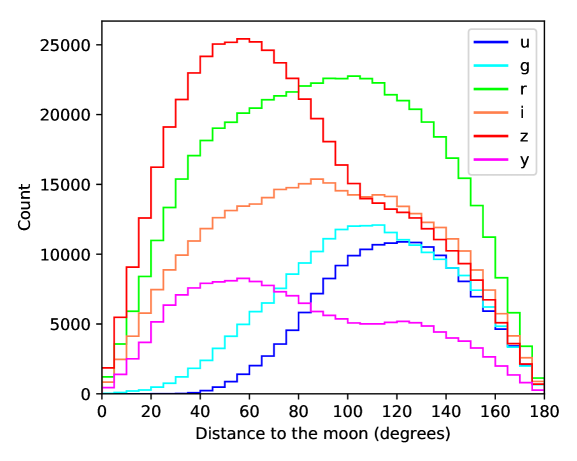
One deficiency in ALTSched is that it contains no provision for avoiding the moon. minion_1016 uses a conservative avoidance radius of . This corresponds to 7% of the celestial sphere, so about 7% of observations should fall within this avoidance zone. However, is likely too conservative in times near a new moon and in the redder filters. We therefore expect only a few percent of observations to be problematically close to the moon. For observations that fall too close to the moon, the simulated sky brightness is very high, leading to a low limiting depth for those observations. So any metric depending on depth should only improve by adding a moon-avoidance module to ALTSched. Figure 1 shows histograms of the angular distance between ALTSched’s observations and the moon. Note that ALTSched avoids observing in the u and g bands at all when the moon is up and bright, so there are few or no observations in u or g closer than to the moon.
3.3 Filter Allocation
Most simulated surveys of LSST assume that the telescope will visit each field twice per night, with a separation of minutes, in order to link asteroid observations. To improve the cadence in each band, ALTSched usually carries out these two visits in different filters. To accomplish this with a minimal number of filter changes, we divide observations into blocks that take minutes to observe, and we visit each block twice back-to-back, changing filters before revisiting a block (but not between the revisit of a block and the first visit to the subsequent block). The video in the supplementary materials demonstrates this filter allocation strategy. On average, we execute filter changes per night, compared to minion_1016’s . This adds seconds to our average slew time over minion_1016, and allows us to double cadence in each band.
Our filter allocation strategy is designed such that, in theory, visits to every sky pixel will cycle through the six filters in order. Assigning numbers 1 through 6 to LSST’s 6 bandpass filters (), and using arithmetic modulo 6, we start a night in some filter , and during the night, before every revisit block, we switch from filter to filter . The next night starts in filter and the process repeats, ensuring that visits to each pixel cycle through all six filters. In the ideal case, every sky pixel gets a visit in every band once every 6 nights (2 bands every 2 nights, since we alternate observations between the northern and southern sky).
However, many factors cause us to deviate from this ideal strategy. First, we don’t want a uniform distribution of total number of visits over filters, so we replace some observations in, say, the band, with more in instead. Second, we observe and preferentially in twilight, since these bands are less sensitive to high sky brightness. Third, we avoid using or when the moon is up and bright. And lastly, the filter changer can only fit 5 of LSST’s 6 filters, so only 5 filters can be used in a single night. In each of these cases, if a filter is “not allowed” during a time when the cyclic allocation strategy would have scheduled it, we simply use some other filter instead. Besides these intentional deviations, weather and downtime also cause us to deviate from this ideal strategy in ways that are less predictable.
Overall, ALTSched’s filter allocation strategy ensures that the per-band cadence is much more regular than in minion_1016 (as shown below), but there is likely much room for improvement by designing a strategy that more intelligently takes the four deviations from ideal described above into account.
4 Metrics & Results
As laid out in Section 1, the science drivers of LSST motivate a wide range of technical metrics, many of which are in tension with each other. Broadly speaking, LSST’s science goals fall into two categories: those that depend mainly on the final co-added images (static science), and those that depend mainly on the temporal distribution of visits throughout the survey (time-domain science). A full list of results on a variety of metrics is available at http://altsched.rothchild.me:8080. Here we highlight a small subset of these metrics that are particularly sensitive to scheduling decisions, especially those where ALTSched and minion_1016 achieve different results.
4.1 Static Science
A number of science drivers (e.g. galaxy/star surveys, large-scale structure measurements) use co-added images, and are largely insensitive to the exact distribution of visits over time. A wide range of static science is enabled by achieving a higher final co-added depth in each band. We therefore use co-added depth as a chief metric for static science. Single-visit depths and full 10-year co-added depths are shown for both schedulers in Table 1. Since different survey strategies may allocate visits across filters differently, we summarize the total co-added performance across bands with the effective survey time metric . Given design limiting depths for a 30-second exposure in filter , the effective survey time of a series of exposures which achieved a limiting depth in filter is given by
The limiting depth of an exposure is computed taking into consideration the sky brightness, seeing, and airmass, as described in equation 6 of Ivezic et al. (2008). Design depths for LSST are shown in Table 1. These design depths assume an airmass of , -band seeing of arcsec (FWHM), and -band sky brightness of 21 mag/arcsec2. In practice, observations are taken under worse conditions, so the total is surprisingly low for a 10-year survey.
| u | g | r | i | z | y | |
|---|---|---|---|---|---|---|
| Design (Ideal) Single-Visit Depths | 23.9 | 25.0 | 24.7 | 24.0 | 23.3 | 22.1 |
| Median Single-Visit Depth (minion_1016) | 23.09 | 24.51 | 24.05 | 23.45 | 22.71 | 21.78 |
| Median Single-Visit Depth (ALTSched) | 23.21 | 24.50 | 23.93 | 23.49 | 22.90 | 21.91 |
| Median Co-added Depth (minion_1016) | 25.48 | 27.02 | 27.03 | 26.46 | 25.65 | 24.73 |
| Median Co-added Depth (ALTSched) | 25.61 | 27.03 | 27.04 | 26.35 | 25.93 | 24.31 |
Two related metrics are the average slew time (including filter changes), and the open-shutter fraction, defined as:
where is the exposure time, and consists of any intermediate readout time between back-to-back “snaps” during the same visit (the readout after the last snap is included in the slew time). Both minion_1016 and ALTSched divide 30-second visits into 2 15-second snaps for cosmic-ray rejection.
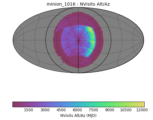
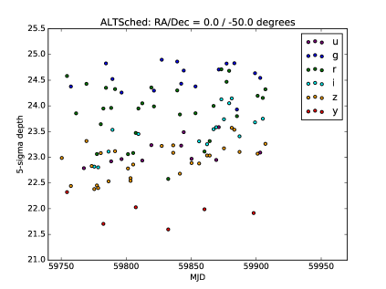
Maximizing is one motivation for ALTSched’s meridian-scanning strategy, since observing fields at their minimum airmass yields the highest depth. Results for these three metrics are shown in Table 2. Despite achieving a lower and higher average slew time, ALTSched reaches approximately the same as minion_1016, since minion_1016 observes off the meridian, as shown in Figure 2. In particular, in LSST’s wide-fast-deep region, minion_1016 achieves a mean (median) airmass of 1.22 (1.21) compared to ALTSched’s 1.12 (1.09). minion_1016’s mean (median) normalized airmass – i.e. the airmass of an observation divided by the minimum airmass that field could have been observed at – is 1.16 (1.14) compared to 1.05 (1.01) for ALTSched. ALTSched suffers from a higher slew time for three reasons: first, because we change filters much more often than minion_1016 in order to obtain same-night colors for nearly every visit; second, because our scanning strategy is simple and could be optimized for faster slews; and third, because our sky tiling is spaced farther apart than the tiling used in OpSim.
| Avg. Slew | |||
|---|---|---|---|
| minion_1016 | 333 days | 0.72 | 7.4222The average slew time reported elsewhere for minion_1016 is 6.8 seconds. However, the current version of the LSST software stack, which we use for ALTSched, produces a value of 7.4, which is the value that is comparable to the 11.1 seconds we report for ALTSched. |
| ALTSched | 329 days | 0.69 | 11.1 |
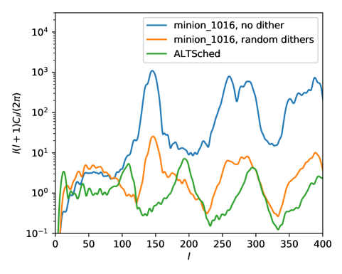
Another important consideration for static science is that of survey uniformity. In particular, weak lensing and large-scale structure measurements depend sensitively on the uniformity of co-added depth across the sky (Awan et al., 2016). OpSim uses a set of fixed field centers, and attempts to mitigate the resulting imprint on the co-added depth maps by dithering around those field centers. However, every dithering strategy tried thus far still leaves a discernible imprint on the final co-added depth maps. Instead of dithering, ALTSched eliminates fixed fields entirely. We use a fixed tiling for the entire survey, but every night, we randomly rotate this tiling by much more than a field size. Pointings not visited in a night are scheduled in a subsequent night, so gaps in the tiling pattern do not persist. To measure survey uniformity, we include angular power spectra of the number of visits to a sky pixel, shown in Figure 3. ALTSched’s tiling strategy reduces power at most angular scales, including around , where cosmological probes are particularly sensitive.
Unlike any strategy using fixed fields with dithering, our method admits simple analysis that yields an expression for the uniformity in number of visits to a sky pixel. For the fixed tiling used throughout the survey, let be the areas of sky covered by 0, 1, and 2 pointings, respectively. Assume no sky pixels are observed more than twice, so the total area covered by the tiling . Then the standard deviation of number of visits to a sky pixel using our strategy – i.e. after applying the randomly-rotated tiling times – is
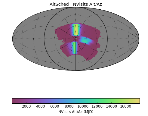
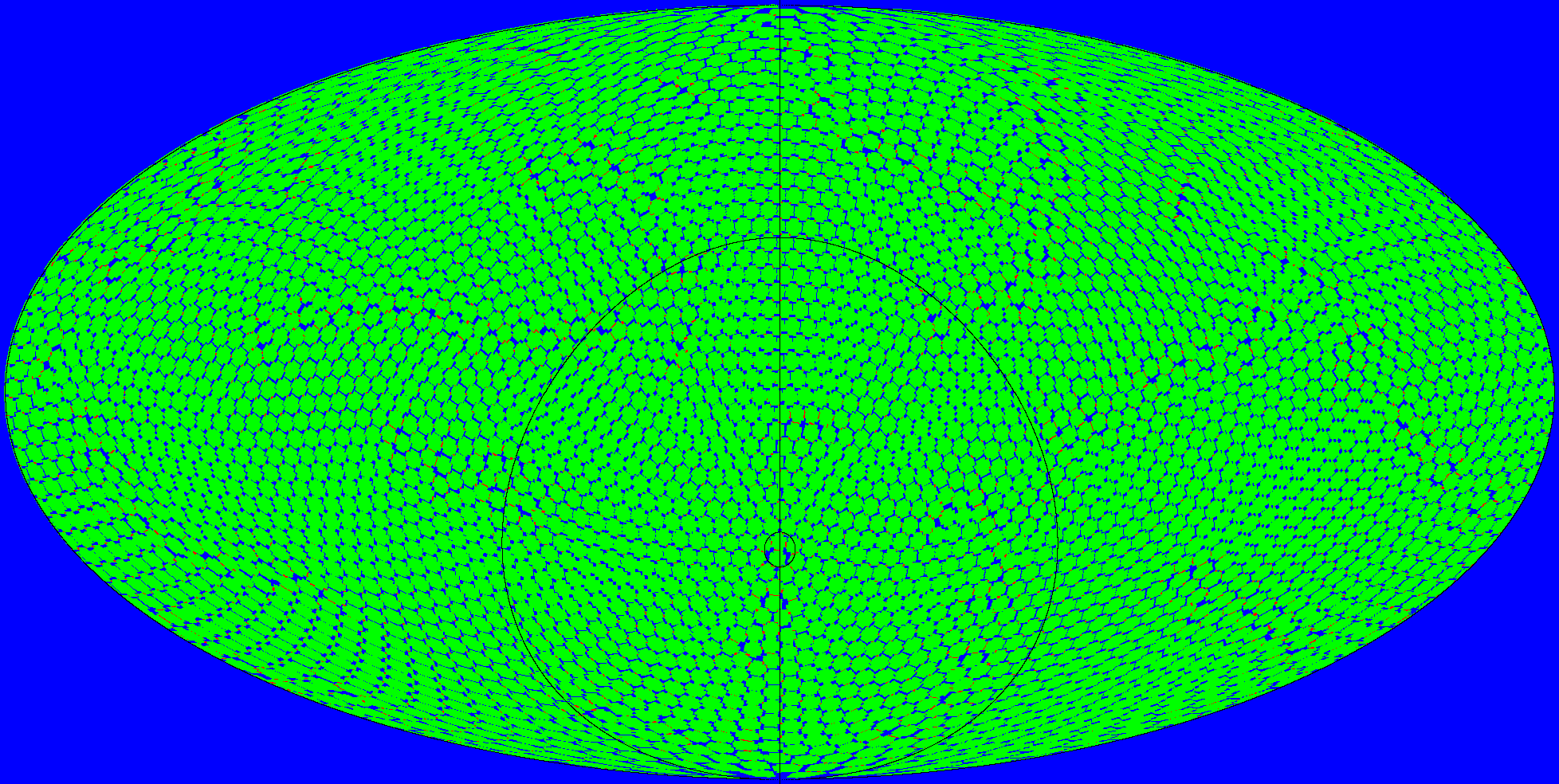
See Appendix C for a brief derivation. Note that this expression does not depend on the tiling itself – only on the . In order to minimize slew time while maintaining an even cadence, we choose a tiling with the fields evenly spaced and with . Even with , we achieve some fast revisits due to pointings held over from previous nights, which will overlap randomly with the current night’s pointings. To make the fields “evenly spaced”, we draw pointings from a solution to the Thomson charge-distribution problem for Thomson (1904). See Figure 4 for a visualization of our tiling. Adjusting changes the density of the tiling, which controls the tradeoff between the frequency of rapid revisits and the area observed per night.
4.2 Time-Domain Science
Optimizing time-domain science is much more about managing tradeoffs between different science cases than maximizing certain quantities. We argue in this section that 1) the parameters of ALTSched directly control these tradeoffs, whereas in OpSim, the tradeoffs are difficult or impossible to control, and 2) the ALTSched simulation analyzed in this paper enables a wider range of science cases than minion_1016.
Most existing simulations assume that LSST will carry out pairs of visits separated by minutes (to link asteroid observations), and will take 30-second exposures during each visit. Some OpSim simulations have been run to explore deviating from these assumptions, but here we take them as given. In this section, we explore how the distribution of visits over time affects time-domain science tradeoffs, and describe how these tradeoffs can be controlled in ALTSched and OpSim.
One fundamental tradeoff in time-domain science is between the mean season length and the mean inter-night gap (or mean cadence), which is the mean duration between consecutive visits to a sky pixel. Controlling this tradeoff with ALTSched is simple: instead of scanning along the meridian, the scheduler can start the night either East (shorter season/higher mean cadence) or West (longer season/lower mean cadence) of the meridian, and slowly move West/East over the course of the night. In contrast, there is no direct way to control this tradeoff with a greedy scheduler like OpSim. The simplest way would be to relax the airmass/hour angle penalty and hope that the scheduler makes full use of the additional area it can use. However, this is exactly what minion_1016 does, and instead of increasing the season length, it simply observes at a higher, but mostly fixed, airmass (see Figure 2). Alternatively, one could adjust the penalty on the hour angle throughout the night in order to persuade the scheduler to start observing in, say, the East, and then move over to the West by the end of the night. This might achieve the desired result, but would require tuning of weights just in order to reproduce the simple behavior already achieved by ALTSched.
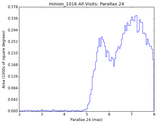
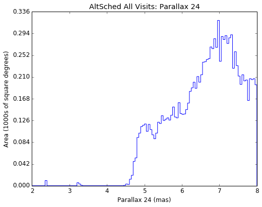
In practice, we observe along the meridian throughout the night, since we don’t see an advantage in changing the season length/mean cadence at the expense of lowering SNR by observing at higher airmass. Because minion_1016 observes at a wider hour angle range, and therefore has a slightly longer season length, one might worry that ALTSched suffers in parallax performance. However, this is not the case, as shown in Figure 5.
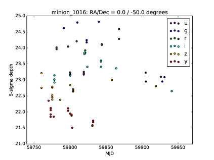
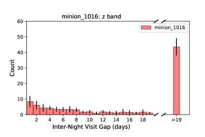
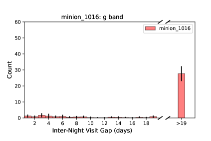
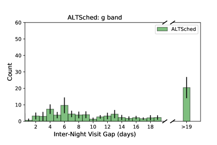
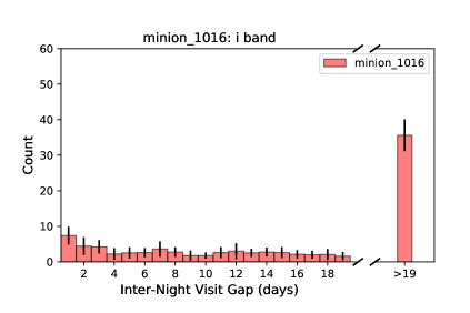
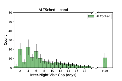
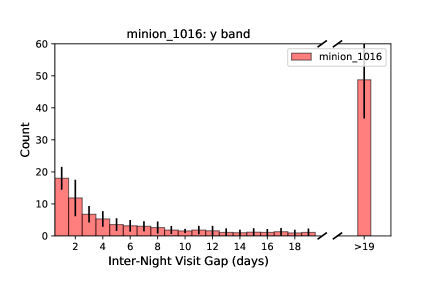
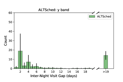
Although the mean inter-night gap is largely determined by observing efficiency and the season length, as described above, the actual distribution of inter-night gaps, measured with an inter-night gap histogram, is much more sensitive to the scheduling algorithm. This metric, though often disregarded, has a large impact on the quality of the light-curves LSST will measure. To get an intuitive sense for how the scheduling algorithm can affect the inter-night gap histogram, consider Figure 6, which shows, for a randomly chosen sky pixel, the cadences achieved by minion_1016 and ALTSched. Notice that minion_1016 often observes this pixel many times in quick succession, and then goes many days without any re-observations. In contrast, ALTSched observes this pixel with a much more regular cadence. This intuition is quantified with histograms of the gaps between consecutive visits to a sky pixel, shown in Figures 7 and 8.
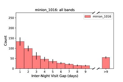
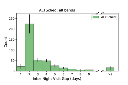
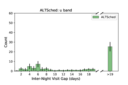
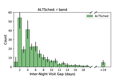
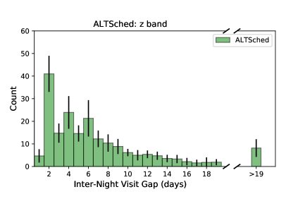
Controlling the inter-night gap histogram with ALTSched is also simple. Changing the mean season length/mean cadence as described above yields a simple scaling of the histogram in the x-axis. And the location of the peak can be tuned either by changing the number of visits to a field per night, or by employing a rolling cadence. Both options are directly controllable in ALTSched. The sharpness of the peak can also be controlled, simply by judiciously choosing which nights the telescope observes North vs. South. In the default version of ALTSched, the scheduler observes North and South on alternating nights, yielding a sharp peak in the inter-night gap histogram at 2 days. However, choosing a repeating sequence such as N N S N S S N S would yield a flatter peak at 2 days, with half the histogram mass at 2 days, and the other half distributed between 1 and 3 days. In contrast, every inter-night gap histogram we have measured from an OpSim simulation (even for simulations released after minion_1016) has looked roughly exponential. Note that an exponential distribution of inter-night gaps is consistent with an unconstrained stochastic process about the mean. We infer from this that none of the tunable parameters in OpSim explored so far have a discernible impact on the shape of the inter-night gap histogram.
Many science cases for LSST rely on approximately month-long transients (supernovae, kilonovae, tidal disruption events, etc.). For these science cases, we expect that multi-week long gaps will severely reduce the quality of light curves, without a commensurate increase in quality from the higher rate of sampling over small sections of the light curve. This intuition is borne out in simulations, run by Nicolas Regnault, Philippe Gris, and the Paris Supernovae Cosmology Team, of the number of well-sampled type Ia supernovae different simulated schedules would obtain (personal communication). As shown in Table 3, ALTSched achieves an eightfold increase in the number of well-sampled SNeIa, and also an increase of 0.07 in the maximum redshift at which the type-Ia supernova sample is complete. Although these simulations are for SNeIa in particular, we expect similar results to hold for other transients. For example, Cowperthwaite et al. (2019) find that ALTSched achieves a nearly 2x increase in the number of serendipitous kilonovae discoveries compared to minion_1016. Similarly, Goldstein et al. (2018) find that ALTSched discovers lensed supernovae earlier than minion_1016, enabling faster spectroscopic follow-up.
| Avg. | ||
|---|---|---|
| minion_1016 | 47,000 | 0.30 |
| ALTSched | 366,000 | 0.37 |
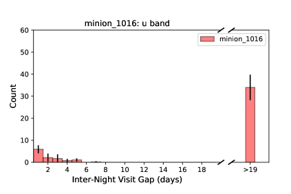
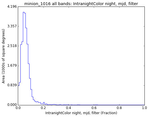
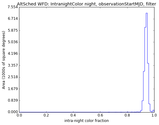
ALTSched achieves more favorable inter-night gap histograms than minion_1016 for two main reasons. The band-agnostic gaps (Figure 7) are improved because ALTSched alternates between observing the northern and southern skies each night, suppressing 1-day revisit gaps. Because the mean cadence is approximately conserved across schedulers with similar numbers of total visits, this by necessity eliminates most of the long gaps, which are so detrimental for transient characterization. The per-band gaps (Figure 8) are improved since we carry out the two visits each sky pixel receives per night in different filters, doubling the cadence in each band (see Figure 9).
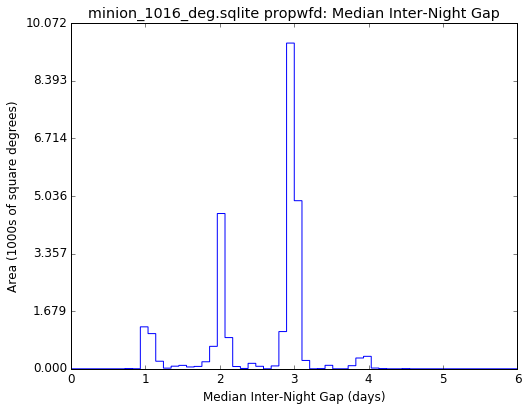
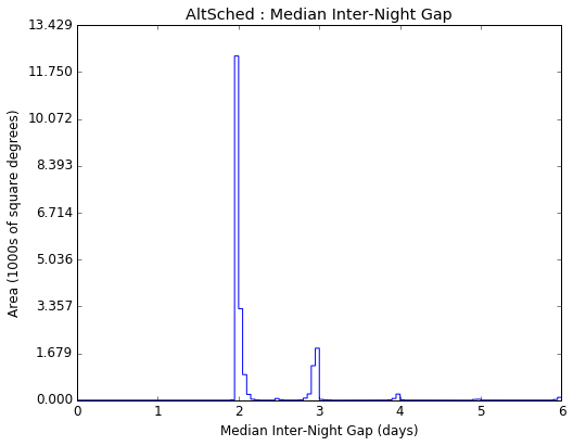
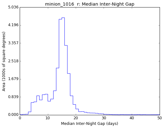
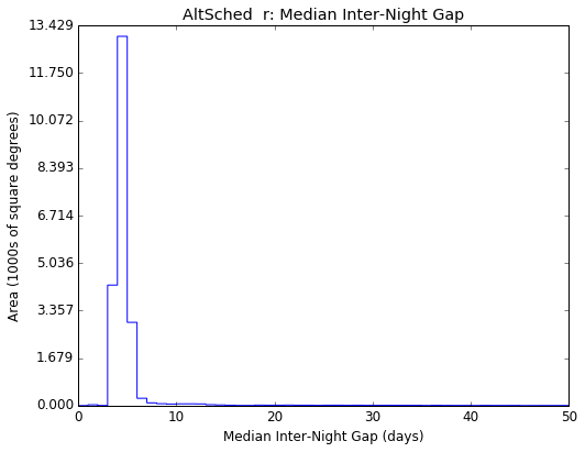
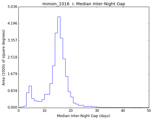
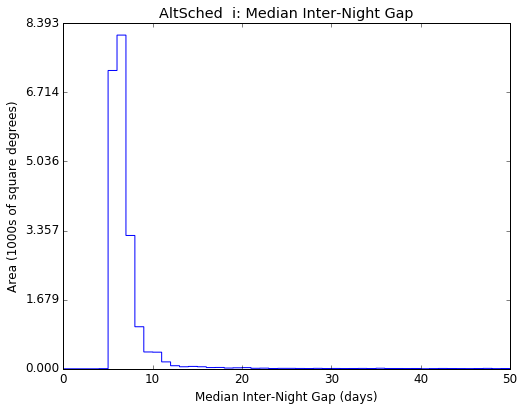
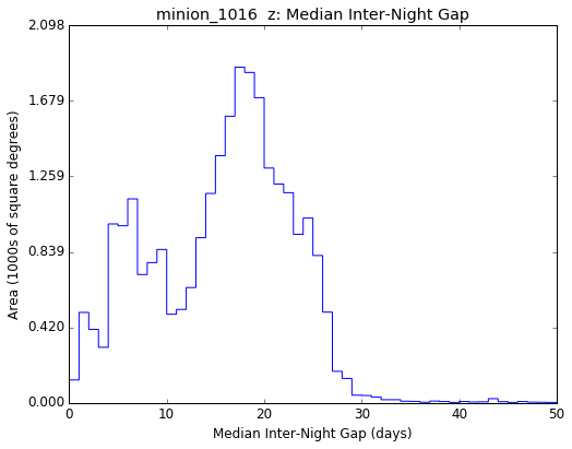
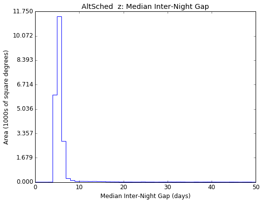
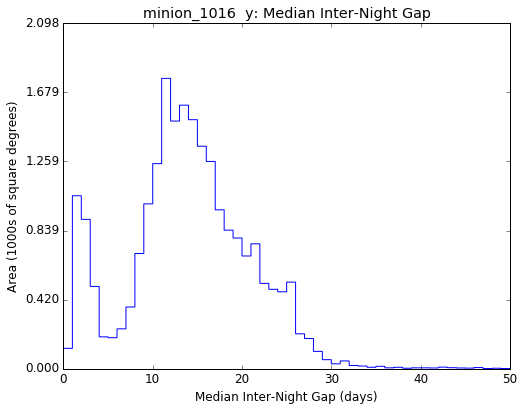
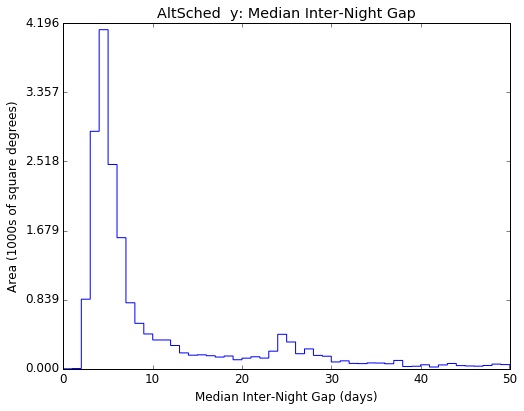
Although in this paper we advocate looking at the entire inter-night gap histogram, it is more common within LSST scheduling to present histograms of the median inter-night gap. We present these histograms in Appendix A.
So far, we have considered only the inter-night gaps between visits. However, the histogram of gaps between observations to a sky pixel within a given night is also an important metric. In order to sample transients at a large range of time-scales, both ALTSched and minion_1016 revisit each field after minutes. In addition, both schedulers carry out some number of “rapid revisits,” which are spaced less than a minute apart. minion_1016 carries out more rapid revisits than ALTSched, and the frequency can be adjusted in either scheduler by changing the field tiling density: a tiling with more overlaps between adjacent pointings yields more ~30-second revisits. We therefore omit further analysis of rapid revisits.
5 Schedulers used for other sky survey projects
The scheduling principles we describe in this paper apply to any ground-based telescope able to image a large sky area per unit time. Such telescopes include LSST (Ivezic et al., 2008), Palomar Transient Factory (PTF) (Rau et al., 2009), Zwicky Transient Facility (ZTF) (Smith et al., 2014), Pan-STARRS1 (Chambers et al., 2016), SkyMapper (Keller et al., 2007), the Dark Energy Survey (DES) (The Dark Energy Survey Collaboration, 2005), and others. Scheduling software has been developed for each of these telescopes, but often only limited information about these schedulers can be found in the literature. Broadly speaking, most schedulers are greedy algorithms like OpSim: they choose each observation as the night progresses based on where the telescope is currently pointing and on current or predicted observing conditions. In general, greedy algorithms are guaranteed to maximize merit in the long term in only the simplest of problems, and telescope scheduling is not one of those problems. To see why, consider a scenario where every field north of the telescope has a merit score of, say, 5, and every field south of the telescope has a merit score of 4. Fields directly overhead have very low merit. If the telescope happens to be pointing in the South and long slews are penalized, then a greedy algorithm will call for observing in the South the entire night, even though the globally optimal policy would be to slew to the North at the very beginning and observe there for the rest of the night.
The schedulers used for PTF (Law et al., 2009), PanSTARRS1 (Chambers & Denneau, 2008), and, as we understand it, DES (Neilsen & Annis, 2013), are all greedy algorithms. Similarly to LSST, these surveys include a wide-area component which receives multiple epochs in several bands, and we suspect that the challenges in time-domain science faced by greedy algorithms for LSST apply to these surveys as well. ZTF uses a different scheduling algorithm, which schedules an entire night at a time by solving an integer program designed to maximize observing efficiency, subject to constraints on when and how often each field needs to be observed (Bellm et al., 2019). Las Cumbres Observatory uses a similar algorithm (Saunders & Lampoudi, 2014). For LSST, this approach is challenging for a few reasons: the overhead for each observation varies considerably (a few seconds to 2 minutes); in order to achieve a more uniform sky coverage, LSST may not use fixed fields at all; and the large number of fields and observations per night may render the integer program intractable to solve repeatedly during a night when weather changes.
6 Conclusions, and Future Directions
As we have described in this article, ALTSched gives survey designers much more control over global survey characteristics than a greedy algorithm. However, certain limitations caused by our algorithm’s simplicity leave room for improvement in the more local scheduling decisions: ALTSched does not avoid taking exposures near the moon; it does not avoid poor seeing conditions or clouds; and it makes slews that are longer than necessary. These problems are not insurmountable, and because they strictly worsen ALTSched’s performance on metrics, we view these limitations optimistically as opportunities to extract even more science performance from LSST.
Between now and the beginning of full operations, the LSST Project plans to find an optimal survey strategy by running a large number of OpSim simulations, and to choose whichever yields the best compromise between science cases. We want to stress that the best survey strategy that can be found with this procedure is likely to under-perform on a number of time-domain metrics, since the parameters of OpSim don’t give much control over the survey’s cadence.
Instead, we advocate for combining the advantages of ALTSched (global schedule characteristics) with those of OpSim (sensible local scheduling decisions). We see two ways to combine forces. The simplest is to simulate surveys that switch back and forth between the two algorithms. When ALTSched tries to observe the moon, switch to a greedy algorithm that knows not to; at the end of every month, spend a day or two using a greedy algorithm to even up co-added depth across the sky; when clouds are present, use the greedy algorithm exclusively. Strategies like these should have minimal impact on the favorable properties of ALTSched, while also largely rectifying some of its limitations. Another way forward is to combine the two algorithms directly, by using a greedy scheduler whose merit function has been specifically engineered to reproduce ALTSched for large-scale decisions (which region of the sky to observe; which filter to use), but where more local scheduling decisions can be made by lower-order terms in the merit function.
In parallel, we encourage the LSST science community to continue using ALTSched as a tool to demonstrate the minimum performance that LSST is capable of. We developed most of ALTSched over a few months, and many opportunities for improvement remain: finding a scanning pattern that minimizes slew times; making more intelligent filter choices; adapting throughout the night to avoid deviating from the meridian; recovering more gracefully from downtime; using separate tilings per-filter to increase homogeneity; etc. Making improvements like these, and combining ALTSched with OpSim as described above, is what we believe will find the best survey strategy available in the limited time remaining before full operations commence.
References
- Awan et al. (2016) Awan, H., Gawiser, E., Kurczynski, P., et al. 2016, The Astrophysical Journal, 829, 50. https://doi.org/10.3847%2F0004-637x%2F829%2F1%2F50
- Bellm et al. (2019) Bellm, E., Kulkarni, S., & Graham, M. 2019, in American Astronomical Society Meeting Abstracts, Vol. 233, American Astronomical Society Meeting Abstracts #233, #363.08
- Chambers & Denneau (2008) Chambers, K. C., & Denneau, L. J. 2008, PS1 Design Reference Mission, doi:10.5281/zenodo.199860. https://doi.org/10.5281/zenodo.199860
- Chambers et al. (2016) Chambers, K. C., Magnier, E. A., Metcalfe, N., et al. 2016, ArXiv e-prints, arXiv:1612.05560
- Cowperthwaite et al. (2019) Cowperthwaite, P. S., Villar, V. A., Scolnic, D. M., & Berger, E. 2019, The Astrophysical Journal, 874, 88. https://doi.org/10.3847%2F1538-4357%2Fab07b6
- Delgado & Reuter (2016) Delgado, F., & Reuter, M. A. 2016, in Observatory Operations: Strategies, Processes, and Systems VI, Vol. 9910, International Society for Optics and Photonics, 991013
- Delgado et al. (2014) Delgado, F., Saha, A., Chandrasekharan, S., et al. 2014, in Modeling, Systems Engineering, and Project Management for Astronomy VI, Vol. 9150, International Society for Optics and Photonics, 915015
- Goldstein et al. (2018) Goldstein, D. A., Nugent, P. E., & Goobar, A. 2018, arXiv preprint arXiv:1809.10147
- Ivezic et al. (2008) Ivezic, Z., Tyson, J. A., Abel, B., et al. 2008, ArXiv e-prints, arXiv:0805.2366
- Jones et al. (2014) Jones, R. L., Yoachim, P., Chandrasekharan, S., et al. 2014, in Observatory Operations: Strategies, Processes, and Systems V, Vol. 9149, International Society for Optics and Photonics, 91490B
- Keller et al. (2007) Keller, S. C., Schmidt, B. P., Bessell, M. S., et al. 2007, PASA, 24, 1
- Law et al. (2009) Law, N. M., Kulkarni, S. R., Dekany, R. G., et al. 2009, Publications of the Astronomical Society of the Pacific, 121, 1395
- LSST Science Collaborations et al. (2017) LSST Science Collaborations, Marshall, P., Anguita, T., et al. 2017, ArXiv e-prints, arXiv:1708.04058. https://doi.org/10.5281/zenodo.842712
- Naghib et al. (2016) Naghib, E., Vanderbei, R. J., & Stubbs, C. 2016, in Proc. SPIE, Vol. 9910, Observatory Operations: Strategies, Processes, and Systems VI, 991011
- Neilsen & Annis (2013) Neilsen, E., & Annis, J. 2013, ObsTac: automated execution of Dark Energy Survey observing tactics., Tech. rep., Fermi National Accelerator Lab.(FNAL), Batavia, IL (United States)
- Rau et al. (2009) Rau, A., Kulkarni, S. R., Law, N. M., et al. 2009, PASP, 121, 1334
- Ridgway (2015) Ridgway, S. T. 2015, An Optimized Cadence for LSST: The Optimum Unit Method, Tech. Rep. 17818, LSST
- Robitaille et al. (2013) Robitaille, T. P., Tollerud, E. J., Greenfield, P., et al. 2013, Astronomy & Astrophysics, 558, A33
- Saunders & Lampoudi (2014) Saunders, E., & Lampoudi, S. 2014, in The Third Hot-wiring the Transient Universe Workshop, ed. P. R. Wozniak, M. J. Graham, A. A. Mahabal, & R. Seaman, 117–123
- Smith et al. (2014) Smith, R. M., Dekany, R. G., Bebek, C., et al. 2014, in Proc. SPIE, Vol. 9147, Ground-based and Airborne Instrumentation for Astronomy V, 914779
- The Dark Energy Survey Collaboration (2005) The Dark Energy Survey Collaboration. 2005, ArXiv Astrophysics e-prints, astro-ph/0510346
- Thomson (1904) Thomson, J. J. 1904, The London, Edinburgh, and Dublin Philosophical Magazine and Journal of Science, 7, 237
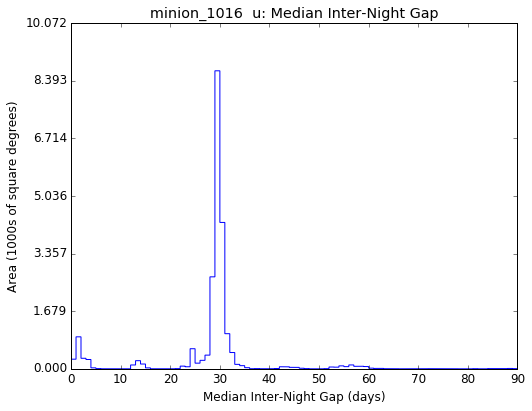
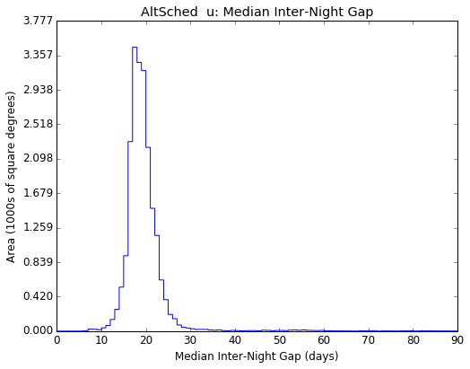
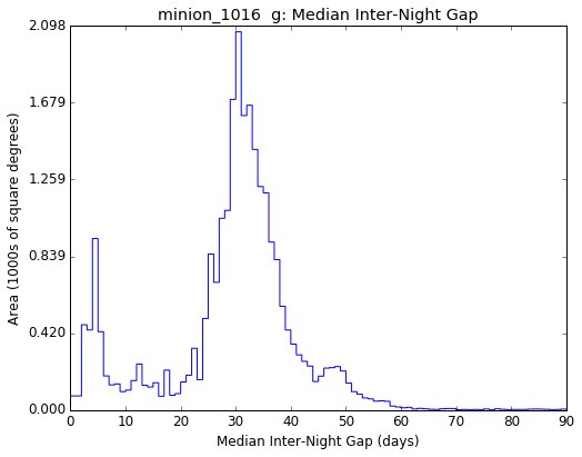
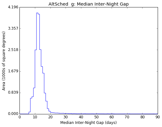
Appendix A Median Inter-Night Gaps
Here we present histograms of the median inter-night gap between consecutive visits to a sky pixel. Because minion_1016 and ALTSched have a similar total number of visits available per unit area, the mean (and therefore, roughly speaking, the median) inter-night gap should be fixed (Figure 10). We expect a two-fold reduction in the per-band median inter-night gaps (Figures 11 & 12) because ALTSched observes each field in two filters per night instead of minion_1016’s single filter.
We see additional improvement beyond these predictions because minion_1016 sometimes observes the same field more than twice per night, thus incurring additional long inter-night gaps. minion_1016 also has a slightly longer season length since it observes at a wider range of airmasses. For the u band, the improvement is actually less than twofold because both ALTSched and minion_1016 cluster observations in the u band around times with low lunar brightness.
Appendix B Inter-Night Gaps
In Figure 13, we include histograms of the typical inter-night gap between observations to a sky pixel in the , , and bands (deferred from the text).
Appendix C Uniformity Derivation
Consider a survey that observes only at pointings drawn from some fixed sky tiling. Let the area not covered by any pointing be , the area covered by exactly one pointing be , and the area covered by exactly two pointings be . Assume no part of the sky is covered by three or more fields – i.e. that the total sky area . If this tiling is observed once, the mean number of times a sky pixel will be observed is
and the RMS fluctuation in number of visits to a pixel is
If the tiling is observed times without rotation or dithering, the final average and standard deviation in number of visits will be and .
To reduce the standard deviation, we can simply rotate the tiling by some random amount each time it is observed. If we do this times, then by the central limit theorem, the probability distribution of number of visits to each sky pixel is normal with mean
and standard deviation