The Helium Abundance of NGC 6791 from Modeling of Stellar Oscillations

Abstract

The helium abundance of stars is a strong driver of evolutionary timescales, however it is difficult to measure in cool stars. We conduct an asteroseismic analysis of NGC 6791, an old, metal rich open cluster that previous studies have indicated also has a high helium abundance. The cluster was observed by Kepler and has unprecedented lightcurves for many of the red giant branch stars in the cluster. Previous asteroseismic studies with Kepler data have constrained the age through grid based modeling of the global asteroseismic parameters ($\Delta\nu$ and $\nu_{\text{max}}$). However, with the precision of Kepler data, it is possible to do detailed asteroseismology of individual mode frequencies to better constrain the stellar parameters, something that has not been done for these cluster stars as yet. In this work, we use the observed mode frequencies in 27 hydrogen shell burning red giants to better constrain initial helium abundance ($Y_{0}$) and age of the cluster. The distributions of helium abundance and age for each individual red giant are combined to create a final probability distribution for age and helium abundance of the entire cluster. We find a helium abundance of $Y_{0}=0.297\pm 0.003$ and a corresponding age of $8.2\pm 0.3$ Gyr.

1. Introduction

As the second most abundant element, helium provides valuable insight into many astrophysical situations. The helium abundance of stars has a direct link to age, such that stars evolve more quickly, and at a higher temperature and luminosity, with a larger helium abundance. This leads to a red giant branch that is hotter than one with lower helium content (Salaris et al., 2006). The study of helium can also allow us some insight into chemical evolution in the galaxy. Helium abundance is particularly difficult to measure in stars cooler than 12000 K, where the lines are very weak. Helioseismic measurements of helium abundance for the Sun (Däppen et al., 1991; Vorontsov et al., 1991; Basu & Antia, 1995, 2004), 16 Cyg (Verma et al., 2014), and HD176465 (Gai et al., 2018) are the only individual stellar measurements of helium abundance in cooler stars, although a few others have been analyzed (Verma et al., submitted).

Stellar clusters are a unique setting in which all members share the same age and composition. This enables us to study many individual stars to determine cluster properties with better precision. NGC 6791 is an old ($\sim 8$ Gyr) and metal rich ([Fe/H]$\sim+0.4$) open cluster. The combination of old age and high metallicity makes it a very interesting place to study the helium abundance. There have been many studies of the cluster and extensive work has been done to study the age of the cluster through various techniques including isochrone fitting (Harris & Canterna, 1981; Anthony-Twarog & Twarog, 1985; Stetson et al., 2003), binaries (Brogaard et al., 2011, 2012, hereafter B2012), white dwarfs (Bedin et al., 2005, 2008; García-Berro et al., 2010), and asteroseismology (Basu et al., 2011), however, not much has been done regarding helium specifically. Brogaard et al. (2011), as part of their analysis, had noted that the helium abundance of the cluster from their isochrones was likely super-solar, with a value of $Y_{0}\sim 0.30$.

Asteroseismology is a unique tool to study the interiors of stars and derive fundamental parameters, such as mass and radius, with very high precision. In conjunction with a set of reasonable stellar models, we are able to determine the properties of stars, including ages, to very high precision using the information contained in the oscillations. Thus, asteroseismic modeling of stars in clusters provides an ideal method to examine the helium abundance of the cluster in detail, especially for cool stars where traditional methods such as spectroscopy are limited.

In NGC 6791 specifically, Hekker et al. (2011a) examined the global properties of giants in the cluster, such as the mass and radius distributions, through an asteroseismic analysis of the red giants, using only the global asteroseismic parameters. By using some of the extra information contained in individual frequencies, Corsaro et al. (2012) determined the period spacing of observed modes as a way to distinguish between red clump and red giant branch stars. However, there as yet are no studies that approach the cluster by modeling the oscillations of individual stars directly.

Modeling of the individual oscillation modes in stars across the HR diagram is not a new idea, however until recently the observational data did not exist. With new space-based satellites such as CoRoT (Baglin et al., 2006) and Kepler (Borucki et al., 2010), solar-like oscillations were exposed in thousands of red giants (Hekker et al., 2009; Kallinger et al., 2010b, a; Bedding et al., 2010; Huber et al., 2010; Hekker et al., 2011b). The potential for the discovery of many more oscillating stars exists with current and forthcoming missions such as TESS (Ricker et al., 2015) and PLATO (Rauer et al., 2014). Solar-like oscillations arise in stars with outer convective layers. The oscillations are stochastically driven by the turbulent convection in the outer layers. There are several examples of asteroseismic modeling applied to main sequence stars (Miglio & Montalbán, 2005; Lebreton & Goupil, 2014; Metcalfe et al., 2014; Appourchaux et al., 2015; Roxburgh, 2016; Silva Aguirre et al., 2017; Creevey et al., 2017; White et al., 2017; Bazot et al., 2018), and recently to several red giants (Miglio et al., 2010; Pérez Hernández et al., 2016; Triana et al., 2017; Ball et al., 2018).

In this work we examine the helium abundance in NGC 6791 through two different approaches. First, we model the eclipsing binaries of B2012, taking into account a wide range of initial helium abundances in a thorough search through a fine grid of stellar evolution models. And secondly, with an asteroseismic study of the red giants in the cluster. The subgiants and main sequence stars of NGC 6791 are too faint for asteroseismic detections with Kepler. We fitted the oscillation frequencies of 27 red giants and match them to frequencies computed from stellar evolution models. Finally, we use the fact that as cluster members, all stars should have the same age and initial composition to do a joint analysis of both helium abundance and age.

The rest of our paper is organized as follows: In Section 2 we layout our target selection as well as describe the global asteroseismic parameter determination and the individual frequency fitting. In Section 3 we explain the range of parameters and choice of physics included in our models. Section!4 compares our models along the main sequence to the results obtained by B2012 and we discuss our results obtained from the red giants. We conclude with a short summary in Section 5.

2. Data & Target Selection

2.1. Eclipsing Binaries

We used the two eclipsing binary star systems in the cluster previously studied by B2012 to test our models and confirm their results. They span a large range of masses along the main sequence up to the turnoff; their properties are summarized from B2012 in Table 1. The secondary star in V20 does not have an independently measured metallicity, so we assumed [Fe/H]$=0.26$, the same as the primary. There is no asteroseismic data for these stars, however, as we shall show, the dynamical and spectroscopic parameters are sufficient to constrain the helium abundance.

Table 1Binary star parameters

	V18	V18	V20	V20
	Primary	Secondary	Primary	Secondary
Mass [$M_{\odot}$]	0.9955$\pm$0.0033	0.9293$\pm$0.0032	1.0868$\pm$0.0039	0.8276$\pm$0.0022
Radius [$R_{\odot}$]	1.1011$\pm$0.0068	0.9708$\pm$0.0089	1.397$\pm$0.013	0.7813$\pm$0.0053
Teff [K]	5600$\pm$95	5430$\pm$125	5645$\pm$95	4860$\pm$125
$[\textrm{Fe/H}]$	0.31$\pm$0.06	0.22$\pm$0.10	0.26$\pm$0.06	$\cdots$

Note. — For the purpose of fitting, the secondary of V20 was assumed to have the same metallicity as the primary component of V20

2.2. Red giant data

2.2.1 Asteroseismic data

NGC 6791 was observed for four years with the Kepler satellite, which has provided remarkable light curves for many of the stars in the field. We retrieved long cadence (30 min) light curves for Q1-Q17 from the Kepler Asteroseismic Science Operations Center (KASOC) which produces light curves and power spectra that have been processed for asteroseismology specifically (Handberg & Lund, 2014). From the red giants previously identified in the cluster (Stello et al., 2011), we chose stars with a good signal-to-noise ratio and clearly visible modes in the power spectrum. The stars chosen for this study are highlighted in Fig. 1, which shows a color-magnitude diagram of the cluster with the photometry of Stetson et al. (2003). Their global asteroseismic parameters and available spectroscopic data are listed in Table 2.2.1. We considered only stars on the red giant branch.

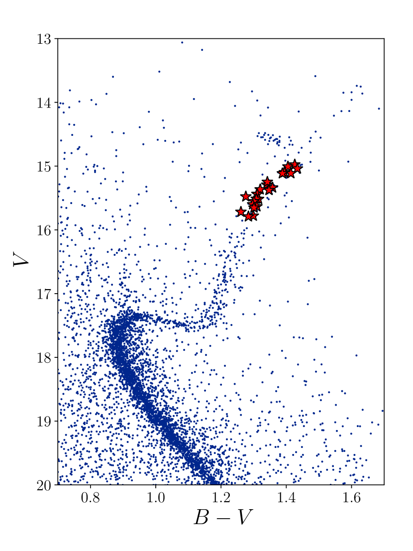
Figure 1.— Color-Magnitude Diagram of NGC 6791 with photometry of Stetson et al. (2003). Red stars denote targets studied in this work. See Table 2.2.1 for a list of their general properties.

Table 2Global asteroseismic and spectroscopic properties of target red giants.

KIC	$\nu_{\text{max}}$	$\Delta\nu$	$T_{\mathrm{eff}}$	[Fe/H]a	RVa
	$\mu\textrm{Hz}$	$\mu\textrm{Hz}$	K	dex	km/s
2436814	25.56$\pm$0.04	3.11$\pm$0.03	4289$\pm$100
2436824	34.26$\pm$0.13	3.85$\pm$0.04	4324$\pm$100
2436900	35.67$\pm$0.18	4.02$\pm$0.04	4403$\pm$78	0.40$\pm$0.02	-48.37
2436458	35.87$\pm$0.24	4.14$\pm$0.03	4340$\pm$100
2435987	36.26$\pm$0.20	4.19$\pm$0.04	4434$\pm$100	0.38$\pm$0.02	-43.75
2436097	40.53$\pm$0.22	4.54$\pm$0.04	4365$\pm$100
2437240	45.58$\pm$0.22	4.87$\pm$0.05	4440$\pm$100
2437402	46.09$\pm$0.26	4.82$\pm$0.05	4414$\pm$100
2570518	46.48$\pm$0.16	4.94$\pm$0.05	4496$\pm$71	0.38$\pm$0.02	-48.88
2569618	56.01$\pm$0.16	5.68$\pm$0.07	4479$\pm$81	0.40$\pm$0.02	-46.12
2436540	57.31$\pm$0.28	5.82$\pm$0.07	4492$\pm$83	0.41$\pm$0.02	-48.60
2436209	57.62$\pm$0.24	5.76$\pm$0.08	4498$\pm$83	0.43$\pm$0.02	-48.31
2438333	61.07$\pm$0.14	6.11$\pm$0.08	4522$\pm$80	0.43$\pm$0.02	-48.10
2438038	62.56$\pm$0.21	6.13$\pm$0.07	4450$\pm$100
2437488	65.30$\pm$0.19	6.31$\pm$0.09	4452$\pm$100
2570094	68.39$\pm$0.25	6.45$\pm$0.08	4485$\pm$100
2438140	71.37$\pm$0.24	6.72$\pm$0.10	4543$\pm$100
2437653	74.20$\pm$0.26	6.96$\pm$0.10	4588$\pm$83	0.42$\pm$0.02	-46.89
2570172	74.33$\pm$0.28	7.00$\pm$0.09	4536$\pm$85	0.44$\pm$0.02	-47.24
2436688	76.06$\pm$0.39	7.22$\pm$0.10	4537$\pm$86	0.43$\pm$0.02	-47.89
2437972	84.66$\pm$0.29	7.84$\pm$0.13	4543$\pm$100
2437781	85.15$\pm$0.29	7.74$\pm$0.16	4456$\pm$100
2437976	89.83$\pm$0.35	8.16$\pm$0.15	4525$\pm$100
2437957	92.71$\pm$0.38	8.36$\pm$0.20	4602$\pm$100
2437325	93.50$\pm$0.35	8.45$\pm$0.21	4557$\pm$100
2570244	106.31$\pm$0.33	9.17$\pm$0.27	4559$\pm$100
2437933	107.72$\pm$0.33	9.39$\pm$0.32	4610$\pm$100

As a preliminary estimate on the global asteroseismic parameters, the large separation ($\Delta\nu$) and the frequency of maximum power ($\nu_{\text{max}}$), were calculated from a 2D auto-correlation (Mosser & Appourchaux, 2009). The value of $\nu_{\text{max}}$ was further refined during our background fitting as part of the process of measuring mode frequencies. We used the diamonds code (Corsaro & De Ridder, 2014; Corsaro et al., 2015) to fit the background of the power spectrum. diamonds uses a nested sampling Monte Carlo method to efficiently arrive at a best model given a Bayesian prior. The power in the regions away from the acoustic modes can be described as a combination of three semi-Lorentzians (Kallinger et al., 2014),

$$B(\nu)=\sum\limits_{i=1}^{3}\frac{\xi\sigma_{i}^{2}/\nu_{0,i}}{1+(\nu/\nu_{0,i})^{4}}+W,$$ (1)

with the parameters $\nu_{0,i}$ representing the characteristic time scale of long-term photometric variability and granulation on two size scales, $\sigma_{i}$ is the amplitude of each of those components, $\xi$ is a normalization term of the semi-Lorentzian equal to $2\sqrt{2}/\pi$, and a white noise parameter, $W$.

The envelope of the mode excess is approximated as a Gaussian,

$$G(\nu)=H_{0}\exp{\left[-\frac{(\nu-\nu_{\rm max})^{2}}{2\sigma_{g}^{2}}\right]},$$ (2)

where $H_{0}$ is the amplitude, $\nu_{\text{max}}$ is the frequency at maximum amplitude, and $\sigma_{g}$ is the the standard deviation of the Gaussian, related to the width of the observable mode envelope. Including the Gaussian function when fitting the background ensures that the background level is accurately measured in the region of the power excess where the modes would otherwise raise the background level. The top two panels of Fig. 2 show the fitted background for two of our targets.

Individual modes frequencies were also fitted using diamonds. The methodology of using diamonds to fit red giants has been described by Corsaro et al. (2015, 2018). If a mode has a lifetime sufficiently shorter than the duration of the observations, then the mode is considered resolved and has a Lorentzian profile in the power spectrum, given as

$$P(\nu)=\frac{A^{2}/(\pi\Gamma)}{1+4/\Gamma^{2}(\nu-\nu_{0})^{2}},$$ (3)

where $A$ is the amplitude, $\nu_{0}$ is the frequency of the mode, and $\Gamma$ is the linewidth, which is inversely related to the mode lifetime.

The mode frequencies were also extracted by Corsaro et al. (2017b) for many of the targets, however, for consistency all targets were reanalyzed in this work. Very good agreement was found between both sets of frequencies. For this study we are using only the radial ($l=0$) and quadrupole ($l=2$) modes which can be treated as resolved modes. There are very few published period spacings for our target stars (Mosser et al., 2018); therefore, we chose to exclude the period spacing as an additional constraint to maintain a homogeneous data set. The bottom two panels of Fig. 2 show the results of the mode fitting process for two of our targets.

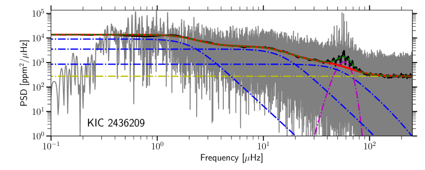
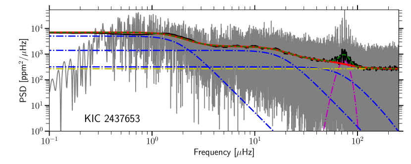
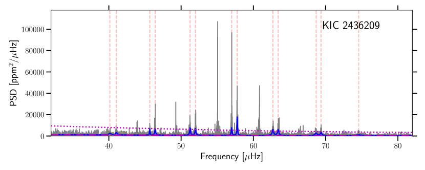
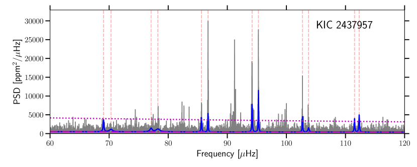
Figure 2.— Top two: Examples of the fitted background determined by diamonds. The observed power spectrum is shown in gray and a smoothed version in black. The total fitted background is shown with (green dashed line) and without (red line) the Gaussian component included. The individual components are drawn with blue (semi-Lorentzians), yellow (white noise level), and magenta (Gaussian) lines. Bottom two: Results of mode fitting for two targets. Again, the power spectrum is in gray and the fitted peaks are shown in blue. Vertical red dashed lines are placed at the locations of the central frequency of each mode. The back ground level (dashed) and eight times the background level (dotted) are both shown in magenta.

2.2.2 Spectroscopic data

Elemental diffusion in stars leads to a spread in surface metallicity along evolutionary tracks, with red giants having typically higher surface metallicity than main sequence stars in a single simple stellar population (see Fig. 7 of B2012). This can be seen in previous spectroscopic studies of the cluster. For main sequence binary stars Brogaard et al. (2011) find [Fe/H] $=0.22$–$0.34$. Boesgaard et al. (2009) measured [Fe/H] $=0.30$ in turn-off stars of the cluster. For M-giants and red giants, respectively, Origlia et al. (2006) measure [Fe/H] $=0.35$ and Carraro et al. (2006) find [Fe/H] $=0.39$. There is a clear pattern showing higher metallicity at more evolved states.

In addition, many of the stars in the cluster were observed by APOGEE (Majewski et al., 2017), a spectroscopic survey largely targeting red giants throughout the galaxy. Corsaro et al. (2017a) used APOGEE DR13 (Albareti et al., 2017) data in their analysis of granulation properties and found an average [Fe/H]=0.32. We use the spectroscopic metallicities and temperatures from DR14 (Abolfathi et al., 2018), which includes some updates to the analysis pipeline Holtzman et al. (2018), as constraints in our models. Both the radial velocities and metallicities reported by APOGEE from their ASPCAP pipeline are very homogeneous for stars in the cluster, with a mean [Fe/H]=0.41. As such, we adopt a metallicity for stars without data that is the mean metallicity of stars with APOGEE data. Temperatures, where available, were also taken from APOGEE. For stars without APOGEE data, temperatures were taken from Basu et al. (2011), where they derived $(V$ – $K)$ color-based temperatures from existing photometry.

When studying individual mode frequencies it is important to correct for the frequency shifts caused by the relative motion of the Earth around the Sun (Davies et al., 2014). While the effect is small, with high-precision data such as Kepler lightcurves, it can be on the order of your typical errorbars. For these corrections, radial velocities from APOGEE were used where available and a mean APOGEE radial velocity adopted for those without.

3. Stellar Models and Pulsation Calculations

We used the stellar evolution code Modules for Experiments in Stellar Astrophysics (MESA, v10108 Paxton et al., 2011, 2013, 2015, 2018) to create our models. We chose the abundance mixtures to be those of Grevesse & Sauval (1998). High-temperature opacities come from OPAL (Iglesias & Rogers, 1993, 1996) while low temperatures are covered by Ferguson et al. (2005). The EOS also comes from OPAL (Rogers & Nayfonov, 2002), and is the default option given in MESA (see Paxton et al. 2011 for further details). The nuclear reactions are from NACRE group (Angulo et al., 1999) and supplemented by Caughlan & Fowler (1988) with some updates to ¹²C$(\alpha,\gamma)^{16}$O (Kunz et al., 2002) and ¹⁴N$(p,\gamma)^{15}$O (Imbriani et al., 2005). The models consider convection as described by the mixing-length theory (Cox & Giuli, 1968) and the gravitational settling of elements (Thoul et al., 1994). A small amount of convective overshoot as described by Herwig (2000) was allowed during both the main sequence and red giant phases. We used the Eddington gray atmosphere approximation for the outer boundary condition.

We allowed four parameters to vary in the models we created: mass, initial [Fe/H], initial helium abundance ($Y_{0}$), and mixing-length parameter $\alpha$. The exponential convective overshoot parameter was fixed at $f_{0}=0.016$, based on the values used in the MIST isochrones (Choi et al., 2016). Initial metallicities are relative to our chosen solar abundance, with $Z/X_{\odot}=0.023$ (Grevesse & Sauval, 1998).

Two grids were computed for the cluster; the first was over a mass range of the binary stars identified in B2012 (see Table 1) and were only evolved to the onset of hydrogen shell burning. Mass points were chosen to be near the binary mass estimates. The models spanned a range in initial helium abundance of $0.26$–$0.34$. Because of the inclusion of diffusion in our models, which changes the surface metallicities, we also kept the range of initial metallicities fairly broad. The range in mixing length $\alpha$ covers 1.6 to 2.2 and encompasses our solar calibrated value of $\alpha_{\odot}=1.79$.

A second grid of models was created over the mass range of the red giants inferred from the asteroseismic scaling relations ($1.1$–$1.25$$M_{\odot}$), and with a narrower scope of parameters than the main sequence models informed by results of the binary star comparisons. All models were evolved up the red giant branch far enough to encompass the $\log g$ range of interest. Table 3 gives an overview of the range of parameters used.

Table 3Stellar model parameters

Parameter	Range	Step size
Main sequence models
$M$	0.8 $\rightarrow$ 1.12	0.003 $\rightarrow$ 0.02
$Y$	0.26 $\rightarrow$ 0.34	0.005, 0.01
Fe/H	0.15 $\rightarrow$ 0.55	0.05
$\alpha$	1.6 $\rightarrow$ 2.2	0.1
Red giant models
$M$	1.1 $\rightarrow$ 1.25	0.01
$Y$	0.28 $\rightarrow$ 0.32	0.005, 0.01
Fe/H	0.25 $\rightarrow$ 0.45	0.05
$\alpha$	1.7 $\rightarrow$ 2.1	0.1

Adiabatic mode frequencies were computed up to the Nyquist frequency for long cadence Kepler data (283 $\mu$Hz) for red giant models using GYRE (Townsend & Teitler, 2013). Frequencies were only calculated for models where $2.15<\log g<3.05$, and only for $l=0$ and $l=2$ modes. Model frequencies were corrected with the two-term surface corrections of Ball & Gizon (2014). The surface corrections of Sonoi et al. (2015) were also considered, however the resulting fits to the frequency difference showed a remaining frequency-dependent trend in the residuals. This is exemplified in Fig. 3, where we show the frequency differences between the observations and a near-optimal model for one of our targets corrected according to both Ball & Gizon (2014) and Sonoi et al. (2015).

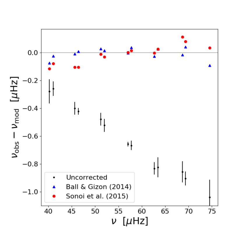
Figure 3.— The difference between the observed frequencies and model frequencies (black), Ball & Gizon (2014) corrected frequencies (blue triangles), and Sonoi et al. (2015) corrected frequencies (red circles). The errorbars are shown for the uncorrected values only. Note the frequency dependent trend left in the Sonoi et al. (2015) corrections.

The goodness of fit for each model in the grid is measured as a $\chi^{2}$ value that is a combination of individual $\chi^{2}$ values from the available observational constraints. For the binary stars,

$$\chi^{2}=\chi^{2}_{M}+\chi^{2}_{R}+\chi^{2}_{T_{\mathrm{eff}}}+\chi^{2}_{\mathrm{[Fe/H]}},$$ (4)

where only the spectroscopic temperature and metallicity, and the mass and radius from the binary analysis of B2012 were considered. For the red giants in our sample,

$$\chi^{2}=\frac{1}{3}\left(\chi^{2}_{\mathrm{ast}}+\chi^{2}_{T_{\mathrm{eff}}}+\chi^{2}_{\mathrm{[Fe/H]}}\right),$$ (5)

where the spectroscopic constraints are those from Table 2.2.1, and

$$\chi^{2}_{\mathrm{ast}}=\frac{1}{N}\sum_{i}\frac{(\nu_{\mathrm{obs},i}-\nu_{\mathrm{model},i})^{2}}{\sigma_{i}^{2}},$$ (6)

where $N$ is the total number of observed modes with an observed frequency $\nu_{\mathrm{obs}}$, and a corresponding model frequency, $\nu_{\mathrm{model}}$. For the red giants a cutoff of model $\nu_{\text{max}}$ within 3$\Delta\nu$ of the observed $\nu_{\text{max}}$ was implemented.

A probability distribution for each free parameter of the model plus age was generated and weighted appropriately by the likelihood, which is proportional to $\exp(-\chi^{2}/2)$. However, we can take advantage of the fact that these stars are all members of the same cluster and reduce the errors on our results by generating a joint probability distribution that is the product of each individual star. Furthermore, we know that the helium abundance and age are linked, so we create a 2-d probability distribution using a weighted kernel density estimator, again weighted by the likelihood.

4. Results and Discussion

4.1. Binary stars along the main sequence

We first use the binary stars of B2012 to determine the helium abundance and age of the cluster. In calculating $\chi^{2}$ for our models we assumed a [Fe/H] for the secondary of V20 that was equal to that of the primary component. We find an age of $8.5\pm 1.1$ Gyr and a $Y_{0}=0.299\pm 0.011$ from the joint probability distributions of all four stars considered. Fig. 4 shows the 2-d probability density function that was computed using weighted kernel density estimates. White and cyan contours indicate the 1-$\sigma$ and 2-$\sigma$ error ellipses, respectively. One can clearly see that there is a trend between helium abundance and age, where a higher helium abundance typically indicates a younger age.

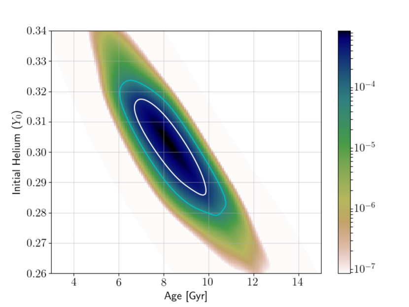
Figure 4.— Joint probability distribution of age and initial helium abundance for the two eclipsing binary systems of B2012. The 1-$\sigma$ and 2-$\sigma$ error contours are drawn in white and cyan, respectively.

For reference, B2012 determined the age to be $8.3\pm 0.3$ Gyr and $Y_{0}=0.30\pm 0.01$. Our results are entirely in agreement with B2012 and present good supporting evidence for a super-solar helium abundance in the cluster. These results also provide a check on the consistency of our giant models with previous results as the physics included in both sets of models are identical.

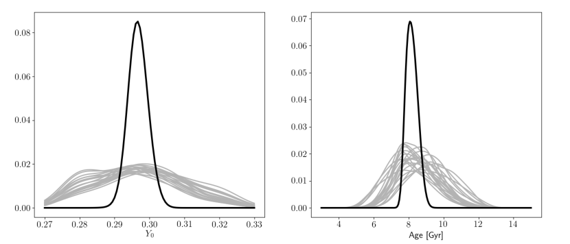
Figure 5.— One dimensional probability distributions for all targets (individual gray lines) and the combined joint probability distribution (black line) for helium abundance (left) and age (right)

4.2. Red giants

In our analysis of the red giants, we first calculated the probability density distribution of initial helium abundance and age for each red giant in the sample independently. Valle et al. (2018) noted that for a synthetic sample of cluster stars, based on the properties of NGC 6791, the estimated 1-$\sigma$ error in the age from their grid-based analysis was $\sim$1.7 Gyr, however this estimate does not to consider the sample as a complete, coeval set. As these are all members of a single star cluster, with a single age and composition, we consider the joint distribution of all stars in the sample. Fig. 5 shows these 1-d distributions of helium abundance and age, as well as the combined joint probability for the entire set of stars. We are particularly interested in the 2-d joint distribution of age and helium abundance, which can be seen in Fig. 6. The 1-$\sigma$ and 2-$\sigma$ error contours drawn in white and cyan for this distribution. For the helium abundance, we find $Y_{0}=0.297\pm 0.003$, which is compatible with the 0.30 that B2012 reported. We find an age of $8.2\pm 0.3$ Gyrs, which is, again, consistent with both the results from the analysis of the eclipsing binaries above, and the results of B2012. By using 27 individually measured stars we are able to reduce the uncertainties on the analysis significantly as compared to using only the four binary stars. This can be clearly seen in Fig. 6, where we plot the error ellipses from the previous section on top of our results.

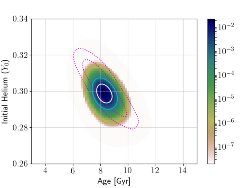
Figure 6.— Joint probability distribution of age and initial helium abundance for the for the red giants of NGC 6791. The 1-$\sigma$ and 2-$\sigma$ error contours are drawn in white and cyan, respectively. The error contours from the binary analysis (Fig. 4) are shown in magenta dotted lines.

There are not many studies that have looked at the helium abundance specifically, however, there are many to determine the age. Table 2 of Wu et al. (2014a) summarizes the literature on NGC 6791 very well. To put our values in the context of previous literature we have plotted our values of helium abundance and age against many of the published literature values in Fig. 7. Most of the values come from isochrone fitting to various photometric observations, where the isochrones assumed either a given $\Delta Y/\Delta Z$ relation, or a fixed $Y$ in a few cases. The earlier studies (Harris & Canterna, 1981; Anthony-Twarog & Twarog, 1985; Kaluzny, 1990) had metallicities near the solar value and were largely dominated by either Yale isochrones (Ciardullo & Demarque, 1977) or those of Vandenberg (1983, 1985), which found drastically different ages between 6 and 12 Gyrs.

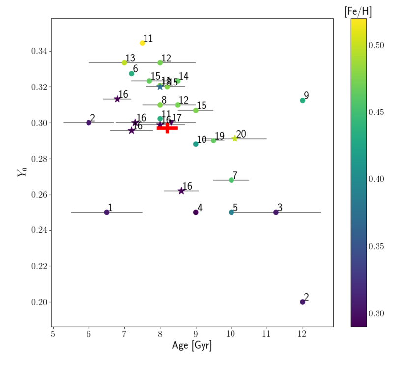
Figure 7.— Comparison of literature values for age and helium abundance used to derive given age. Our results are shown as the red cross where the width and height are indicative of the size of the error. Each published value is colored by the metallicity. Different symbols reflect the method used to obtain the result: isochrones (circles), binary stars (triangles), and asteroseismology (stars). Numbers correspond to the following references: ¹Harris & Canterna (1981), ²Anthony-Twarog & Twarog (1985), ³Kaluzny (1990), ⁴Garnavich et al. (1994), ⁵Montgomery et al. (1994), ⁶Kaluzny & Rucinski (1995), ⁷Tripicco et al. (1995), ⁸Chaboyer et al. (1999), ⁹Stetson et al. (2003), ¹⁰King et al. (2005), ¹¹Carney et al. (2005), ¹²Carraro et al. (2006), ¹³Anthony-Twarog et al. (2007), ¹⁴Kalirai et al. (2007), ¹⁵Grundahl et al. (2008), ¹⁶Basu et al. (2011), ¹⁷Brogaard et al. (2012), ¹⁸Wu et al. (2014b), ¹⁹An et al. (2015), ²⁰Kallinger et al. (2018).

More recent work by Carney et al. (2005); Carraro et al. (2006); Kalirai et al. (2007) and (Anthony-Twarog et al., 2007), which had metallicities closer to [Fe/H] $\sim$ +0.4, all found relatively consistent ages within the range of 7–9 Gyrs, no matter the choice of isochrone. All of these studies had helium abundances that were fixed by their chosen $\Delta Y/\Delta Z$ relation, and were near the high end ($Y_{0}>0.30$) of helium abundances found in the literature.

With global asteroseismic results, Basu et al. (2011) found ages in the range of 6.8 to 8.6 Gyrs from several different sets of isochrones, with a typical error of 0.5 Gyrs. Two of their sets of models were computed for the same set of isochrones (YREC, Demarque et al., 2008) with a higher helium abundance of $Y_{0}=0.30$, and a regular value of $Y_{0}=0.26$. The difference in helium abundance had the effect of reducing the age by 1.3 Gyrs in the higher helium models. However, our age result agrees more strongly with the lower helium abundance model. Using the $Y^{2}$ isochrones (Demarque et al., 2004) instead, Basu et al. (2011) find an age of 8.0$\pm$0.7 Gyrs for a helium abundance of $Y_{0}\sim 0.30$, which is in excellent agreement with our work. In contrast to the asteroseismic-based results of Basu et al. (2011), recent work by Kallinger et al. (2018) determined an age of the cluster using similar grid-based asteroseismic methods that was significantly larger ($10.1\pm 0.9$ Gyr) using their non-linear corrections to the scaling relations. An age of 10.1 Gyrs is inconsistent with our joint analysis of all the cluster stars.

Our analysis also enables us to derive a mean mass of red giant stars of $\overline{M}_{RGB}=1.15\pm 0.01$. Basu et al. (2011) found a mean mass of red giants of 1.20$\pm$0.01$M_{\odot}$ and Miglio et al. (2012) reported $\overline{M}_{RGB}=1.23\pm 0.02$. Miglio et al. (2012) applied a small correction to $\Delta\nu$ in their analysis before computing masses, however both of these values are significantly higher than our value. This can be partially attributed to our analysis covering a smaller portion of the red giant branch; our analysis covers $\log g\sim 2.4$–3.0, while both Basu et al. (2011) and Miglio et al. (2012) use stars further up the giant branch with a lower $\log g$ limit of $\sim$2.1. However, part of the difference can also come from the use of the asteroseismic scaling relations, which have been noted to need some form of a correction (White et al., 2011; Gaulme et al., 2016) to both $\Delta\nu$ and $\nu_{\text{max}}$ (Viani et al., 2017). Kallinger et al. (2018) derived non-linear corrections to the scaling laws, and estimated the mean mass of ascending red giant branch stars to be $1.10\pm 0.03$$M_{\odot}$ for NGC 6791. This is also in slight disagreement with our value, likely because of the choice of scaling correction applied, but closer than the uncorrected asteroseismic values. The deviations can partially be attributed to the assumption that $\Delta\nu$ follows only a first-order asymptotic expression, which leads to the need for corrections. A summary of several different corrections to the scaling laws, and their applicability in the context of red giants in eclipsing binaries, can be found in Gaulme et al. (2016) and Brogaard et al. (2018a). Most of the corrections are empirical in nature, but recent work by Ong & Basu (2019) show physical motivation for deriving a better estimator of $\Delta\nu$ from stellar models.

In B2012, they determined a mass of the lower RGB stars to be $1.15\pm.02$ from their analysis of the main sequence binary stars and chosen isochrones. This value is consistent with our results. A blue straggler system in NGC 6791 was modeled by Brogaard et al. (2018b), who determined the initial masses of the two components. The component who donated mass to the companion during its red giant phase began its life with a mass of 1.15 $M_{\odot}$, which agrees well with the mean mass of red giants that we studied.

We have assumed here that the NGC 6791 is a single-aged stellar population–a valid assumption for open clusters given the evidence so far (Bragaglia et al., 2014; Cunha et al., 2015; Villanova et al., 2018). Globular clusters, on the other hand, have been shown to have multiple stellar populations (Bastian & Lardo, 2018, and references therein). The ability to detect and distinguish the multiple populations within globular clusters through asteroseismology could provide some possible insight into the formation and evolution of such clusters, however, the data to do such an analysis at the level of precision required is currently lacking. The K2 mission observed more that 20 clusters, both globular and open (Dotson et al., 2018), however the length of observations is much shorter ($\sim$80 days) than what we have for NGC 6791, and thus the frequency resolution of modes will be worse. There is an opportunity here for TESS (near the continuous viewing zone) or PLATO observations to provide the data needed for such a project.

5. Conclusions

It is important to study the helium abundance of stars because it is a significant driver of stellar evolution. Although it is not possible to directly measure the helium abundance through spectroscopy in cool stars, asteroseismology provides a valuable method for studying the helium abundance through the modeling of stellar oscillations.

In this paper we presented our work on the asteroseismic modeling of red giants in NGC 6791. We looked at the initial helium abundance and age through stellar models and theoretical oscillation frequencies of those models. By using the information contained in the frequencies of 27 red giant stars we were able to determine the age of NGC 6791 to a higher precision than just using global oscillation properties. In addition, the joint analysis of all stars allows us to present the most precise measures of age and helium abundance for the cluster thus far.

We first modeled two binary star systems in the cluster and find $Y_{0}=0.299\pm 0.011$ and an age of $8.5\pm 1.1$ Gyr. We then fitted observed mode frequencies and matched them to theoretical frequencies from a large grid of stellar evolution models. From this we find an initial helium abundance $Y_{0}=0.297\pm 0.003$ and an age of $8.2\pm 0.3$ Gyr. The ages we find are consistent with several of the several of the recent literature values that used isochrones with helium abundances around 0.30. Finally, we determined the mean mass of first ascent red giant branch stars to be $1.15\pm 0.008$$M_{\odot}$.

Future observations from missions such as TESS, PLATO, and Gaia (Gaia Collaboration et al., 2016, 2018) will provide further data, potentially from other clusters, for which we can do these types of studies. Information from Gaia, such as luminosity, is quite complementary to the lightcurves commonly used in asteroseismic analyses. There is much potential for deeper study, in particular, of the helium abundance, beyond what has been done here. An in-depth look at all the mode frequencies can reveal information about acoustic glitches and provide constraints on the depth of the helium ionization zone for evolved stars (Broomhall et al., 2014, and references therein). Additionally, the methods of mean density inversions have been extended to more evolved stars, which allows for the further exploitation of information contained in the oscillations (Buldgen et al., 2019).

References

- Abolfathi et al. (2018) Abolfathi, B., Aguado, D. S., Aguilar, G., et al. 2018, The Astrophysical Journal Supplement Series, 235, 42
- Albareti et al. (2017) Albareti, F. D., Allende Prieto, C., Almeida, A., et al. 2017, ApJS, 233, 25
- An et al. (2015) An, D., Terndrup, D. M., Pinsonneault, M. H., & Lee, J.-W. 2015, ApJ, 811, 46
- Angulo et al. (1999) Angulo, C., Arnould, M., Rayet, M., et al. 1999, Nucl. Phys. A, 656, 3
- Anthony-Twarog & Twarog (1985) Anthony-Twarog, B. J., & Twarog, B. A. 1985, ApJ, 291, 595
- Anthony-Twarog et al. (2007) Anthony-Twarog, B. J., Twarog, B. A., & Mayer, L. 2007, AJ, 133, 1585
- Appourchaux et al. (2015) Appourchaux, T., Antia, H. M., Ball, W., et al. 2015, A&A, 582, A25
- Baglin et al. (2006) Baglin, A., Auvergne, M., Barge, P., et al. 2006, in ESA Special Publication, Vol. 1306, The CoRoT Mission Pre-Launch Status - Stellar Seismology and Planet Finding, ed. M. Fridlund, A. Baglin, J. Lochard, & L. Conroy, 33
- Ball & Gizon (2014) Ball, W. H., & Gizon, L. 2014, A&A, 568, A123
- Ball et al. (2018) Ball, W. H., Themeßl, N., & Hekker, S. 2018, MNRAS, 478, 4697
- Bastian & Lardo (2018) Bastian, N., & Lardo, C. 2018, Annual Review of Astronomy and Astrophysics, 56, 83
- Basu & Antia (1995) Basu, S., & Antia, H. M. 1995, MNRAS, 276, 1402
- Basu & Antia (2004) —. 2004, ApJ, 606, L85
- Basu et al. (2011) Basu, S., Grundahl, F., Stello, D., et al. 2011, ApJ, 729, L10
- Bazot et al. (2018) Bazot, M., Creevey, O., Christensen-Dalsgaard, J., & Meléndez, J. 2018, A&A, 619, A172
- Bedding et al. (2010) Bedding, T. R., Huber, D., Stello, D., et al. 2010, ApJ, 713, L176
- Bedin et al. (2008) Bedin, L. R., King, I. R., Anderson, J., et al. 2008, ApJ, 678, 1279
- Bedin et al. (2005) Bedin, L. R., Salaris, M., Piotto, G., et al. 2005, ApJ, 624, L45
- Boesgaard et al. (2009) Boesgaard, A. M., Jensen, E. E. C., & Deliyannis, C. P. 2009, AJ, 137, 4949
- Borucki et al. (2010) Borucki, W. J., Koch, D., Basri, G., et al. 2010, Science, 327, 977
- Bragaglia et al. (2014) Bragaglia, A., Sneden, C., Carretta, E., et al. 2014, ApJ, 796, 68
- Brogaard et al. (2011) Brogaard, K., Bruntt, H., Grundahl, F., et al. 2011, A&A, 525, A2
- Brogaard et al. (2012) Brogaard, K., VandenBerg, D. A., Bruntt, H., et al. 2012, A&A, 543, A106
- Brogaard et al. (2018a) Brogaard, K., Hansen, C. J., Miglio, A., et al. 2018a, MNRAS, 476, 3729
- Brogaard et al. (2018b) Brogaard, K., Christiansen, S. M., Grundahl, F., et al. 2018b, MNRAS, 481, 5062
- Broomhall et al. (2014) Broomhall, A. M., Miglio, A., Montalbán, J., et al. 2014, MNRAS, 440, 1828
- Buldgen et al. (2019) Buldgen, G., Rendle, B., Sonoi, T., et al. 2019, MNRAS, 482, 2305
- Carney et al. (2005) Carney, B. W., Lee, J.-W., & Dodson, B. 2005, AJ, 129, 656
- Carraro et al. (2006) Carraro, G., Villanova, S., Demarque, P., et al. 2006, ApJ, 643, 1151
- Caughlan & Fowler (1988) Caughlan, G. R., & Fowler, W. A. 1988, Atomic Data and Nuclear Data Tables, 40, 283
- Chaboyer et al. (1999) Chaboyer, B., Green, E. M., & Liebert, J. 1999, AJ, 117, 1360
- Choi et al. (2016) Choi, J., Dotter, A., Conroy, C., et al. 2016, ApJ, 823, 102
- Ciardullo & Demarque (1977) Ciardullo, R. B., & Demarque, P. 1977, Transactions of the Astronomical Observatory of Yale University, 33, 1
- Corsaro & De Ridder (2014) Corsaro, E., & De Ridder, J. 2014, A&A, 571, A71
- Corsaro et al. (2015) Corsaro, E., De Ridder, J., & García, R. A. 2015, A&A, 579, A83
- Corsaro et al. (2018) —. 2018, A&A, 612, C2
- Corsaro et al. (2012) Corsaro, E., Stello, D., Huber, D., et al. 2012, ApJ, 757, 190
- Corsaro et al. (2017a) Corsaro, E., Mathur, S., García, R. A., et al. 2017a, A&A, 605, A3
- Corsaro et al. (2017b) Corsaro, E., Lee, Y.-N., García, R. A., et al. 2017b, Nature Astronomy, 1, 0064
- Cox & Giuli (1968) Cox, J. P., & Giuli, R. T. 1968, Principles of stellar structure
- Creevey et al. (2017) Creevey, O. L., Metcalfe, T. S., Schultheis, M., et al. 2017, A&A, 601, A67
- Cunha et al. (2015) Cunha, K., Smith, V. V., Johnson, J. A., et al. 2015, ApJ, 798, L41
- Däppen et al. (1991) Däppen, W., Gough, D. O., Kosovichev, A. G., & Thompson, M. J. 1991, A New Inversion for the Hydrostatic Stratification of the Sun, ed. D. Gough & J. Toomre, 111
- Davies et al. (2014) Davies, G. R., Handberg, R., Miglio, A., et al. 2014, MNRAS, 445, L94
- Demarque et al. (2008) Demarque, P., Guenther, D. B., Li, L. H., Mazumdar, A., & Straka, C. W. 2008, Ap&SS, 316, 31
- Demarque et al. (2004) Demarque, P., Woo, J.-H., Kim, Y.-C., & Yi, S. K. 2004, The Astrophysical Journal Supplement Series, 155, 667
- Dotson et al. (2018) Dotson, J., Barentsen, G., & Cody, A. M. 2018, in American Astronomical Society Meeting Abstracts, Vol. 231, American Astronomical Society Meeting Abstracts #231, 413.06
- Ferguson et al. (2005) Ferguson, J. W., Alexander, D. R., Allard, F., et al. 2005, ApJ, 623, 585
- Gai et al. (2018) Gai, N., Basu, S., & Tang, Y. 2018, ApJ, 856, 123
- Gaia Collaboration et al. (2016) Gaia Collaboration, Prusti, T., de Bruijne, J. H. J., et al. 2016, A&A, 595, A1
- Gaia Collaboration et al. (2018) Gaia Collaboration, Brown, A. G. A., Vallenari, A., et al. 2018, A&A, 616, A1
- García-Berro et al. (2010) García-Berro, E., Torres, S., Althaus, L. G., et al. 2010, Nature, 465, 194
- Garnavich et al. (1994) Garnavich, P. M., Vandenberg, D. A., Zurek, D. R., & Hesser, J. E. 1994, AJ, 107, 1097
- Gaulme et al. (2016) Gaulme, P., McKeever, J., Jackiewicz, J., et al. 2016, ApJ, 832, 121
- Grevesse & Sauval (1998) Grevesse, N., & Sauval, A. J. 1998, Space Sci. Rev., 85, 161
- Grundahl et al. (2008) Grundahl, F., Clausen, J. V., Hardis, S., & Frandsen, S. 2008, A&A, 492, 171
- Handberg & Lund (2014) Handberg, R., & Lund, M. N. 2014, MNRAS, 445, 2698
- Harris & Canterna (1981) Harris, W. E., & Canterna, R. 1981, AJ, 86, 1332
- Hekker et al. (2009) Hekker, S., Kallinger, T., Baudin, F., et al. 2009, A&A, 506, 465
- Hekker et al. (2011a) Hekker, S., Basu, S., Stello, D., et al. 2011a, A&A, 530, A100
- Hekker et al. (2011b) Hekker, S., Gilliland, R. L., Elsworth, Y., et al. 2011b, MNRAS, 414, 2594
- Herwig (2000) Herwig, F. 2000, A&A, 360, 952
- Holtzman et al. (2018) Holtzman, J. A., Hasselquist, S., Shetrone, M., et al. 2018, AJ, 156, 125
- Huber et al. (2010) Huber, D., Bedding, T. R., Stello, D., et al. 2010, ApJ, 723, 1607
- Iglesias & Rogers (1993) Iglesias, C. A., & Rogers, F. J. 1993, ApJ, 412, 752
- Iglesias & Rogers (1996) —. 1996, ApJ, 464, 943
- Imbriani et al. (2005) Imbriani, G., Costantini, H., Formicola, A., et al. 2005, European Physical Journal A, 25, 455
- Kalirai et al. (2007) Kalirai, J. S., Bergeron, P., Hansen, B. M. S., et al. 2007, ApJ, 671, 748
- Kallinger et al. (2018) Kallinger, T., Beck, P. G., Stello, D., & Garcia, R. A. 2018, A&A, 616, A104
- Kallinger et al. (2010a) Kallinger, T., Mosser, B., Hekker, S., et al. 2010a, A&A, 522, A1
- Kallinger et al. (2010b) Kallinger, T., Weiss, W. W., Barban, C., et al. 2010b, A&A, 509, A77
- Kallinger et al. (2014) Kallinger, T., De Ridder, J., Hekker, S., et al. 2014, A&A, 570, A41
- Kaluzny (1990) Kaluzny, J. 1990, MNRAS, 243, 492
- Kaluzny & Rucinski (1995) Kaluzny, J., & Rucinski, S. M. 1995, Astronomy and Astrophysics Supplement Series, 114, 1
- King et al. (2005) King, I. R., Bedin, L. R., Piotto, G., Cassisi, S., & Anderson, J. 2005, AJ, 130, 626
- Kunz et al. (2002) Kunz, R., Fey, M., Jaeger, M., et al. 2002, ApJ, 567, 643
- Lebreton & Goupil (2014) Lebreton, Y., & Goupil, M. J. 2014, A&A, 569, A21
- Majewski et al. (2017) Majewski, S. R., Schiavon, R. P., Frinchaboy, P. M., et al. 2017, AJ, 154, 94
- Metcalfe et al. (2014) Metcalfe, T. S., Creevey, O. L., Doğan, G., et al. 2014, The Astrophysical Journal Supplement Series, 214, 27
- Miglio & Montalbán (2005) Miglio, A., & Montalbán, J. 2005, A&A, 441, 615
- Miglio et al. (2010) Miglio, A., Montalbán, J., Carrier, F., et al. 2010, A&A, 520, L6
- Miglio et al. (2012) Miglio, A., Brogaard, K., Stello, D., et al. 2012, MNRAS, 419, 2077
- Montgomery et al. (1994) Montgomery, K. A., Janes, K. A., & Phelps, R. L. 1994, AJ, 108, 585
- Mosser & Appourchaux (2009) Mosser, B., & Appourchaux, T. 2009, A&A, 508, 877
- Mosser et al. (2018) Mosser, B., Gehan, C., Belkacem, K., et al. 2018, A&A, 618, A109
- Ong & Basu (2019) Ong, J. M. J., & Basu, S. 2019, ApJ, 870, 41
- Origlia et al. (2006) Origlia, L., Valenti, E., Rich, R. M., & Ferraro, F. R. 2006, ApJ, 646, 499
- Paxton et al. (2011) Paxton, B., Bildsten, L., Dotter, A., et al. 2011, The Astrophysical Journal Supplement Series, 192, 3
- Paxton et al. (2013) Paxton, B., Cantiello, M., Arras, P., et al. 2013, The Astrophysical Journal Supplement Series, 208, 4
- Paxton et al. (2015) Paxton, B., Marchant, P., Schwab, J., et al. 2015, The Astrophysical Journal Supplement Series, 220, 15
- Paxton et al. (2018) Paxton, B., Schwab, J., Bauer, E. B., et al. 2018, The Astrophysical Journal Supplement Series, 234, 34
- Pérez Hernández et al. (2016) Pérez Hernández, F., García, R. A., Corsaro, E., Triana, S. A., & De Ridder, J. 2016, A&A, 591, A99
- Rauer et al. (2014) Rauer, H., Catala, C., Aerts, C., et al. 2014, Experimental Astronomy, 38, 249
- Ricker et al. (2015) Ricker, G. R., Winn, J. N., Vanderspek, R., et al. 2015, Journal of Astronomical Telescopes, Instruments, and Systems, 1, 014003
- Rogers & Nayfonov (2002) Rogers, F. J., & Nayfonov, A. 2002, ApJ, 576, 1064
- Roxburgh (2016) Roxburgh, I. W. 2016, A&A, 585, A63
- Salaris et al. (2006) Salaris, M., Weiss, A., Ferguson, J. W., & Fusilier, D. J. 2006, ApJ, 645, 1131
- Silva Aguirre et al. (2017) Silva Aguirre, V., Lund, M. N., Antia, H. M., et al. 2017, ApJ, 835, 173
- Sonoi et al. (2015) Sonoi, T., Samadi, R., Belkacem, K., et al. 2015, A&A, 583, A112
- Stello et al. (2011) Stello, D., Meibom, S., Gilliland, R. L., et al. 2011, ApJ, 739, 13
- Stetson et al. (2003) Stetson, P. B., Bruntt, H., & Grundahl, F. 2003, Publications of the Astronomical Society of the Pacific, 115, 413
- Thoul et al. (1994) Thoul, A. A., Bahcall, J. N., & Loeb, A. 1994, ApJ, 421, 828
- Townsend & Teitler (2013) Townsend, R. H. D., & Teitler, S. A. 2013, MNRAS, 435, 3406
- Triana et al. (2017) Triana, S. A., Corsaro, E., De Ridder, J., et al. 2017, A&A, 602, A62
- Tripicco et al. (1995) Tripicco, M. J., Bell, R. A., Dorman, B., & Hufnagel, B. 1995, AJ, 109, 1697
- Valle et al. (2018) Valle, G., Dell’Omodarme, M., Tognelli, E., Prada Moroni, P. G., & Degl’Innocenti, S. 2018, A&A, 619, A158
- Vandenberg (1983) Vandenberg, D. A. 1983, The Astrophysical Journal Supplement Series, 51, 29
- Vandenberg (1985) —. 1985, The Astrophysical Journal Supplement Series, 58, 711
- Verma et al. (2014) Verma, K., Faria, J. P., Antia, H. M., et al. 2014, ApJ, 790, 138
- Viani et al. (2017) Viani, L. S., Basu, S., Chaplin, W. J., Davies, G. R., & Elsworth, Y. 2017, ApJ, 843, 11
- Villanova et al. (2018) Villanova, S., Carraro, G., Geisler, D., Monaco, L., & Assmann, P. 2018, ApJ, 867, 34
- Vorontsov et al. (1991) Vorontsov, S. V., Baturin, V. A., & Pamiatnykh, A. A. 1991, Nature, 349, 49
- White et al. (2011) White, T. R., Bedding, T. R., Stello, D., et al. 2011, ApJ, 743, 161
- White et al. (2017) White, T. R., Benomar, O., Silva Aguirre, V., et al. 2017, A&A, 601, A82
- Wu et al. (2014a) Wu, T., Li, Y., & Hekker, S. 2014a, ApJ, 786, 10
- Wu et al. (2014b) —. 2014b, ApJ, 781, 44