LHC Constraints on a Mediator Coupled to Heavy Quarks

Manuel Drees, Zhongyi Zhang

Physikalisches Institut and Bethe Center for Theoretical Physics,
Bonn University, 53115 Bonn, Germany

We apply LHC data to constrain a simplified extension of the Standard Model containing a new spin$-1$ mediator $R$, which does not couple to first generation quarks, and a spinor dark matter particle $\chi$. We recast ATLAS and CMS searches for final states containing one or more jet(s) + $\not{E}_{T}$, with or without $b$ tags, as well as searches for di–jet resonances with $b$ or $t$ tagging. We find that LHC constraints on the axial vector couplings of the mediator are always stronger than the unitarity bound, which scales like $m_{R}/m_{t}$. If $R$ has a sizable invisible branching ratio, the strongest LHC bound on both vector couplings and axial vector coupling comes from a di–jet + $\not{E}_{T}$ search with or without double $b$ tag. These bounds are quite strong for $m_{R}<1$ TeV, even though we have switched off all couplings to valence quarks. Searches for a di–jet resonance with double $b$ tag lead to comparable bounds with the previous results even if $R\rightarrow\chi\bar{\chi}$ decays are allowed; these are the only sensitive LHC searches if the invisible branching ratio of $R$ is very small or zero.

1 Introduction

Simplified models of particle dark matter often need a mediator coupling the dark matter particle $\chi$ to some particles in the Standard Model (SM). Models where the mediator couples to both quarks and leptons are strongly constrained by LHC searches for $\ell^{+}\ell^{-}$ resonances, where $\ell$ stands for a charged lepton [1, 2, 3, 4]. This motivates the investigation of “leptophobic” models, where the mediator does not couple to leptons. In case of a spin$-1$ mediator $R$, universal couplings to all quarks are often assumed. If $R$ has a sizable branching ratio into invisible final states, which is generally true if $m_{R}>2m_{\chi}$, the allowed vector and axial vector couplings are then strongly constrained by mono–jet searches [5, 6] unless $m_{R}$ is well above $1$ TeV. For mediator mass between $1$ and $2.5$ TeV, searches for di–jet resonances [7, 8] perform even better. Additionally, the constraints from spin–dependent and spin–independent interactions in direct detection experiments imposes strong constraints on couplings to first generation quarks [9]; these bounds scale like $m_{R}$.

In our previous study [10], which applies LEP data to probe the low $m_{R}$ region, we therefore switched off all couplings to first generation quarks and axial vector couplings to second generation quarks in order to avoid an excess in direct Dark Matter detection experiments. At tree level, axial vector couplings lead to spin–dependent contributions to the scattering cross section, which also receive a sizable contribution from strange quarks, whereas vector couplings lead to spin–independent contributions which only probe $u$ and $d$ quarks in the nucleon [11]. In our model the scattering on nuclei can therefore only proceed via loop diagrams, and should thus be strongly suppressed. Moreover, the non–zero couplings to other quarks are still available to generate a sizable annihilation rate to explain the observed dark matter relic density through thermal freeze–out. By switching off couplings to first generation quarks, and hence to all valence quarks, we greatly reduce the cross sections for $pp$ scattering processes with an $R$ boson in the intermediate or final state. The published bounds from the LHC experiments, which assume equal couplings of $R$ to all quarks, are therefore no longer valid.

The goal of this article is to estimate the LHC constraints on this model. We showed in ref.[10] that LEP data impose strong constraints only for $m_{R}<10$ GeV, and become entirely insensitive for $m_{R}>70$ GeV. Here we therefore focus on scenarios with $m_{R}\geq 10$ GeV. The relevant searches we exploit are similar to those that constrain scenarios with flavor–universal couplings of $R$: mono–jet + $\not{E}_{T}$ searches, di–jet + $\not{E}_{T}$ searches and di–jet resonance searches. By switching off couplings to light quarks, we increase the branching ratio for $R\rightarrow b\bar{b}$ or $t\bar{t}$ decays. Since in background events most jets originate from light quarks or gluons, $b$ or $t$ tagging can increase the signal to background ratio even for flavor–universal couplings of $R$, and should be even more helpful in our case.

The reminder of this article is organized as follows. In Sec. 2, we briefly describe the Lagrangian of the simplified model containing a leptophobic mediator, which does not couple to first generation quarks. The application to the relevant LHC data is discussed in Sec. 3. The LEP result and the tightest unitarity condition from top quark are compared to the LHC exclusion limits we estimate. Finally, Sec. 4 contains our summary and conclusions.

2 The Simplified Model

2.1 Lagrangian and Free Parameters

A spinor dark sector particle (DSP) and a new spin$-1$ mediator connecting DSP to SM particles are introduced to extend the SM. Therefore the total Lagrangian is given by:

$$\mathcal{L}=\mathcal{L}_{\rm SM}+\mathcal{L}_{\rm DSP}+\mathcal{L}_{R}+\mathcal{L}_{I}\,.$$ (1)

Since we use MadGraph [12] to generate the Monte Carlo Events, the kinetic terms in the Lagrangian follow the default convention in MadGraph. The mediator part of the Lagrangian is thus:

$$\mathcal{L}_{R}=-\frac{1}{4}F^{\mu\nu}F_{\mu\nu}-\frac{1}{2}m_{R}^{2}R^{\mu}R_{\mu}\,,\ \ \ {\rm with}\ F_{\mu\nu}\equiv\partial_{\mu}R_{\nu}-\partial_{\nu}R_{\mu}\,.$$ (2)

In order to allow both vector and axial-vector couplings the DSP should be a Dirac fermion, because Majorana fermions cannot have a vector interaction. Again using MadGraph convention, the corresponding piece of the Lagrangian is

$$\mathcal{L}_{\rm DSP}=\bar{\chi}(i\not{\partial}-m_{\chi})\chi\,.$$ (3)

Finally, the interaction terms are

$$\mathcal{L}_{I}=\sum_{q=s,\,c}g^{V}_{q}R_{\mu}\bar{q}\gamma^{\mu}q+\sum_{q=b,\,t}R_{\mu}\bar{q}\gamma^{\mu}\left(g^{V}_{q}-g^{A}_{q}\gamma^{5}\right)q+R_{\mu}\bar{\chi}\gamma^{\mu}\left(g^{V}_{\chi}-g^{A}_{\chi}\gamma^{5}\right)\chi\,.$$ (4)

In this model DSPs can scatter off nucleons via $R$ exchange. The corresponding spin–independent and spin–dependent cross sections are to leading order in perturbation theory [9]:

$$\sigma_{n/p}^{\rm SD}=a_{n/p}^{2}\frac{3\mu^{2}_{n/p}}{\pi m_{R}^{4}}\,;\ \ \sigma_{n/p}^{\rm SI}=f_{n/p}^{2}\frac{3\mu^{2}_{n/p}}{\pi m_{R}^{4}}\,;\ \ \mu_{n/p}=\frac{m_{\chi}m_{n/p}}{m_{\chi}+m_{n/p}}\,.$$ (5)

The coefficients $a_{n/p}$ and $f_{n/p}$ depend on different combinations of couplings:

$$f_{p}=g_{\chi}^{V}(2g_{u}^{V}+g_{d}^{V})\,;\ \ f_{n}=g_{\chi}^{V}(g_{u}^{V}+2g_{d}^{V})\,;$$ (6)

and [13]

$$a_{n/p} = g^{A}_{\chi}\sum_{q=u,\,d,\,s}\Delta q^{(n/p)}g_{q}^{A}\,;$$

$$\Delta u^{(p)} = \Delta d^{(n)}=0.84\pm 0.02\,;$$ (7)

$$\Delta u^{(n)} = \Delta d^{(p)}=-0.43\pm 0.02\,;$$

$$\Delta s^{(p)} = \Delta s^{(n)}=-0.09\pm 0.02\,.$$

Eqs.(6) show that setting $g^{V}_{u,\,d}=0$ suffices to make the leading order spin–independent cross sections on protons and neutrons vanish. On the other hand, eqs.(2.1) show that $g^{A}_{u,\,d,\,s}=0$ is needed in order to “switch off” the leading order spin–dependent cross sections; weak $SU(2)$ invariance then implies $g^{A}_{c}=0$ as well.

This leaves us with seven free parameters: $g^{V}_{s,\,c}$, $g^{V}_{b,\,t}$, $g^{A}_{b,\,t}$, $g^{A}_{\chi}$, $g^{V}_{\chi}$, $m_{R}$ and $m_{\chi}$. However, since $R$ does not couple to leptons signals involving missing transverse energy $\not{E}_{T}$ require a pair of DSPs in the final state. Since SM $Z$ boson couple to all quarks, final states with an $R$ boson replaced by an invisible decaying $Z$ boson will always contribute to (and indeed often dominate) the background to these signals. Clearly the signal can only compete with this background from on–shell $Z$ bosons if on–shell $R\rightarrow\chi\bar{\chi}$ decays are possible. The relevant quantity is then the branching ratio for these decays, rather than the couplings $g^{V}_{\chi}$ and $g^{A}_{\chi}$ separately. Moreover, the DSP mass $m_{\chi}$ also affects the signal only through this branching ratio. This observation implies that replacing the Dirac DSP $\chi$ by a complex scalar $\phi$ is trivial, since again only the branching ratio for $R\rightarrow\phi\bar{\phi}$ decays is relevant in that model.

Turning to quark couplings, we assume all non–vanishing couplings to be equal. In case of axial vector couplings, this can again be motivated by $SU(2)$ invariance. This would still allow different, non–vanishing second and third generation vector couplings, but we set them equal for simplicity. Note that the case $g^{V}_{s}=g^{V}_{c}=0$ would give very similar results as the scenario with non–vanishing axial vector couplings. The reason is that contributions to the relevant matrix elements from $g^{V}_{q}$ and $g^{A}_{q}$ differ only by terms of the order $m_{q}/Q$, where $Q$ is the energy scale of the process. Since the parton distribution function for top quarks is still very small at the energies we are interested in, and top tagging turns out to be quite inefficient, the relevant quark is the $b$ quark, and $m_{b}/Q\ll 1$ for all cases of interest to us. The main difference between vector and axial vector couplings is therefore that in the former case couplings to second generation quarks are included, while these couplings vanish in the latter case.

Finally we are therefore left with four relevant free parameters: $g^{V}_{q}$, $g^{A}_{q}$, ${\rm Br}(R\rightarrow\chi\bar{\chi})$ and $m_{R}$. Since the parton distribution functions for second generation quarks in the proton are significantly larger than those for third generation (basically, $b$) quarks, for fixed size of the non–vanishing couplings we expect much smaller total cross sections for the case $g_{q}^{V}=0,\,g_{q}^{A}\equiv g_{q}$ than for the case $g_{q}^{A}=0,\,g_{q}^{V}\equiv g_{q}$. On the other hand, scenarios with $g^{V}=0$ should have higher efficiency for $b$ tagging, which is required in some searches.

2.2 Perturbativity and Unitarity Conditions

We will use leading order tree–level diagrams in the simulation. Therefore, the relevant couplings should not be too big, so that the perturbation theory is reliable. We impose the simple perturbativity condition

$$\Gamma_{R}<m_{R}\,,$$ (8)

where $\Gamma_{R}$ is the total decay width of the mediator. The partial width for $R\rightarrow f\bar{f}$ decay, where $f$ is some fermion, is:

$$\Gamma(R\rightarrow f\bar{f})=\frac{m_{R}N_{C}^{f}}{12\pi}\sqrt{1-4z_{f}}\left[(g^{V}_{f})^{2}+(g^{A}_{f})^{2}+z_{f}\left(2(g^{V}_{f})^{2}-4(g^{A}_{f})^{2}\right)\right]\,,$$ (9)

where $z_{f}\equiv m_{f}^{2}/m_{R}^{2}$ and $N_{C}^{f}=3\ (1)$ for $f=q\ (f=\chi)$. Since we use ${\rm Br}(R\rightarrow\chi\bar{\chi})$ as free parameter instead of $m_{\chi}$ and $g_{\chi}^{V,A}$, the perturbativity condition can be written as

$$\sum_{q}\sqrt{1-4z_{q}}\left[(g^{V}_{q})^{2}+(g^{A}_{q})^{2}+z_{q}\left(2(g^{V}_{q})^{2}-4(g^{A}_{q})^{2}\right)\right]<4\pi[1-{\rm Br}(R\rightarrow\chi\bar{\chi})]<4\pi\,.$$ (10)

In the next section, we will only discuss the mass range where the bounds for vector or axial vector couplings are smaller than $2$; this satisfies the perturbativity condition.

Another important theoretical constraint on the parameters in the Lagrangian originates from demanding that unitarity in scattering amplitudes is preserved [14]. This constraints the axial vector couplings between the mediator and fermions:

$$g_{f}^{A}\frac{m_{f}}{m_{R}}\leqslant\sqrt{\frac{\pi}{2}}\,.$$ (11)

Due to the assumption of universal axial vector couplings to $b$ and $t$ quarks, the strongest constraint always comes from the much heavier top, and becomes quite strong for light mediator:

$$g_{q}^{A}\leqslant\sqrt{\frac{\pi}{2}}\frac{m_{R}}{m_{t}}=\frac{m_{R}}{137.59\ {\rm GeV}}\,.$$ (12)

For example, for $m_{R}=10$ GeV, $g^{A}$ should be smaller than $0.08$. In contrast, for $m_{R}>275$ GeV the unitarity constraint becomes weaker than the perturbativity condition.

3 Application to LHC Data

In this section, we recast various LHC searches to constrain the model introduced in section 2, including a mono–jet + $\not{E}_{T}$ search [6], multi–jet + $\not{E}_{T}$ searches [15, 16, 17], a multi–jet + $\not{E}_{T}$ searches with $t$ tag [18], a multi–jet + $\not{E}_{T}$ search with double $b$ tag [19], and di–jet resonance searches with final state $b$–jets [20] or $t$–jets [21].

In order to simulate the events and recast the analysis, we use FeynRules [22] to encode the model and generate an UFO file [23] for the simulator, MadGraph [12] to generate the parton level events, PYTHIA 8 [24] for QCD showering and hadronization, DELPHES [25] to simulate the ATLAS and CMS detectors, and CheckMATE [26, 27] to reconstruct and $b$–tag jets, to calculate kinematic variables, and to apply cuts. We note that the toolkit CheckMATE uses a number of additional tools for phenomenology research [28, 29, 30, 31, 32, 33, 34, 35, 36, 37, 38].

Let us first discuss final states involving missing $E_{T}$. These are often categorized as “mono–jet + $\not{E}_{T}$” and “multi–jet + $\not{E}_{T}$” final states. However, the “mono–jet” searches also allow the presence of at least one additional jet. On the other hand, “multi–jet” searches do indeed require at least two jets in the final state. These signals thus overlap, but are not identical to each other.

As remarked in the Introduction, missing $E_{T}$ in signal events always comes from invisibly decaying mediators, $R\rightarrow\chi\bar{\chi}$. Since multi–jet searches require at least two jets in the final state, we use MadGraph to generate parton–level events with a $\chi\bar{\chi}$ pair plus one or two partons (quarks or gluons) in the final state. The former process only gets contributions from the left diagram in fig. 1 plus its crossed versions, including the contribution from $gq\rightarrow Rq$. Note that $R$ has to couple to the initial quark line in this case. We use parton distribution functions (PDFs) with five massless flavors; the mass of the corresponding quarks should be set to $0$ in order to avoid the inconsistency with massless evolution equations (DGLAP equations). The $b-$quark PDF is nonzero, but it is still considerably smaller than those of first generation quarks. The contribution from this diagram, which is formally of leading order in $\alpha_{S}$, is therefore quite small, especially for scenarios with $g^{V}_{q}=0$ where $R$ only couples to third generation quarks.

If we allow the final state to contain two partons in addition to the DSPs, there are contributions with only light quarks or gluons in the initial state; an example is shown in the middle of fig. 1, but there are several others. These diagrams are higher order in $\alpha_{S}$, but they receive contributions from initial states with much larger PDFs than those contributing to the first diagram. It is thus not clear a priori which of these contributions will be dominant for a given set of cuts.

There is one additional complication. At the parton level, events with one and two partons in the final state are clearly distinct. However, once we include QCD showering, which is handled automatically by PYTHIA, the distinction becomes less clear. In particular, a single parton event with an additional gluon from showering can no longer be distinguished from a certain two parton event without additional gluon. Naively adding contributions with one and two partons in the final state before showering can therefore lead to double counting. Similarly, if one of the final–state quarks shown in the middle diagram of fig. 1 has small $p_{T}$, the diagram can be approximated by $g\rightarrow q\bar{q}$ splitting followed by $gq\rightarrow Rq$ production. This contribution is already contained in the crossed version of the left diagram of fig. 1, via the scale–dependent PDF of $q$, so simply adding these diagrams again leads to double counting. MadGraph avoids both kinds of double counting by using the “MLM matching” algorithm [39]. Of course, showering can add more than one additional parton; indeed, we find significant rates for final states with up to four jets (having transverse energy $E_{T}\geq 35$ GeV each).

Figure 1: Examples of Feynman diagrams contributing to mono–jet + $\not{E}_{T}$ (left), di–jet + $\not{E}_{T}$ (center) and di–jet resonance (right) final states; in the former two cases it is assumed that the mediator $R$ decays into two dark sector particles, which escape detection, whereas in the latter case $R$ is assumed to decay into a quark antiquark pair. The diagram to the right is unique (with different initial states contributing), and the one on the left is unique up to crossing; however, many additional diagrams, with different combinations of partons in the initial and final states and different propagators, contribute to $R+$di–jet production.

Searches for final states leading to large missing $E_{T}$ are typical cut–and–count analyses, where the final state is defined by cuts on the type and number of final state objects (in particular, leptons and jets with or without $b-$tag) and on kinematic quantities (in particular, the transverse momenta or energies of the jets and the missing $E_{T}$). The experiments themselves designed these cuts, and estimated the expected number of surviving SM background events. The comparison with the actually observed number of events after cuts then allows to derive upper bounds on the number of possible signal events. We pass our simulated signal events through CheckMATE, which applies the same cuts (including detector resolution effects), and compares the results with the upper bounds obtained by the experiments.

The second kind of search we consider are searches for di–jet resonances. The leading–order signal diagram is shown on the right in fig. 1. In this case the final state contains no partons besides the mediator $R$; for $g^{V}_{q}=0$, only $b\bar{b}$ initial states contribute, whereas for non–vanishing vector couplings also $s\bar{s}$ and $c\bar{c}$ initial states contribute. Of course, the left and middle diagrams shown in fig. 1 also contribute to this signal if $R$ decays into a $q\bar{q}$ pair. However, in this case one has to add two powers of $\alpha_{S}$ in order to access initial states including only light quarks or gluons. Moreover, if all final state transverse momenta are small, which maximizes the cross section, the contribution from the middle diagram is actually already included in the right diagram, via double $g\rightarrow q\bar{q}$ splitting. The left and middle diagrams should therefore only be included in inclusive $R$ production when a full NLO or even NNLO calculation is performed, which is beyond the scope of this work.

Note also that resonance searches are not cut–and–count analyses. The analyses still use a set of basic acceptance cuts, in this case on the (pseudo–)rapidities and transverse momenta of the two leading jets. The bound on resonance production is then obtained by fitting a smooth function to the di–jet invariance mass distribution, which is assumed to be dominated by backgrounds, and computing the limit on a possible additional contribution peaked at a certain value (basically, the mass of the resonance). The current version of CheckMATE does not include comparison with this kind of searches. However, CheckMATE does allow to estimate the efficiency with which our signal events pass the acceptance cuts. This allows to derive the constraints from resonance searches on our model, as follows.

The most sensitive di–jet resonance search we found is that of ref. [20], which requires a double $b-$tag in the final state. This paper presents the resulting upper bounds for a couple of models. One of them is quite similar to ours, but assumes universal couplings to all quarks; this leads to a greatly enhanced resonance production cross section, and a somewhat reduced branching ratio into $b\bar{b}$ pairs, compared to our model. The paper also gives the cut efficiency for the model with universal couplings. We, therefore, recast their cuts and compare the cut efficiencies of their model and our models in order to estimate the bound for our model through the following rescaling:

$$\sigma_{\rm max,\,ours}=\sigma_{\rm max,\,exp}\cdot\frac{\epsilon_{\rm exp}}{\epsilon_{\rm ours}}\,.$$ (13)

Here $\sigma_{\rm max,\,ours}$ is the largest allowed cross section for our model, $\sigma_{\rm max,\,exp}$ is the largest allowed cross section in the original experimental analysis, $\epsilon_{\rm exp}$ is the selection efficiency of the model in the paper, and $\epsilon_{\rm ours}$ is the selection efficiency of our model.

Finally, we cannot easily reproduce the top tagging required in the di–top resonance search [21]. However, even if we assume $100\%$ efficiency for the di–top tag, the resulting bound is much weaker than our recast of [20] described in the previous paragraphs. We therefore do not show this bound in our summary plot.

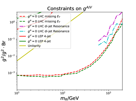
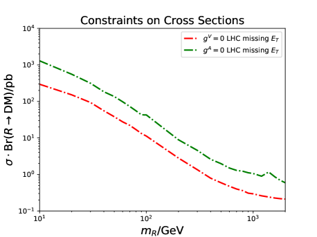
Figure 2: The left frame shows the bound on the squared coupling of the mediator to quarks times the relevant branching ratio of the mediator that we derive by recasting various LHC bounds (dashed and dot–dashed curves). The lower solid curve shows the unitarity bound (12) on the axial vector coupling, and the thin solid lines in the top–left corner show constraints from recast LEP constraints [10] based on analyses by the ALEPH collaboration. For $g^{A}=0$ only vector couplings $g^{V}_{q}$ are allowed with $q=s,c,b,t$, while for $g^{V}=0$ only axial vector couplings $g_{q}^{A}$ are allowed with $q=b,t$. LHC missing $E_{T}$ results are from the combination of mono–jet and multi–jet analyses. The right frame shows the upper bound on the total cross sections from the missing $E_{T}$ analyses.

The results of our analyses are summarized in fig. 2. The thin solid lines in the top–left corner show the bounds we derived [10] from analyses of older ALEPH searches for four jet final states at the $e^{+}e^{-}$ collider LEP; note that these bounds are valid for $m_{R}<2m_{\chi}$. The solid straight line is the unitarity bound (12) applied to the top mass; recall that it applies only to axial vector couplings. (Since top quarks could not be produced at the LEP collider, in [10] we only considered the unitarity constraints involving $m_{b}$ and $m_{\chi}$.)

The other results shown in fig. 2 are new. The dashed curves show the bounds on the square of the coupling of $R$ to quarks times the branching ratio for invisible $R$ decays which we derived from the most sensitive jet(s) plus missing $E_{T}$ searches, for pure axial vector couplings (red, upper curve) and pure vector couplings (green, lower curve); the right frame shows the corresponding bounds on the signal cross section, defined as the total cross section for the on–shell production of a mediator $R$ times the invisible branching ratio of $R$. It is important to note that these constraints are only significant in our model if on–shell $R\rightarrow\chi\bar{\chi}$ decays are allowed, i.e. they constrain a region of parameter space that is complementary to that analyzed in ref. [10].

The dot–dashed curves in the left frame show the bounds on the square of the coupling of $R$ to quarks times the branching ratio for $R\rightarrow q\bar{q}$ decays that result from searches for di–jet resonances, again separately for pure axial vector couplings (purple, upper curve) and pure vector couplings (blue, lower curve). The relevant analysis by the ATLAS collaboration [20] is sensitive only to $m_{R}\geq 600$ GeV.

The difference between the constraints on vector and axial vector couplings is almost entirely due to the additional coupling to $s$ and $c$ quarks that we allow only for the former, as discussed in Sec. 2.1. In particular, we see that the constraint from the $b\bar{b}$ resonance search is much stronger for the model with vector couplings.

In the left frame of Fig. 2 the curves depicting the bounds from searches for final states containing $\not{E}_{T}$ evidently lie below the ones showing bounds from di–jet resonance searches, except for the scenario with pure vector coupling at $m_{R}\simeq 2$ TeV. However, this is somewhat misleading, since the dashed curves show bounds on $g_{q}^{2}\cdot{\rm Br}(R\rightarrow\chi\bar{\chi})$, while the dot–dashed curves shows bounds on $g_{q}^{2}\cdot[1-Br(R\rightarrow\chi\bar{\chi})]$. For $m_{R}\geq 1$ TeV the two sets of constraints on the coupling are actually comparable if ${\rm Br}(R\rightarrow\chi\bar{\chi})\simeq 0.3\ (0.1)$, for pure vector (axial vector) coupling; for even smaller invisible branching ratio of $R$, the $b\bar{b}$ resonance search imposes the stronger constraint in this large $m_{R}$ region. We note that for $m_{R}^{2}\gg m_{t}^{2}$ and $g_{\chi}=g_{q}$, i.e. equal coupling of the mediator to the DSP and to heavy quarks, the invisible branching ratio of $R$ is below $1/7\ (1/13)$ for pure axial vector (vector) coupling, the difference being due to the different number of accessible $q\bar{q}$ final states.

Within the missing $E_{T}$ searches the best bound on $g^{V}_{q}$ for $m_{R}<1.4$ TeV is from ref.[19], a double $b$ tagged multi–jet + $\not{E}_{T}$ analysis, while ref.[15], a general multi–jet + $\not{E}_{T}$ analysis, is the most sensitive one for $m_{R}\geq 1.4$ TeV; this change of the most sensitive analysis explains the structure in the dark green curves at that $m_{R}$, which is most visible in the right frame. In contrast, the strongest bound on $g^{A}_{q}$ is always from ref.[19] with double $b$ tag, which also determines the bound on the vector coupling for $m_{R}<1.4$ TeV. This explains why the bound on the coupling is actually very similar in both cases: the required double $b$ tag means that the contribution from partonic events containing only $s$ or $c$ quarks, which only exists in the case of vector coupling, has very small efficiency, since the $b$ tag requirement can only be satisfied though mistagging, or through additional $b$ quarks produced in hard showering. As a result the bound on the total cross section, shown in the right frame, is much weaker for pure vector coupling, since the coupling to $s$ and $c$ quarks greatly increases the total cross section while contributing little to the most sensitive signal.

We also consider multi–jet analyses specially designed for final states containing two top quarks [16, 18]. However, the top–tag in [18] is not easy to recast directly. We therefore, assume $100\%$ efficiency to reach the most ideal bound. Unfortunately, even this ideal bound on $g^{2}$ is $10$ times weaker than that from the analysis which only requires a double $b$-tag. One reason is that both $b\bar{b}$ and $t\bar{t}$ final states may lead to $b$-tagged jets, while the selection rules specially designed for top jets exclude the $b\bar{b}$ final state. Moreover, for our assumption of equal couplings the cross section for $t\bar{t}R$ production is considerably smaller than that for $b\bar{b}R$ production.

As noted above, we also derived constraints on our model from mono–jet searches. The most sensitive analysis has been published in [6], and does not require any flavor tagging. The resulting constraint on the vector coupling is only slightly weaker than that shown in Fig. 2, while the constraint on the axial vector coupling is not competitive. Since no flavor tagging is required, the large contribution from $s$ or $c$ quarks in the initial and final states has similar efficiency as contributions with $b$ quarks, and greatly strengthens the limit on the vector coupling.

Before concluding this section, we comment on loop processes that allow $gg$ initial states to contribute to our signals. The relevant Feynman diagrams are shown in Fig. 3. They involve two additional QCD vertices relative to the leading–order $R+$jet production channels, i.e. they are formally NNLO. Nevertheless the large gluon flux in the proton might lead to sizable contributions. We again use FeynRules and Madgraph to simulate these events at the parton level.

Figure 3: Loop diagrams contributing to $R+$jet production from gluon fusion.

Note that the tree–level contributions we discussed so far are only sensitive to the absolute value of the couplings of the mediator to quarks. In contrast, in the loop diagrams all quark flavors contribute coherently, so the relative signs between different $Rq\bar{q}$ couplings are important.

Let us first consider pure vector couplings. Here our simplified model as written is well–behaved also at QCD one–loop level. We find that the loop contributions of Fig. 3 only contribute at most $2\%$ of the leading–order mono–jet signal if all $g^{V}_{q}$ are set equal; this contribution is reduced by another factor of $5$ if we instead take $g^{V}_{s/b}=-g^{V}_{c/t}$. In particular, there is no enhancement for small $m_{R}$; instead, the cross section after cuts approaches a constant once $m_{R}\ll p_{T,{\rm cut}}$. Recall also that in this case there are tree–level contributions involving the strange quark content of the proton, which is much larger than that of $b$ quarks (although still considerably smaller than that of gluons). We can thus always safely neglect these loop contributions for non–zero vector couplings.

In contrast, in case of non–vanishing axial vector couplings our model with equal couplings of the mediator to all heavy quarks leads to a $ggR$ anomaly, i.e. this version of our simplified model is not well–behaved at the 1–loop level. We therefore took $g^{A}_{b}=-g^{A}_{t}$ in order to cancel this anomaly.

Moreover, the loop amplitude now receives a contribution that scales $\propto 1/m_{R}$. As a result, for $m_{R}=10$ GeV the loop contribution to the mono–jet cross section exceeds the tree–level contribution by about a factor of $20$. We find that nevertheless the best bound still comes from the final state with two $b-$jets and missing $E_{T}$. Recall that here $gg$ initial states are accessible already at tree–level. Since in the loop diagrams the external gluon has to be virtual, so that it can split into a $b\bar{b}$ pair, the loop contribution is still NNLO relative to this tree–level contribution. Nevertheless the $1/m_{R}$ enhancement, which is associated with heavy (i.e. top) quark loops, means that including the loop diagram with $g^{A}_{b}=-g^{A}_{t}$ would tighten the upper limit on the squared coupling shown in Fig. 2 at $m_{R}=10$ by about $40\%$. For $m_{R}=50$ GeV, however, the loop contribution only doubles the total mono–jet signal, and the final bound on the squared coupling from the di-$b$ final state is improved by about $3\%$.

It should be clear that setting $g^{A}_{b}=-g^{A}_{t}$ is only one solution to cancel the anomaly. Another possibility is to introduce a very heavy quark $Q$ satisfying $g^{A}_{Q}=-2g^{A}_{b}=-2g^{A}_{t}$. This would lead to even larger loop contributions for small $m_{R}$; however, the unitarity bound (12) would then also have to be applied to $m_{Q}$, and might even supersede the LHC constraint.

In sum, we conclude that for axial vector couplings loop corrections involving two–gluon initial states might moderately strengthen the LHC constraint for $m_{R}<50$ GeV, the exact result depending on the UV completion of the model. Note also that this source of loop corrections adds incoherently to the signal, i.e. it cannot weaken the bounds presented in Fig. 2. We therefore believe that this Figure, which is independent of the UV completion, is a better representation of the LHC constraints on our model.

4 Conclusions

In this study, we discuss a model containing a Dirac fermion $\chi$ as dark matter candidate as well as a spin$-1$ mediator $R$. We assume that $R$ has vanishing couplings to first generation quarks and vanishing axial vector coupling to second generation quarks, thereby easily satisfying constraints from direct dark matter searches. By assuming vanishing couplings to leptons the otherwise most sensitive LHC searches, based on analyses of $\ell^{+}\ell^{-}$ final states where $\ell$ stands for a charged lepton, are evaded as well. Due to the vanishing couplings to light quarks, and hence to all valence quarks in the proton, the $R$ production rate at the LHC is considerably smaller than for the more commonly considered scenarios with (essentially) universal couplings to all quarks.

Nevertheless LHC data impose quite strong constraints on the model if the branching ratio for invisible $R$ decays is sizable, which requires $m_{R}>2m_{\chi}$. The best LHC bound then always comes from searches for final states containing jets plus missing $E_{T}$. Our CheckMATE–based recast of these analyses leads to an upper bound on the product of the squared coupling and the invisible branching ratio of $R$ of $10^{-3}$ for $m_{R}\leq 200$ GeV. This weakens to $0.01$ ($1$) for $m_{R}=600$ GeV ($2$ TeV), see Fig. 2. Searches for invisibly decaying mediators have traditionally been framed as “mono–jet” searches (which allow additional jets in the final state, as mentioned above), and have been interpreted assuming equal (vector or axial vector) couplings to all quarks [5, 6]. For pure axial vector couplings these bounds are actually weaker than ours if $m_{R}\leq 600$ GeV. Since the signal need only contain a single hard jet, and no $b-$tagging is used, one needs a very strong cut on the missing $E_{T}$ to suppress the background; for $m_{R}\>\raisebox{-2.15277pt}{$\stackrel{{\scriptstyle\textstyle<}}{{\sim}}$}\>1$ TeV this leads to a much worse cut efficiency than the most sensitive analysis we use, which requires two tagged $b-$jets plus missing $E_{T}$. For $m_{R}\>\raisebox{-2.15277pt}{$\stackrel{{\scriptstyle\textstyle<}}{{\sim}}$}\>600$ GeV this search may thus also impose tighter bounds on the model with universal couplings. Nevertheless the bound on $g_{q}^{2}$ times the invisible branching ratio from mono–jet searches in the model with universal coupling becomes significantly stronger than ours for larger $m_{R}$, by about one order of magnitude for $m_{R}=1.5$ TeV.

For $m_{R}\geq 0.6$ TeV roughly comparable bounds on the product of the squared coupling and the branching ratio of $R$ into $q\bar{q}$ quarks can be derived from an ATLAS search for $b\bar{b}$ resonances. Searches for generic di–jet or $t\bar{t}$ resonances yield much weaker constraints on our model. Generic di–jet resonance searches at the 13 TeV LHC become sensitive only at a resonance mass above 1.5 TeV or so. The resulting bounds on mediators with unsuppressed couplings to valence quarks are quite strong. For example, for $m_{R}=1.5$ TeV the ATLAS analysis [7] gives a bound on the squared universal coupling to quarks in a leptophobic model that is about two orders of magnitude stronger than our bound from $b\bar{b}$ resonant searches in the model with vector couplings, which in turn is a factor of about $3$ stronger than the analogous bound in the model with axial vector couplings.

We thus see that both in the missing $E_{T}$ and in the resonance searches switching off the couplings to first generation quarks greatly weakens the limits on the couplings for $m_{R}>1$ TeV, less so for smaller mediator masses.

Since the energy scale of these reactions (e.g. the missing $E_{T}$, or $m_{R}$ in the resonance searches) is much larger than the masses of the relevant quarks, the matrix elements for vector and axial vector couplings are almost the same. Unless $m_{R}\gg m_{\chi}$ for equal coupling strengths the branching ratio for invisible $R\rightarrow\chi\bar{\chi}$ decays will be larger for pure vector coupling than for pure axial vector coupling; however, this effect is absorbed by interpreting the relevant constraints as upper bounds on the product of the squared coupling times the invisible branching ratio, as we did in the above discussion.

LHC searches lose sensitivity to our model if $m_{R}>2$ TeV, or if $m_{R}<0.6$ TeV and $m_{R}<2m_{\chi}$. Probing significantly higher values of $m_{R}$ would require higher center–of–mass energies; since all relevant searches are background–limited, increasing the luminosity will increase the reach only slowly. If on–shell $R\rightarrow\chi\bar{\chi}$ decays are not possible, missing $E_{T}$ searches at the LHC are essentially hopeless in our model. The reason is that in this case a signal which is of second order in the couplings of the mediator has to compete with SM signals that are first order in electroweak couplings, in particular the production of $Z$ and $W$ bosons which decay into neutrinos. For $m_{R}<70$ GeV the old LEP experiments have some sensitivity, but the resulting bound is not very strong [10]. Straightforward di–jet resonance searches at the LHC are not possible for $m_{R}$ much below $0.6$ TeV, since the trigger rate would be too high. One might consider previous hadron colliders, in particular the Tevatron. However, these earlier colliders were $p\bar{p}$ colliders, where the $b\bar{b}$ background includes contributions where both initial–state quarks are valence quarks; recall that in our model the signal does not receive contributions from such initial states.

A probably more promising approach is to consider final states containing an additional hard “tagging jet” besides the mediator $R$. Both ATLAS [40] and CMS [41] have presented bounds on rather light di–jet resonances using this trick, which is also employed in the “mono–jet” searches. Unfortunately these searches are currently not easy to recast, since they use “fat jet” substructure techniques. In any case, in order to gain sensitivity to our model this technique would probably have to be combined with $b-$tagging, which proved crucial for deriving useful constraints from di–jet resonance searches at $m_{R}>600$ GeV. An analysis of this kind should be able to probe deep into the parameter space with $m_{R}<600$ GeV and $m_{R}<2m_{\chi}$.

ACKNOWLEDGEMENTS

This work was partially supported by the by the German ministry for scientific research (BMBF).

References

- [1] Vardan Khachatryan et al. Search for heavy resonances decaying to tau lepton pairs in proton-proton collisions at TeV. JHEP, 02:048, 2017.
- [2] Morad Aaboud et al. Search for new high-mass phenomena in the dilepton final state using 36 fb???1 of proton-proton collision data at TeV with the ATLAS detector. JHEP, 10:182, 2017.
- [3] Morad Aaboud et al. Search for additional heavy neutral Higgs and gauge bosons in the ditau final state produced in 36 fb???1 of pp collisions at TeV with the ATLAS detector. JHEP, 01:055, 2018.
- [4] Albert M Sirunyan et al. Search for high-mass resonances in dilepton final states in proton-proton collisions at 13 TeV. JHEP, 06:120, 2018.
- [5] Albert M Sirunyan et al. Search for dark matter produced with an energetic jet or a hadronically decaying W or Z boson at TeV. JHEP, 07:014, 2017.
- [6] Morad Aaboud et al. Search for dark matter and other new phenomena in events with an energetic jet and large missing transverse momentum using the ATLAS detector. JHEP, 01:126, 2018.
- [7] Morad Aaboud et al. Search for new phenomena in dijet events using 37 fb-1 of collision data collected at 13 TeV with the ATLAS detector. Phys. Rev., D96(5):052004, 2017.
- [8] Albert M Sirunyan et al. Search for dijet resonances in proton-proton collisions at = 13 TeV and constraints on dark matter and other models. Phys. Lett., B769:520–542, 2017. [Erratum: Phys. Lett.B772,882(2017)].
- [9] Mads T. Frandsen, Felix Kahlhoefer, Anthony Preston, Subir Sarkar, and Kai Schmidt-Hoberg. LHC and Tevatron Bounds on the Dark Matter Direct Detection Cross-Section for Vector Mediators. JHEP, 07:123, 2012.
- [10] Manuel Drees and Zhongyi Zhang. Constraints on a Light Leptophobic Mediator from LEP Data. JHEP, 08:194, 2018.
- [11] John R. Ellis and Ricardo A. Flores. Elastic supersymmetric relic - nucleus scattering revisited. Phys. Lett., B263:259–266, 1991.
- [12] Johan Alwall, Michel Herquet, Fabio Maltoni, Olivier Mattelaer, and Tim Stelzer. Madgraph 5: going beyond. Journal of High Energy Physics, 2011(6):1–40, 2011.
- [13] C. Patrignani et al. Review of Particle Physics. Chin. Phys., C40(10):100001, 2016.
- [14] Felix Kahlhoefer, Kai Schmidt-Hoberg, Thomas Schwetz, and Stefan Vogl. Implications of unitarity and gauge invariance for simplified dark matter models. JHEP, 02:016, 2016.
- [15] Morad Aaboud et al. Search for squarks and gluinos in final states with jets and missing transverse momentum using 36 fb -1 of TeV pp collision data with the ATLAS detector. Phys. Rev., D97(11):112001, 2018.
- [16] Morad Aaboud et al. Search for a scalar partner of the top quark in the jets plus missing transverse momentum final state at =13 TeV with the ATLAS detector. JHEP, 12:085, 2017.
- [17] The ATLAS collaboration. Search for squarks and gluinos in events with an isolated lepton, jets and missing transverse momentum at = 13 TeV with the ATLAS detector. 2016.
- [18] Morad Aaboud et al. Search for large missing transverse momentum in association with one top-quark in proton-proton collisions at = 13 TeV with the ATLAS detector. JHEP, 05:041, 2019.
- [19] Morad Aaboud et al. Search for supersymmetry in events with -tagged jets and missing transverse momentum in collisions at TeV with the ATLAS detector. JHEP, 11:195, 2017.
- [20] Morad Aaboud et al. Search for resonances in the mass distribution of jet pairs with one or two jets identified as -jets in proton-proton collisions at TeV with the ATLAS detector. Phys. Rev., D98:032016, 2018.
- [21] Albert M Sirunyan et al. Search for resonances in highly boosted lepton+jets and fully hadronic final states in proton-proton collisions at TeV. JHEP, 07:001, 2017.
- [22] Adam Alloul, Neil D. Christensen, Céline Degrande, Claude Duhr, and Benjamin Fuks. FeynRules 2.0 - A complete toolbox for tree-level phenomenology. Comput. Phys. Commun., 185:2250–2300, 2014.
- [23] Céline Degrande, Claude Duhr, Benjamin Fuks, David Grellscheid, Olivier Mattelaer, and Thomas Reiter. UFO - The Universal FeynRules Output. Comput. Phys. Commun., 183:1201–1214, 2012.
- [24] Torbjörn Sjöstrand, Stefan Ask, Jesper R Christiansen, Richard Corke, Nishita Desai, Philip Ilten, Stephen Mrenna, Stefan Prestel, Christine O Rasmussen, and Peter Z Skands. An introduction to pythia 8.2. Computer Physics Communications, 191:159–177, 2015.
- [25] J. de Favereau, C. Delaere, P. Demin, A. Giammanco, V. Lemaître, A. Mertens, and M. Selvaggi. DELPHES 3, A modular framework for fast simulation of a generic collider experiment. JHEP, 02:057, 2014.
- [26] Manuel Drees, Herbi Dreiner, Daniel Schmeier, Jamie Tattersall, and Jong Soo Kim. CheckMATE: Confronting your Favourite New Physics Model with LHC Data. Comput. Phys. Commun., 187:227–265, 2015.
- [27] Daniel Dercks, Nishita Desai, Jong Soo Kim, Krzysztof Rolbiecki, Jamie Tattersall, and Torsten Weber. CheckMATE 2: From the model to the limit. Comput. Phys. Commun., 221:383–418, 2017.
- [28] Matteo Cacciari, Gavin P. Salam, and Gregory Soyez. FastJet User Manual. Eur. Phys. J., C72:1896, 2012.
- [29] Matteo Cacciari and Gavin P. Salam. Dispelling the myth for the jet-finder. Phys. Lett., B641:57–61, 2006.
- [30] Matteo Cacciari, Gavin P. Salam, and Gregory Soyez. The anti- jet clustering algorithm. JHEP, 04:063, 2008.
- [31] Alexander L. Read. Presentation of search results: The CL(s) technique. J. Phys., G28:2693–2704, 2002.
- [32] C. G. Lester and D. J. Summers. Measuring masses of semiinvisibly decaying particles pair produced at hadron colliders. Phys. Lett., B463:99–103, 1999.
- [33] Alan Barr, Christopher Lester, and P. Stephens. m(T2): The Truth behind the glamour. J. Phys., G29:2343–2363, 2003.
- [34] Hsin-Chia Cheng and Zhenyu Han. Minimal Kinematic Constraints and m(T2). JHEP, 12:063, 2008.
- [35] Yang Bai, Hsin-Chia Cheng, Jason Gallicchio, and Jiayin Gu. Stop the Top Background of the Stop Search. JHEP, 07:110, 2012.
- [36] Daniel R. Tovey. On measuring the masses of pair-produced semi-invisibly decaying particles at hadron colliders. JHEP, 04:034, 2008.
- [37] Giacomo Polesello and Daniel R. Tovey. Supersymmetric particle mass measurement with the boost-corrected contransverse mass. JHEP, 03:030, 2010.
- [38] Konstantin T. Matchev and Myeonghun Park. A General method for determining the masses of semi-invisibly decaying particles at hadron colliders. Phys. Rev. Lett., 107:061801, 2011.
- [39] Michelangelo L. Mangano, Mauro Moretti, Fulvio Piccinini, and Michele Treccani. Matching matrix elements and shower evolution for top-quark production in hadronic collisions. JHEP, 01:013, 2007.
- [40] Morad Aaboud et al. Search for light resonances decaying to boosted quark pairs and produced in association with a photon or a jet in proton-proton collisions at TeV with the ATLAS detector. Phys. Lett., B788:316–335, 2019.
- [41] Albert M Sirunyan et al. Search for low mass vector resonances decaying into quark-antiquark pairs in proton-proton collisions at TeV. JHEP, 01:097, 2018.