A composite neural network that learns from multi-fidelity data: Application to function approximation and inverse PDE problems

Abstract

Currently the training of neural networks relies on data of comparable accuracy but in real applications only a very small set of high-fidelity data is available while inexpensive lower fidelity data may be plentiful. We propose a new composite neural network (NN) that can be trained based on multi-fidelity data. It is comprised of three NNs, with the first NN trained using the low-fidelity data and coupled to two high-fidelity NNs, one with activation functions and another one without, in order to discover and exploit nonlinear and linear correlations, respectively, between the low-fidelity and the high-fidelity data. We first demonstrate the accuracy of the new multi-fidelity NN for approximating some standard benchmark functions but also a 20-dimensional function that is not easy to approximate with other methods, e.g. Gaussian process regression. Subsequently, we extend the recently developed physics-informed neural networks (PINNs) to be trained with multi-fidelity data sets (MPINNs). MPINNs contain four fully-connected neural networks, where the first one approximates the low-fidelity data, while the second and third construct the correlation between the low- and high-fidelity data and produce the multi-fidelity approximation, which is then used in the last NN that encodes the partial differential equations (PDEs). Specifically, in the two high-fidelity NNs a relaxation parameter is introduced, which can be optimized to combine the linear and nonlinear sub-networks. By optimizing this parameter, the present model is capable of learning both the linear and complex nonlinear correlations between the low- and high-fidelity data adaptively. By training the MPINNs, we can: (1) obtain the correlation between the low- and high-fidelity data, (2) infer the quantities of interest based on a few scattered data, and (3) identify the unknown parameters in the PDEs. In particular, we employ the MPINNs to learn the hydraulic conductivity field for unsaturated flows as well as the reactive models for reactive transport. The results demonstrate that MPINNs can achieve relatively high accuracy based on a very small set of high-fidelity data. Despite the relatively low dimension and limited number of fidelities (two-fidelity levels) for the benchmark problems in the present study, the proposed model can be readily extended to very high-dimensional regression and classification problems involving multi-fidelity data.

cor]george_karniadakis@brown.edu

1 Introduction

The recent rapid developments in deep learning have also influenced the computational modeling of physical systems, e.g. in geosciences and engineering [1, 2, 3, 4]. Generally, large numbers of high-fidelity data sets are required for optimization of complex physical systems, which may lead to computationally prohibitive costs. On the other hand, inadequate high-fidelity data result in inaccurate approximations and possibly erroneous designs. Multi-fidelity modeling has been shown to be both efficient and effective in achieving high accuracy in diverse applications by leveraging both the low- and high-fidelity data [5, 6, 7, 8]. In the framework of multi-fidelity modeling, we assume that accurate but expensive high-fidelity data are scarce, while the cheaper and less accurate low-fidelity data are abundant. An example is the use of a few experimental measurements, which are hard to obtain, combined with synthetic data obtained from running a computational model. In many cases, the low-fidelity data can supply useful information on the trends for high-fidelity data, hence multi-fidelity modeling can greatly enhance prediction accuracy based on a small set of high-fidelity data in comparison to the single-fidelity modeling [5, 9, 10].

The construction of cross-correlation between the low- and high-fidelity data is crucial in multi-fidelity methods. Several methods have been developed to estimate such correlations, such as the response surface models [11, 12], polynomial chaos expansion [13, 14], Gaussian process regression (GPR) [6, 8, 9, 15], artificial neural networks [16], and moving least squares [17, 18]. Interested readers can refer to [19] for a comprehensive review of these methods. Among all the existing methods, the Gaussian process regression in combination with the linear autoregressive scheme has drawn much attention in a wide range of applications [8, 20]. For instance, Babaee et al. applied this approach for the mixed convection to propose an improved correlation for heat transfer, which outperforms existing empirical correlation [20]. We note that GPR with a linear autoregressive scheme can only capture the linear correlation between the low- and high-fidelity data. Perdikaris et al. then extended the method in [5] to enable it of learning complex nonlinear correlations [9]; this has been successfully employed to estimate the hydraulic conductivity based on the multi-fidelity data for pressure head in subsurface flows [21]. Although great progress has already been made, the multi-fidelity approaches based on GPR still have some limitations, e.g., approximations of discontinuous functions [7], high-dimensional problems [9], and inverse problems with strong nonlinearities (i.e., nonlinear partial differential equations) [8]. In addition, optimization for GPR is quite difficult to implement. Therefore, multi-fidelity approaches which can overcome these drawbacks are urgently needed.

Deep neural networks can easily handle problems with almost any nonlinearities at both low- and high-dimensions. In addition, the recently proposed physics-informed neural networks (PINNs) have shown expressive power for learning the unknown parameters or functions in inverse PDE problems with nonlinearities [22]. Examples of successful applications of PINNs include (1) learning the velocity and pressure fields based on partial observations of spatial-temporal visualizations of a passive scalar, i.e., solute concentration [23], and (2) estimation of the unknown constitutive relationship in the nonlinear diffusion equation for unsaturated flows [24]. Despite the expressive power of PINNs, it has been documented that a large set of high-fidelity data is required for identifying the unknown parameters in nonlinear PDEs. To leverage the merits of deep neural networks (DNNs) and the concept of multi-fidelity modeling, we propose to develop multi-fidelity DNNs and multi-fidelity PINNs (MPINNs), which are expected to have the following attractive features: (1) they can learn both the linear and nonlinear correlations adaptively; (2) they are suitable for high-dimensional problems; (3) they can handle inverse problems with strong nonlinearities; and (4) they are easy to implement, as we demonstrate in the present work.

The rest of the paper is organized as follows: the key concepts of multi-fidelity DNNs and MPINNs are presented in Sec. 2, while results for function approximation and inverse PDE problems are shown in Sec. 3. Finally, a summary for this work is given in Sec. 4. In the Appendix we include a basic review of the embedding theory.

2 Multi-fidelity Deep Neural Networks and MPINNs

The key starting point in multi-fidelity modeling is to discover and exploit the relation between low- and high-fidelity data [19]. A widely used comprehensive correlation [19] is expressed as

$$y_{H}=\rho(x)y_{L}+\delta(x),$$ (1)

where $y_{L}$ and $y_{H}$ are, respectively, the low- and high-fidelity data, $\rho(x)$ is the multiplicative correlation surrogate, and $\delta(x)$ is the additive correlation surrogate. It is clear that multi-fidelity models based on this relation are only capable of handling linear correlations between the two-fidelity data. However, there exist many interesting cases that go beyond the linear correlation in Eq. (1) [9]. For instance, the correlation for the low-fidelity experimental data and the high-fidelity direct numerical simulations in the mixed convection flows past a cylinder is nonlinear [20, 9]. In order to capture the nonlinear correlation, we put forth a generalized autoregressive scheme, which is expressed as

$$y_{H}=F(y_{L})+\delta(x),$$ (2)

where $F(.)$ is an unknown (linear/nonlinear) function that maps the low-fidelity data to the high-fidelity level. We can further write Eq. (2) as

$$y_{H}=\mathcal{F}(x,y_{L}).$$ (3)

To explore the linear/nonlinear correlation adaptively, we then decompose $\mathcal{F}(.)$ into two parts, i.e., the linear and nonlinear parts, which are expressed as

$$\mathcal{F}=\mathcal{F}_{l}+\mathcal{F}_{nl},$$ (4)

where $\mathcal{F}_{l}$ and $\mathcal{F}_{nl}$ denote the linear and nonlinear terms in $\mathcal{F}$, respectively. Now, we construct the correlation as

$$y_{H}=\alpha\mathcal{F}_{l}(x,y_{L})+(1-\alpha)\mathcal{F}_{nl}(x,y_{L}),\leavevmode\nobreak\ \alpha\in[0,1],$$ (5)

where $\alpha$ is hyper-parameter to be determined by the data; its value determines the degree of nonlinearity of the correlation between the high- and low-fidelity data.

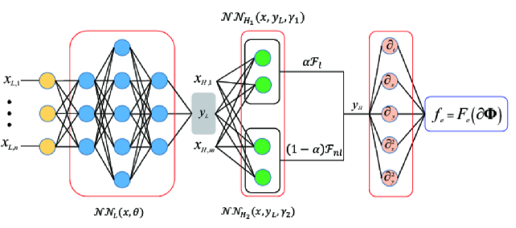
Figure 1: Schematic of the multi-fidelity DNN and MPINN. The left box (blue nodes) represents the low-fidelity DNN $\mathcal{NN}_{L}(x,\theta)$ connected to the box with green dots representing two high fidelity DNNs, $\mathcal{NN}_{H_{i}}(x,y_{L},\gamma_{i})$ ($i=1,2$). In the case of MPINN, the combined output of the two high-fidelity DNNs is input to an additional PDE-induced DNN. Here $\partial\bm{\Phi}=\left[\partial_{t},\partial_{x},\partial_{y},\partial^{2}_{x},\partial^{2}_{y},...\right]y_{H}$ denotes symbolically the last DNN that has a very complicated graph and its structure is determined by the specific PDE considered.

The architecture of the proposed multi-fidelity DNN and MPINN is illustrated in Fig. 1, which is composed of four fully-connected neural networks. The first one $\mathcal{NN}_{L}(x_{L},\theta)$ is employed to approximate the low-fidelity data, while the second and third NNs ($\mathcal{NN}_{H_{i}}(x,y_{L},\beta,\gamma_{i}),i=1,2$) are for approximating the correlation for the low- and high-fidelity data; the last NN ($\mathcal{NN}_{f_{e}}$) is induced by encoding the governing equations, e.g. the partial differential equations (PDEs). In addition, $\mathcal{F}_{l}=\mathcal{NN}_{H_{1}}$, and $\mathcal{F}_{nl}=\mathcal{NN}_{H_{2}}$; $\theta$, $\alpha$, $\beta$, and $\gamma_{i},i=1,2$ are unknown parameters of the NNs, which can be learned by minimizing the following loss function:

$$MSE=MSE_{y_{L}}+MSE_{y_{H}}+MSE_{f_{e}}+\lambda\sum\beta_{i}^{2},$$ (6)

where

$$MSE_{y_{L}} =\frac{1}{N_{y_{L}}}\sum^{N_{y_{L}}}_{i=1}\left(|y^{*}_{L}-y_{L}|^{2}+|\nabla y^{*}_{L}-\nabla y_{L}|^{2}\right),$$ (7)

$$MSE_{y_{H}} =\frac{1}{N_{y_{H}}}\sum^{N_{y_{H}}}_{i=1}\left(|y^{*}_{H}-y_{H}|^{2}\right),$$ (8)

$$MSE_{f_{e}} =\frac{1}{N_{f}}\sum^{N_{f}}_{i=1}\left(|f^{*}_{e}-f_{e}|^{2}\right).$$ (9)

Here, $\psi$ ($\psi=y^{*}_{L},\leavevmode\nobreak\ y^{*}_{H}$, and $f^{*}_{e}$) denote the outputs of the $\mathcal{NN}_{L}$, $\mathcal{NN}_{H}$, and $\mathcal{NN}_{f_{e}}$, $\beta$ is any weight in $\mathcal{NN}_{L}$ and $\mathcal{NN}_{H_{2}}$ as well as $\alpha$, and $\lambda$ is the $L_{2}$ regularization rate. It is worth mentioning that the boundary/initial conditions for $f_{e}$ can also be added into the loss function, in a similar fashion as in the standard PINNs introduced in detail in [22] so we do not elaborate on this issue here. In the present study, the loss function is optimized using the L-BFGS method together with Xavier’s initialization method, while the hyperbolic tangent function is employed as the activation function in $\mathcal{NN}_{L}$ and $\mathcal{NN}_{H_{2}}$. We note that no activation function is included in $\mathcal{NN}_{H_{1}}$ due to the fact that it is used to approximate the linear part of $\mathcal{F}$. Hence, the present DNNs can dynamically learn the linear as well as the nonlinear correlations without any prior knowledge on the correlation for the low- and high-fidelity data.

3 Results and Discussion

Next we present several tests of the multi-fidelity DNN as well as the MPINN, the latter in the context of two inverse PDE problems related to geophysical applications.

3.1 Function approximation

We first demonstrate the effectiveness of this multi-fidelity modeling in approximating both continuous and discontinuous functions based on both linear and complicated nonlinear correlations between the low- and high-fidelity data.

3.1.1 Continuous function with linear correlation

We first consider a pedagogical example of approximating an one-dimensional function based on data from two levels of fidelities. The low- and high-fidelity data are generated from:

$$y_{L}(x) =A(6x-2)^{2}\sin(12x-4)+B(x-0.5)+C,\leavevmode\nobreak\ \leavevmode\nobreak\ x\in[0,1]$$ (10)

$$y_{H}(x) =(6x-2)^{2}\sin(12x-4),$$ (11)

where $y_{H}$ is linear with $y_{L}$, and A = 0.5, B = 10, C = -5. As shown in Fig. 2, the training data at the low- and high-fidelity level are $x_{L}=\{0,0.1,0.2,0.3,0.4,0.5,0.6,\\ 0.7,0.8,0.9,1\}$ and $x_{H}=\{0,0.4,0.6,1\}$, respectively.

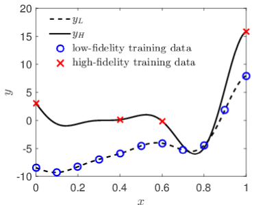
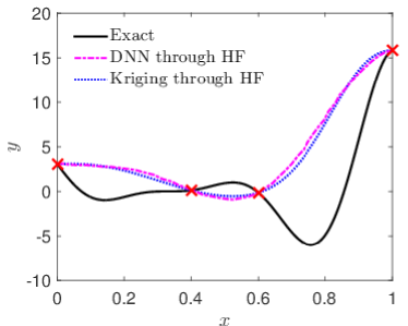
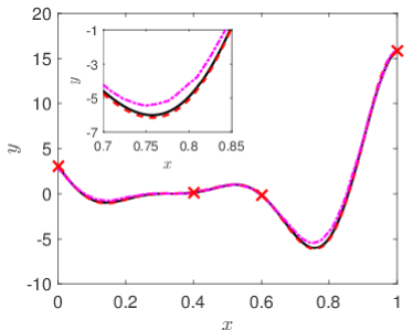
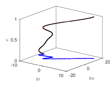
Figure 2: Approximation of a continuous function from multi-fidelity data with linear correlation. (a) Training data at low- (11 data points) and high-fidelity levels (4 data points). (b) Predictions from DNN using high-fidelity data only; also included are the results of Kriging. (c) Predictions from the multi-fidelity DNN (Red dashed line) and Co-Kriging [6]) (Magenta dotted line). (d) The Red dashed line in the $(x,y_{L},y_{H})$ plane represents Eq. (3) (on top of the exact Black solid line) and the Red dashed line in the $(y_{L},y_{H})$ plane represents the correlation discovered between the high- and low-fidelity data; the Blue solid line is the exact correlation.

We first try to predict the true function using the high-fidelity data only. For this case, we only need to keep $\mathcal{NN}_{H_{2}}$ (Fig. 1). In addition, the input for $\mathcal{NN}_{H_{2}}$ becomes $x$ because no low-fidelity data are available. Here 4 hidden layers and 20 neurons per layer are adopted in $\mathcal{NN}_{H_{2}}$ and no regularization is used. The learning rate is set as 0.001. As we can see in Fig. 2, the present model provides inaccurate predictions due to the lack of sufficient high-fidelity data. Furthermore, we also plot the predictive posterior means of the Kriging [6], which is noted to be similar as the results from the $\mathcal{NN}_{H_{2}}$. Keeping the high-fidelity data fixed, we try to improve the accuracy of prediction by adding low-fidelity data (Fig. 2). In this case, the last DNN for the PDE is discarded. Here 2 hidden layers and 20 neurons per layer are used in $\mathcal{NN}_{L}$, while 2 hidden layers with 10 neurons per layer are employed for $\mathcal{NN}_{H_{2}}$, and only 1 hidden with 10 neurons are used in $\mathcal{NN}_{H_{1}}$ (The size of $\mathcal{NN}_{H_{1}}$ is kept identical in all of the following cases). The regularization rate is set to $\lambda=10^{-2}$ with a learning rate 0.001. As shown in Fig. 2, the present model provides accurate predictions for the high-fidelity profile. In addition, the prediction using the Co-Kriging is displayed in Fig. 2 [6]. We see that the learned profiles from these two methods are similar, while the result from the present model is slightly better than the Co-Kriging, which can be seen in the inset of Fig. 2. Finally, the estimated correlation is illustrated in Fig. 2, which also agrees quite well with the exact result. Unlike the Co-Kriging/GPR, no prior knowledge on the correlation between the low- and high-fidelity data is needed in the multi-fidelity DNN, indicating that the present model can learn the correlation dynamically based on the given data.

The size of the neural network (e.g., depth and width) has a strong effect on the predictive accuracy [22], which is also investigated here. Since we have sufficient low-fidelity data, it is easy to find an appropriate size for $\mathcal{NN}_{L}$ to approximate the low-fidelity function. Therefore, the particular focus is put on the size of $\mathcal{NN}_{H_{2}}$ due to the fact that the few high-fidelity data may yield overfitting. Note that since the correlation between the low- and high-fidelity data is relatively simple, there is no need to set the $\mathcal{NN}_{H_{2}}$ to have a large size. Hence, we limit the ranges of the depth (i.e., $l$) and width (i.e., $w$) as: $l\in[1,4]$ and $w\in[2,32]$, respectively. Considering that a random initialization is utilized, we perform ten runs for each case with different depth and width. The mean and standard deviation for the relative $L_{2}$ errors defined as

$$E=\frac{1}{N}\sum^{n=N}_{n=1}\sqrt{\frac{\sum_{j}(y^{*}_{j}-y_{j})^{2}}{\sum y^{2}_{j}}},\leavevmode\nobreak\ \sigma=\sqrt{\frac{\sum^{n=N}_{n=1}(E_{n}-E)^{2}}{N}},$$ (12)

are used to quantify the effect of the size of the $\mathcal{NN}_{H_{2}}$. In Eq. (12), $E$ is the mean relative $L_{2}$ errors, $n$ is the index of each run, $N$ is the total number of runs ($N=10$), $j$ is the index for each sample data points, $E_{n}$ is the relative $L_{2}$ error for the $n-th$ run, and the definitions of $y^{*}$ and $y$ are the same as those in Sec. 1. As shown in Table 1, the computational errors for $\mathcal{NN}_{H_{2}}$ with different depth and width are almost the same. In addition, the standard deviation for the relative $L_{2}$ errors are not presented because they are less than $10^{-5}$ for each case. All these results demonstrate the robustness of the multi-fidelity DNNs. To reduce the computational cost as well and retain the accuracy, a good choice for the size of $\mathcal{NN}_{H_{2}}$ may be $l\in[1,2]$ and $w\in[4,20]$ in low dimensions.

Table 1: Mean relative $L_{2}(\times 10^{-3})$ for NNs with different sizes.

	4	8	16	32
1	3.1	3.0	4.6	2.9
2	3.4	3.0	3.0	3.1
3	3.1	3.1	3.1	3.0
4	3.0	3.0	3.0	3.0

3.1.2 Discontinuous function with linear correlation

As mentioned in [7], the approximation of a discontinuous function using GPR is challenging due to the continuous kernel employed. We then proceed to test the capability of the present model for approximating discontinuous functions. The low- and high-fidelity data are generated by the following “Forrester” functions with jump [7]:

$$y_{L}(x)=\left\{\begin{aligned} &0.5(6x-2)^{2}\sin(12x-4)+10(x-0.5)-5,\leavevmode\nobreak\ 0\leq x\leq 0.5,\\ &3+0.5(6x-2)^{2}\sin(12x-4)+10(x-0.5)-5,\leavevmode\nobreak\ 0.5<x\leq 1,\end{aligned}\right.$$ (13)

and

$$y_{H}(x)=\left\{\begin{aligned} &2y_{L}(x)-20x+20,\leavevmode\nobreak\ 0\leq x\leq 0.5,\\ &4+2y_{L}(x)-20x+20,\leavevmode\nobreak\ 0.5<x\leq 1.\end{aligned}\right.$$ (14)

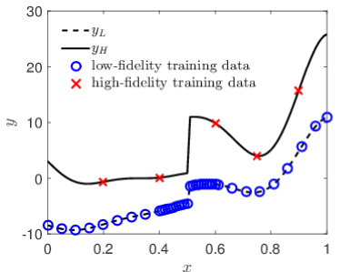
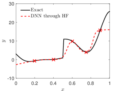
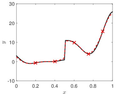
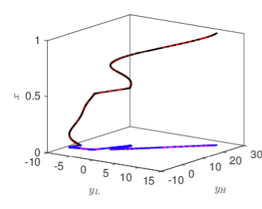
Figure 3: Approximation of a discontinuous function from multi-fidelity data with linear correlation. (a) Training data at low- (38 data points) and high-fidelity levels (5 data points). (b) Predictions from DNN using high-fidelity data only (Red dash line); also included is the exact curve (Black solid line). (c) Predictions from multi-fidelity DNN for high-fidelity (Red dash line). (d) The Red dashed line in the $(x,y_{L},y_{H})$ plane represents Eq. (3) (on top of the exact Black solid line) and the Red dashed line in the $(y_{L},y_{H})$ plane represents the correlation discovered between the high- and low-fidelity data; the Blue line is the exact correlation.

As illustrated in Fig. 3, 38 and 5 sampling data points are employed as the training data at the low- and high-fidelity level, respectively. The learning rate is again set as 0.001 for all test cases here. Similarly, we employ the $\mathcal{NN}_{H_{2}}$ ($l\times w=4\times 20$) to predict the high-fidelity values on the basis of the given high-fidelity data only, but the corresponding prediction is not good (Fig. 3). However, using the multi-fidelity data, the present model can provide quite accurate predictions for the high-fidelity profile (Fig. 3). Remarkably, the multi-fidelity DNN can capture the discontinuity at $x=0.5$ at the high-fidelity level quite well even though no data are available in the range $0.4<x<0.6$. This is reasonable because the low- and high-fidelity data share the same trend as $0.4<x<0.6$, yielding the correct predictions of the high-fidelity values in this zone. Furthermore, the learned correlation is displayed in Fig. 3, which shows only slight differences from the exact correlation.

3.1.3 Continuous function with nonlinear correlation

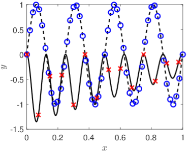
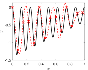
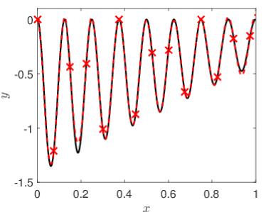
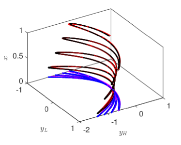
Figure 4: Approximation of a continuous function from multi-fidelity data with nonlinear correlation. (a) Training data at low- (51 data points) and high-fidelity levels (14 data points). Black solid line: High-fidelity values, Black dashed line: Low-fidelity values, Red cross: High-fidelity training data, Blue circle: Low-fidelity training data. (b) Predictions from high-fidelity DNN (Red dashed line); Black solid line: Exact values. (c) Predictions from multi-fidelity DNN for high-fidelity (Red dash line). (d) The Red dashed line in $(x,y_{L},y_{H})$ represents Eq. (3) (on top of the exact Black solid line) and the Red dashed line in $(y_{L},y_{H})$ represents the correlation discovered between the high- and low-fidelity data; the Blue line is the exact correlation.

To test the present model for capturing complicated nonlinear correlations between the low- and high-fidelity data, we further consider the following case [9]:

$$y_{L}(x) =\sin(8\pi x),\leavevmode\nobreak\ x\in[0,1],$$ (15)

$$y_{H}(x) =(x-\sqrt{2})y^{2}_{L}(x).$$ (16)

Here, we employ 51 and 14 data points (uniformly distributed) for low- and high-fidelity, respectively, as the training data, (Fig. 4). The learning rate for all test cases is still 0.001. As before, the $\mathcal{NN}_{H_{2}}$ ($l\times w=4\times 20$) cannot provide accurate predictions for the high-fidelity values using only the few high-fidelity data points as displayed in Fig. 4. We then test the performance of the multi-fidelity DNN based on the multi-fidelity training data. Four hidden layers and 20 neurons per layer are used in $\mathcal{NN}_{L}$, and 2 hidden layers with 10 neurons per layer are utilized for $\mathcal{NN}_{H_{2}}$. Again, the predicted profile from the present model agrees well with the exact profile at the high-fidelity level, as shown in Fig. 4. It is interesting to find that the multi-fidelity DNN can still provide accurate predictions for the high-fidelity profile even though the trend for the low-fidelity data is opposite to that of the high-fidelity data, e.g., $0<x<0.2$, a case of adversarial type of data. In addition, the learned correlation between the low- and high-fidelity data agree well with the exact one as illustrated in Fig. 4, indicating that the multi-fidelity DNN is capable of discovering the non-trivial underlying correlation on the basis of training data.

3.1.4 Phase-shifted oscillations

For more complicated correlations between the low and high-fidelity data, we can easily extend the multi-fidelity DNN based on the “embedding theory” to enhance the capability for learning more complex correlations [25] (For more details on the embedding theory, refer to A). Here, we consider the following low-/high-fidelity functions with phase errors [25]:

$$y_{H}(x) =x^{2}+\sin^{2}(8\pi x+\pi/10),$$ (17)

$$y_{L}(x) =\sin(8\pi x).$$ (18)

We can further write $y_{H}$ in terms of $y_{L}$ as

$$y_{H}=x^{2}+(y_{L}\cos(\pi/10)+y^{(1)}_{L}\sin(\pi/10))^{2},$$ (19)

where $y^{(1)}_{L}$ denotes the first derivatives of $y_{L}$. The relation between the low- and high-fidelity data is displayed in Fig. 5, which is rather complicated. The performance of the multi-fidelity DNN for this case will be tested next. To approximate the high-fidelity function, we select 51 and 16 uniformly distributed sample points as the training data for low- and high-fidelity values, respectively (Fig. 5). The selected learning rate for all test cases is 0.001. Here, we test two types of inputs for $\mathcal{NN}_{H_{2}}$, i.e., $[x,y_{L}(x)]$ (Method I), and $[x,y_{L}(x),y_{L}(x-\tau)]$ (Method II) ($\tau$ is the delay). Four hidden layers and 20 neurons per layer are used in $\mathcal{NN}_{L}$, and 2 hidden layers with 10 neurons per layer are utilized for $\mathcal{NN}_{H_{2}}$. As shown in Fig. 5, it is interesting to find that Method II provides accurate predictions for the high-fidelity values (Fig. 5), while Method I fails (Fig. 5). As mentioned in [25], the term $y_{L}(x-\tau)$ can be viewed as an implicit approximation for $y^{(1)}_{L}$, which enables Method II to capture the correlation in Eq. (19) based only on a small number of high-fidelity data points. However, given that no information on $y^{(1)}_{L}$ is available in Method I, the present datasets are insufficient to obtain the correct correlation.

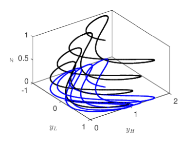
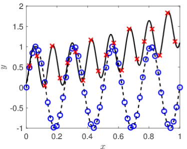
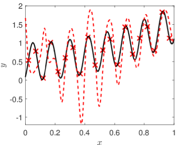
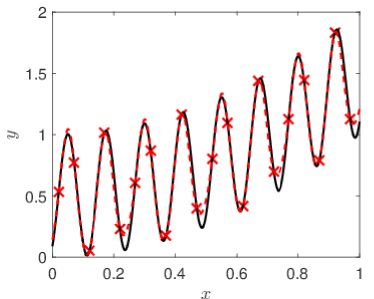
Figure 5: Approximation of continuous function from multi-fidelity data with phase-shifted oscillations and highly-nonlinear correlation: (a) Correlation among $x$, $y_{L}$, and $y_{H}$. The Blue line represents the projection in the $(y_{L},y_{H})$ plane. (b) Training data for $y_{L}$ and $y_{H}$. Black solid line: Exact high-fidelity values; Black dashed line: Exact low-fidelity values; Red cross: High-fidelity training data; Blue circle: Low-fidelity training data. (c) Predictions from Method I (without time-delay) (Red dashed line). (d) Predictions from Method II (with time-delay) (Red dashed line). The learned optimal value for $\tau$ is $4.49\times 10^{-2}$.

3.1.5 20-dimensional function approximation

In principle, the new multi-fidelity DNN can approximate any high-dimensional function so here we take a modest size so that is not computationally expensive to train the DNN. Specifically, we generate the low- and high-fidelity data for a 20-dimensional function from the following equations: [26]

$$y_{H}(x) =(x_{1}-1)^{2}+\sum^{20}_{i=2}\left(2x^{2}_{i}-x_{i-1}\right)^{2},x_{i}\in[-3,3],i=1,2,...,20,$$ (20)

$$y_{L}(x) =0.8y_{H}(x)-\sum^{19}_{i=1}0.4x_{i}x_{i+1}-50.$$ (21)

As shown in Fig. 6, using only the available high-fidelity data does not lead to an accurate function approximation but using the multi-fidelity DNN approach gives excellent results as shown in Fig. 6.

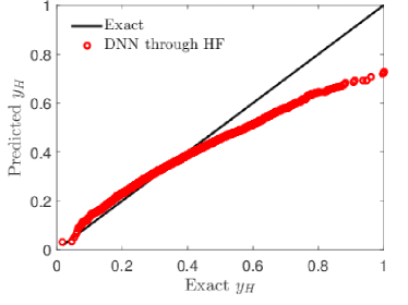
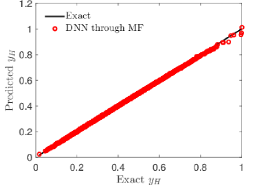
Figure 6: Approximations of the 20-dimensional function (learning rate: 0.001). (a) Single-fidelity predictions from high-fidelity data. $\mathcal{NN}_{H_{2}}\rightarrow 4\times 160$ with 5000 randomly selected high-fidelity data, and 10000 test data at random locations. (b) Multi-fidelity DNN predictions. $\mathcal{NN}_{L}\rightarrow 4\times 128$, $\mathcal{NN}_{H_{2}}\rightarrow 2\times 64$ with 30000 and 5000 randomly selected low-/high-fidelity data, and 10000 test data at random locations.

In summary, in this section we have demonstrated using different data sets and correlations that multi-fidelity DNNs can adaptively learn the underlying correlation between the low- and high-fidelity data from the given datasets without any prior assumption on the correlation. In addition, they can be applied to high-dimensional cases, hence outperforming GPR [9]. Finally, the present framework can be easily extended based on the embedding theory to non-functional correlations, which enables multi-fidelity DNNs to learn more complicated nonlinear correlations induced by phase errors of the low-fidelity data (adversarial data).

3.2 Inverse PDE problems with nonlinearities

In this section, we will apply the multi-fidelity PINNs (MPINNs) to two inverse PDE problems with nonlinearities, specifically, unsaturated flows and reactive transport in porous media. We assume that the hydraulic conductivity is first estimated based on scarce high-fidelity measurements of the pressure head. Subsequently, the reactive models are further learned given a small set of high-fidelity observations of the solute concentration.

3.2.1 Learning the hydraulic conductivity for nonlinear unsaturated flows

Unsaturated flows play an important role in the ground-subsurface water interaction zone [27, 28]. Here we consider a steady unsaturated flow in an one-dimensional (1D) column with a variable water content, which can be described by the following equation as

$$\partial_{x}\left(K(h)\partial_{x}h\right)=0.$$ (22)

We consider two types of boundary conditions, i.e., (1) constant flux at the inlet and constant pressure head at the outlet, $q=-K\partial_{x}h=q_{0},\leavevmode\nobreak\ x=0;\leavevmode\nobreak\ h=h_{1},\leavevmode\nobreak\ x=L_{x}$ (Case I), and (2) constant pressure head at both the inlet and outlet, $h=h_{0},\leavevmode\nobreak\ x=0;\leavevmode\nobreak\ h=h_{1},\leavevmode\nobreak\ x=L_{x}$ (Case II). Here $L_{x}=200cm$ is the length of the column, $h$ is the pressure head, $h_{0}$ and $h_{1}$ are, respectively, the pressure head at the inlet and outlet, $q$ represents the flux, and $q_{0}$ is the flux at the inlet, which is a constant. In addition, $K(h)$ denotes the pressure-dependent hydraulic conductivity, which is expressed as

$$K(h)=K_{s}S^{1/2}_{e}\left[1-(1-S^{1/m}_{e})^{m}\right]^{2},$$ (23)

where $K_{s}$ is the saturated hydraulic conductivity, and $S_{e}$ is the effective saturation that is a function of $h$. It is noted that several models have been developed to characterize $S_{e}$ but among them, the van Genuchten model is the most widely used [29], which reads as follows:

$$S_{e}=\frac{1}{(1+|\alpha_{0}h|^{n})^{m}},\leavevmode\nobreak\ m=1-1/n.$$ (24)

In Eq. (24), $\alpha_{0}$ is related to the inverse of the air entry suction, and $m$ represents a measure of the pore-size distribution. To obtain the velocity field for later applications, we should first obtain the distribution of $K(h)$. Unfortunately, both parameters depend on the geometry of porous medium and are difficult to measure directly. We note that the pressure head can be measured more easily in comparison to $\alpha_{0}$ and $m$. Therefore, we assume that partial measurements of $h$ are available without the direct measurements of $\alpha_{0}$ and $m$. The objective is to estimate $\alpha_{0}$ and $m$ based on the observations of $h$. Then, we can compute the distribution of $K(h)$ according to Eqs. (23) and (24).

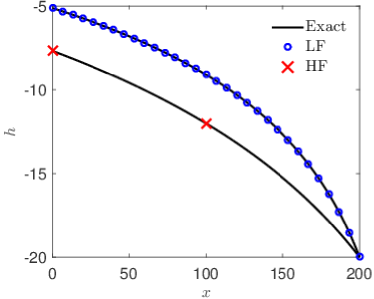
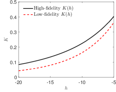
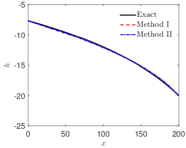
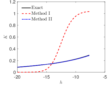
Figure 7: Predictions for unsaturated flow in porous media using the differential (Eq. (22)) and integral formulations (Eq. (26)) with constant flux at the inlet and constant pressure head at the outlet. (a) Training data for pressure head. (b) Low- and high-fidelity hydraulic conductivity. (c) Predicted pressure head using MPINNs training with multi-fidelity data. Method I: Differential formulation, Method II: Integral formulation. (d) Predicted hydraulic conductivity using MPINNs training with multi-fidelity data. Method I: Differential formulation, Method II: Integral formulation.

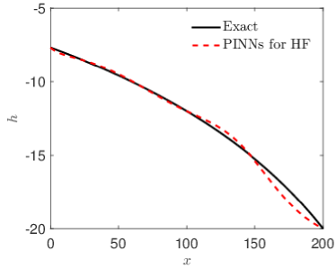
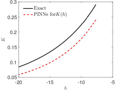
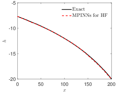
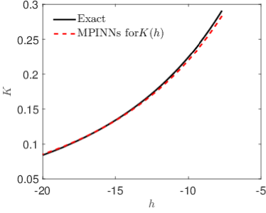
Figure 8: Predictions for unsaturated flow in porous media using the integral formulation (Eq. (26)) with constant flux at the inlet and constant pressure head at the outlet. (a) Predicted pressure head using PINNs training with high-fidelity data only. (b) Predicted hydraulic conductivity using PINNs training with high-fidelity data only. (c) Predicted pressure head using MPINNs with multi-fidelity data. (d) Predicted hydraulic conductivity using using MPINNs with multi-fidelity data.

The loam is selected as a representative case here, for which the empirical ranges of $\alpha_{0}$ and $m$ are: $\alpha_{0}(cm^{-1})\in[0.015,0.057]$ and $m\in[0.31,0.40]$ [30]. In addition, $K_{s}=1.04cm/hr$. To obtain the training data for neural networks, two types of numerical simulations are conducted to generate the low- and high-fidelity data using the bvp4c in Matlab (uniform lattice with $\delta_{x}=1/15cm$). For high-fidelity data, the exact values for $\alpha_{0}$ and $m$ are assumed to be 0.036 $cm^{-1}$ and 0.36. The high-fidelity simulations are then conducted using the exact values of $\alpha_{0}$ and $m$. Different initial guesses for $\alpha_{0}$ and $m$ are employed in the low-fidelity simulations. Specifically, ten uniformly distributed pairs i.e., $(\alpha_{0},m)$ in the range $(0.015,0.31)-(0.057,0.40)$ are adopted in the low-fidelity simulations. For all cases, 31 uniformly distributed sampling data at the low-fidelity level are served as the training data, and only two sampling points including the boundary conditions mentioned above are employed as the training data for high-fidelity. In addition, a smaller learning rate i.e., $10^{-4}$ is employed for all test cases in this section.

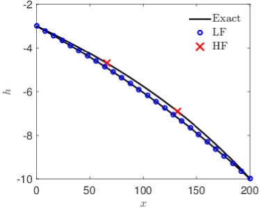
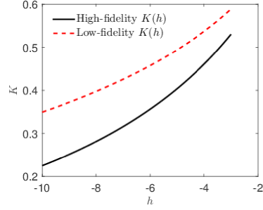
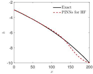
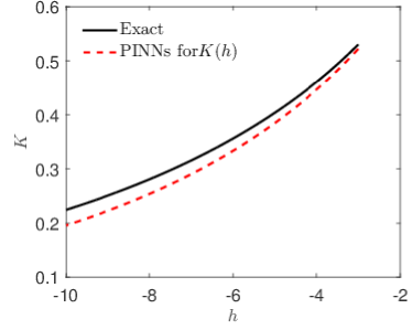
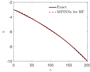
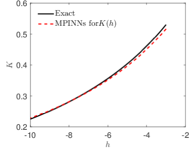
Figure 9: Predictions for unsaturated flow in porous media using the integral formulation (Eq. (26)) with constant pressure head at the inlet and outlet. (a) Training data for pressure head. Low-fidelity data is computed with $\alpha_{0}=0.015$ and $m=0.31$. (b) Low- and high-fidelity hydraulic conductivity. Low-fidelity hydraulic conductivity is computed with $\alpha_{0}=0.015$ and $m=0.31$. (c) Predicted pressure head using PINNs training with high-fidelity data only. (d) Predicted hydraulic conductivity using PINNs training with high-fidelity data only. (e) Predicted pressure head using MPINNs with multi-fidelity data. (f) Predicted hydraulic conductivity using using MPINNs with multi-fidelity data.

We first consider the flow with constant flux inlet. The flux at the inlet and the pressure at the outlet are set as $q_{0}=0.01cm/y$ and $h_{1}=-20cm$, respectively. Equation (22) is added into the last neural network in MPINNs. We employ the numerical results for $\alpha_{0}=0.055$ and $m=0.4$ as the low-fidelity data. As shown in Fig. 7, the prediction for hydraulic conductivity is different from the exact solution. According to Darcy’s law, we can rewrite Eq. (22) as

$$q(x)=-K\partial_{x}h,\leavevmode\nobreak\ \partial_{x}q(x)=0.$$ (25)

Considering that $q=q_{0}$ at the inlet is a constant, we can then obtain the following equation

$$q(x)=-K\partial_{x}h=q_{0},$$ (26)

which actually is the mass conservation at each cross section. We then employ Eq. (26) instead of Eq. (22) in the MPINNs, and the results improve greatly (Fig. 7).

We proceed to study this case in some more detail. We perform the single-fidelity modeling (SF) based on the high-fidelity data. We use two hidden layers with 20 neurons per layer in $\mathcal{NN}_{H_{2}}$, in which the hyperbolic tangent function is employed as the activation function. The learned pressure head and the hydraulic conductivity are shown in Figs. 8-8. We observe that both the learned $h$ and $K(h)$ disagree with the exact results. We then switch to multi-fidelity modeling. Two hidden layers and 10 neurons per layer are used in $\mathcal{NN}_{L}$, and two hidden layers with 10 neurons per layer are utilized for $\mathcal{NN}_{H_{2}}$. The predicted pressure head as well as the hydraulic conductivity (average value from ten runs with different initial guesses) agree quite well with the exact values (Figs. 8-8). For Case II, we set the pressure head at the inlet and outlet as $h_{0}=-3cm$ and $h_{1}=-10cm$. We also assume that the flux at the inlet is known, thus Eq. (26) can also be employed instead of Eq. (22) in the MPINNs. The training data are illustrated in Fig. 9. The size of the NNs here is kept the same as that used in Case I. We observe that results for the present case (Figs. 9-9) are quite similar with those in Case I.

Finally, the mean values of $\alpha_{0}$ as well as the $m$ for different initial guesses are shown in Table 2, which indicates that the MPINNs can significantly improve the prediction accuracy as compared to the estimations based on the high-fidelity only (SF in Table 2).

Table 2: PINN and MPINN predictions for hydraulic conductivity.

	$\alpha_{0}(cm^{-1})$	$\sigma(\alpha_{0})$	$m$	$\sigma(m)$
SF (Case I)	$0.0438$	-	$0.359$	-
MF (Case I)	$0.0344$	$0.0027$	0.347	0.0178
SF (Case II)	$0.0440$	-	$0.377$	-
MF (Case II)	$0.0337$	$7.91\times 10^{-4}$	0.349	0.0037
Exact	$0.036$	-	$0.36$	-

3.2.2 Estimation of reaction models for reactive transport

We further consider a single irreversible chemical reaction in a 1D soil column with a length of 5$m$, which is expressed as

$$a_{r}A\rightarrow B,$$ (27)

where $A$, and $B$ are different solute. The above reactive transport can be described by the following advection-dispersion-reaction equation as

$$\partial_{t}(\psi C_{i})+q\partial_{x}C_{i}=\psi D\partial^{2}_{x}C_{i}-\psi v_{i}k_{f,r}C_{A}^{a_{r}},(i=A,B),$$ (28)

where $C_{i}(mol/L)$ is the concentration of any solute, $q$ is the Darcy velocity, $\psi$ is the porosity, $D$ is the dispersion coefficient, $k_{f,r}$ denotes the chemical reaction rate, $a_{r}$ is the order of the chemical reaction, both of which are difficult to measure directly, and $v_{i}$ is the stoichiometric coefficient with $v_{A}=a_{r}$, and $v_{B}=-1$. Here, we assume that the following parameters are known: $\psi=0.4$, $q=0.5m/y$, and $D=10^{-8}m/s^{2}$. The initial and boundary conditions imposed on the solute are expressed as

$$C_{A}(x,0)=C_{B}(x,0)=0,$$ (29)

$$C_{A}(0,t)=1,\leavevmode\nobreak\ C_{B}(0,t)=0,$$ (30)

$$\partial_{x}C_{i}(x,t)|_{x=l_{x}}=0.$$ (31)

The objective here is to learn the effective chemical reaction rate as well as the reaction order based on partial observations of the concentration field $C_{A}(x,t)$.

We perform lattice Boltzmann simulations [31, 32] to obtain the training data since we have no experimental data. Consider that $v_{A}$ is a constant, we define an effective reaction rate as $k_{f}=v_{A}k_{f,r}$ for simplicity. The exact effective reaction rate and reaction order are assumed to be $k_{f}=1.577/y$ and $a_{r}=2$, respectively. Numerical simulations with the exact $k_{f}$ and $a_{r}$ are then conducted to obtain the high-fidelity data. In simulations, a uniform lattice is employed, i.e., $l_{x}=400\delta_{x}$, where $\delta_{x}=0.0125m$ is the space step, and $\delta_{t}=6.67\times 10^{-4}y$ is the time step size. We assume that the sensors for concentration are located at $x=\{0.625,1.25,2.5,3.75\}m$. In addition, we assume that the data are collected from the sensors once half a year. In particular, we employ two different datasets (Fig. 10), i.e., (1) $t=0.5$ and 1 years (Case I), and (2) $t=0.25$ and 0.75 years. Schematics of the training data points for the two cases we consider are shown in Fig. 10 and Fig. 10.

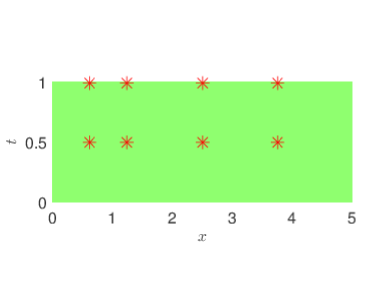
Figure 10: Schematic of the space-time domain and the locations of the high-fidelity data for modeling reactive transport. (a) Case I: Data are collected at $t=0.5$ and 1 years. (b) Case II: Data are collected at $t=0.25$ and 0.75 years.

Next, we describe how we obtain the low-fidelity data. In realistic applications, the pure chemical reaction rate (without porous media) between different solute e.g., $A$ and $B$ are known, which can be served as the initial guess for $k_{f}$. Here we assume that the initial guess for the chemical reaction rate and reaction order vary from $0.75k_{f}/a_{r}$ to $1.25k_{f}/a_{r}$. To study the effect of the initial guess ($(k_{f,0},a_{r0})$) on the predictions, we conduct the low-fidelity numerical simulations based on ten uniformly distributed pairs in $[0.75k_{f},0.75a_{r}]-[1.25k_{f},1.25a_{r}]$ using the same grid size and time step as the high-fidelity simulations. Here $k_{f,0}$ and $a_{r0}$ represent the initial guesses for $k_{f}$ and $a_{r}$. The learning rate employed in this section is also $10^{-4}$.

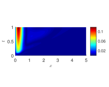
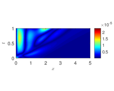
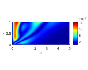
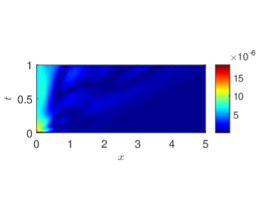
Figure 11: Predicted concentration field. (a) Case I: Relative errors (absolute value) using a PINN trained on high-fidelity data only. $\mathcal{NN}_{H_{2}}\rightarrow 4\times 20$. (b) Case I: Mean relative errors (absolute value) using a MPINN trained on multi-fidelity data. Initial guesses: ten uniformly distributed pairs in $[0.75k_{f},0.75a]-[1.25k_{f},1.25a]$. The concentration fields plotted are the mean values for ten runs with different initial guesses. $\mathcal{NN}_{L}\rightarrow 2\times 10$, $\mathcal{NN}_{H_{2}}\rightarrow 2\times 10$. (c) Case II: Relative errors (absolute value) using a PINN trained on high-fidelity data only. $\mathcal{NN}_{H_{2}}\rightarrow 4\times 20$. (d) Case II: Mean relative errors (absolute value) using a MPINN trained on multi-fidelity data. $\mathcal{NN}_{L}\rightarrow 2\times 10$, $\mathcal{NN}_{H_{2}}\rightarrow 2\times 10$.

The results of predictions using PINNs (with the hyperbolic tangent activation function) trained on high-fidelity data are shown in Fig. 11 and Fig. 11 for the two cases we consider, and corresponding results using MPINNs are shown in Fig. 11 and Fig. 11. The estimated mean and standard deviation for $k_{f}$ and $a_{r}$ are displayed in Table 3, which are much better than the results from single-fidelity modelings. We also note that the standard deviations are rather small, which demonstrates the robustness of the MPINNs.

Table 3: PINN and MPINN predictions for reactive transport.

	$k_{f}(/y)$	$\sigma(k_{f})$	$a_{r}$	$\sigma(a_{r})$
SF (Case I)	0.441	-	0.558	-
MF (Case I)	1.414	$7.45\times 10^{-3}$	1.790	$9.44\times 10^{-3}$
SF (Case II)	1.224	-	1.516	-
MF (Case II)	1.557	$2.14\times 10^{-2}$	1.960	$2.57\times 10^{-2}$
Exact	1.577	-	2	-

4 Conclusion

In this work we presented a new composite deep neural network that learns from multi-fidelity data, i.e. a small set of high-fidelity data and a larger set of inexpensive low-fidelity data. This scenario is prevalent in many cases for modeling physical and biological systems and we expect that the new DNN will provide solutions to many current bottlenecks where availability of large data sets of high-fidelity is simply not possible but either low-fidelity data from inexpensive sensors or other modalities or even simulated data can be readily obtained. Moreover, we extended the concept of physics-informed neural networks (PINNs) that use a single-fidelity data to train to the multi-fidelity case and MPINNs. Specifically, MPINNs are composed of four fully connected neural networks: the fist neural network approximates the low-fidelity data, while the second and third NNs are for constructing the correlations between the low- and high-fidelity data, and the last NN encodes the PDEs that describe the corresponding physical problems. The two sub-networks included in the high-fidelity network are employed to approximate the linear and nonlinear parts of the correlations, respectively. Training the relaxation parameter employed to combine the two sub-networks enables the MPINNs to learn the correlation based on the training data without any prior assumption on the relation between the low- and high-fidelity data.

MPINNs have the following attractive features: (1) Owing to the expressible capability of function approximation of the NNs, multi-fidelity NNs are able to approximate both continuous and discontinuous functions in high dimensions; (2) Due to the fact that NNs can handle almost any kind of nonlinearities, MPINNs are effective for identification of unknown parameters or functions in inverse problems described by nonlinear PDEs.

We first tested the new multi-fidelity DNN in approximating continuous and discontinuous functions with linear and nonlinear correlations. Our results demonstrated that the present model can adaptively learn the correlations between the low- and high-fidelity data based on the training data of variable fidelity. In addition, this model can easily be extended based on the embedding theory to learn more complicated nonlinear and non-functional correlations. We then tested MPINNs on inverse PDE problems, namely, in estimating the hydraulic conductivity for unsaturated flows as well as the reaction models in reactive transport in porous media. We found that the proposed new MPINN can identify the unknown parameters or even functions with high accuracy using very few high-fidelity data, which is promising in reducing the high experimental cost for collecting high-fidelity data. Finally, we point out that MPINNs can also be employed for high-dimensional problems as well as problems with multiple fidelities, i.e. more than two fidelities.

Appendix A Data-driven manifold embeddings

To learn more complicated non-linear correlation between the low- and high-fidelity data, we can further link the multi-fidelity DNNs with the embedding theory [25]. According to the weak Whitney embedding theorem [33], any continuous function from an $n$-dimensional manifold to an $m$-dimensional manifold may be approximated by a smooth embedding with $m>2n$. Using this theorem, Taken’s theorem [34] further points out that the $m$ embedding dimensions can be composed of $m$ different observations of the system state variables or $m$ time delays for a single scalar observable.

Now we will introduce the applications of the two theorems in multi-fidelity modelings. We assume that both $y_{L}$ and $y_{H}$ are smooth functions. Suppose that $y_{L},y_{L}(x-\tau),...,y_{L}(x-(m-1)\tau)$ ($\tau$ is the time delay) and a small number of $(x,y_{H})$ are available, we can then express $y_{H}$ in the following form

$$y_{H}(x)=\mathcal{F}(x,y_{L}(x),y_{L}(x-i\tau)),i=1,...,m-1.$$ (32)

By using this formulation, we can construct more complicate correlation than Eq. (2). To link the multi-fidelity DNN with the embedding theory, we can extend the inputs for $\mathcal{NN}_{H,i}$ to higher dimensions, i.e., $\left[x,y_{L}(x)\right]\rightarrow[x,y_{L}(x),y_{L}(x-\tau),y_{L}(x-2\tau),...,$ $y_{L}(x-(m-1)\tau)]$, which enables the multi-fidelity DNN to discover more complicated underlying correlations between the low- and high-fidelity data.

Note that the selection of optimal value for the time delay $\tau$ is important in embedding theory [35, 36, 37], on which numerous studies have been carried out [35]. However, most of the existing methods for determining the optimal value of $\tau$ appear to be problem-dependent [35]. Recently, Dhir et al. proposed a Bayesian delay embedding method, where $\tau$ is robustly learned from the training data by employing the variational autoencoder [37]. In the present study, the value of $\tau$ is also learned by optimizing the NNs rather than setting it as constant as in the original work presented in Ref. [25].

References

- [1] N. M. Alexandrov, R. M. Lewis, C. R. Gumbert, L. L. Green, P. A. Newman, Approximation and model management in aerodynamic optimization with variable-fidelity models, J. Aircraft 38 (6) (2001) 1093–1101.
- [2] D. Böhnke, B. Nagel, V. Gollnick, An approach to multi-fidelity in conceptual aircraft design in distributed design environments, in: 2011 Aerospace Conference, IEEE, 2011, pp. 1–10.
- [3] L. Zheng, T. L. Hedrick, R. Mittal, A multi-fidelity modelling approach for evaluation and optimization of wing stroke aerodynamics in flapping flight, J. Fluid Mech. 721 (2013) 118–154.
- [4] N. V. Nguyen, S. M. Choi, W. S. Kim, J. W. Lee, S. Kim, D. Neufeld, Y. H. Byun, Multidisciplinary unmanned combat air vehicle system design using multi-fidelity model, Aerosp. Sci. and Technol. 26 (1) (2013) 200–210.
- [5] M. C. Kennedy, A. O’Hagan, Predicting the output from a complex computer code when fast approximations are available, Biometrika 87 (1) (2000) 1–13.
- [6] A. I. Forrester, A. Sóbester, A. J. Keane, Multi-fidelity optimization via surrogate modelling, Proc. Math. Phys. Eng. Sci. 463 (2088) (2007) 3251–3269.
- [7] M. Raissi, G. E. Karniadakis, Deep multi-fidelity Gaussian processes, arXiv preprint arXiv:1604.07484, 2016.
- [8] M. Raissi, P. Perdikaris, G. E. Karniadakis, Inferring solutions of differential equations using noisy multi-fidelity data, J. Comput. Phys. 335 (2017) 736–746.
- [9] P. Perdikaris, M. Raissi, A. Damianou, N. Lawrence, G. E. Karniadakis, Nonlinear information fusion algorithms for data-efficient multi-fidelity modelling, Proc. Math. Phys. Eng. Sci. 473 (2198) (2017) 20160751.
- [10] L. Bonfiglio, P. Perdikaris, G. Vernengo, J. S. de Medeiros, G. E. Karniadakis, Improving swath seakeeping performance using multi-fidelity Gaussian process and Bayesian optimization, J. Ship Res. 62 (4) (2018) 223–240.
- [11] K. J. Chang, R. T. Haftka, G. L. Giles, I. J. Kao, Sensitivity-based scaling for approximating structural response, J. Aircraft 30 (2) (1993) 283–288.
- [12] R. Vitali, R. T. Haftka, B. V. Sankar, Multi-fidelity design of stiffened composite panel with a crack, Struct. and Multidiscip. O. 23 (5) (2002) 347–356.
- [13] M. Eldred, Recent advances in non-intrusive polynomial chaos and stochastic collocation methods for uncertainty analysis and design, in: 50th AIAA/ASME/ASCE/AHS/ASC Structures, Structural Dynamics, and Materials Conference 17th AIAA/ASME/AHS Adaptive Structures Conference 11th AIAA No, 2009, p. 2274.
- [14] A. S. Padron, J. J. Alonso, M. S. Eldred, Multi-fidelity methods in aerodynamic robust optimization, in: 18th AIAA Non-Deterministic Approaches Conference, 2016, p. 0680.
- [15] J. Laurenceau, P. Sagaut, Building efficient response surfaces of aerodynamic functions with Kriging and Cokriging, AIAA J. 46 (2) (2008) 498–507.
- [16] E. Minisci, M. Vasile, Robust design of a reentry unmanned space vehicle by multi-fidelity evolution control, AIAA J. 51 (6) (2013) 1284–1295.
- [17] P. Lancaster, K. Salkauskas, Surfaces generated by moving least squares methods, Math. Comput. 37 (155) (1981) 141–158.
- [18] D. Levin, The approximation power of moving least-squares, Math. Comp. 67 (224) (1998) 1517–1531.
- [19] M. G. Fernández-Godino, C. Park, N. H. Kim, R. T. Haftka, Review of multi-fidelity models, arXiv preprint arXiv:1609.07196, 2016.
- [20] H. Babaee, P. Perdikaris, C. Chryssostomidis, G. E. Karniadakis, Multi-fidelity modelling of mixed convection based on experimental correlations and numerical simulations, J. Fluid Mech. 809 (2016) 895–917.
- [21] Q. Zheng, J. Zhang, W. Xu, L. Wu, L. Zeng, Adaptive multi-fidelity data assimilation for nonlinear subsurface flow problems, Water Resour. Res. 55 (2018) 203–217.
- [22] M. Raissi, P. Perdikaris, G. E. Karniadakis, Physics-informed neural networks: A deep learning framework for solving forward and inverse problems involving nonlinear partial differential equations, J. Comput. Phys. 378 (2019) 686–707.
- [23] M. Raissi, A. Yazdani, G. E. Karniadakis, Hidden fluid mechanics: A Navier-Stokes informed deep learning framework for assimilating flow visualization data, arXiv preprint arXiv:1808.04327, 2018.
- [24] A. M. Tartakovsky, C. O. Marrero, D. Tartakovsky, D. Barajas-Solano, Learning parameters and constitutive relationships with physics informed deep neural networks, arXiv preprint arXiv:1808.03398, 2018.
- [25] S. Lee, F. Dietrich, G. E. Karniadakis, I. G. Kevrekidis, Linking Gaussian process regression with data-driven manifold embeddings for nonlinear data fusion, arXiv preprint arXiv:1812.06467, 2018.
- [26] S. Shan, G. G. Wang, Metamodeling for high dimensional simulation-based design problems, J. Mech. Design 132 (5) (2010) 051009.
- [27] S. L. Markstrom, R. G. Niswonger, R. S. Regan, D. E. Prudic, P. M. Barlow, Gsflow-coupled ground-water and surface-water flow model based on the integration of the precipitation-runoff modeling system (prms) and the modular ground-water flow model (modflow-2005), US Geological Survey techniques and methods 6 (2008) 240.
- [28] M. Hayashi, D. O. Rosenberry, Effects of ground water exchange on the hydrology and ecology of surface water, Groundwater 40 (3) (2002) 309–316.
- [29] M. T. Van Genuchten, A closed-form equation for predicting the hydraulic conductivity of unsaturated soils, Soil Sci. Soc. Am. J. 44 (5) (1980) 892–898.
- [30] R. F. Carsel, R. S. Parrish, Developing joint probability distributions of soil water retention characteristics, Water Resour. Res. 24 (5) (1988) 755–769.
- [31] X. Meng, Z. Guo, Localized lattice Boltzmann equation model for simulating miscible viscous displacement in porous media, J. Heat Mass Trans. 100 (2016) 767–778.
- [32] B. Shi, Z. Guo, Lattice Boltzmann model for nonlinear convection-diffusion equations, Phys. Rev. E 79 (1) (2009) 016701.
- [33] H. Whitney, Differentiable manifolds, Ann. Math. (1936) 645–680.
- [34] F. Takens, Detecting strange attractors in turbulence, in: Dynamical systems and turbulence, Warwick 1980, Springer, 1981, pp. 366–381.
- [35] R. Hegger, H. Kantz, T. Schreiber, Practical implementation of nonlinear time series methods: The tisean package, Chaos 9 (2) (1999) 413–435.
- [36] H. D. Abarbanel, R. Brown, J. J. Sidorowich, L. S. Tsimring, The analysis of observed chaotic data in physical systems, Rev. Mod. Phys. 65 (4) (1993) 1331.
- [37] N. Dhir, A. R. Kosiorek, I. Posner, Bayesian delay embeddings for dynamical systems, Conference on Neural Information Processing Systems, 2017.