Saec: Similarity-Aware Embedding Compression
in Recommendation Systems

Abstract

Production recommendation systems rely on embedding methods to represent various features. An impeding challenge in practice is that the large embedding matrix incurs substantial memory footprint in serving as the number of features grows over time. We propose a similarity-aware embedding matrix compression method called Saec to address this challenge. Saec clusters similar features within a field to reduce the embedding matrix size. Saec also adopts a fast clustering optimization based on feature frequency to drastically improve clustering time. We implement and evaluate Saec on Numerous, the production distributed machine learning system in Tencent, with 10-day worth of feature data from QQ mobile browser. Testbed experiments show that Saec reduces the number of embedding vectors by two orders of magnitude, compresses the embedding size by $\sim$27x, and delivers the same AUC and log loss performance.

1 Introduction

Embedding methods have attracted much attention recently. They are used in applications that need to learn continuous representations from discrete features. Word embedding ^{18, 19} is widely used in natural language processing (NLP), and embedding vector is also adopted in knowledge graphs ⁵, social networks ⁷, and recommendation systems ^{16, 9}. One can use an embedding vector to represent a word in NLP or a feature in recommendation systems.

Although embedding methods show promising benefits, they pose serious challenges especially when used in recommendation systems. Particularly, the size of an embedding matrix grows linearly with the number of the symbols. In a recommendation system, the number of features (i.e. symbols) can be hundreds of billions, which suggests that the size of the embedding matrix can be up to hundreds of GBs ¹⁷. In order to provide efficient lookup performance, embedding matrix has to be maintained in the DRAM. Yet DRAM is expensive, especially the high-density modules ^{22, 11}, and its capacity is limited (typically 128GB). For example a 32GB DDR4-2400 server DRAM module costs about USD$300–$350 as of Feb 2019 ¹; having 128GB memory implies a per-server cost of over USD$1,200. Further, storing the embedding matrix on multiple servers and using distributed serving leads to more complicated issues like synchronization. Therefore it is crucial to minimize the memory footprint of embedding matrix for recommendation systems.

Model compression is widely used as an effective solution to reduce the number of parameters and the model size. Various methods have been proposed, such as parameter pruning ¹³, parameter sharing ^{12, 8, 23}, compact architecture ^{21, 6, 20}, parameter quantization ², and knowledge distillation ¹⁵. Recently model compression has also been studied for embedding matrix ^{6, 20}.

Unfortunately existing compression methods do not work well for recommendation systems. First, most methods focus on CNNs, particularly the fully-connected layers which account for most of the model parameters ¹². However, in an recommendation model, fully-connected layers only occupy a small fraction of the parameters ^{16, 9}. Second, compression methods for embedding matrix ^{6, 20} are designed for NLP problems. The differences between NLP and recommendation systems are notable. In NLP, the number of words for the embedding matrix is fixed, whereas the number of features for recommendation tasks in practice is growing constantly as new data become available. Figure 1 shows that the number of features grows from less than $10^{7}$ to over $10^{8}$ in a 10-day production feature data trace from Tencent. (see 3.1 for more details). Further, embedding vectors may have different lengths in recommendation systems instead of a uniform length in NLP. In the embedding matrix from the same production feature data trace, 88.95% vectors have a length of 9 and 11.05% have 17.

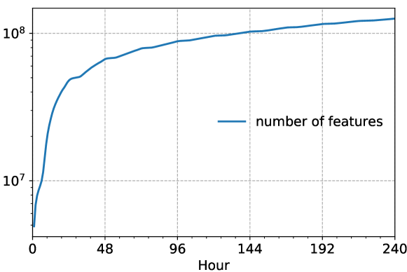
Figure 1: Time series of the number of features in a 10-day feature data trace from Tencent’s QQ mobile browser. Notice the log scale for the y-axis.

In this paper we propose to utilize two unique characteristics of recommendation systems, feature similarity and feature frequency, for embedding compression. First, embedding representations are usually over-parameterized: similar features have similar meanings and effects. We can use one embedding vector to express multiple similar features and in turn reduce the size of embedding matrix. Second, features appear in training data with different frequencies. Consequently the rare or less frequent features receive little training and have little impact or benefit to the overall performance ⁹. We can also compress these features with similar ones to reduce model size and improve their aggregated training effect.

We design an embedding compression framework called Saec to mine the similarity across features in recommendation systems. We make three new contributions.

• We propose a novel compression method based on $k$-means for embedding matrix in recommendation systems. Our method is field-aware: we apply $k$-means clustering on each field of features instead of on all features. A field contains a group of similar features with the same length generated by similar inputs in feature engineering. Field-aware clustering thus overcomes the challenge of non-uniform length of embedding vectors in recommendation systems.

• We design a fast clustering method to make Saec practical. As the feature data are enormous, clustering every single feature has formidable computation costs and is infeasible in practice where the model is trained say hourly. Since the feature frequency follows a heavy-tailed distribution, we cluster only a small fraction of the most frequent features and assign the other features to their closet centroids.

• We implement Saec in the production deep learning system in Tencent and evaluate it in a large-scale testbed with the production feature data trace from QQ mobile browser. Our evaluation shows that Saec (1) delivers the same AUC and log loss performance with $\sim$27x effective compression ratio taking into account its own overhead; and (2) accelerates clustering by 32x with fast clustering optimization.

We are optimizing our implementation of Saec and driving for the full deployment in Tencent.

2 Design

We now present Saec, our similarity-aware embedding compression framework based on $k$-means clustering.

2.1 Overview

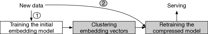
Figure 2: Training process in Saec. The gray steps are new in Saec.

Saec’s training process is shown in Figure 2. Like existing recommendation systems, Saec trains the embedding model continuously in a fixed time internal of say one hour with newly generated data. Each hour’s data are processed just once in one epoch instead of multiple epochs as used for other deep learning models in general. This initial model can be enormous. Saec then applies clustering to compress it into a much smaller model with only a subset of the original embedding vectors. Directly applying the compressed model generally results in poor prediction performance ¹². Thus Saec finally retrains the compressed model with the same data again in one epoch to compensate for the performance loss of compression.

As Saec does not change the training process for the initial model, we focus on its clustering method (2.2) and retraining strategy (2.3) in the following. We also discuss an optimization to accelerate clustering at the end (2.4).

2.2 Clustering Embedding Vectors

Our clustering method works on a field basis in order to overcome the variable embedding vector length problem as mentioned in 1. Our subsequent discussion assumes a particular field without loss of generality.

2.2.1 Field-Aware Clustering

Each field has its own embedding matrix $W\in\mathbb{R}^{n\times l}$ from the initial training, where $n$ is the number of features and $l$ the length of embedding vectors. In other words the embedding matrix is just a stack of embedding vectors, each representing a unique feature. Saec aims to cluster the original $n$ embedding vectors into just $k$ clusters, and for each cluster use one embedding vector to represent all the rest. Thus after compression there are $k$ representative embedding vectors which constitute the field’s codebook $C$. That is, $C=\left\{C_{1},C_{2},...,C_{k}\right\}$ where $C_{i}$ is an $l$-dimensional vector.

Now without clustering, we generally use a one-hot vector $X$ to encode a feature, and retrieve its corresponding embedding vector by a lookup with the embedding matrix $W$: $V=W^{T}X$ as shown in Figure 3. With clustering, to retrieve an embedding vector from the codebook, Saec in addition associates each feature with a mask. A table lookup transforms the feature’s one-hot vector to its mask which is an index that points to the corresponding representative embedding vector in the codebook. Figure 3 depicts the process. Generally $k\ll n$, and the codebooks and masks that Saec needs to store after clustering are also small.

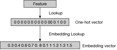
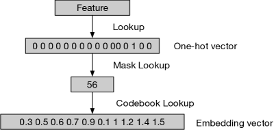
Figure 3: Embedding vector retrieval in Saec for (a) uncompressed features and (b) for compressed features.

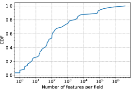
(a) CDF of per-field number of features

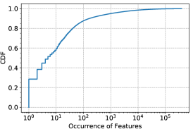
(b) CDF of feature frequency

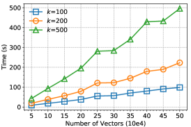
(c) Saec’s clustering time

Figure 4: Motivation figures for Saec’s design. For (a) and (b) the features are from one hour of 10-day feature data trace from Tencent QQ mobile browser. For (c) we show the time to run $k$-means clustering with different numbers of vectors using 1 CPU core of an Intel Xeon E5-2520 v3 at 2.4Ghz.

The central task is then to design an efficient clustering method that yields a good codebook. Mathematically, the problem can be posed as an optimization to find the best $k$ centroids, i.e. representative embedding vectors, that minimize the Euclidean distance between the original embedding vectors and the centroids:

$$\operatorname*{arg\,min}_{C}\displaystyle\sum_{i=1}^{k}\displaystyle\sum_{j=1}^{n}\|W_{j}-C_{i}\|^{2}.$$

This problem can then be solved by the well-known $k$-means clustering.

The number of features in a field is not uniform in practical recommendation system. For instance Figure 4(a) shows the distribution of per-field number of features in one hour of our 10-day feature data trace. We observe that only around 7% fields have more than $10^{5}$ features; most have less than $10^{4}$ features. It thus makes sense to focus on clustering the large fields to ensure the effectiveness of compression. We choose fields whose number of features is at least 100 times more than $k$ to go through the clustering process. As a reference $k$ is on the order of hundreds in our current design.

2.2.2 Centroid Initialization

Centroid initialization has a direct impact on the quality of clustering and thus the model performance. Here we examine three initialization methods, Random, $k$-means++, and Top-$k$ initialization which we propose.

Random. This method randomly chooses $k$ embedding vectors from the embedding matrix as the initial centroids. It does not consider the feature distribution or the parameter in the embedding vectors.

$k$-means++. This method chooses the first initial centroid uniformly at random. After that, each subsequent centroid is chosen according to a weighted probability based on the Euclidean distance between the potential candidate and the existing centroids ³. It aims to reduce the probability of having similar centroids.

Top-$k$. We propose this method to explore the feature frequency characteristics of recommendation systems. Figure 4(b) plots the CDF of feature frequency in our feature data trace. There is a clear heavy-tailed pattern: a very small number of frequent features appear much more often in the training data and receive much better training. Top-$k$ simply chooses $k$ most frequent embedding vectors as the initial centroids.

We conduct experiments in 3.3 to compare the prediction performance of these methods. The results show that Top-$k$ and $k$-means++ are both viable choices and $k$-means++ has the best accuracy performance. We thus choose $k$-means++ as the initialization method in the design.

2.3 Retraining to Optimize Codebooks

Model compression inherently leads to loss in inference accuracy which has been reported for parameter pruning, parameter sharing, etc ^{12, 13}. Retraining the compressed model is a common method to compensate the performance loss ¹⁴.

Saec also retrains the representative embedding vectors after clustering as the final step. Different from the initial training, in retraining the embedding vectors have to be retrieved and updated indirectly in both the forward pass and backpropagation. In the forward pass, Saec uses a feature’s mask to retrieve its corresponding representative embedding vector and then execute the forward process. The rest of computation is the same as the initial training. In backpropagation, each feature gets its own gradient. Saec then collects the gradients from features in the same cluster according to their mask and average them as the gradient of the representative embedding vector for updates. In other words, the representative vectors receive more extensive training now.

2.4 Fast Clustering

We have introduced Saec’s clustering method so far. An issue of our design is that clustering entails excessive computation cost: for production-scale systems, processing billions of embedding vectors may take well over an hour which is the typical training interval for recommendation models in practice. Figure 4(c) shows that running vanilla $k$-means over 50,000 vectors on a single thread with an Intel Xeon CPU already takes about 500s with $k=500$.

To make Saec more practical, we introduce a fast clustering optimization. We only process a part (100$k$ in our design) of the most frequent features and their embedding vectors in each field for clustering. The other embedding vectors are simply assigned with the nearest cluster centroids as their representative embedding vectors.

The rationale behind this design is that the clustering time grows proportionally with the number of vectors processed; Figure 4(c) clearly shows this trend when we run vanilla $k$-means. Yet as we showed in Figure 4(b), many features appear with low frequency. Prior work ⁹ shows that low frequency features cannot be trained well and do not have much benefit to the model performance. Reducing the number of features for clustering can therefore reduce the overhead dramatically without degrading performance.

3 Evaluation

We present our evaluation results in this section.

3.1 Setup

Prototype. We implement Saec on Numerous, a distributed machine learning system based on parameter server in Tencent. Our prototype consists of $\sim$1k LoC in C++ and follows our design in 2 including the fast clustering optimization. For load balance features are assigned to server nodes via hashing.

Testbed. We use a container based CPU testbed. Throughout the experiments the embedding models are trained with 50 worker containers and 40 server containers. Each worker has 6 vCPUs and 15GB memory; each server container has 2 vCPUs and 12.8GB memory.

Model and Datasets. We use Tencent’s recommendation model and the embedding matrix that serve the QQ mobile browser. The model is a modified DSSM ¹⁰. Different from the original DSSM, we directly adopt the embedding method to train the embedding matrix from scratch instead of using word2vec. Our model contains the embedding matrix and multiple fully-connected layers. The size of fully-connected layers is also different from the original DSSM. Saec does not change these fully-connected layers.

We collect a 10-day feature data trace from the QQ mobile browser, including features about users, user activities (search query tokens, watch times, etc.), news items, etc. as the training dataset. The feature data trace, with tens of TB of data, is collected on a hourly basis and has 240 segments each used for one epoch of training, following the same strategy of training in production.

We compare Saec against Baseline which is the original model with uncompressed embedding matrix. Both Baseline and Saec training use the same hyper-parameters: we adopt Adagrad as the optimizer and use a learning rate of 0.001.

Performance Metrics. Recommendation systems are commonly evaluated using AUC and log loss.

• AUC, area under the receiver operating curve, reflects the probability that a uniformly drawn positive item is ranked higher than a negative item by the model. It is the most widely used performance metric for recommendation tasks. AUC is calculated by:

  $$AUC=\int\limits_{0}^{1}TPR(t)d_{FPR(t)}.$$

  Here $t$ is the threshold which decides the TPR (true positive rate) and FPR (false positive rate). AUC is a value which ignores the distribution of samples. Generally, the higher the AUC is, the better the model is.

• Log loss is a natural measure of how close the predicted click probability is to the true 0-1 label in a statistical view ⁴. For binary classification tasks such as ours, the log loss is defined as:

  $$-\frac{1}{n}\sum_{i=1}^{n}y_{i}\log(p_{i})+(1-y_{i})\log(1-p_{i}),$$

  where $n$ is number of samples, $y_{i}$ is the true binary label of whether the user clicks the item for sample $i$, and $p_{i}$ is the click probability given by the model. The log loss value trends toward zero as the prediction becomes more accurate. If the distribution of positive and negative samples are uniform, the log loss is 0.693 for random prediction.

3.2 Overall Performance

Day	# vectors (Before)	# vectors (After)	AUC (Before)	AUC (After)	Log loss (Before)	Log loss (After)
1	$4.78\times 10^{7}$	$5.91\times 10^{5}$	0.737362	0.782574	0.402417	0.378207
2	$6.69\times 10^{7}$	$6.58\times 10^{5}$	0.780317	0.800837	0.375378	0.363054
3	$7.90\times 10^{7}$	$7.38\times 10^{5}$	0.798804	0.811197	0.358956	0.351107
4	$8.84\times 10^{7}$	$7.98\times 10^{5}$	0.805723	0.81675	0.356759	0.349559
5	$9.62\times 10^{7}$	$8.50\times 10^{5}$	0.80804	0.818024	0.355246	0.348736
6	$1.0\times 10^{8}$	$8.95\times 10^{5}$	0.811398	0.81524	0.354769	0.349977
7	$1.07\times 10^{8}$	$9.39\times 10^{5}$	0.815689	0.819183	0.345094	0.347014
8	$1.14\times 10^{8}$	$9.72\times 10^{5}$	0.814011	0.819918	0.352489	0.343376
9	$1.20\times 10^{8}$	$1.0\times 10^{6}$	0.816787	0.823498	0.308586	0.315366
10	$1.24\times 10^{8}$	$1.04\times 10^{6}$	0.817091	0.822134	0.347485	0.342201

Table 1: Performance results with the embedding matrix at the last hour of each day with the 10-day feature data trace.

We first evaluate the overall prediction performance of the model with Saec. The data segments as mentioned before are continuously fed to the model. We set $k$ to 100 so the condition to trigger compression for a field is it has at least $10^{4}$ features as explained in 2.2.1.

The embedding matrix keeps changing as the training proceeds with new feature data. Table 1 shows the performance results on a daily basis, where the ten models trained after the last hour of each day are used. We make several important observations.

First, as the number of embedding vectors in the original embedding matrix grows steadily with time, Saec consistently achieves significant compression by reducing two orders of magnitude for the number of embedding vectors. Note Saec also introduces overheads with masks as discussed in 2.2.1. Since $k$ is 100, we can encode the masks with 8 bits for each field. Now we can the obtain actual compression ratio of Saec, for say the final model after 240 epochs which is the last row in Table 1. Assume the length of vectors is 9 for simplicity. Then the size of the original embedding matrix is $1.24\times 10^{8}\times 36$ bytes, while the size after compression is $1.24\times 10^{8}\times 1+1.04\times 10^{6}\times 36$ bytes. That is, Saec achieves a compression ratio of 27.7.

Second, Saec’s compression does not degrade performance; in fact in most cases, the compressed model slightly outperforms the original one in both AUC and log loss as shown in Table 1. The final AUC of Saec is 82.22% which is 0.5% higher than Baseline; the final log loss of Saec is 0.342 while that of Baseline is 0.347. We believe there are two reasons for the performance improvement after compression. For one, the low frequency features may not receive enough training, as a result the original model has a good probability to give a wrong prediction with these poorly trained embedding vectors. After compression, more frequent embedding vectors are assigned to the low frequency features and then retrained, which improves the probability to make the right prediction. In addition, the input feature data have noise which may affect the accuracy of prediction. On the contrary, with Saec multiple features share the same embedding vector and more data are actually used to train these representative embedding vectors, which alleviates the influence of noise and leads to better prediction.

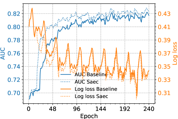
Figure 5: Model performance in Baseline and Saec during the complete training process.

Third, we also observe that while the AUC and log loss performance improves in general as time goes with more training, they sometimes deteriorate (e.g log loss in day 8 is worse than day 7). This performance oscillation is normal during training. To see this, we plot the time series of AUC and log loss of both Baseline and Saec for the 240-epoch training process in Figure 5. Clearly both performance metrics exhibit oscillation while they improve in general as training proceeds. The log loss performance shows more volatile oscillation than AUC. Nevertheless, Saec’s curves closely track those of Baseline.

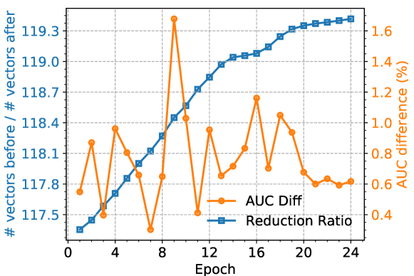
Figure 6: Saec’s reduction ratio in number of embedding vectors (# before / # after) and AUC improvement (AUC after $-$ AUC before) in the last 24 epochs.

Lastly, we zoom into Saec’s hourly performance within a day to better analyze it. We plot Saec’s reduction ratio in number of embedding vectors against its AUC improvement (AUC after $-$ AUC before) for the last 24 epochs of training in Figure 6. We observe that the reduction ratio steadily increases. This is because as the original embedding matrix gets larger more fields meet Saec’s clustering threshold and undergo compression. At the same time, the AUC of Saec is always better than Baseline which is consistent with the results presented before.

3.3 Effect of Saec’s Design Choices

We now study the effect of Saec’s design choices on performance. First we look at the centroid initialization methods. We disable our fast clustering optimization to better compare the clustering time of different methods. We only show the results at the 24-epoch as an example since clustering takes much time without the fast optimization. Clustering time here measures the time it takes for all 40 server containers (80 vCPU cores) to finish clustering all eligible fields and generating the codebooks and masks. Note workers do not perform clustering.

Table 2 shows the results of three initialization methods mentioned in 2.2.2: Random, $k$-means++, and Top-$k$ which we propose. All methods achieve similar AUC of $\sim$77% and log loss of $\sim$0.38. Among them $k$-means++ achieves the best performance in both AUC and log loss. $k$-means++ works best since it chooses more different embedding vectors than the existing centroids and reduces the probability of having similar centroids. In terms of clustering time, our Top-$k$ method performs the best and is 5.9% faster than $k$-means++ and 9.1% faster than Random. We believe both $k$-means++ and Top-$k$ are viable design choices. Our current design adopts $k$-means++ to obtain the best prediction performance.

Method	AUC	Log loss	Clustering time (s)
Random	0.775876	0.381991	3718
$k$-means++	0.779863	0.37972	3594
Top-$k$	0.77503	0.382567	3381
Fast clustering	0.782574	0.378207	111.54

Table 2: Results of different centroid initialization methods and our fast clustering design. Each setting uses the same $k$ of 100. Clustering time is measured for all 40 server containers (80 vCPU cores) to finish clustering the embedding matrix.

Next we investigate the effectiveness of fast clustering, another key design choice in 2.4. The last row of Table 2 shows its results for the same embedding matrix with $k$-means++ for centroid initialization. By working over only the 100$k$ most frequent embedding vectors of a field, fast clustering significantly reduces the clustering time by over 32x to less than 2 minutes compared to vanilla $k$-means++. The performance with fast clustering is slightly better due to better training for the representative embedding vectors as we explained before. The results thus demonstrate the effectiveness of our fast clustering design.

3.4 Effect of $k$

In this section we look at the effect of number of clusters $k$ on Saec. We use various values of $k$ and show Saec’s performance at the 24th epoch as an example. Table 3 shows the results. Note that as $k$ increases the reduction ratio in number of embedding vectors naturally becomes smaller since there are more representative vectors after compression and fewer fields can be compressed. We thus do not show the reduction ratio in Table 3.

First, observe that the clustering cost increases with $k$: for $k=1000$ the clustering time is $\sim$41x longer than $k=100$, and far exceeds one hour (with fast clustering). This is because though fewer fields are eligible for clustering with a larger $k$, Saec requires more embedding vectors to undergo processing since the most frequent 100$k$ vectors are used in fast clustering.

$k$	AUC (%)	Log loss	Clustering Time (s)
50	77.9	0.380	67.27
100	78.3	0.378	111.54
200	78.3	0.378	228.65
500	77.9	0.380	591.49
1000	77.5	0.383	4608
Baseline	73.7	0.402	$\sim$

Table 3: Results with varying values of $k$ in Saec at the 24-th epoch.

Performance-wise, a larger $k$ beyond 200 leads to slightly worse results. The AUC with $k=500$ and $k=1000$ is 0.3% and 0.7% lower than with $k=100$, respectively. We believe this is caused by the large differences in the number of embedding vectors undergoing clustering. With a large $k$ more poorly-trained less-frequent embedding vectors may be chosen as the initial centroids and influence the result. Moreover, each representative embedding vector has less data in retraining with a larger $k$. Lastly, we observe that a very small value of $k=50$ also leads to inferior performance because the compression becomes too coarse-grained and lose too much information.

Thus the results here justify our choice of using $k=100$ to achieve a good tradeoff between compression and performance in Saec.

4 Related Work

We survey the most related work to Saec now.

The problem of large embedding matrix and its memory footprint has recently received much attention ¹¹. The idea of using more efficient coding schemes for embedding matrix has been proposed. Classical examples are KD encoding methods ^{6, 20}. It uses $k$-way and $d$-dimensional discrete encoding scheme to replace the embedding vector. However, a specialized method is required to train the KD codes, and the set of symbols has to be fixed. In contrast, the set of features in our problem varies as training proceeds and the lengths of embedding vectors are different.

Model compression is a traditional method to reduce model size. Parameter sharing, first proposed as HashedNet in ⁸, has been used to reduce the memory footprint of over-parameterized deep learning models. HashedNet groups the neural connections into hash buckets uniformly at random via hash functions before the model sees any data, i.e. the sharing does not use any training information. Deep compression ¹² also proposes a parameter sharing method. It clusters the well-trained parameters and retrains the model to compensate for the accuracy loss. In these cases, the number of parameters is fixed and it is difficult to apply them to embedding matrix with a varying number of parameters as we explained in 1. The processing unit of parameter sharing is weight, which is different from the embedding vectors.

Another closely related work is ⁹ where the authors use only the high frequency features for Youtube recommendation system. Since low frequency features cannot be trained well, they are simply assigned with the zero embedding. In contrast, Saec groups the low frequency features with similar high frequency features and performs retraining for better results.

5 Conclusion

We have presented Saec, a novel method to compress the embedding matrix in recommendation systems. Saec clusters the most frequent features based on their similarity to reduce the number of embedding vectors and accelerate the clustering speed. Saec assigns the low frequency features to their closest centroids which can alleviate the effect of noise and insufficient training. Testbed experiments based on implementation in a production system shows that Saec achieves similar or better prediction performance compared to the original model with about 27x effective compression ratio.

References

- [1] memory.net. https://memory.net/memory-prices/, Feb 2019.
- [2] S. Arora, A. Bhaskara, R. Ge, and T. Ma. Provable Bounds for Learning Some Deep Representations. In Proc. ICML, 2014.
- [3] D. Arthur and S. Vassilvitskii. K-means++: The Advantages of Careful Seeding. In Proc. SODA, 2007.
- [4] C. M. Bishop. Pattern recognition and machine learning. Springer, 2006.
- [5] A. Bordes, N. Usunier, A. Garcia-Durán, J. Weston, and O. Yakhnenko. Translating Embeddings for Modeling Multi-relational Data. In Proc. NIPS, 2013.
- [6] T. Chen, M. R. Min, and Y. Sun. Learning K-way D-dimensional Discrete Codes for Compact Embedding Representations. In Proc. ICML, 2018.
- [7] T. Chen, L.-A. Tang, Y. Sun, Z. Chen, and K. Zhang. Entity Embedding-based Anomaly Detection for Heterogeneous Categorical Events. In Proc. IJCAI, 2016.
- [8] W. Chen, J. Wilson, S. Tyree, K. Weinberger, and Y. Chen. Compressing Neural Networks with the Hashing Trick. In Proc. ICML, 2015.
- [9] P. Covington, J. Adams, and E. Sargin. Deep Neural Networks for YouTube Recommendations. In Proc. ACM RecSys, 2016.
- [10] M. Denil, B. Shakibi, L. Dinh, M. Ranzato, and N. de Freitas. Predicting Parameters in Deep Learning. In Proc. NIPS, 2013.
- [11] A. Eisenman, M. Naumov, D. Gardner, M. Smelyanskiy, S. Pupyrev, K. Hazelwood, A. Cidon, and S. Katti. Bandana: Using Non-volatile Memory for Storing Deep Learning Models. https://arxiv.org/abs/1811.05922, November 2018.
- [12] S. Han, H. Mao, and W. J. Dally. Deep Compression: Compressing Deep Neural Networks with Pruning, Trained Quantization and Huffman Coding. Proc. ICLR, 2016.
- [13] S. Han, J. Pool, J. Tran, and W. J. Dally. Learning Both Weights and Connections for Efficient Neural Networks. In Proc. NIPS, 2015.
- [14] Y. He, J. Lin, Z. Liu, H. Wang, L.-J. Li, and S. Han. AMC: AutoML for Model Compression and Acceleration on Mobile Devices. In Proc. ECCV, 2018.
- [15] G. Hinton, O. Vinyals, and J. Dean. Distilling the Knowledge in a Neural Network. https://arxiv.org/abs/1503.02531, March 2015.
- [16] P.-S. Huang, X. He, J. Gao, L. Deng, A. Acero, and L. Heck. Learning Deep Structured Semantic Models for Web Search Using Clickthrough Data. In Proc. ACM CIKM, 2013.
- [17] M. Kabiljo and A. Ilic. Recommending Items to More Than a Billion People. https://code.fb.com/core-data/recommending-items-to-more-than-a-billion-people, 2015.
- [18] Q. Le and T. Mikolov. Distributed Representations of Sentences and Documents. In Proc. ICML, 2014.
- [19] M. P. Marcus, M. A. Marcinkiewicz, and B. Santorini. Building a Large Annotated Corpus of English: The Penn Treebank. Comput. Linguist., 19(2):313–330, June 1993.
- [20] R. Shu and H. Nakayama. Compressing Word Embeddings via Deep Compositional Code Learning. In Proc. ICLR, 2018.
- [21] W. Wen, C. Wu, Y. Wang, Y. Chen, and H. Li. Learning Structured Sparsity in Deep Neural Networks. In Proc. NIPS, 2016.
- [22] A. Wu. DRAM Supply to Remain Tight With Its Annual Bit Growth for 2018 Forecast at Just 19.6%, According to TrendForce. https://press.trendforce.com/press/20170920-2972.html, 2017.
- [23] J. Wu, Y. Wang, Z. Wu, Z. Wang, A. Veeraraghavan, and Y. Lin. Deep -Means: Re-Training and Parameter Sharing with Harder Cluster Assignments for Compressing Deep Convolutions. In Proc. ICML, 2018.