No Padding Please:
Efficient Neural Handwriting Recognition

Abstract

Neural handwriting recognition (NHR) is the recognition of handwritten text with deep learning models, such as multi-dimensional long short-term memory (MDLSTM) recurrent neural networks. Models with MDLSTM layers have achieved state-of-the art results on handwritten text recognition tasks. While multi-directional MDLSTM-layers have an unbeaten ability to capture the complete context in all directions, this strength limits the possibilities for parallelization, and therefore comes at a high computational cost.

In this work we develop methods to create efficient MDLSTM-based models for NHR, particularly a method aimed at eliminating computation waste that results from padding. This proposed method, called example-packing, replaces wasteful stacking of padded examples with efficient tiling in a 2-dimensional grid. For word-based NHR this yields a speed improvement of factor 6.6 over an already efficient baseline of minimal padding for each batch separately. For line-based NHR the savings are more modest, but still significant.

In addition to example-packing, we propose: 1) a technique to optimize parallelization for dynamic graph definition frameworks including PyTorch, using convolutions with grouping, 2) a method for parallelization across GPUs for variable-length example batches. All our techniques are thoroughly tested on our own PyTorch re-implementation of MDLSTM-based NHR models. A thorough evaluation on the IAM dataset shows that our models are performing similar to earlier implementations of state-of-the art models. Our efficient NHR model and some of the reusable techniques discussed with it offer ways to realize relatively efficient models for the omnipresent scenario of variable-length inputs in deep learning.

I Introduction

Over the last few years, end-to-end deep learning models for automatic handwriting recognition [1, 2, 3] have started to become competitive with earlier approaches, such as those based on hidden Markov models [4, 5]. A key ingredient to the success of these models has been the application of MDLSTMs [6]. However, the successful application of MDLSTMs for handwriting recognition (HR) is complicated by two main factors: 1) their computational cost and 2) their instability during learning. Because of these challenges, some researchers have questioned the need for using MDLSTMs in the first place [7], and/or suggested to (partly) replace them by convolutional layers which are better understood and easier to use out of the box in most deep learning frameworks [8]. But despite the difficulties, MDLSTMs and variants have a strong theoretical strength, which is their ability to capture the complete surrounding context at every cell in an MDLSTM-layer. This is particularly true for the multi-directional version of MDLSTMs, for example the 4-directional MDLSTM combines the complete context of all cells around a particular cell, in each of the four scanning directions. Whereas deep convolutional networks might be argued to be able to approximate this, the conceptual elegance of MDLSTMs combined with their empirical success for HR as described in recent literature [2, 3] make it unattractive to dismiss them altogether. As such, this paper focusses on the question: when MDLSTMs are applied for neural HR, how can this be done effectively and efficiently?

Concerning computational cost, a major problem with the original implementations of MDLSTMs was that the inherent sequential dependencies in the computation forced these implementations to compute each layer cell-by-cell. A big leap has been made by the insight that in fact the dependencies in MDLSTMs computation still allow for sets of cells to be computed in parallel, conceptually scanning an image diagonally in parallel, rather than column by column as in the naive earlier implementations. Furthermore, using a smart reorganization of the input, which we will refer to in this paper as the input-skewing trick [9], this parallel computation can be done efficiently on GPUs using convolution as a the workhorse.

Concerning computational stability, it has been found that MDLSTMs exhibit a severe conceptual problem in that the values of the memory-state tensor of MDLSTMs can grow drastically over time and even become infinite. This can hamper learning, or even derail it altogether. This phenomenon and the mathematical principles behind it have been thoroughly described by [10]. More importantly, the authors also describe improved versions of MDLSTMs, the most effective of which is called Leaky-LP cell. These stable cells overcome the instability problems of MDLSTMs while retaining their key ability to preserve state, i.e. keep things in memory, over a long time. The application of these stable cells was found to be crucial by [3], and we share their finding when re-building models to reproduce state-of-the art literature results for neural HR.

Inspired by the earlier work of [2], [3] and [9], we started out on this work with the conviction that it should be possible to build effective as well as computationally efficient MDLSTM-based HR models while sticking to existing deep learning frameworks. This paper is the result of this mission. It contributes to the field with a thorough discussion of what is needed to reproduce state-of-the art HR results with MDLSTM-based models. It introduces an array of techniques that can be applied to make MDLSTMs fast, while using standard deep learning frameworks. Finally, it proposes a new technique called example-packing which can be used to eliminate the majority of padding when dealing with variable-sized inputs. This technique alone can yield major computational gains by drastically reducing the waste of GPU memory and computation spend on padding. The saved memory enables larger batch sizes, yielding significant speedups.

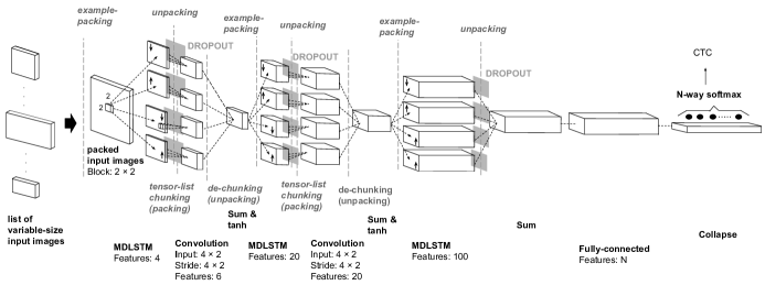
Figure 1: Network model structure, adapted from [2], with places where packing/unpacking are applied for efficient computation.

II Overview

The term handwriting recognition is sometimes used to cover the whole range of sub-tasks associated with handwritten text, including for example word spotting [11, 12], which groups word images into clusters of similar words. In the context of this publication however, we use neural handwriting recognition (NHR) to refer specifically to the task of creating text output from handwritten text images. More precisely: 1) the input is in the form of (cut-out) images of handwritten text, i.e. word-strips or line-strips, 2) output is in the form of character or word-sequences, 3) a deep learning model is used to produce sequences of character probabilities, this is used in combination with connectionist temporal classification (CTC) [13] and the associated loss-function, 4) the whole system is trained end-to-end with mini-batches of labeled examples, using back-propagation and other standard deep learning techniques. Our model is chosen to be almost identical to the one used in [2], with the difference that we share the last, fully-connected layer across directions. Figure 1 shows the model structure. It also includes the places where example-packing can be applied, to process variable-sized examples more efficiently using minimal padding. Example-packing is discussed in section V. In Appendix C we discuss details regarding the software that has been used in this work.

III Leaky LP cells: a stable version of MDLSTMs

MDLSTMs [6] are the multi-dimensional extension of long short-term memories (LSTMs). In this paper we focus on the 2-dimensional version of MDLSTMs, which is the version used for NHR. For readers unfamiliar with the details of this type of network cells, it is helpful to make a comparison with one-dimensional recurrent neural networks (RNNs) and LSTMs [14], see Figure 3. For simple 1D-RNNs there is one input and hidden unit, and one output. For MDLSTMs this is extended with an additional input state and output state. In contrast, for 2-D-MDLSTMs there are two neighboring predecessor cells in a conceptual 2D grid of cells used for computation. Each neighbor provides a pair of of $\langle$hidden, state$\rangle$ inputs, with the other input called cell input coming from the computed cell, as in the 1D case. Furthermore, stacking the output of four different MDLSTMs, one for each possible direction the 2-D grid can be scanned, yields a 4-directional 2-D-MDLSTM. This version is the one typically used for NHR. Figure 4(a) shows the computational graph for MDLSTMs. A crucial role is played by two forget gates used to weigh and then combine the states $S_{1}$ and $S_{2}$, obtained as inputs from the two predecessor cells. The value of these gates is in the range zero to one, and here lies a problem. When the sum of the gate activations becomes larger than one, the absolute values of the state entries, i.e. the norm of the state, can grow over time. As thoroughly discussed in [10] and confirmed in our own experiments, this is a real problem and not just a theoretical one. States can grow rapidly over time, and even become infinity, and gradient clipping cannot fix this either. A naive solution would be to simply multiply the output of both gates by a factor 0.5, guaranteeing that the combined gate activation never exceeds 1. But [10] note that while fixing the instability problem, this causes a new problem by making it impossible for the cell to preserve state, that is remember, over a long time. Therefore, they proposed a more rigorous solution, introducing so-called lambda-gates that produce a weighted sum of the inputs, with the weights being predicted by the gate and summing to one, see Figure 4(b). This solves the severe problems of MDLSTM instability, as also reported by [3], while retaining the crucial ability to preserve state over a long time.

Based on the idea of lambda-gates, multiple variants of stable MDLSTM cells are possible, as discussed in [10], with the best performing one being the Leaky LP cell, but all of them yielding solid results. In this work, we use a slight variant of the Leaky LP cell: the previous memory state is used in place of the newly computed memory state as (memory) input to the two output gates. This variant yielded faster learning and superior results in our experiments.

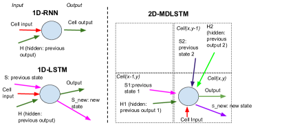
Figure 2: 1-D LSTM versus 2-D-MDLSTM computational structure

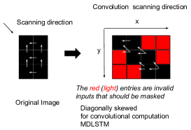
Figure 3: The input-skewing trick.

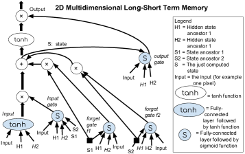
(a) 2-D MDLSTM computational graph.

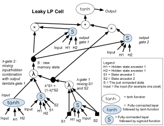
(b) 2D Leaky LP cell computational graph: with $\lambda$ gates.

Figure 4: Computational graph for MDLSTM and its stable variant Leaky LP cell.

IV Parallelizing the computation

To make training and application of MDLSTM-based NHR models computationally feasible, parallelization is crucial. Parallelization over the batch computation is the simplest form of parallelization, and is available without any additional effort in most deep learning frameworks. However, due to the large amount of memory required by each example and its MDLSTM representations, it is typically not possible to drastically increase the batch size as a simple way to increase parallelization. The exact batch size possible for NHR will depend per problem and setup, but in practice very large batch sizes are not possible. For this reason, additional other forms of parallelization should be considered and implemented wherever possible.

IV-A Parallel column computation using the input-skewing trick

The next optimization with large impact is the parallelization of MDLSTM computation within image columns, introduced by [9], increasing the level of parallelism by a factor as large as the example height. Notably, a similar trick was discovered independently by [3], but their variant relied on low-level implementation rather than leveraging existing tools, particularly efficient implementations of convolution, within deep learning frameworks. As explained in section III, computation of 2-D MDLSTMs can be modeled as a grid of computational “cells”, whereby each cell takes context input on two neighboring ancestor cells, one above and one on the left (as defined by the scanning direction). Figure 3 shows what we will call the input-skewing trick: each of the $n-1$ image rows $r_{i},i\in[2,n]$ is shifted with an increasing number of $i-1$ pixels. The results is a diagonally skewed input image that can be applied for efficient computation of the MDLSTM using convolution. The input-skewing trick transforms the original input into a row-shifted version. This produces a conceptual grid of computational cells, whereby each column of cells depends only on cells in the previous column. The skewed input image and corresponding computational grid, contains cells that correspond to valid/invalid inputs, marked by black/red squares in Figure 3. A binary mask tensor with ones/zeros for the valid/invalid cells is used to mask invalid inputs during computation. Skewed input image plus mask thereby enable fast computation with framework-native convolutional layers, without low-level programming.

IV-B Convolutions with Grouping

Another technique to further increase parallelism, relevant to deep learning frameworks with dynamic graph definition including PyTorch, is to make use of convolutions with grouping. While conceivably this technique has been used in other domains, to the best of our knowledge, it has not been proposed for NHR. In convolution with grouping, the computation is partitioned into $m$ input groups and $n$ output groups. Each of the $n$ outputs is only connected to the nodes of one of the $m$ input groups, whereby $n$ must be an exact multiple of $m$. The output of a convolution network with $m$ input and $n$ output groups is the same as for $m\times n$ separate networks, each with $\frac{1}{m}$th of the inputs connected to one $\frac{1}{n}$th of the outputs; but the difference is that these $m\times n$ grouped computations are performed in parallel rather than sequentially.

Figure 4(a) shows the computational graph for 2D-MDLSTM computation. Taking into account the structure of the graph, there are three main observations that enable optimization of MDLSTM computation (and analogously Leaky LP cell computation), using convolutions with grouping:

1. The computation of one MDLSTM cell / a column of MDLSTM cells (using the input-skewing trick), can be divided into a set of operations that are mutually independent, and hence can be computed in parallel.

2. Most of the computations rely on the current pixel input and/or the ancestor hidden and memory states as inputs.

3. Even when the inputs differ, it remains possible to parallelize multiple computations using a single convolution with grouping. This is done by having multiple input groups in addition to multiple output groups. Finally, in cases where the number of outputs per input differs per input, this can be solved by replicating some of the inputs multiple times. This gets around the typical restriction that $n$ must be an exact multiple of $m$.

In the concrete case of 2D-MDLSTM computation (see Figure 4(a)), there are five matrix computations necessary to get input activations for the input node, input gate, two forget gates, and output gate. Since these input activation computations depend only on the input, either an image or input from the previous network layer, they can all be computed in parallel using a 2-dimensional convolution. This convolution is of size $1\times 1$ for both filters and stride, to avoid overlap between convolution kernel applications. It is then further parallelized using grouping, in this case with just one input group and five output groups. Convolutions with grouping are similarly applied to parallelly compute the multiple tensors that use the same hidden or memory states as the input. Details are given in Appendix A.

IV-C Example-list based multiple-GPU training

Parallelization over multiple GPUs is another way to further increase the speed of computation. This type of parallelization is typically supported natively in deep learning frameworks, for example in PyTorch there is a method DataParallel that supports it. However, the problem with DataParallel is that it only works with tensors of the same size. Essentially it expects a data and label tensor with uniform dimensions, so that it can divide these into a number of chunks, and provide one $\langle$data, label$\rangle$ chunk pair to each GPU. For different-sized example images, which are the norm in NHR, this approach breaks down. To fix it, we create a custom DataParallel that accepts the data to come in the form of a list of variable-size image tensors. The list is then split into approximately equal-size sub-lists, and a data sub-list with corresponding label sub-tensor is provided to each GPU.

V Example-Packing

MDLSTMs parallelization is restricted by the inherent recurrent dependency upon previous hidden and memory-states. In the case of NHR based on line-strips, parallelization within the computations for a line-strip pixel column is possible. But parallelization across pixel columns is not, because of the computational dependencies. Therefore, it is desirable to exploit the ways of parallelization that are possible to their limit. One obvious way to increase parallelization is to increase the batch size. But this approach, when naively applied, requires all the examples to be padded to the same size. For handwriting line-strips or word-strips, which are naturally of different dimensions, this approach is computationally wasteful in two ways.

1. The padding pixels use up a lot of wasted computation.

2. This wasted computation coincides with memory waste: the space required for the padding could have been used to fit in more real pixels, needed for the end result.

The question is: can we overcome the limitation that all examples need to be of the same size, while still respecting the constraints of efficient GPU computation? The conclusion is, we can, by using a combination of:

1. Tiling together examples together to using a greedy space-filling algorithm to use the available space as much as possible.

2. Separating pixels between the tiled examples.

3. Binary masking to block the hidden-state and memory-state input from predecessor cells that are not valid input cells but padding cells or separator cells according to the binary mask.

This is best explained by an example. Figure 5(a) shows a set of artificial, packed examples, and Figure 5(b) the corresponding mask.

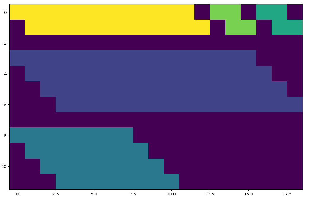
(a) Packed artificial examples

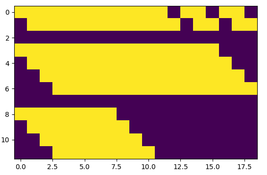
(b) Corresponding binary mask

Figure 5: Packed artificial data example and corresponding mask.

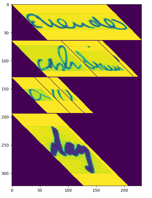
(a) Packed IAM words data example

(b) Packed IAM lines data example

Figure 6: Packed IAM words and lines data

Note that examples of the same height are arranged in a single row. This is a requirement for allowing column-parallelized MDLSTM computation with the input-skewing trick. Furthermore, note that one row of pixels is added between every pair of examples. These rows of pixels get skewed diagonally along with the input images, as a result of the input-skewing trick. Figure 6(a) shows the result of example-packing for IAM data examples, consisting of IAM word-strips. Here, while there is still quite some padding, a large part of it is caused by the input-skewing trick. But note that while not perfect, packing saves out a lot of padding. Without it, every example needs to be padded to the largest width and height dimensions occurring in the mini-batch, in this case making all examples as wide as the first row example and as high as the last row example. Finally, one may expect that working with line-strips instead of word-strips, which for many dataset, such as IAM, is the default, the differences between the sizes of the image strips are smaller singe the word-lengths average out. This is indeed partly true, see Figure 6(b), however, at the same time the remaining height-differences imply that example-packing can still yield significant savings, predominantly in the height dimension.

V-A Efficient packing

With the basic principles behind example-packing explained, the next question is how to find a packing that optimally uses the space, tiling the examples in a mini-batch such a way to add as little padding as possible. First note that there is no need that the dimensions across mini-batches are the same, and this fact is exploited in our approach. Second, note the earlier mentioned constraint: to allow efficient skewing and un-skewing of rows of examples, all examples in the row must be of the same height. This motivates a four step approach: 1) bucket the examples by height, 2) pack the examples in each height bucket, filling up rows, by repeatedely and greedily adding the widest still fitting example, 3) tiling the examples first within packed rows, then across rows, adding separating pixels in between, 4) applying the input skewing trick to create a skewed version of the resulting packed tensor and mask. In Appendix B we provide pseudocode for the packing algorithm.

Packing is performed just before the computation of each MDLSTM layer, based on a list of input tensors for that layer. After the MDLSTM activations are computed on the packed tensors, unpacking is performed on these activations. Figure 1 indicates these places where packing/unpacking is apllied in the network. Unpacking is packing in reverse, and consists of the following two steps: 1) the inverse of the input skewing trick is performed to restore the tensor format before skewing, 2) using the original example indices corresponding to the packed examples and their sizes, the activations per input example are extracted, while discarding parts of the activations corresponding to separating pixels in the input.

V-B Packing for block-strided convolution layers

Block-strided convolutional layers are convolutional layers with a stride width and height (“block-size”) corresponding to the size of the convolution kernel, such that there is no overlap in input for different kernel applications. These layers layers are used to merge the output of MDLSTM layers and decrease resolution. They require their own pre- and post-processing algorithms to allow efficient processing of input lists obtained from MDLSTM layers. These two algorithms perform a sort of simplified packing/unpacking. The tensor-list chunking (packing) algorithm chunks a list of input tensors of different sizes into blocks of given size, in our case the block-stride of the block-strided convolution layer. The chunking produces for each tensor a list of blocks, and stacks all these blocks on the batch simension. This stacked block tensor can be processed very efficiently by a standard 2-D convolution layer. After computation of the convolutional features, using the size of the tensors in the original input list, a de-chunking algorithm (un-packing) concatenates the output activation blocks again together. This application of tensor-list chunking/de-chunking to block-strided convolution is indicated in Figure 1 as well. The thus parallely computed result list is equal to what would be obtained if the block-strided convolution was computed for each input tensor separately and the result tensors collected in a list.

VI Effective Optimization

We found the use of gradient clipping, particularly the technique proposed in [15], which constitutes rescaling of the gradient to normalize the gradient norm, to be necessary to achieve stable learning. Whereas the use of Leaky LP cells was another crucial component, in our experience gradient clipping was still needed on top of that to obtain good results. In addition to that, we found that the learning rate, max norm for gradient clipping and optimizer needed to be chosen well together. Unfortunately, this is mostly an empirical matter, in which previous literature can at most help. We obtained good results, using the Adam optimizer [16] with an initial learning rate of 0.005, and gradient clipping using a maximum gradient norm of 10 to be effective. We used the technique of [17] to improve Adam, by halving the learning rate and resetting the Adam state when the validation scores (WER and CER) got worse, resuming training from the best last model. Following [3], we trained for a maximum of 80 epochs, after which we selected the best performing model on the validation-set, and used this model to evaluate on the test-set.

(a) Character Error Rate (CER)

(b) Word Error Rate (WER)

(c) Average CTC Loss per minibatch

Figure 7: Results on the IAM validation set for MDLSTM NHR networks trained with or without dropout. For these results, decoding is done using a beam-search decoder without language model.

VII Experiments

VII-A Dataset

We perform experiments on the IAM-database [18], which is an English multi-writer handwriting dataset based on material from the Lancaster-Oslo/Bergen (LOB) corpus. We chose this dataset as it is one of the most frequently used benchmark datasets in the field, and a such facilitates easy comparison to other works including [2, 3, 7]. As such, during our reimplementation of MDLSTM-based NHR models from scratch, the dataset was invaluable for testing where we stood with our system in comparison to earlier work. The IAM database is of moderate size. It contains material of 657 different writers, and is partitioned into subsets for validation, training and testing of 161, 966 and 2 915 lines. This data split corresponds to the split of the IAM (lines) dataset used in [2], [3] and [7]. For the IAM words dataset we used the same split files, and obtained subsets for training, validation and testing of 55079, 8895 and 25920 words. Unfortunately, somehow these sizes for the words dataset do not match the word-set sizes for training, validation and testing reported in [2] (80421, 16770, 17991) even though they were derived from the same data spit files. This makes an exact quality comparison with [2] for the word recognition systems not possible. However, since our main quality comparison is on line recognition, this is not a major problem, and we leave further investigation of this issue for future work. In combination with the IAM dataset, we use a domain-specific language model trained on material from the (unused parts of the) LOB corpus and the Brown corpus.

VII-B Results

Figure 7 shows graphs tracking the model performance across training progress, in addition Table I shows the results on the validation and test-set, using the best performing validation model and applying it to the test-set. Figure 7(a) and 7(b) show the character error rate (CER) and word error rate (WER) scores on the validation set, without use of a language model during decoding; and Figure 7(c) shows the average CTC loss per epoch. From these graphs, and the table, a few observations can be made. First, the models trained using dropout outperform these without dropout. Second, whereas in case dropout is used the larger model with MDLSTM layer sizes of 4, 20 and 100 performs best, without dropout this model performs worse than the smaller model with MDLSTM layer sizes of 2, 10 and 50. This is in line with what has been reported earlier in the literature, i.e. in [2]. Third, the models without dropout have a CTC loss graph that keeps going down, whereas the CER and WER start to increase (i.e. worsen) again after a certain number of epochs, indicating over-fitting. In contrast, the CTC loss graphs for the models that use dropout flatten out faster after some point, whereas the quality of the models as measured by CER and WER for these models keeps increasing nearly till the end. Last, both systems with dropout not only give final better results, but also improve faster than the models without dropout, with the largest model with dropout showing a markedly faster improvement towards a decent system than all other systems. In summary, these graphs show that dropout is highly effective both in delivering superior results, as well as in our case in delivering them faster.

Table II shows a comparison of our best models against the results by [2] and [3] in the literature. Comparing to the results of [2], it can be noted that our best system using dropout is still slightly outperformed by theirs, but the difference is small. The remaining difference might still be explained by the fact that they use a form of curriculum learning, training first on the words and then on the lines, as well as using a different optimizer.

We mostly followed [3] in our training approach, not using curriculum learning and using Adam instead of SGD (or RMSPRob) as an optimizer. The lower performance we obtain in comparison to [3] is explainable from the our different network structure, which is chosen almost identical as [2]. As our work focusses on proposing computational gains, which apply also for even fancier networks, for example adding max-pooling layers and layer normalization, we consider the fact that in terms of recognition accuracy our model performs slightly below state-of the-art not to be a big problem.

Table III shows our results on IAM words and the reported results on IAM words from [2]. Our results on IAM words without vocabulary are worse than those of [2] in this setting. However, as discussed before, these scores cannot really be compared. Using the same dataset split as for IAM lines, our training set became considerably smaller than the size reported in [2], which probably explains the score-differences.

TABLE I: Recognition quality results on the IAM lines validation-set and test-set.

	validation		test
System	WER	CER	WER	CER
Leaky LP Cell [2,10,50], no dropout	43.8	13.9	52.2	18.8
+ Vocabulary and LM	15.6	6.4	22.1	9.9
Leaky LP Cell [4,20,50], no dropout	47.4	15.7	54.6	20.4
+ Vocabulary and LM	19.1	8.9	25.1	12.9
Leaky LP Cell [4,20,50], dropout	38.4	11.3	44.0	14.5
+ Vocabulary and LM	17.7	7.8	18.6	8.3
Leaky LP Cell [4,20,100], dropout	33.9	9.8	40.8	12.9
+ Vocabulary and LM	15.5	6.4	15.9	6.6

TABLE II: Comparison to literature results on IAM lines.

	validation		test
System	WER	CER	WER	CER
Leaky LP Cell [4,20,100], dropout	33.9	9.8	40.8	12.9
+ Vocabulary and LM	15.5	6.4	15.9	6.6
Pham et.al (2014), no dropout	36.5	10.4	43.9	14.4
+ Vocabulary and LM	12.1	4.2	15.9	6.3
Pham et.al (2014), dropout	27.3	7.4	35.1	10.8
+ Vocabulary and LM	11.2	3.7	13.6	5.1
Voigtlaender et.al (2016)	7.1	2.4	9.3	3.5

TABLE III: Recognition quality for IAM words and literature results using a larger training set (see section VII-A).

	validation		test
System	WER	CER	WER	CER
Leaky LP Cell [4,20,100], dropout	33.58	14.11	42.05	19.15
+ Vocabulary	20.12	10.42	25.66	14.29
Pham et.al (2014), dropout	—	—	31.44	14.02

TABLE IV: Memory and time usage for models with and without example-packing, with batch sizes chosen the maximal possible given the observed maximum GPU memory usage.

Preparation of batch examples	batch size	time per epoch (HH:MM: SS)	examples per second	max GPU1 memory use (MB)	max GPU2 memory use (MB)
IAM lines
batch-padding	8	07:24:06	0.243	10824	10675
example-packing	12	05:04:45	0.355	10694	10780
IAM words
batch-padding	20	06:26:48	2.38	11074	11144
example-packing	200	00:58:22.	16.1	10827	10849

VII-C Impact of packing on the training time

In this section we show the impact of packing on the training times in both the (IAM) line-recognition and (IAM) word-recognition scenario. In the setting were packing is not used, we instead use a strategy we will call last-minute batch-padding (LMBR), padding examples for each batch (on-the-fly) to the maximum height and width occurring within that batch. LMBR is already a faster baseline than padding all examples within the training set to the same maximum height and with, which is a simple but computationally wasteful strategy.

Table IV shows the time consumed per epoch, examples per second and maximum GPU memory usages for identical models that were trained with or without example-packing. For these experiments, we used our best performing model with MDLSTM layers of sizes 4, 20 and 100 plus dropout, while the batch sizes were chosen to be maximal given the peak GPU memory consumption for the setting. This yielded for line recognition batch sizes of 8 when no packing was used, and 12 when it was used and for word recognition batch sizes of 20 when no packing was used, and 200 when it was used As can be seen, these settings yield to similar maximum memory usage, and neither of the batch sizes could be further increased without running out of the total available GPU memory (11178 MB).

For line recognition, looking at the times per epoch or examples per second, it can be observed that using packing the same computation can be done in 69% of the time used without packing. When testing on line strips, the savings come mostly from avoiding the need to pad al examples within a batch to the same height, as in this case the width differences between words average out to a large extent. Even so, already in this settings packing makes a noticeable difference. Looking at word recognition next, the speed improvements are more drastic. Whereas without packing, one epochs takes about six and a half hours, with packing it takes only about an hour, thanks to the major gains in efficiency packing yields in this setting, indicated by the much larger possible batch size of 200. This major speedup, by a factor 6.6, is even relevant for models which use convolutional layers to replace MDLSTMs [7]. Since while these systems are perhaps more efficient to begin with, they still waste a lot of computation on padding and could therefore benefit from packing, with some adaptations for the changed network structure.

Are variable batch sizes an alternative to packing?
Whereas in case of word-recognition, without packing on average about 75% of the input pixels consists of padding, this factor four saving does not explain the even larger difference in possible batch sizes. The reason that the maximum batch size using packing (200) is ten times larger rather than “just” four times larger than the size without packing (20), is that for the maximum possible batch size the “worst-case” batch counts, and not the average batch. That is, a single batch with one very high and one very wide example creates a peak in memory usage, and the batch size must be chosen to allow this peak value to still fit in the maximal GPU memory. In contrast, when packing is used (and padding mostly avoided), the fluctuation in effective input size and consequently GPU memory usage is much smaller. This suggests that as a partial alternative to packing, some savings could also be made by using a variable batch size, which resizes based on the size of the examples within the batch. However, this gives its own complications in terms of efficient data loading. It may also require additional measures to be taken in order to keep stable learning. Finally, note that saving out most of the factor-four blowup in size because of padding using example-packing is by itself substantial, and this saving can only be realized by packing, not by using variable batch sizes.

VIII Discussion

While the packing techniques as applied in this paper are specific to MDLSTMs, the general principle of efficient packing and unpacking of variable-size examples provided as a list is general enough to be adapted for large speed improvements of many deep learning models that work with variable-sized inputs. Notably, the tensor-list chucking algorithm as discussed in section V-B is itself an illustration of how the idea first developed for MDLSTM layers was then adapted for convolution layers with non-overlapping strides as well. Whereas the generalization of this algorithm to general convolution layers is slightly more complex than the algorithm described here, it is of a similar form. In future work we would like to further generalize the principle of packing, so that more different network types dealing with variable-size inputs can benefit from it.

IX Conclusion

We presented several new methods that can help to drastically increase the speed of deep learning models using MDLSTMs. One of these techniques, example-packing, achieved a factor 6.6 speed improvement on word-based handwriting-recognition, by avoiding wasted computation on padding. Our methods were thoroughly tested on a MDLSTM-based implementation of state-of-the-art neural handwriting recognition models implemented with PyTorch.

Appendix

IX-A Further application of convolutions with grouping

For computing fully-connected layers that take input from hidden states and memory states, convolutions with grouping are applied to increase parallelization. There are five matrix computations necessary for each of the two hidden states $H_{1}$ and $H_{2}$, and three for each of the memory states $S_{1}$ and $S_{2}$. Since the hidden- and memory state computations have the same input dimensionality, we can all compute them using a single convolution with grouping, using replication of the input to overcome the fact that the number of output groups differs for the hidden- and memory states. Finally, we can shift the output by once cell for the second hidden- and memory state respectively, to get a vector of activations of the top ancestor states but overlayed with the activations of the left ancestor states. That way the activation tensors for the two hidden/memory states can be directly summed to combine them for further computation.

IX-B Packing Algorithm Details

Data: List of examples

Result: $t_{packed\_examples}$, $t_{masks}$: tensors, $original\_example\_indices$ : 2-D array datastructure storing the original example indices for the examples in the filled rows

$height\_buckets$ := Bucket the examples into groups of the same height ;

$packing\_rows$ := [] ; $original\_example\_indices$ = [] ; $current\_row$ := [] ; $current\_indices\_row$ := [] ;

for height_bucket $\in$ height_buckets do

       while not_empty(height_bucket) do

             $example$, $original\_example\_index$ := largest_fitting_example($current\_row$, $height\_bucket$) ;

             if example != None then

                   $current\_row$.append(example) ; current_indices_row.append(original_example_index) ;

                  

             else

                   # Current row is full, start a new row

                   $packing\_rows$.append(current_row) ; $original\_example\_indices$.append(current_indices_row) ;

                   $current\_row$ = [] ; current_indices_row = [] ;

            

      

$t_{packed\_examples}$ := concatenate_packing_rows_adding_separation_pixels($packing\_rows$) ;

$t_{masks}$ := create_mask($t_{packed\_examples}$) ; # all example indices replaced by 1, and all separator pixels replaced by 0

$t_{packed\_examples\_skewed}$ := apply_input_skewing($t_{packed\_examples}$) ; $t_{masks\_skewed}$ := apply_input_skewing($t_{masks}$) ;

return $t_{packed\_examples\_skewed}$, $t_{masks\_skewed}$, $original\_example\_indices$

Algorithm 1 Packing Algorithm

IX-C Experimental details and source-code

All our experiments were done using PyTorch. We used two NVIDIA GEFORCE^® GTX 1080 graphic cards to run our experiments. In our work, for implementing ctc-loss, we used PyTorch bindings for warp-ctc [19] by Baidu research. Our version of the code, was forked and slightly adapted from the one by Sean Naren and others. Additionally we used a slightly adapted version of the ctc beam-search decoder for PyTorch, developed by Ryan Leary and others. This decoder supports KenLM [20] word-based n-gram language models, which we use in our experiments. The rest of our source-code is intended to be made available together with a peer-reviewed publication of the work.

References

- [1] T. Bluche, H. Ney, and C. Kermorvant, “Feature extraction with convolutional neural networks for handwritten word recognition,” 2013 12th International Conference on Document Analysis and Recognition, pp. 285–289, 2013.
- [2] V. Pham, T. Bluche, C. Kermorvant, and J. Louradour, “Dropout improves recurrent neural networks for handwriting recognition,” Arxiv https://arxiv.org/abs/1312.4569v2), pp. 1–6, 2016.
- [3] P. Voigtlaender, P. Doetsch, and H. Ney, “Handwriting recognition with large multidimensional long short-term memory recurrent neural networks,” In proceedings of the International Conference on Frontiers in Handwriting Recognition (ICFHR), pp. 228–233, 2016.
- [4] U.-V. Marti and H. Bunke, “Hidden markov models,” 2002, ch. Using a Statistical Language Model to Improve the Performance of an HMM-based Cursive Handwriting Recognition Systems, pp. 65–90.
- [5] S. Bengio, A. Vinciarelli, and H. Bunke, “Offline recognition of unconstrained handwritten texts using hmms and statistical language models,” IEEE Transactions on Pattern Analysis & Machine Intelligence, vol. 26, pp. 709–720, 2004.
- [6] A. Graves, S. Fernández, and J. Schmidhuber, “Multi-dimensional recurrent neural networks,” in ICANN (1), ser. Lecture Notes in Computer Science, vol. 4668. Springer, 2007, pp. 549–558.
- [7] J. Puigcerver, “Are multidimensional recurrent layers really necessary for handwritten text recognition?” in 14th IAPR International Conference on Document Analysis and Recognition, ICDAR 2017, 2017, pp. 67–72.
- [8] M. Carbonell, M. Villegas, A. Fornés, and J. Lladós, “Joint recognition of handwritten text and named entities with a neural end-to-end model,” CoRR, vol. abs/1803.06252, 2018.
- [9] A. Van Den Oord, N. Kalchbrenner, and K. Kavukcuoglu, “Pixel recurrent neural networks,” in Proceedings of the 33rd International Conference on International Conference on Machine Learning - Volume 48, ser. ICML’16, 2016, pp. 1747–1756.
- [10] G. Leifert, T. Strauß, T. Grüning, W. Wustlich, and R. Labahn, “Cells in multidimensional recurrent neural networks,” Arxiv https://arxiv.org/abs/1412.2620), pp. 1–35, 2014.
- [11] T. M. Rath and R. Manmatha, “Word spotting for historical documents,” INTERNATIONAL JOURNAL ON DOCUMENT ANALYSIS AND RECOGNITION, vol. 9, pp. 139–152, 2007.
- [12] A. Fischer, A. Keller, V. Frinken, and H. Bunke, “Lexicon-free handwritten word spotting using character hmms,” Pattern Recogn. Lettters, vol. 33, no. 7, pp. 934–942, 2012.
- [13] A. Graves, S. Fernández, F. Gomez, and J. Schmidhuber, “Connectionist temporal classification: Labelling unsegmented sequence data with recurrent neural networks,” in Proceedings of the 23rd International Conference on Machine Learning, 2006, pp. 369–376.
- [14] S. Hochreiter and J. Schmidhuber, “Long short-term memory,” Neural Computation, vol. 9, no. 8, pp. 1735–1780, 1997.
- [15] R. Pascanu, T. Mikolov, and Y. Bengio, “On the difficulty of training recurrent neural networks,” in Proceedings of the 30th International Conference on Machine Learning, vol. 28, no. 3, 2013, pp. 1310–1318.
- [16] D. P. Kingma and J. Ba, “Adam: A method for stochastic optimization.” in Proceedings of the 3rd International Conference on Learning Representations (ICLR), 2014, pp. 1–15.
- [17] M. Denkowski and G. Neubig, “Stronger baselines for trustable results in neural machine translation,” in Proceedings of the First Workshop on Neural Machine Translation. Association for Computational Linguistics, 2017, pp. 18–27.
- [18] U.-V. Marti and H. Bunke, “The iam-database: an english sentencedatabase for offline handwriting recognition,” International Journal on Document Analysis and Recognition, vol. 5, no. 1, pp. 39–46, 2002.
- [19] D. Amodei, S. Ananthanarayanan, R. Anubhai, J. Bai, E. Battenberg, C. Case, J. Casper, B. Catanzaro, Q. Cheng, G. Chen, J. Chen, J. Chen, Z. Chen, M. Chrzanowski, A. Coates, G. Diamos, K. Ding, N. Du, E. Elsen, J. Engel, W. Fang, L. Fan, C. Fougner, L. Gao, C. Gong, A. Hannun, T. Han, L. V. Johannes, B. Jiang, C. Ju, B. Jun, P. LeGresley, L. Lin, J. Liu, Y. Liu, W. Li, X. Li, D. Ma, S. Narang, A. Ng, S. Ozair, Y. Peng, R. Prenger, S. Qian, Z. Quan, J. Raiman, V. Rao, S. Satheesh, D. Seetapun, S. Sengupta, K. Srinet, A. Sriram, H. Tang, L. Tang, C. Wang, J. Wang, K. Wang, Y. Wang, Z. Wang, Z. Wang, S. Wu, L. Wei, B. Xiao, W. Xie, Y. Xie, D. Yogatama, B. Yuan, J. Zhan, and Z. Zhu, “Deep speech 2: End-to-end speech recognition in english and mandarin,” in Proceedings of the 33rd International Conference on International Conference on Machine Learning - Volume 48, ser. ICML’16, 2016, pp. 173–182.
- [20] K. Heafield, “KenLM: faster and smaller language model queries,” in Proceedings of the EMNLP 2011 Sixth Workshop on Statistical Machine Translation, Edinburgh, Scotland, United Kingdom, July 2011, pp. 187–197.