Fast roughness minimizing image restoration under mixed Poisson-Gaussian noise

Abstract

Image acquisition in many biomedical imaging modalities is corrupted by Poisson noise followed by additive Gaussian noise. While total variation and related regularization methods for solving biomedical inverse problems are known to yield high quality reconstructions in most situations, such methods mostly use log-likelihood of either Gaussian or Poisson noise models, and rarely use mixed Poisson-Gaussian (PG) noise model. The work of Chouzenoux et al. deals with exact PG likelihood and total variation regularization. This method adapts the primal-dual approach involving gradients steps on the PG log-likelihood, with step size limited by the inverse of the Lipschitz constant of the gradient. This leads to limitations in the convergence speed. Although ADMM methods do not have such step size restrictions, ADDM has never been applied for this problem, for the possible reason that PG log-likelihood is quite complex. In this paper, we develop an ADMM based optimization for roughness minimizing image restoration under PG log-likelihood. We achieve this by first developing a novel iterative method for computing the proximal solution of PG log-likelihood, deriving the termination conditions for this iterative method, and then integrating into a provably convergent ADMM scheme. The effectiveness of the proposed methods is demonstrated using restoration examples.

Keywords Image Restoration, Maximum likelihood estimator (MLE), Alternating direction method of multipliers (ADMM), Poisson-Gaussian noise, Total variation, Regularization

1 Introduction

The restoration of images from blur and noise is an important problem with applications in microscopy [1],[2], [3] astronomy[4], [5] and other sciences. Image restoration is often posed as MAP estimation problems constructed using a wide variety of assumptions on prior probability of the underlying image, and conditional probability of measured pixel values given the degradation model. Various priors such as sparsity in wavelet domain [6], sparsity in space domain [2], sparsity of spatial derivatives [7], [8] promote different types of structures in the recovered image. The cost functionals corresponding to derivative-based priors are known as total variation functionals [8]. Initially, first order image derivative was used to construct such functionals, in which case the functionals are known as first order total variation functionals. Then it has been demonstrated that second-order total variation functionals built using second order derivatives yield better reconstruction quality [9]; in particular, the use of such functionals avoid the staircase effect [10] caused by first-order functionals.

The data fitting (fidelity) term is essentially the negative logarithm of the conditional probability of the measured pixel value given the ideal measurable pixel value; it is also known as likelihood function, and it indeed accounts for the probability distribution of the random process that generates the noise in the measurement device. Most commonly used data fitting models are Gaussian and Poisson because of their simplicity in computation and modelling. However, the degradation caused in image capturing devices such as EM-CCD or CMOS devices is appropriately modeled by a Poisson process signifying the photon counting followed by the additive Gaussian noise accounting for thermal errors [5]. This motivates image restoration under the mixed Poisson-Gaussian model (PG) model. This model is especially relevant in case of biological [11] and astronomical imaging [5]. This paper aims to develop a faster and practical algorithm for image restoration using the MLE-based data fitting term involving exact Poisson-Gaussian (PG) likelihood and the class of convex regularization functionals that have a closed form proximal solution [12].

Most of the published works in image restoration involving PG likelihood function employ some approximation such as Generalized Anscombe Transform (GAST) [13], [14, 15, 3] or (shifted) Poisson approximation [16, 17]. GAST, a variance stabilizing transform, is a non-linear (square root) transform which is applied on the measurements in order that the noise statistics in the measurements are well approximated by a Guassian distribution. The approximation is closer when the mean of the Poisson random variable is high [18]. In [14], a two stage de-noising approach is developed using GAST. In the first stage, the measured data is applied with Anscombe Transform to ‘gaussianize’ the data, and in the second stage a sparsity driven iterative algorithm is employed to obtain the final solution. In shifted Poisson approximation [16, 17], the measurements are added (shifted) with variance of Gaussian random variable, in order that noise in the result is approximated by a Poisson distribution. This approximation performs well when the Gaussian noise variance is low. The work of Marnissi et al. [17] also considers GAST along with shifted Poisson under Bayesian framework. This approach relies on joint estimation of the signal and the regularization parameter. Gao et al. [19] presented an interesting approach which models the Poisson-Gaussian likelihood as a mixture of Gaussians. The prior considered was Markov Random field prior. The de-noising/de-blurring problem in the approach was formulated as a joint estimation of prior parameters, likelihood parameters and the image variable. The restoration results from these algorithms are not as good as the ones obtained using exact PG likelihood [20], and there is a scarcity of algorithms considering exact PG likelihood term with TV regularization. Furthermore, the methods that use the exact PG likelihood [4, 20] either has issues in convergence or do not use total variation based regularization functionals. Specifically, the scaled gradient algorithm [4] does not have any convergence guarantees, and also it does not consider any regularization term.

Chouzenoux et al. [20] have proposed a rigorous and general approach for image restoration under PG noise model with total variation. Its generality stems from the fact that, the approach can be extended to any regularization. However, the the step-size of the iterative method is restricted to be lower than the inverse of the Lipschitz constant of the gradient of the log-likelihood functional. Hence, the convergence is typically slow.

ADMM based methods are attractive in the sense that they do not face any limitation in the step-size, and hence are typically faster than methods that use gradient-based stepping. An ADMM method applied on a composite cost functional is comprised of a series of minimization steps that cycles through the sub-functionals of the composite cost functional. The original framework [21] requires that the sub-functionals in each cycle has to be minimized exactly. This framework has been used for image restoration under Poisson noise and under Gaussian noise, and have been shown to be faster than other state-of-the-art methods [22, 23]. As the PG log-likelihood is complex, exact minimization of corresponding sub-functional is not possible in the present problem. Fortunately, a recently proposed modified ADMM framework allows inexact minimization of the sub-functionals in the ADMM cycles [24]. In this paper, we adapt this framework for the problem of image restoration using convex regularization functionals under the PG noise model. Our contributions are the following:

• We propose an iterative method for minimizing the sub-functional corresponding to PG log-likelihood, with proof of convergence.

• We derive termination conditions for the above-mentioned iterative scheme such that it can be integrated into the modified ADMM framework of Eckstein et al. [24].

In Section 2, we will review the ADMM applied on the problem of roughness minimizing image restoration (subsections 2.1 and 2.2). We will also review the modified framework of Yao and Eckstein, which enables solving image restoration under Poisson-Gaussian noise model (referred as PG image restoration hereafter) by means of ADMM approach. Further, we identify the computational problems to be solved for making the modified ADMM framework applicable to PG image restoration (subsection 2.3). Section 3 solves these computational problems, which is the primary contribution of this paper. Experimental results are given in Section 4. This work is an extension of the work we presented in [25], where we proposed the computational algorithm without convergence proof.

2 Roughness minimizing image restoration under Poisson-Gaussian Noise by ADMM

2.1 The cost function

Let $\boldsymbol{g}$ and $\boldsymbol{m}^{\prime}$ be the vectors containing the pixels of original and measured images respectively in a scanned form. Let $\boldsymbol{H}$ be matrix equivalent of blurring. The measurement vector $\boldsymbol{m}^{\prime}$ differs from the ideal measurement $\boldsymbol{H}\boldsymbol{g}$ by noise. Let ${F}_{\scriptscriptstyle M}(\boldsymbol{H}\boldsymbol{g},\boldsymbol{m}^{\prime})$ be the data-fitting cost functional, which is essentially the negative log of the likelihood of the noise process. In other words, ${F}_{\scriptscriptstyle M}(\boldsymbol{H}\boldsymbol{g},\boldsymbol{m}^{\prime})=-\log p_{\scriptscriptstyle M}(\boldsymbol{m}^{\prime}|(\boldsymbol{Hg}))$, where

$$p_{\scriptscriptstyle M}(\boldsymbol{m}^{\prime}|(\boldsymbol{Hg}))=\prod_{n}p_{\scriptscriptstyle M}((\boldsymbol{m}^{\prime})_{n}|(\boldsymbol{Hg})_{n}),$$ (1)

with $p_{\scriptscriptstyle M}((\boldsymbol{m}^{\prime})_{n}|(\boldsymbol{Hg})_{n})$ denoting the likelihood for $(\boldsymbol{Hg})_{n}$ being the ideal $n$th pixel given $(\boldsymbol{m}^{\prime})_{n}$ as the $n$th measured pixel. When the noise is assumed to be Gaussian, it is given by

$$p_{\scriptscriptstyle M}((\boldsymbol{m}^{\prime})_{n}|(\boldsymbol{Hg})_{n})=\frac{1}{\sqrt{2\pi\sigma^{2}}}\exp\left(-\frac{1}{\sigma^{2}}\left((\boldsymbol{m}^{\prime})_{n}-(\boldsymbol{Hg})_{n}\right)^{2}\right),$$

where $\sigma^{2}$ is the noise variance. When the noise is assumed to be Poisson, it becomes

$$p_{\scriptscriptstyle M}((\boldsymbol{m}^{\prime})_{n}|(\boldsymbol{Hg})_{n})=\exp(-(\boldsymbol{Hg})_{n})\frac{(\boldsymbol{Hg})_{n})^{(\boldsymbol{m}^{\prime})_{n}}}{((\boldsymbol{m}^{\prime})_{n})!}.$$

The most realistic form of noise model, which is the focus of this paper, is the mixed Poisson-Gaussian noise model. In this case, $\boldsymbol{m}^{\prime}$ and $\boldsymbol{Hg}$ are related as given below,

$$(\boldsymbol{\boldsymbol{m}^{\prime}})_{n}=\alpha\mathcal{P}((\boldsymbol{Hg})_{n})+\mathcal{N}(c,\sigma^{2}),\\$$ (2)

where $\mathcal{P}(\cdot)$ denotes the Poisson process, and $\mathcal{N}(c,\sigma^{2})$ is Gaussian process with mean $c$ and variance $\sigma^{2}$. Note that we consider $c=0$ in this paper. The corresponding likelihood is given by

$$p_{\scriptscriptstyle M}((\boldsymbol{m}^{\prime})_{n}|(\boldsymbol{Hg})_{n})=$$ (3)

$$\sum_{p=0}^{\infty}\frac{e^{-(\boldsymbol{Hg})_{n}}}{\sqrt{2\pi\sigma^{2}}}\frac{((\boldsymbol{Hg})_{n})^{p}}{p!}\exp\left(-\frac{((\boldsymbol{m}^{\prime})_{n}-\alpha p-c)^{2}}{2\sigma^{2}}\right).$$

Next, let $\boldsymbol{D}=\left[\boldsymbol{D}_{xx}^{T}\;\boldsymbol{D}_{yy}^{T}\;\boldsymbol{D}_{xy}^{T}\right]^{T}$, where $\boldsymbol{D}_{xx}$, $\boldsymbol{D}_{yy}$ and $\boldsymbol{D}_{xy}$ denote matrix equivalent of convolving the image with filters corresponding to derivative operators $\frac{\partial^{2}}{\partial x^{2}}$, $\frac{\partial^{2}}{\partial y^{2}}$, and $\frac{\partial^{2}}{\partial x\partial y}$ respectively. This means $\boldsymbol{D}_{xx},\boldsymbol{D}_{xy}$ and $\boldsymbol{D}_{yy}$ are block circulant matrices with circulant blocks corresponding to 2-D convolution with periodic boundary conditions for the filters $[-1,2,-1]$,$\left[\begin{array}[]{cc}1&-1\\ -1&1\end{array}\right]$ and $\left[\begin{array}[]{c}-1\\ 2\\ -1\end{array}\right]$ respectively. Let $\mathbf{P}_{i}$ denote the matrix with $1$s at positions $(i,1),(i+N,2),(i+2N,3)$ and zeros everywhere else. Further, let $\mathcal{E}(\mathbf{v})$ be the operator defined for the vector $\mathbf{v}=[v_{1},v_{2},v_{3}]^{T}\in\mathbb{R}^{3}$ that returns vector of Eigen values of the matrix $\left[\begin{array}[]{cc}v_{1}&v_{3}\\ v_{3}&v_{2}\end{array}\right]$. Then most second order derivative based roughness functionals fall under category of Hessian-Schatten norm [26], which can be expressed as given below,

$$F_{\scriptscriptstyle D}(\boldsymbol{D}\boldsymbol{g})=\sum_{i=1}^{N}\left\|\mathcal{E}(\boldsymbol{P}_{i}^{T}\boldsymbol{D}\boldsymbol{g})\right\|_{q},$$ (4)

where $q$ is a parameter in the range $[1,\infty]$. This functional is computationally least expensive when $q=1,2$. When $q=2$, this form becomes the well-known total variation functional. When $q=1$, the norm is known as the nuclear norm, which has been reported to yield better results.

With these definitions, the roughness minimizing image restoration amounts to computing the minimum of the following cost,

$$F(\boldsymbol{g})={F}_{\scriptscriptstyle M}(\boldsymbol{H}\boldsymbol{g},\boldsymbol{m}^{\prime})+\lambda F_{\scriptscriptstyle D}(\boldsymbol{D}\boldsymbol{g})+~F_{B}(\boldsymbol{g})$$ (5)

where $\lambda$ is the regularization parameter, and $F_{B}(\boldsymbol{g})$ is the indicator function for imposing bound constraint on the image pixel values. With $u^{\prime}$ (a positive real number) denoting largest pixel value that can be allowed in the restoration, $F_{B}(\boldsymbol{g})$ can be written as

$$F_{B}(\boldsymbol{g})=\sum_{i=1}^{N}\begin{cases}0&\mbox{if}\;0\leq(\boldsymbol{g})_{i}\leq u^{\prime},\\ \infty,&\mbox{otherwise.}\end{cases}$$ (6)

Next, we propose to modify ${F}_{\scriptscriptstyle M}(\boldsymbol{Hg},\boldsymbol{m}^{\prime})$ as given below:

$$\bar{F}_{\scriptscriptstyle M}(\boldsymbol{H}\boldsymbol{g},\boldsymbol{m}^{\prime})=\sum_{i=1}^{N}\begin{cases}-\ln(p_{\scriptscriptstyle M}((\boldsymbol{m}^{\prime})_{i}|(\boldsymbol{Hg})_{i}))&\\ \;\;\;\;\;\;\;\;\mbox{if}\;(\boldsymbol{Hg})_{i}\in[l,u],\\ \infty,&\mbox{otherwise}.\end{cases}$$ (7)

This is equivalent to imposing the constraint that the components of $\boldsymbol{Hg}$ stay within the bound $[l,u]$. First note that $0\leq l\leq u$. Secondly, $l$ can be set to zero and $u$ to $||\boldsymbol{H}||_{1}u^{\prime}$. The second result is obtained by a straight forward application of Holder’s inequality. Although, the above bounds clearly redundant because of the bound constraint on $\boldsymbol{g}$, this helps to make to ADMM iteration well-behaved. This will be explained later in Section IV.B. With this modification, the overall cost to be minimized is given by

$$F(\boldsymbol{g})=\bar{F}_{\scriptscriptstyle M}(\boldsymbol{H}\boldsymbol{g},\boldsymbol{m}^{\prime})+\lambda F_{\scriptscriptstyle D}(\boldsymbol{D}\boldsymbol{g})+~F_{B}(\boldsymbol{g}).$$ (8)

2.2 The ADMM algorithm

The first step in developing the ADMM algorithm is to consider the following minimization problem:

$$(\boldsymbol{g}_{opt},\boldsymbol{m}_{opt},\boldsymbol{d}_{opt},\boldsymbol{b}_{opt})=$$ (9)

$$\operatorname*{arg\,min}_{(\boldsymbol{g},\boldsymbol{m},\boldsymbol{d},\boldsymbol{b})}\bar{F}_{\scriptscriptstyle M}(\boldsymbol{m},\boldsymbol{m}^{\prime})+\lambda F_{\scriptscriptstyle D}(\boldsymbol{d})+\^{A}~F_{B}(\boldsymbol{b})$$

$$s.t.\;\;\boldsymbol{H}\boldsymbol{g}=\boldsymbol{m},\boldsymbol{D}\boldsymbol{g}=\boldsymbol{d},\boldsymbol{g}=\boldsymbol{b}.$$

Clearly, $\boldsymbol{g}_{opt}$ obtained from solving the above optimization problem is also the minimum of the function $F(\boldsymbol{g})$ given in the equation (8).

The ADMM method is similar to augmented Lagrangian approach developed for constrained optimization problems [12]. The first step is to write the augmented Lagrangian function of the above constrained optimization problem. To this end, we define the following:

$$L_{\scriptscriptstyle M}(\boldsymbol{g},\boldsymbol{m},\hat{\boldsymbol{m}},\boldsymbol{m}^{\prime}) =\medmath$$

$$L_{\scriptscriptstyle D}(\boldsymbol{g},\boldsymbol{d},\hat{\boldsymbol{d}}) =\lambda F_{\scriptscriptstyle D}(\boldsymbol{d})+\frac{\beta}{2}\left\|\boldsymbol{D}\boldsymbol{g}-\boldsymbol{d}\right\|^{2}_{2}-\hat{\boldsymbol{d}}^{T}(\boldsymbol{D}\boldsymbol{g}-\boldsymbol{d})$$ (10)

$$L_{\scriptscriptstyle B}(\boldsymbol{g},\boldsymbol{b},\hat{\boldsymbol{b}}) =F_{\scriptscriptstyle B}(\boldsymbol{b})+\frac{\beta}{2}\left\|\boldsymbol{g}-\boldsymbol{b}\right\|^{2}_{2}-\hat{\boldsymbol{b}}^{T}(\boldsymbol{g}-\boldsymbol{b})$$ (11)

With these definitions, the augmented Lagrangian of the problem of equation (9) is define as

$$L(\boldsymbol{g},\boldsymbol{m},\hat{\boldsymbol{m}},\boldsymbol{d},\hat{\boldsymbol{d}},\boldsymbol{b},\hat{\boldsymbol{b}},\boldsymbol{m}^{\prime})=$$ (12)

$$L_{\scriptscriptstyle M}(\boldsymbol{g},\boldsymbol{m},\hat{\boldsymbol{m}},\boldsymbol{m}^{\prime})+L_{\scriptscriptstyle D}(\boldsymbol{g},\boldsymbol{d},\hat{\boldsymbol{d}})+L_{\scriptscriptstyle B}(\boldsymbol{g},\boldsymbol{b},\hat{\boldsymbol{b}}).$$

Here, the variables $(\hat{\boldsymbol{m}},\hat{\boldsymbol{d}},\hat{\boldsymbol{b}})$ are called Lagrange’s multipliers. With this definition, the ADMM method involves series of minimizations on $L(\boldsymbol{g},\boldsymbol{m},\hat{\boldsymbol{m}},\boldsymbol{d},\hat{\boldsymbol{d}},\boldsymbol{b},\hat{\boldsymbol{b}},\boldsymbol{m}^{\prime})$, where each minimization is done with respect to one of the variables in the set $(\boldsymbol{g},\boldsymbol{m},\boldsymbol{d},\boldsymbol{b})$. Selection of the variable for minimization, cycles through the list $(\boldsymbol{g},\boldsymbol{m},\boldsymbol{d},\boldsymbol{b})$, and each cycle is considered as one step of the ADMM iteration. In other words, if $k$ is the iteration index, the update from $(\boldsymbol{g}^{(k)},\boldsymbol{m}^{(k)},\hat{\boldsymbol{m}}^{(k)},\boldsymbol{d}^{(k)}$, $\hat{\boldsymbol{d}}^{(k)},\boldsymbol{b}^{(k)},\hat{\boldsymbol{b}}^{(k)})$ to $(\boldsymbol{g}^{(k+1)},\boldsymbol{m}^{(k+1)},\hat{\boldsymbol{m}}^{(k+1)},\boldsymbol{d}^{(k+1)},\hat{\boldsymbol{d}}^{(k+1)},\boldsymbol{b}^{(k+1)},\hat{\boldsymbol{b}}^{(k+1)})$ can be expressed in term of the following steps:

$$Step\;1:\;\;\boldsymbol{g}^{(k+1)}=~$$ (13)

$$\operatorname*{arg\,min}_{\boldsymbol{g}}L(\boldsymbol{g},\boldsymbol{m}^{(k)},\hat{\boldsymbol{m}}^{(k)},\boldsymbol{d}^{(k)},\hat{\boldsymbol{d}}^{(k)},\boldsymbol{b}^{(k)},\hat{\boldsymbol{b}}^{(k)},\boldsymbol{m}^{\prime})$$

$$Step\;2:\;\;\boldsymbol{m}^{(k+1)}=~$$ (14)

$$\operatorname*{arg\,min}_{\boldsymbol{m}}L(\boldsymbol{g}^{(k+1)},\boldsymbol{m},\hat{\boldsymbol{m}}^{(k)},\boldsymbol{d}^{(k)},\hat{\boldsymbol{d}}^{(k)},\boldsymbol{b}^{(k)},\hat{\boldsymbol{b}}^{(k)},\boldsymbol{m}^{\prime})$$

$$Step\;3:\;\;\boldsymbol{d}^{(k+1)}=~$$ (15)

$$\operatorname*{arg\,min}_{\boldsymbol{d}}L(\boldsymbol{g}^{(k+1)},\boldsymbol{m}^{(k+1)},\hat{\boldsymbol{m}}^{(k)},\boldsymbol{d},\hat{\boldsymbol{d}}^{(k)},\boldsymbol{b}^{(k)},\hat{\boldsymbol{b}}^{(k)},\boldsymbol{m}^{\prime})$$

$$Step\;4:\;\;\boldsymbol{b}^{(k+1)}=~$$ (16)

$$\operatorname*{arg\,min}_{\boldsymbol{b}}L(\boldsymbol{g}^{(k+1)},\boldsymbol{m}^{(k+1)},\hat{\boldsymbol{m}}^{(k)},\boldsymbol{d}^{(k+1)},\hat{\boldsymbol{d}}^{(k)},\boldsymbol{b},\hat{\boldsymbol{b}}^{(k)},\boldsymbol{m}^{\prime})$$

$$Step\;5:\hat{\boldsymbol{m}}^{(k+1)} =\hat{\boldsymbol{m}}^{(k)}-\beta(\boldsymbol{H}\boldsymbol{g}^{(k+1)}-\boldsymbol{m}^{(k+1)}),$$ (17)

$$\hat{\boldsymbol{d}}^{(k+1)} =\hat{\boldsymbol{d}}^{(k)}-\beta(\boldsymbol{D}\boldsymbol{g}^{(k+1)}-\boldsymbol{d}^{(k+1)}),$$ (18)

$$\hat{\boldsymbol{b}}^{(k+1)} =\hat{\boldsymbol{b}}^{(k)}-\beta(\boldsymbol{g}^{(k+1)}-\boldsymbol{b}^{(k+1)})$$ (19)

Taking into account the dependency of sub-functionals of $L(\boldsymbol{g},\boldsymbol{m},\hat{\boldsymbol{m}},\boldsymbol{d},\hat{\boldsymbol{d}},\boldsymbol{b},\hat{\boldsymbol{b}},\boldsymbol{m}^{\prime})$ on the variables involved in the minimizations, Steps $1-4$ can be also expressed as follows:

$$Step\;1:\;\boldsymbol{g}^{(k+1)} =~ \operatorname*{arg\,min}_{\boldsymbol{g}}Q(\boldsymbol{g},\boldsymbol{m}^{(k)},\boldsymbol{d}^{(k)},\boldsymbol{b}^{(k)})$$ (20)

$$Step\;2:\;\boldsymbol{m}^{(k+1)} =~ \medmath{\operatorname*{arg\,min}_{\boldsymbol{m}}L_{\scriptscriptstyle M}(\boldsymbol{g}^{(k+1)},\boldsymbol{m},\hat{\boldsymbol{m}}^{(k)},\boldsymbol{m}^{\prime})}$$ (21)

$$Step\;3:\;\;\boldsymbol{d}^{(k+1)} =~ \operatorname*{arg\,min}_{\boldsymbol{d}}L_{\scriptscriptstyle D}(\boldsymbol{g}^{(k+1)},\boldsymbol{d},\hat{\boldsymbol{d}}^{(k)})$$ (22)

$$Step\;4:\;\;\boldsymbol{b}^{(k+1)} =~ \operatorname*{arg\,min}_{\boldsymbol{b}}L_{\scriptscriptstyle B}(\boldsymbol{g}^{(k+1)},\boldsymbol{b},\hat{\boldsymbol{b}}^{(k)})$$ (23)

where

$$\begin{split}&Q(\boldsymbol{g},\boldsymbol{m}^{(k)},\boldsymbol{d}^{(k)},\boldsymbol{b}^{(k)})=\\ &\frac{\beta}{2}\left\|\boldsymbol{H}\boldsymbol{g}-\boldsymbol{m}^{(k)}\right\|^{2}_{2}+\frac{\beta}{2}\left\|\boldsymbol{D}\boldsymbol{g}-\boldsymbol{d}^{(k)}\right\|^{2}_{2}+\frac{\beta}{2}\left\|\boldsymbol{g}-\boldsymbol{b}^{(k)}\right\|^{2}_{2}\\ &-(\hat{\boldsymbol{m}}^{(k)})^{T}(\boldsymbol{H}\boldsymbol{g}-\boldsymbol{m}^{(k)})-(\hat{\boldsymbol{d}}^{(k)})^{T}(\boldsymbol{D}\boldsymbol{g}-\boldsymbol{d}^{(k)})\\ &-(\hat{\boldsymbol{b}}^{(k)})^{T}(\boldsymbol{g}-\boldsymbol{b}^{(k)}).\end{split}$$ (24)

The initialization for the above iteration can be set to zero for entire set $(\boldsymbol{g},\boldsymbol{m},\hat{\boldsymbol{m}},\boldsymbol{d}$, $\hat{\boldsymbol{d}},\boldsymbol{b},\hat{\boldsymbol{b}})$, and iteration can be typically terminated based on the relative change on the required image, i.e., $\frac{\left\|\boldsymbol{g}^{(k+1)}-\boldsymbol{g}^{(k)}\right\|_{2}}{\left\|\boldsymbol{g}^{(k+1)}\right\|_{2}}$. It has been shown by Eckstein et al. [21] that the above iteration represented by Steps 1-5 converges to the solution of the problem (9)—which is the same as the minimum of the original cost $F(\boldsymbol{g})$ given in the equation (8)—if the following conditions are satisfied: (1) the sub-functions are closed, which is true in our case, i.e., the functions $\bar{F}_{\scriptscriptstyle M}$, $F_{\scriptscriptstyle D}$, and $F_{\scriptscriptstyle B}$ are closed; (2) the minimization denoted in the Steps 1-4 are exact; (3) the matrix obtained by vertically augmenting the matrices involved in the equality constraints (equation (9)) should have full column rank, which also true in our case since one of the matrices is identity. Note that, a convex function $f$ is called a closed function if every sub-level set ($\{x\in dom(f)|f(x)\leq t\}$) is closed.

The minimization problems represented by Steps 1, 3, and 4 are actually single step minimizations meaning that, the solutions can be obtained through specific formulas. These formulas are well-known, and for the readers’ convenience, they are given in Appendix A. The minimization of Step 2 (eq. 21) can also be solved in single step if $p_{\scriptscriptstyle M}(\boldsymbol{m}^{\prime}|(\boldsymbol{m}))$ either purely Gaussian or Poisson [27, 22]. When $p_{\scriptscriptstyle M}(\boldsymbol{m}^{\prime}|(\boldsymbol{m}))$ corresponds to mixed Poisson-Gaussian model, Step 2 has to be solved iteratively because $L_{\scriptscriptstyle M}(\boldsymbol{g}^{(k+1)},\boldsymbol{m},\hat{\boldsymbol{m}}^{(k)},\boldsymbol{m}^{\prime})$ becomes complex to minimize. This also means that this step cannot be solved exactly, and hence classic ADMM theory of convergence [21] will not be applicable. Hence the modified framework [24] has to be used; however, this modified framework is not directly applicable, and it requires solving some computational problems as elaborated in the following sub-section. These problems are addressed in section 3, which is the main focus of this paper.

2.3 The issues in implementing ADMM for Poisson-Gaussian noise model

As mentioned before, application of classic convergence theory of ADMM requires that Steps-1–4 of equation (20), (21), (22), and (23) has to solved exactly. We also indicated that the step 2 cannot be solved exactly. To proceed further, let ${L}_{\scriptscriptstyle M,k}(\boldsymbol{m},\boldsymbol{m}^{\prime})$ denote the cost to be minimized in the Step 2, which can be written as

$$\begin{split}L_{\scriptscriptstyle M,k}(\boldsymbol{m},\boldsymbol{m}^{\prime})&=\bar{F}_{\scriptscriptstyle M}(\boldsymbol{m},\boldsymbol{m}^{\prime})+\frac{\beta}{2}\left\|\boldsymbol{H}\boldsymbol{g}^{(k+1)}-\boldsymbol{m}\right\|^{2}_{2}\\ &+(\hat{\boldsymbol{m}}^{(k+1)})^{T}(\boldsymbol{H}\boldsymbol{g}-\boldsymbol{m}).\end{split}$$ (25)

This can also be written as

$$\begin{split}&{L}_{\scriptscriptstyle M,k}(\boldsymbol{m},\boldsymbol{m}^{\prime})=\bar{F}_{\scriptscriptstyle M}(\boldsymbol{m},\boldsymbol{m}^{\prime})+\frac{\beta}{2}\left\|\boldsymbol{m}-\bar{\boldsymbol{m}}^{(k+1)}\right\|^{2}_{2}\\ &\bar{\boldsymbol{m}}^{(k+1)}=\boldsymbol{H}{\bf g}^{(k+1)}-\frac{1}{\beta}\hat{\boldsymbol{m}}^{(k)}\end{split}$$ (26)

Note that, in the above equation, ${F}_{\scriptscriptstyle M}(\boldsymbol{m},\boldsymbol{m}^{\prime})=-\log{p}_{\scriptscriptstyle M}(\boldsymbol{m},\boldsymbol{m}^{\prime})$, where ${p}_{\scriptscriptstyle M}(\boldsymbol{m},\boldsymbol{m}^{\prime})$ is given by the equations (3) and (1). If exact Poisson-Gaussian model is used for ${p}_{\scriptscriptstyle M}(\boldsymbol{m},\boldsymbol{m}^{\prime})$, there will be no single step minimization solution for this, and has to be minimized iteratively. This will also mean that ${L}_{\scriptscriptstyle M,k}(\boldsymbol{m},\boldsymbol{m}^{\prime})$ cannot be solved exactly. To ensure convergence in this case, the modified ADMM framework of Eckstein and Yao [24] has to be used. To write the required adoption of this framework for our problem, we first re-express the problem given in Step 2 (equation (21)) as given below:

$$Step\;2a: \;\;c_{k}=\left\|\boldsymbol{D}\boldsymbol{g}^{(k+1)}-\boldsymbol{d}^{(k)}\right\|^{2}_{2}+\left\|\boldsymbol{g}^{(k+1)}-\boldsymbol{b}^{(k)}\right\|^{2}_{2}$$ (27)

$$Step\;2b: \;\;[\boldsymbol{m}^{(k+1)},\boldsymbol{\eta}^{(k+1)}]=$$ (28)

$${{\cal I}}_{[\boldsymbol{m}]}\left[L_{\scriptscriptstyle M,k}(\boldsymbol{m},\boldsymbol{m}^{\prime}),\bar{\boldsymbol{m}}^{(k)},\boldsymbol{w}^{(k)},c_{k}\right]$$

$$Step\;2c: \;\;\boldsymbol{w}^{(k+1)}=\boldsymbol{w}^{(k)}-\beta\boldsymbol{\eta}^{(k)}$$ (29)

In step 2a, we compute the current quadratic constraint error with respect to sub-problems corresponding to roughness and out-of-bound penalty, which is denoted by $c_{k}$. Step 2b, calls the iterative refinement, denoted by ${{\cal I}}_{[\boldsymbol{m}]}[L_{\scriptscriptstyle M,k}(\cdot),\cdot,\cdot,\cdot]$, which computes the successive refinements towards the minimum of $L_{\scriptscriptstyle M,k}(\cdot)$ given in the equation (26) with respect to the variable $\boldsymbol{m}$; it returns an approximate minimum denoted by $\boldsymbol{m}^{(k+1)}$ at the attainment of certain termination conditions. We will postpone the specification of its actual implementation, and we are now concerned only on the conditions it should satisfy so that the overall algorithm converges. We will also assume that it returns the gradient at $\boldsymbol{m}^{(k+1)}$ denoted by $\boldsymbol{\eta}^{(k+1)}=\boldsymbol{\eta}(\boldsymbol{m}^{(k+1)},\boldsymbol{m}^{\prime})$. The argument, $\bar{\boldsymbol{m}}^{(k)}$, passed to the iterator ${{\cal I}}_{[\boldsymbol{m}]}[L_{\scriptscriptstyle M,k}(\cdot),\cdot,\cdot,\cdot]$ signifies the fact that $L_{\scriptscriptstyle M,k}(\cdot)$ depends on the current iteration index in terms of $\bar{\boldsymbol{m}}^{(k)}$ (equation (26)). The other inputs that are not part of the function $L_{\scriptscriptstyle M,k}(\cdot)$, namely $\boldsymbol{w}^{(k)}$ and $c_{k}$ are used to test the termination condition for ${{\cal I}}_{[\boldsymbol{m}]}[]$. The vector $\boldsymbol{w}^{(k)}$ is essentially an accumulation of past gradients of $L_{\scriptscriptstyle M,k}(\cdot)$ with respect to $\boldsymbol{m}$. For $k=0$, this vector can be initialized to zero. Here, it is clear that the termination condition for the inner iteration ${{\cal I}}_{[\boldsymbol{m}]}[L_{\scriptscriptstyle M,k}(\cdot),\cdot,\cdot,\cdot]$ is also dependent on the state of the outer iteration (ADMM loop) because $\boldsymbol{w}^{(k)}$ and $c_{k}$ are $k$-dependent.

Note that now the overall algorithm is nesting of two iterations where the outer one is the classic ADMM loop, and inner one is ${{\cal I}}_{[\boldsymbol{m}]}[L_{\scriptscriptstyle M,k}(\cdot),\cdot,\cdot]$. For each value of $k$, which is the iteration index for the outer loop, ${{\cal I}}_{[\boldsymbol{m}]}[L_{\scriptscriptstyle M,k}(\cdot),\cdot,\cdot,\cdot]$ works on $k$-dependent minimization problem because of the fact that $L_{\scriptscriptstyle M,k}()$, as a function of $\boldsymbol{m}$, is dependent on $\bar{\boldsymbol{m}}^{(k+1)}=\boldsymbol{H}{\bf g}^{(k+1)}-\frac{1}{\beta}\hat{\boldsymbol{m}}^{(k)}$. Let $\{\boldsymbol{m}^{(k)}_{l}\}_{l=0,1,2,\ldots}$ be the sequence of iterates generated by ${{\cal I}}_{[\boldsymbol{m}]}[L_{\scriptscriptstyle M,k}(\cdot),\cdot,\cdot,\cdot]$ towards the minimum of $L_{\scriptscriptstyle M,k}()$ with respect to $\boldsymbol{m}$. At the attainment of termination condition, the algorithm makes the assignment $\boldsymbol{m}^{(k+1)}=\boldsymbol{m}^{(k)}_{l}$. Eckstein and Yao [24] have given two termination conditions to be used inside ${{\cal I}}_{[\boldsymbol{m}]}[L_{\scriptscriptstyle M,k}(\cdot),\cdot,\cdot,\cdot]$ such that the overall ADMM iteration converges to the minimum of the problem given in the equation (9). These are given below:

• Condition 1: $\|\boldsymbol{\eta}^{(k)}_{l}\|_{2}<\theta_{k}$ where $\{\theta_{k}\}$ is a sequence of positive real numbers that is summable, i.e., $\sum_{k=0}^{\infty}\theta_{k}<\infty$, and $\boldsymbol{\eta}^{(k)}_{l}$ is the sub-gradient of $L_{\scriptscriptstyle M,k}(\cdot)$ at $\boldsymbol{m}=\boldsymbol{m}^{(k)}_{l}$.

• Condition 2: $\frac{2|\langle\boldsymbol{w}^{(k)}-\boldsymbol{m}^{(k)}_{l},\boldsymbol{\boldsymbol{\eta}^{(k)}_{l}}\rangle|+||\boldsymbol{\eta}^{(k)}_{l}||_{2}^{2}}{c_{k}+||\boldsymbol{Hg}^{(k+1)}-\boldsymbol{m}^{(k)}_{l}||_{2}^{2}}<\rho<1$ for some real number $\rho$.

Clearly, both conditions imply that $\|\boldsymbol{\eta}^{(k)}_{l}\|_{2}$ should decrease that as $k$ increases and hence the number of iterations in ${{\cal I}}_{[\boldsymbol{m}]}[L_{\scriptscriptstyle M,k}(\cdot),\cdot,\cdot,\cdot]$ should increase as $k$ increases.

To construct converging algorithm for image restoration under exact Poisson-Gaussian model using this framework, we need to address two problems, which will be the focus of the next section:

• Find alternative conditions for Condition 1 and Condition 2 to accommodate the fact that the gradient $\boldsymbol{\eta}(\boldsymbol{m},\boldsymbol{m}^{\prime})$ can never be computed exactly since $L_{\scriptscriptstyle M,k}(\cdot)$ will have infinite summations.

• Construct a converging algorithm for ${{\cal I}}_{[\boldsymbol{m}]}[L_{\scriptscriptstyle M,k}(\cdot),\cdot,\cdot,\cdot]$ such that these conditions can be met.

3 Solving the data-fitting sub-problem

The minimum of the data-fitting Lagrangian, ${L}_{\scriptscriptstyle M,k}(\boldsymbol{m},\boldsymbol{m}^{\prime})$ given in the equation (26) is called the proximal of $\bar{\boldsymbol{m}}^{(k+1)}$ to $\bar{F}_{\scriptscriptstyle M}(\boldsymbol{m},\boldsymbol{m}^{\prime})$. The goal here is to derive a converging iterative algorithm to compute this minimum. In the first subsection, we derive necessary results for constructing the iterative algorithms. In the next subsection, we construct two iterative methods for minimizing ${L}_{\scriptscriptstyle M,k}(\boldsymbol{m},\boldsymbol{m}^{\prime})$ by using well-known general schemes namely damped-Newton method, and majorization-minimization method. We also prove convergence for the damped-Newton method. In the last subsection, we derive modified termination conditions that need to be imposed on these iterations, so that, the overall ADMM iteration converges.

3.1 Analysis of data-fitting Lagrangian

3.1.1 The basic log-likelihood ${F}_{\scriptscriptstyle M}(\boldsymbol{m},\boldsymbol{m}^{\prime})$

To minimize ${L}_{\scriptscriptstyle M,k}(\boldsymbol{m},\boldsymbol{m}^{\prime})$, we need its derivatives. The main complexity in the above function is in $\bar{F}_{\scriptscriptstyle M}(\boldsymbol{m},\boldsymbol{m}^{\prime})$ defined in the equation (7), which is an extension of ${F}_{\scriptscriptstyle M}(\boldsymbol{m},\boldsymbol{m}^{\prime})=-\log\prod_{n}p_{\scriptscriptstyle M}((\boldsymbol{m}^{\prime})_{n}|(\boldsymbol{m})_{n})$ where $p_{\scriptscriptstyle M}((\boldsymbol{m}^{\prime})_{n}|(\boldsymbol{m})_{n})$ can be re-written from the equation (3) as given below:

$$p_{\scriptscriptstyle M}((\boldsymbol{m}^{\prime})_{n}|(\boldsymbol{m})_{n})=$$ (30)

$$\sum_{p=0}^{\infty}\frac{e^{-(\boldsymbol{m})_{n}}}{\sqrt{2\pi\sigma^{2}}}\frac{((\boldsymbol{m})_{n})^{p}}{p!}\exp\left(-\frac{((\boldsymbol{m}^{\prime})_{n}-p)^{2}}{2\sigma^{2}}\right).$$

We will need the derivatives of ${F}_{\scriptscriptstyle M}(\boldsymbol{m},\boldsymbol{m}^{\prime})$ for constructing the derivative expressions for ${L}_{\scriptscriptstyle M,k}(\boldsymbol{m},\boldsymbol{m}^{\prime})$. The first derivative of ${F}_{\scriptscriptstyle M}(\boldsymbol{m},\boldsymbol{m}^{\prime})$ has been given in [20], which is expressed below:

$$\medmath{\boldsymbol{\gamma}_{1}(\boldsymbol{m},\boldsymbol{m}^{\prime})}=\medmath{\nabla_{\boldsymbol{m}}({F}_{\scriptscriptstyle M}(\boldsymbol{m},\boldsymbol{m}^{\prime}))}=\medmath{\boldsymbol{1}-(\boldsymbol{s}(\boldsymbol{m},\boldsymbol{m}^{\prime}-1))\oslash(\boldsymbol{s}(\boldsymbol{m},\boldsymbol{m}^{\prime})),}$$ (31)

where $\boldsymbol{1}$ denotes the vector of $1$’s, $\oslash$ denotes the element-wise division of the vectors, and

$$\boldsymbol{s}(\boldsymbol{a},\boldsymbol{b})=\sum_{j=0}^{\infty}\frac{\boldsymbol{a}^{.j}}{j!}\exp\left[{\frac{-(\boldsymbol{b}-\alpha j)^{2}}{2\sigma^{2}}}\right].$$ (32)

In the above expression, $()^{.j}$ denotes the element-wise powering of its vector argument. Next, note that, since ${F}_{\scriptscriptstyle M}(\boldsymbol{m},\boldsymbol{m}^{\prime})$ has no dependence among the component of $\boldsymbol{m}$, its Hessian is a diagonal matrix. Let $\bar{\nabla}_{\boldsymbol{m}}^{2}$ denote the operator giving the diagonal elements of the Hessian. Result of this operation on ${F}_{\scriptscriptstyle M}(\boldsymbol{m},\boldsymbol{m}^{\prime})$ can be expressed as [20]

$$\begin{split}&\boldsymbol{\gamma}_{2}(\boldsymbol{m},\boldsymbol{m}^{\prime})=\bar{\nabla}_{\boldsymbol{m}}^{2}({F}_{\scriptscriptstyle M}(\boldsymbol{m},\boldsymbol{m}^{\prime}))\\ &=\medmath{[\boldsymbol{s}^{.2}(\boldsymbol{m},\boldsymbol{m}^{\prime}-\boldsymbol{1})-\boldsymbol{s}(\boldsymbol{m},\boldsymbol{m}^{\prime})\boldsymbol{s}(\boldsymbol{m},\boldsymbol{m}^{\prime}-\boldsymbol{2})]\oslash[\boldsymbol{s}^{.2}(\boldsymbol{m},\boldsymbol{m}^{\prime})],}\end{split}$$ (33)

where $\boldsymbol{2}\in\mathbb{R}^{N}$ denotes vector of $2$’s.

From the expressions given above, it is clear that both first and second derivatives need approximation, since they involve infinite summations. For an approximation of this expression, we use the approach as followed by Chouzenoux et al., [20]. $\boldsymbol{s}(\boldsymbol{a},\boldsymbol{b})$ is approximated by $\boldsymbol{s}_{\Delta}(\boldsymbol{a},\boldsymbol{b})$ which is defined as:

$$\boldsymbol{s}_{\Delta}(\boldsymbol{a},\boldsymbol{b})=\exp(\frac{\boldsymbol{b}^{\cdot 2}}{-2\sigma^{2}})+\sum\limits_{max(1,[\boldsymbol{n}^{*}-\frac{\Delta\sigma}{\alpha}])}^{[\boldsymbol{n}^{*}+\frac{\Delta\sigma}{\alpha}]}\frac{\boldsymbol{a}^{.n}\exp{\frac{(\boldsymbol{b}-\alpha n)^{2}}{-2\sigma^{2}}}}{n!}\;\;$$ (34)

Here, $n_{i}^{*}$ is the term which maximizes $\frac{{a_{i}}^{.n}\exp{\frac{({b_{i}}-\alpha n)^{2}}{-2\sigma^{2}}}}{n!}$ with respect to $n$. For each vector component of $a_{i}$ and $b_{i}$ we get a value of $n_{i}^{*}$. Therefore, $\mathbf{n^{*}}$ is a vector obtained by stacking all $n_{i}^{*}$s. In the above expressions, larger the value of $\Delta$, lower will be the approximation error. Here, $[x]$ denotes the greatest integer less than $x$. Using the above approximation, we define the following approximated first and second derivatives:

$$\boldsymbol{\gamma}_{1,\Delta}(\boldsymbol{m},\boldsymbol{m}^{\prime})=\boldsymbol{1}-(\boldsymbol{s}_{\Delta}(\boldsymbol{m},\boldsymbol{m}^{\prime}-1))\oslash(\boldsymbol{s}_{\Delta}(\boldsymbol{m},\boldsymbol{m}^{\prime})),$$ (35)

$$\boldsymbol{\gamma}_{2,\Delta}(\boldsymbol{m},\boldsymbol{m}^{\prime})=$$

$$\medmath{[\boldsymbol{s}^{.2}_{\Delta}(\boldsymbol{m},\boldsymbol{m}^{\prime}-\boldsymbol{1})-\boldsymbol{s}_{\Delta}(\boldsymbol{m},\boldsymbol{m}^{\prime})\boldsymbol{s}_{\Delta}(\boldsymbol{m},\boldsymbol{m}^{\prime}-\boldsymbol{2})]\oslash[\boldsymbol{s}^{.2}_{\Delta}(\boldsymbol{m},\boldsymbol{m}^{\prime})],}$$

3.1.2 The extended log-likelihood $\bar{F}_{\scriptscriptstyle M}(\boldsymbol{m},\boldsymbol{m}^{\prime})$ and the Lagrangian ${L}_{\scriptscriptstyle M,k}(\boldsymbol{m},\boldsymbol{m}^{\prime})$

The function $\bar{F}_{\scriptscriptstyle M}(\boldsymbol{m},\boldsymbol{m}^{\prime})$, which is the main constituent of ${L}_{\scriptscriptstyle M,k}(\boldsymbol{m},\boldsymbol{m}^{\prime})$, is clearly non-differentiable in classic sense, and hence we need to use the notion of sub-gradient of $\bar{F}_{\scriptscriptstyle M}(\boldsymbol{m},\boldsymbol{m}^{\prime})$ in order to derive an iterative algorithm. One of the main difference between sub-gradient and gradient is that sub-gradient at a point may be non-unique and the set of sub-gradients is known as sub-differntial [28]. The sub-differential of $\bar{F}_{\scriptscriptstyle M}(\boldsymbol{m},\boldsymbol{m}^{\prime})$ at $\boldsymbol{m}$ is denoted by $\partial_{\boldsymbol{m}}\bar{F}_{\scriptscriptstyle M}(\boldsymbol{m},\boldsymbol{m}^{\prime})$ which is a subset of $\mathbb{R}^{N}$. We say $\boldsymbol{r}\in\partial_{\boldsymbol{m}}\bar{F}_{\scriptscriptstyle M}(\boldsymbol{m},\boldsymbol{m}^{\prime})$ if it satisfies the following for any $\boldsymbol{m}_{1}$ in $\mathbb{R}^{N}$:

$$\bar{F}_{\scriptscriptstyle M}(\boldsymbol{m}_{1},\boldsymbol{m}^{\prime})\geq\bar{F}_{\scriptscriptstyle M}(\boldsymbol{m},\boldsymbol{m}^{\prime})+\boldsymbol{r}^{T}(\boldsymbol{m}_{1}-\boldsymbol{m}).$$

Sub-gradient of a differentiable function is unique and is equal to the standard derivative (gradient). The sub-differentiation is linear under some mild conditions and hence, for ${L}_{\scriptscriptstyle M,k}(\boldsymbol{m},\boldsymbol{m}^{\prime})$ defined in the equation (26), we have

$$\medmath{\partial_{\boldsymbol{m}}{L}_{\scriptscriptstyle M,k}(\boldsymbol{m},\boldsymbol{m}^{\prime})=} \partial_{\boldsymbol{m}}\bar{F}_{\scriptscriptstyle M}(\boldsymbol{m},\boldsymbol{m}^{\prime})+\nabla_{\boldsymbol{m}}\frac{\beta}{2}\left\|\boldsymbol{m}-\bar{\boldsymbol{m}}\right\|^{2}_{2}$$ (37)

$$= \partial_{\boldsymbol{m}}\bar{F}_{\scriptscriptstyle M}(\boldsymbol{m},\boldsymbol{m}^{\prime})+\beta(\boldsymbol{m}-\bar{\boldsymbol{m}}).$$ (38)

The meaning of the above equation is that the set $\partial_{\boldsymbol{m}}{L}_{\scriptscriptstyle M,k}(\boldsymbol{m},\boldsymbol{m}^{\prime})$ is obtained by adding $\beta(\boldsymbol{m}-\bar{\boldsymbol{m}})$ to every element of the set $\partial_{\boldsymbol{m}}\bar{F}_{\scriptscriptstyle M}(\boldsymbol{m},\boldsymbol{m}^{\prime})$. We will also need the concept of $\epsilon$-subdifferential of ${L}_{\scriptscriptstyle M,k}(\boldsymbol{m},\boldsymbol{m}^{\prime})$, denoted by $\partial_{\boldsymbol{m},\epsilon}{L}_{\scriptscriptstyle M,k}(\boldsymbol{m},\boldsymbol{m}^{\prime})$. We say $\boldsymbol{r}\in\partial_{\boldsymbol{m},\epsilon}{L}_{\scriptscriptstyle M,k}(\boldsymbol{m},\boldsymbol{m}^{\prime})$ if it satisfies the following for any $\boldsymbol{m}_{1}\in\mathbb{R}^{N}$:

$${L}_{\scriptscriptstyle M,k}(\boldsymbol{m}_{1},\boldsymbol{m}^{\prime})\geq{L}_{\scriptscriptstyle M,k}(\boldsymbol{m},\boldsymbol{m}^{\prime})+\boldsymbol{r}^{T}(\boldsymbol{m}_{1}-\boldsymbol{m})-\epsilon,$$

where $\epsilon$ is given positive real number.

By using the first derivative of ${F}_{\scriptscriptstyle M}(\boldsymbol{m},\boldsymbol{m}^{\prime})$ and its approximation (eq. 31 and eq. 35), we need to find a sub-gradient and an $\epsilon$-sub-gradient for ${L}_{\scriptscriptstyle M,k}(\boldsymbol{m},\boldsymbol{m}^{\prime})$. Note that, the gradient of ${F}_{\scriptscriptstyle M}(\boldsymbol{m},\boldsymbol{m}^{\prime})+\frac{\beta}{2}\left\|\boldsymbol{m}-\bar{\boldsymbol{m}}\right\|^{2}_{2}$ is given by $\boldsymbol{\gamma}_{1}(\boldsymbol{m},\boldsymbol{m}^{\prime})+\beta(\boldsymbol{m}-\bar{\boldsymbol{m}})$. Interestingly, this also becomes a sub-gradient of ${L}_{\scriptscriptstyle M,k}(\boldsymbol{m},\boldsymbol{m}^{\prime})=\bar{F}_{\scriptscriptstyle M}(\boldsymbol{m},\boldsymbol{m}^{\prime})+\frac{\beta}{2}\left\|\boldsymbol{m}-\bar{\boldsymbol{m}}\right\|^{2}_{2}$, which is the main result of the following proposition. [Subgradient for iterations] The quantity

$$\boldsymbol{\zeta}(\boldsymbol{m},\boldsymbol{m}^{\prime})=\boldsymbol{\gamma}_{1}(\boldsymbol{m},\boldsymbol{m}^{\prime})+\beta(\boldsymbol{m}-\bar{\boldsymbol{m}})$$

is a sub-gradient of ${L}_{\scriptscriptstyle M,k}(\boldsymbol{m},\boldsymbol{m}^{\prime})$ for all $\boldsymbol{m}\in[l,u]^{N}$, and $\boldsymbol{\zeta}_{\Delta}(\boldsymbol{m},\boldsymbol{m}^{\prime})=\boldsymbol{\gamma}_{1,\triangle}(\boldsymbol{m},\boldsymbol{m}^{\prime})+\beta(\boldsymbol{m}-\bar{\boldsymbol{m}})$ is an $\epsilon$-sub-gradient of ${L}_{\scriptscriptstyle M,k}(\boldsymbol{m},{\boldsymbol{m}}^{\prime})$ for all $\boldsymbol{m}\in[l,u]^{N}$.

Note that the sub-gradient is a set, and the expression given in the above proposition, $\boldsymbol{\zeta}(\boldsymbol{m},\boldsymbol{m}^{\prime})$ is one of sub-gradients of ${L}_{\scriptscriptstyle M,k}(\boldsymbol{m},\boldsymbol{m}^{\prime})$. Note that for a given vector, $\boldsymbol{m}^{*}$, to be a minimum, at least one of the sub-gradients has to be zero. In the following proposition, we give an expression for a sub-gradient that has to be zero at the point of local minimum $\boldsymbol{m}^{*}$. [Subgradient for termination] The quantity

$$\boldsymbol{\eta}(\boldsymbol{m},\boldsymbol{m}^{\prime})={\cal P}_{[l,u,\boldsymbol{m}]}(\boldsymbol{\gamma}_{1}(\boldsymbol{m},\boldsymbol{m}^{\prime})+\beta(\boldsymbol{m}-\bar{\boldsymbol{m}}))$$ (39)

is a sub-gradient of ${L}_{\scriptscriptstyle M,k}(\boldsymbol{m},\boldsymbol{m}^{\prime})$ that goes to zero at the minimum point, and the quantity

$$\boldsymbol{\eta}_{\Delta}(\boldsymbol{m},\boldsymbol{m}^{\prime})={\cal P}_{[l,u,\boldsymbol{m}]}(\boldsymbol{\gamma}_{1,\Delta}(\boldsymbol{m},\boldsymbol{m}^{\prime})+\beta(\boldsymbol{m}-\bar{\boldsymbol{m}}))$$ (40)

goes to zero at the minimum point as $\Delta\rightarrow\infty$, where ${\cal P}_{[l,u,\boldsymbol{m}]}(\boldsymbol{x})$ is component-wise projection of $\boldsymbol{x}$ as per the following rule: (i) if $(\boldsymbol{m})_{i}=l$, then $(\boldsymbol{x})_{i}$ is projected onto the non-positive real line; (ii) if $(\boldsymbol{m})_{i}=u$, then $(\boldsymbol{x})_{i}$ is projected onto the non-negative real line; (ii) if $l<(\boldsymbol{m})_{i}<u$, then $(\boldsymbol{x})_{i}$ is left unchanged.

3.2 Iterative methods

3.2.1 Damped Newton iterations

By using the $\epsilon$-sub-differential given in the Proposition 1, $\boldsymbol{\zeta}_{\Delta}(\boldsymbol{m},\boldsymbol{m^{\prime}})$, we construct the following iteration for computing the minimum of ${L}_{\scriptscriptstyle M,k}(\boldsymbol{m},\boldsymbol{m}^{\prime})$, which finds the updated estimate for the minimum, $\boldsymbol{m}_{l+1}^{(k)}$, given the current estimate $\boldsymbol{m}_{l}^{(k)}$ with $l$ being the iteration index:

$$\boldsymbol{m}_{l+1}^{(k)}=$$ (41)

$$\medmath{{{\cal P}}_{{[l,u]}}\left(\boldsymbol{m}_{l}^{(k)}-\alpha_{l}\left[\boldsymbol{\zeta}_{\Delta_{l}}(\boldsymbol{m}_{l}^{(k)},\boldsymbol{m}^{\prime})\right]\oslash\left[{{\Gamma_{l}}\left(\boldsymbol{\gamma}_{2,\triangle_{l}}(\boldsymbol{m}_{l}^{(k)},\boldsymbol{m}^{\prime})+\beta\boldsymbol{1}\right)}\right]\right)}$$

In the above proposed iteration, $\Gamma_{l}(\cdot)$ is the projection of the argument onto the set$[\frac{1}{\sqrt{\delta_{l}}},\sqrt{\delta_{l}}]$ where $\delta_{l}$ is an iteration dependent positive number, and $\Delta_{l}$ is the iterative dependent approximation width. Note that $\boldsymbol{\gamma}_{2,\triangle_{l}}(\boldsymbol{m}_{l}^{(k)},\boldsymbol{m}^{\prime})+\beta\boldsymbol{1}$ is the approximation for diagonal of $\bar{\nabla}_{\boldsymbol{m}}^{2}({L}_{\scriptscriptstyle M,k}(\boldsymbol{m},\boldsymbol{m}^{\prime}))$. Now, we give the proposition guaranteeing the convergence of the above iteration, whose proof is based on the convergence analysis of projected $\epsilon$-sub-gradient method of Bonnettini et al. [29].

[Convergence of Damped Newton iterations] If $\alpha_{l}=\frac{C}{l+1}$, $\Delta_{l}\rightarrow\infty$, and $\delta_{l}=1+\frac{C_{2}}{(l+1)^{2}}$, then iteration (41) converges to the minimum of the problem given in the equation (26), where, $C$ and $C_{2}$ are any two positive real numbers. The implication of the above proposition is that, this iterative method can be used for ${{\cal I}}_{[\boldsymbol{m}]}[]$ introduced in the Section 2, and any termination tolerance can be attained because of the above convergence statement. This means that the required condition on the tolerance that we will derive in the next subsection, can be met.

3.2.2 Majorization-Minimization iteration

Here we propose a majorization-minimization (MM) method for the simplified cost function given below: ${L}^{\prime}_{\scriptscriptstyle M,k}(\boldsymbol{m},\boldsymbol{m}^{\prime})={F}_{\scriptscriptstyle M}(\boldsymbol{m},\boldsymbol{m}^{\prime})+\frac{\beta}{2}\left\|\boldsymbol{m}-\bar{\boldsymbol{m}}^{(k+1)}\right\|^{2}_{2}.$ Clearly, the difference now is that the we have used the actual log-likelihood without the out-of-bound penalty. The reason will be explained at the end of this section. The above function has no inter-dependance among the components of the vectors $\boldsymbol{m}$, $\boldsymbol{m}^{\prime}$ and $\bar{\boldsymbol{m}}^{(k+1)}$. Hence the above cost can be written pixel-wise, and minimization can be carried out pixel-wise. To this end, we use $m$, $m^{\prime}$, and $\bar{m}$ to replace an individual component of $\boldsymbol{m}$, $\boldsymbol{m}^{\prime}$ and $\bar{\boldsymbol{m}}^{(k+1)}$. With this replacement, we have the following expression for the objective function: ${L}^{\prime}_{\scriptscriptstyle M,k}({m},{m}^{\prime})={F}_{\scriptscriptstyle M}({m},{m}^{\prime})+\frac{\beta}{2}\left\|{m}-\bar{{m}}\right\|^{2}_{2},$

The proposed MM approach proceeds as follows. Let $m_{l}$ be the current estimate of the minimum of ${L}^{\prime}_{\scriptscriptstyle M,k}({m},{m}^{\prime})$, and let ${G}_{\scriptscriptstyle M}({m},{m}^{\prime},m_{l})$ be the $m_{l}$-dependent auxiliary function, known as the surrogate (majorizing) function, satisfying

$${G}_{\scriptscriptstyle M}({m},{m}^{\prime},m_{l}) = {F}_{\scriptscriptstyle M}({m},{m}^{\prime}),\;\;\mbox{if}\;\;m=m_{l}$$

$${G}_{\scriptscriptstyle M}({m},{m}^{\prime},m_{l}) > {F}_{\scriptscriptstyle M}({m},{m}^{\prime})\;\;\mbox{otherwise.}$$

Then, given initialization $m_{0}$, the iteration towards computing the minimum of ${L}^{\prime}_{\scriptscriptstyle M,k}({m},{m}^{\prime})$ proceeds as follows until convergence:

$$m_{l+1}=\operatorname*{arg\,min}_{m}{G}_{\scriptscriptstyle M}({m},{m}^{\prime},m_{l})+\frac{\beta}{2}\left\|{m}-\bar{{m}}\right\|^{2}_{2}$$ (42)

The function ${G}_{\scriptscriptstyle M}({m},{m}^{\prime},m_{l})$ is called the mojorizer of ${F}_{\scriptscriptstyle M}({m},{m}^{\prime})$.

To get the majorizer for ${F}_{\scriptscriptstyle M}({m},{m}^{\prime})$, we use the ideas from Expectation-Maximization (EM) methods [30], which are well-known for computing maximum likelihood estimates. EM methods find series of lower-bounding functions by expectation operation, and maximize these functions to get the required MLE. When, we consider the negative of log-likelihood, this is equivalent to finding a series of upper-bounding functions by expectation operation and minimize them to get the required MLE. In our case, we do not directly minimize these functions, but we use them in the equation (42). So far, this approach has been used to compute to the noise parameters (e.g. $\alpha$ and $\sigma$) for the mixed Poisson-Gaussian noise model [1], but we use here to solve the data-fitting subproblem of the proposed ADMM method.

Let $p(m)$ and $w$ be Poisson random variable with mean $m$ corresponding to photon count and Gaussian random variable. Now, Eq. (2) means

$$m^{\prime}=\alpha{p}(m)+{w}.$$ (43)

Here, ${p}$ and ${w}$ are the hidden (latent) data. $P$ and $M^{\prime}$ are the random variables used for denoting ${p}$ and $m^{\prime}$. The EM approach requires the expectation to be computed with respect to the conditional density $f_{P|M^{\prime},m}({p}|m^{\prime},m)$. So, we first write the expression for the density $f_{P|M^{\prime},m}({p}|m^{\prime},m)$: $f_{P|M^{\prime},m}(p|m^{\prime},m)=\frac{f_{P,M^{\prime}|m}(p,m^{\prime}|m)}{\sum_{{p}=0}^{\infty}f_{P,M^{\prime}|m}({p},m^{\prime}|m)}$ Here, the above equation follows from the definition of conditional density and the denominator is the marginal density $f_{M^{\prime}|m}(m^{\prime}|m)=\sum_{p=0}^{\infty}f_{P,M^{\prime}|m}(p,m^{\prime}|m)$. For the computation of the numerator, we need

$$f_{P,M^{\prime}|m}(p,m^{\prime}|m)=f_{M^{\prime}|P,m}(m^{\prime}|p,m)f_{P|m}(p|m),$$ (44)

where $f_{M^{\prime}|P,m}(m^{\prime}|p,m)$ is Gaussian density because $w$ is a Gaussian random variable; hence , $f_{M^{\prime}|P,m}(m^{\prime}|p,m)=\frac{1}{\sqrt{2\pi}\sigma}\exp(\frac{-(m^{\prime}-\alpha p)^{2}}{2\sigma^{2}})$ and $f_{P|m}(p|m)$ is Poisson with mean $m$ so $f_{P|m}(p|m)=e^{-m}\frac{m^{p}}{p!}$. Substituting the expressions gives

$$f_{P|M^{\prime},m}(p|m^{\prime},m)=\frac{{m^{p}\exp(-(\frac{{m^{\prime}}-\alpha{p}}{\sqrt{2}\sigma})^{2}-(m))}/{{p}!}}{\sum_{{p}=0}^{\infty}m^{{p}}\exp(-(\frac{{m^{\prime}}-\alpha{p}}{\sqrt{2}\sigma})^{2}-(m))/{{p}!}}$$

Now, it can be shown that, for any given $m_{l}$, expectation of $-\ln\;f_{P,M^{\prime}|m}(p,m^{\prime}|m)$ with respect $f_{P|M^{\prime},m}(p|m^{\prime},m_{l})$ majorizes ${F}_{\scriptscriptstyle M}({m},{m}^{\prime})$ which is the negative log-likelihood of $m$ being the source of $m^{\prime}$ via the equation (43). Hence the $m_{l}$-dependent majorizing function for ${F}_{\scriptscriptstyle M}({m},{m}^{\prime})$ denoted by ${G}_{\scriptscriptstyle M}({m},{m}^{\prime},m_{l})$ is given by

$${G}_{\scriptscriptstyle M}({m},{m}^{\prime},m_{l})={\cal E}_{P|M^{\prime},m_{l}}(-\ln f_{P,M^{\prime}|m}(p,m^{\prime}|m))$$ (45)

Substituting the above equation in the iterative minimization depicted in the equation (42) give the required MM iteration, which is given the form of proposition below.

[MM iterations] The iteration specified by the equation (42) with ${G}_{\scriptscriptstyle M}({m},{m}^{\prime},m_{l})$ given by the equation (45) can be expressed as

$${(m)_{(l+1)}}=\frac{{\beta\bar{m}}-1+\sqrt{(\beta{\bar{m}}-1)^{2}+4{q}_{l}\beta}}{2\beta},$$ (46)

where ${q}_{l}=\mathcal{E}_{\boldsymbol{P}|M^{\prime},m_{l}}({{p}}|m^{\prime},m_{l}).$

When compared with the damped-Newton iterative scheme given in section 3.2.1, we have an advantage that the sequence of iterates $\{m_{l}\}$ is guaranteed to be positive. This is the reason why we eliminated the out-of-bound penalty, and used ${F}_{\scriptscriptstyle M}({m},{m}^{\prime})$ as opposed to the damped-Newton method, which was built using $\bar{F}_{\scriptscriptstyle M}({m},{m}^{\prime})$. We compute ${q}_{l}=\mathcal{E}_{\boldsymbol{P}|M^{\prime},m_{l}}({{p}}|m^{\prime},m_{l})$ as given in [1], which uses the approximation similar the one used in the equation (34). Because of this approximation, the theoretical convergence properties of the algorithm are not known; however, we observed that, in our experiments, the above iteration always converged with this approximation.

3.3 Modified termination conditions for iterations

Recall that, the modified ADMM framework of Eckstein and Yao [24] handles the case where the inner sub-problems cannot be solved exactly. It states two alternative conditions to be satisfied by inner iterations for ensuring overall convergence of ADMM iteration. These conditions are state in Section 2.3. These conditions, however, are not suitable for our problem, because, they are expressed in terms of exact sub-gradients. However, we cannot compute exact sub-gradients of $L_{\scriptscriptstyle M,k}(\boldsymbol{m},\boldsymbol{m}^{\prime})$ because of the infinite summations, and we have only approximate sub-gradients. The conditions need to be modified such that overall ADMM method converges if these approximate quantities are used instead of the exact ones. Then the following proposition gives the modified conditions. [Sufficient conditions for convergence] The condition $\|\boldsymbol{\eta}^{(k)}_{l,\Delta_{l}}\|+\sqrt{N}\bar{B}(1-erf(\Delta_{l}/\sqrt{2}))<\theta_{k}$ is sufficient for $\|\boldsymbol{\eta}^{(k)}_{l}\|<\theta_{k}$ where $\bar{B}$ is a constant that can be computed from parameters of the noise model and $\Delta_{l}$ is the iteration dependent approximation width. The condition $\frac{a_{k,l}}{(c_{k}+\|\boldsymbol{Hg}^{(k+1)}-\boldsymbol{m}^{(k)}_{l}\|^{2})}<\rho<1$ where $a_{k,l}=2|\langle\boldsymbol{w}_{\Delta_{l}}^{(k)}-\boldsymbol{m}^{(k)}_{l},{\boldsymbol{\eta}_{l,\Delta_{l}}^{(k)}}\rangle|+(\|\boldsymbol{\eta}_{l,\Delta_{l}}^{(k)}\|+\|e_{l}\|)^{2}+Z_{l}(w_{\Delta_{l}}^{(k)},\boldsymbol{\eta}_{l,\Delta_{l}}^{(k)})$ is sufficient for $\frac{2|\langle\boldsymbol{w}^{(k)}-\boldsymbol{m}^{(k)}_{l},\boldsymbol{\boldsymbol{\eta}^{(k)}_{l}}\rangle|+\|\boldsymbol{\eta}^{(k)}_{l}\|^{2}}{c_{k}+\|\boldsymbol{Hg}^{(k+1)}-\boldsymbol{m}^{(k)}_{l}\|^{2}}<\rho<1$. Here, $Z_{l}(w_{\Delta_{l}}^{(k)},\boldsymbol{\eta}_{l,\Delta_{l}}^{(k)})=2\|\boldsymbol{w}_{\Delta}^{(k)}-\boldsymbol{m}^{(k)}_{l}\|\ \|{e_{l}}\|+(2\beta\sum_{i=0}^{k-1}\|e_{i}\|)\ (\|\eta_{\Delta_{l}}{(\boldsymbol{m}^{(k)}_{l},\boldsymbol{m}^{\prime})}\|+\|e_{l}\|)$ and $\|e_{j}\|\leq\sqrt{N}\bar{B}(1-erf(\frac{\Delta_{j}}{\sqrt{2}})).$ The implications of the above result is that, in addition to the fact that the number of iteration in ${{\cal I}}_{[\boldsymbol{m}]}[L_{\scriptscriptstyle M,k}(\cdot),\cdot,\cdot]$ should increase as $k$ increases, the approximation width $\Delta_{k}$ should also increase as $k$ increases.

4 Experimental results

The proposed method is compared with primal-dual splitting method of Chouzenoux et al. [20] using de-blurring experiments. We consider six images that are typical to fluorescence microscopy (e.g filament-like structures) as given in Figure 1. To generate the measured images, we consider the following parametric form of the noise model:

$$(\boldsymbol{\boldsymbol{m}^{\prime}})_{n}=\alpha\mathcal{P}((\alpha^{\prime}\boldsymbol{Hg})_{n})+\mathcal{N}(0,\sigma^{2}),$$ (47)

where $\mathcal{P}(\cdot)$ where $\mathcal{N}(\cdot,\cdot)$ represent Poisson and Gaussian noise processes. Here, $\alpha^{\prime}$ serves as control for the product of the exposure time and intensity of the signal hitting the acquisition device, which is directly proportional to the excitation light intensity. Although this scale factor can be absorbed into the image $\boldsymbol{g}$, the above representation helps to study the effect of varying the exposure time and excitation intensity. The factor $\alpha$ determines the efficiency of converting the detected photons into electron as well as a possible amplification that can be applied on the detected electrons. For deblurring each noisy image, we use the same regularization weight ($\lambda$) and boundary conditions (periodic) in both methods. Regularization parameter is chosen to be the lowest value required to eliminate noise and noise-related artifacts. This lowest value is heuristically determined by using a series of trials involving small steps with a starting value that is sufficiently low. We observed that it was not required to tune the step size, $\alpha_{l}$ eq. 41, for each outer iteration index (ADMM) as well as inner iteration index in practice. Also, it was not required to tune it for each input image, and the value of $1.0$ worked for all images. Also, $\beta$ was fixed to 1 for all simulations. The simulations are carried out on Intel Core i7-2600 CPU with 3.40GHz and 16GB RAM running on Ubuntu 16.04. In order to compare the performance three sets of experiments were conducted.

In the first set of experiments, we set $\boldsymbol{g}$ to have its maximum value in the range $3-30$, and set $\alpha^{\prime}$ to be $1$. The images were blurred by realistic 2D TIRF PSF (Point Spread Function) corresponding to 1.4 NA objective lens with 713 nm as the emission wavelength and with 133 nm as the sampling step size. We used two different values for $\sigma$ and fixed $\alpha$ at $1$. This makes a total of 12 test datasets. Regularization was set to TV-2. The results are displayed in table 1 , where we are comparing the mean absolute error (MAE) attained by different methods after 100 and 200 seconds of computation. Note that, since all methods minimize the same cost function, the final MAE is the same for all methods. It is clear from the comparisons that the both variant of proposed method are significantly faster than the primal-dual method. It is also clear that the proposed methods achieves the final MAE faster and the speed is less sensitive to variations in $\sigma$. Although, the primal-dual splitting method is slightly faster in case of Im1 and Im3 for larger values of $\sigma$, the primal-dual splitting method is significantly slower for the lower values of $\sigma$. We study in detail one test case (Im1, $\sigma=3$) from this set. Figure 2 compares progression of MAE for both methods with respect to time towards the final solution for this deblurring trial. The figure clearly confirms that our methods converges faster. Figure 4 compares the snapshots of the methods at 100s for the same test case, which also confirms that our method attains an MAE close to the final MAE faster. Figure 4 compares the scans line obtained the images of section 4 for a closer view. These scans are obtained from a cross section shown as the white vertical line in fig. 5.

In the second set of experiments (table 2) the scale prior to the poisson process, $\alpha^{\prime}$, is varied. Recall that we set $\alpha^{\prime}=1$ in the previous experiment, and here we consider two additional values this parameters, i.e, we we set $\alpha^{\prime}=0.75,2$. To add variety in terms of the algebraic structure of the cost, we also consider two additional PSFs: one with emission wavelength of 650 nm and step size of 64 nm (for Im3), and another with emission wavelength of 680 nm and step size 64 nm (for Im6). Numerical Aperture for all the PSFs was set to 1.41. In table 2, MAE at various time instances are compared for the two algorithms to investigate the sensitivity of the algorithms to the scale of the input. As in the previous experiments, the proposed methods are much less sensitive to the variation in scale. Also, the proposed methods is uniformly faster than the PD method except for Im3 with $\alpha^{\prime}=.75$, in which is case PD method is slightly faster. However, in this case, difference in speed is insignificant. On the other hand, the proposed methods are much faster than PD method for $\alpha^{\prime}=2$.

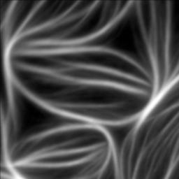
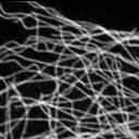
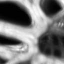
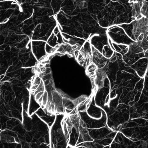
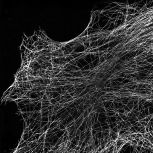
Figure 1: Images used for experiments

Table 1: Comparison of MAE at various execution times; PD: primal-dual splitting method [20]; PNw: proposed method with damped-Newton inner iteration; PMM: proposed method with MM based inner iteration.

Im	$\sigma$	Final (all)	PNw (200s)	PMM (200s)	PD (200s)	PNw (100s)	PMM (100s)	PD (100s)
1	3	0.598	0.609	0.610	1.114	0.624	0.668	1.961
	4	0.681	0.702	0.735	0.681	0.819	1.167	0.687
2	2.5	1.759	1.760	1.759	3.307	1.760	1.761	4.148
	4	1.990	1.990	1.991	1.990	1.991	1.990	1.998
3	3	0.959	0.959	0.959	8.820	0.979	0.965	10.762
	4	1.029	1.029	1.031	1.029	1.031	1.050	1.029
4	1	0.308	0.308	0.308	1.0432	0.311	0.311	1.0432
	2	0.351	0.354	0.362	0.352	0.360	0.377	0.359
5	2	0.551	0.551	0.559	0.609	0.554	0.566	0.749
	2.5	0.971	0.971	0.981	1.876	0.977	0.987	2.172
6	2.5	1.642	1.646	1.653	4.451	1.665	1.685	4.502
	3	1.694	1.699	1.710	2.485	1.718	1.768	3.078

Table 2: Comparison of MAE at various execution times; PD: primal-dual splitting method for different input scales ; PNw: proposed method with damped-Newton inner iteration; PMM: proposed method with MM based inner iteration.

	scale($\alpha^{\prime}$)	Final-all	PNw (200s)	PMM (200s)	PD (200s)	PNw (100s)	PMM (100s)	PD (100s)
Im1	0.75	0.503	0.511	0.514	0.716	0.553	0.551	1.456
	2	0.915	0.951	0.943	11.331	1.208	1.229	11.506
Im3	0.75	1.202	1.226	1.2205	1.1932	1.268	1.270	1.189
	2	3.560	3.590	3.599	8.929	3.654	3.668	9.504
Im6	0.75	0.853	0.853	0.854	4.158	0.865	0.863	5.800
	2	1.643	1.647	1.647	27.66	1.938	2.002	27.64

Table 3: Comparison of MAE at various execution times; PD: primal-dual splitting method for Hessian-Schatten norm ; PNw: proposed method with damped-Newton inner iteration; PMM: proposed method with MM based inner iteration.

Im	$\sigma$	Final (all)	PNw (200s)	PMM (200s)	PD (200s)	PNw (100s)	PMM (100s)	PD (100s)
1	3	0.595	0.613	0.610	1.882	0.686	0.689	2.777
	4	0.683	.703	0.704	0.686	0.801	0.772	0.739
2	2.5	1.651	1.653	1.652	4.143	1.655	1.654	4.932
	4	1.857	1.857	1.858	1.857	1.866	1.867	1.857
3	3	0.958	0.956	0.955	11.384	0.962	0.970	11.486
	4	1.028	1.032	1.032	1.027	1.047	1.128	1.349
4	1	0.306	0.308	0.308	1.0432	0.313	0.312	1.0432
	2	0.348	0.353	0.356	0.350	0.368	0.370	0.354
5	2	0.543	0.548	0.550	0.578	0.560	0.607	0.836
	2.5	0.917	0.922	0.920	1.073	0.932	0.928	1.105
6	2.5	1.649	1.665	1.667	5.019	1.701	1.725	5.135
	3	1.698	1.722	1.732	2.568	1.762	1.828	3.322

Table 4: Number of gradient computations from experiment set 1.

Im	$\sigma$	Target MAE	PNw	PMM	PD
1	3	1	52	154	3940
1	4	1	74	261	500
3	4	1.5	183	480	2235
5	2	1	4	15	2250
6	3	2	34	112	5060

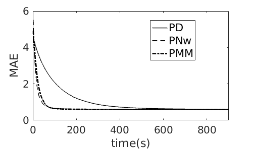
Figure 2: Evolution of of the result w.r.t. time for Im 1 with $\sigma=3$

Figure 3: Partially restored Images for Im 1 $\sigma=3$ (TV)

(a)Noisy (b)PNw (c) PMM (d)PD

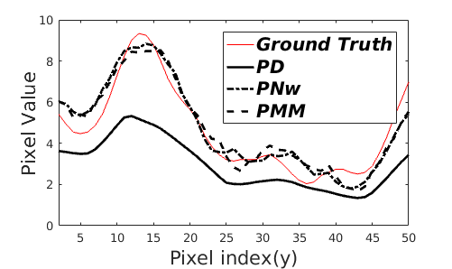
Figure 4: Scan lines for Im 1 $\sigma=3$ for section 4

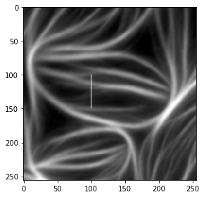
Figure 5: Cross-section (vertical line) for scan lines in fig. 4

In the third set of experiments, the test case of first set of experiment were rerun with TV-2 regularization replaced by Hessian-Schatten regularization with $q=1$ (see eq. 4). The results are given in the table 3. Here too, the relative performances of different methods in terms of convergence speed, confer to the same pattern as that of the first set of experiments. However, the actual MAEs attained by the methods are lower here, because Hessian-Schatten norm with $q=1$ has superior structure-preserving ability. As a special case, we observe MAEs obtained by the PD method from data set simulated from Im 4 with $\sigma=1$ obtained at 100s and 200s are identical. This Means that PD method is converging very slowly because of high value of Lipschitz constant. Next, the time-snap shots of partial results of various optimization methods applied on noisy-blurred image obtained from Im2 with $\sigma=2.5$ at 100s are given in the section 4. It is clear from the displayed images that results of proposed methods are visually better than the PD method. Further, similar to the first experiment set, the primal-dual splitting algorithm is more sensitive to change in $\sigma$.

In table 4, we show the number of gradient evaluations for the specified Target MAE corresponding to various test cases from the experiment set 1. Although, we have shown the comparisons only for specific test cases, we observed similar patterns for the entire data-set. These results show that primal-dual splitting method requires much more gradient evaluations which are expensive in this problem. The results from the sets of experiments confirm that the speed of primal-dual splitting method is sensitive to $\sigma$, and the maximum value of the pixels in blurred noisy image; this is because the upper bound on step size is the inverse of the Lipschitz constant of the gradient of data likelihood, which is proportional to $(1-e^{\frac{-1}{\sigma^{2}}})\exp(\frac{2\max_{i}(\boldsymbol{y}_{i})-1}{\sigma^{2}})$ [20]. This limitation is clearly not present in the proposed methods. Hence, the proposed algorithm has a wider applicability.

Figure 6: Partially restored Images for Im2 $\sigma=2.5$ at 100s (Hessian Schatten)

(a)Noisy (b)PNw (c) PMM (d)PD

5 Conclusions

We developed an ADMM based computational method for image restoration under mixed Poisson-Gaussian (PG) noise using convex non-differentiable regularization functionals. The main challenge was that there are no known methods for computing the proximal solution of PG log-likelihood functional, which is required for adopting ADMM approach for this problem. We developed iterative methods for computing the proximal solution of the PG log-likelihood functional along with the derivation of convergence proof. We also derived termination conditions for these iterative methods to be met for using them inside the ADMM iterative loop. This led to the first ADMM based method for image restoration under PG noise model using convex non-differentiable regularization functional. As in other image restoration problems, here too we demonstrated that the ADMM based method is faster than primal-dual splitting method. It should be emphasized that the approach used for the proofs of convergence are general, and hence the proposed method can be extended to any other complex likelihood models provided that the model has an uniform approximation for the gradient.

Appendix A: Proximal solutions for ADMM step

Since, some of the minimizations involved in the above iterative procedure can be solved exactly and yield a closed form solution, we first explain these exact minimizations involved in the procedure. In the ADMM scheme given in the equations (20)-(23), the quadratic minimization problem given in the Step 1 (equations (20) and (24)) can obviously be solved exactly, because equating the gradient of $Q(\cdot)$ gives a linear system of equations, whose solution can be expressed as follows:

$$\boldsymbol{g}^{(k+1)} =(\boldsymbol{I}+\boldsymbol{D^{T}D}+\boldsymbol{H^{T}H})^{-1}$$ (91)

$$\medmath{\left[\boldsymbol{b}^{(k)}+\frac{1}{\beta}\hat{\boldsymbol{b}}^{(k)}+\boldsymbol{D^{T}}(\boldsymbol{d}^{(k)}+\frac{1}{\beta}\hat{\boldsymbol{d}}^{(k)})\right.+\left.\boldsymbol{H^{T}(m}^{(k)}+\frac{1}{\beta}\hat{\boldsymbol{m}}^{(k)})\right].}$$ (92)

As all matrices involved in the above computation are block circulant with circulant blocks (corresponding to 2-D circular convolution), the matrix inversion involved in the above step can be efficiently computed using FFTs. Similarly, efficient inversions can be done using DCT and DST for symmetric and anti-symmetric boundary conditions respectively [31]. Note that, even if the matrices involved are not block circulant, the above inversion can be performed iteratively and still the convergence holds as the framework of Eckstein et al. [24] allows both the proximal operators to be inexact. Next, consider the subproblem corresponding to Step 3 (equation (22)). Although the sub-function is non-quadratic and non-differentiable, solving the problem exactly is possible thanks to the specific structure of the sub-function. The solution is the well-known multidimensional shrinkage operation ([32], eq. 3.24). For the reader’s convenience, we express the solution for our notations. We first note that, as far as the minimization with respect to $\boldsymbol{d}$ is concerned, $L_{\scriptscriptstyle D}({\bf g}^{(k+1)},\boldsymbol{d},\hat{\boldsymbol{d}}^{(k)})$ in the equation (10) can be replaced by the following function, which differs from $L_{\scriptscriptstyle D}({\bf g}^{(k+1)},\boldsymbol{d},\hat{\boldsymbol{d}}^{(k)})$ only by a constant that is independent of $\boldsymbol{d}$:

$$\begin{split}{L}_{\scriptscriptstyle D,k}(\boldsymbol{d})=&\medmath{\lambda F_{\scriptscriptstyle D}(\boldsymbol{d})+\frac{\beta}{2}\left\|\boldsymbol{d}-\bar{\boldsymbol{d}}^{(k+1)}\right\|^{2}_{2}};\medmath{\bar{\boldsymbol{d}}^{(k+1)}=\boldsymbol{D}{\bf g}^{(k+1)}-\frac{1}{\beta}\hat{\boldsymbol{d}}^{(k)}}\end{split}$$ (93)

Hence the minimization problem (22) can be expressed using the equation (93) as

$$\boldsymbol{d}^{(k+1)}=\operatorname*{arg\,min}_{\boldsymbol{d}}\lambda\sum_{i=1}^{N}\left\|\mathcal{E}(\boldsymbol{P}_{i}^{T}\boldsymbol{d})\right\|_{q}+\frac{\beta}{2}\left\|\boldsymbol{d}-\bar{\boldsymbol{d}}^{(k+1)}\right\|^{2}_{2}.$$

Let ${\cal S}([v_{1},v_{2},v_{3}]^{T})=\left[\begin{array}[]{cc}v_{1}&v_{3}\\ v_{3}&v_{2}\end{array}\right]$. Then the solution to the above problem can be written as

$$\mathbf{d}^{(k+1)}=\sum_{i}^{N^{2}}\mathbf{P}_{i}{\cal H_{T}}(\mathbf{P}_{i}^{T}\bar{\mathbf{d}}^{(k+1)},\lambda/\beta,q),$$

where

$${\cal H_{T}}(\mathbf{x},t,q)=\begin{cases}max(\|{\cal S}(\mathbf{x})\|_{F}-t,0)\frac{\mathbf{x}}{\|\cal{S}(\mathbf{x})\|_{F}},\;\mbox{for}\;\;q=2\\ {\cal S}^{-1}(|||{\cal S}(\mathbf{x})|||_{t}),\;\;\mbox{for}\;\;q=1,\end{cases}$$

with $|||\cdot|||_{t}$ denoting the operator that applies soft-thresholding on the Eigen values of its matrix argument and returns the resulting matrix.

Next, we consider the subproblem of the Step 4. Here too, as far as the minimization with respect to $\boldsymbol{b}$ is concerned, $L_{\scriptscriptstyle B}({\bf g}^{(k+1)},\boldsymbol{b},\hat{\boldsymbol{b}}^{(k)})$ in the equation (11) can be replaced by the following function, which differs from $L_{\scriptscriptstyle B}({\bf g}^{(k+1)},\boldsymbol{b},\hat{\boldsymbol{b}}^{(k)})$ only by a constant that is independent of $\boldsymbol{b}$:

$$\begin{split}{L}_{\scriptscriptstyle B,k}(\boldsymbol{b})=&F_{\scriptscriptstyle B}(\boldsymbol{b})+\frac{\beta}{2}\left\|\boldsymbol{b}-\bar{\boldsymbol{b}}^{(k+1)}\right\|^{2}_{2};\bar{\boldsymbol{b}}^{(k+1)}={\bf g}^{(k+1)}-\frac{1}{\beta}\hat{\boldsymbol{b}}^{(k)}\end{split}$$ (96)

Hence step 4 can be expressed as $\boldsymbol{b}^{(k+1)}=\operatorname*{arg\,min}_{\boldsymbol{b}}F_{\scriptscriptstyle B}(\boldsymbol{b})+\frac{\beta}{2}\left\|\boldsymbol{b}-\bar{\boldsymbol{b}}^{(k+1)}\right\|^{2}_{2}.$ The solution to the above problem can be expressed as [12]

$$\boldsymbol{b}^{(k+1)}={\cal P}_{[0,u^{\prime}]}(\bar{\boldsymbol{b}}^{(k+1)})$$

where ${\cal P}_{[0,u^{\prime}]}(\cdot)$ is the projection of its argument into the set bounded by the interval $[0,u^{\prime}]$. This projection is essentially clipping with the interval $[0,u^{\prime}]$.

Appendix B: Proof of propositions

Proof of Proposition 3.1.2 : Since the data fitting cost is separable across pixel indices, we replace $\boldsymbol{m}$ and $\boldsymbol{\bar{m}}$ by ${m}$ and $\bar{m}$ to denote a chosen pixel. Since, $\boldsymbol{\gamma}_{1}({m},{m}^{\prime})$ is the gradient of $F_{\scriptscriptstyle{M}}({m},{m^{\prime}})$, it satisfies the inequality that any sub-gradient should satisfy since the function is convex. Next, since $\bar{F}_{\scriptscriptstyle{M}}({m},{m^{\prime}})$ is $\infty$ when $m$ goes out of bounds, $\boldsymbol{\gamma}_{1}({m},{m}^{\prime})$ should also satisfy the sub-gradient inequality for $\bar{F}_{\scriptscriptstyle{M}}({m},{m^{\prime}})$ for $m\in[l,u]$. This means that $\boldsymbol{\gamma}_{1}({m},{m}^{\prime})+\beta(m-\bar{m})$ is a sub-gradient for $L_{M,k}(m,m^{\prime})$ for $m\in[l,u]$. Now if we show that $\boldsymbol{\gamma}_{1,\Delta}({m},{m}^{\prime})$ is $\epsilon$-sub-gradient of $F_{M}(m,m^{\prime})$, $\boldsymbol{\gamma}_{1,\Delta}({m},{m}^{\prime})+\beta(m-m^{\prime})$ will be clearly be the $\epsilon$-sub-gradient of $L_{M,k}(m,m^{\prime})$ for $m\in[l,u]$ because of the same set of arguments used above. To this end, we first note that ${F}_{\scriptscriptstyle M}(m_{1},m^{\prime})\geq{F}_{\scriptscriptstyle M}(m,m^{\prime})+\gamma_{1}(m,m^{\prime})(m_{1}-m)$. This can be written as ${F}_{\scriptscriptstyle M}(m_{1},m^{\prime})\geq{F}_{\scriptscriptstyle M}(m,m^{\prime})+\gamma_{1,\Delta}(m,m^{\prime})(m_{1}-m)+(\gamma_{1}(m,m^{\prime})-\gamma_{1,\Delta}(m,m^{\prime}))(m_{1}-m)$. Next we show below that $|\gamma_{1}(m,m^{\prime})-\gamma_{1,\Delta}(m,m^{\prime})|\leq\bar{B}(1-erf(\frac{\Delta}{\sqrt{2}}))$ where $\bar{B}$ is a constant and $erf$ is error function [33]. Since $erf(\frac{\Delta}{\sqrt{2}})\rightarrow 1$ as $\Delta\rightarrow\infty$, we have that ${F}_{\scriptscriptstyle M}(m_{1},m^{\prime})\geq{F}_{\scriptscriptstyle M}(m,y)+\gamma_{1,\Delta}(m,m^{\prime})(m_{1}-m)-\epsilon$, where $\epsilon=\bar{B}(1-erf(\frac{\Delta}{\sqrt{2}}))(u-l)$ is real number that goes to zero as $\Delta\rightarrow\infty$. This means that $\boldsymbol{\gamma}_{1,\Delta}({m},{m}^{\prime})$ is an $\epsilon$-sub-gradient of $F_{M}(m,m^{\prime})$.

To show that $|\gamma_{1,\Delta}(m,m^{\prime})-\gamma_{1}(m,m^{\prime})|\leq\bar{B}(1-erf(\frac{\Delta}{\sqrt{2}}))$ where $\bar{B}$ is a constant: From the equations eq. 31 and eq. 35, we can deduce that $|\gamma_{1,\Delta}(m,m^{\prime})-\gamma_{1}(m,m^{\prime})|=\frac{|s(m,m^{\prime}-1)s_{\Delta}(m,m^{\prime})-s_{\Delta}(m,m^{\prime}-1)s(m,m^{\prime})|}{s(m,m^{\prime})s_{\Delta}(m,m^{\prime})}.$ Next, from expressions (32) and (34), we find that both $s(m,m^{\prime})$ and $s_{\Delta}(m,m^{\prime})$ are lower bounded by $\exp(-\frac{(m^{\prime})^{2}}{2\sigma^{2}})$. Letting $B=\exp(\frac{(m^{\prime})^{2}}{\sigma^{2}})$ gives $|\gamma_{1,\Delta}(m,m^{\prime})-\gamma_{1}(m,m^{\prime})|\leq B|s(m,m^{\prime}-1)s_{\Delta}(m,m^{\prime})-s_{\Delta}(m,m^{\prime}-1)s(m,m^{\prime})|.$ Adding and subtracting $s(m,m^{\prime})s(m,m^{\prime}-1)$ gives

$$|\gamma_{1,\Delta}(m,m^{\prime})-\gamma_{1}(m,m^{\prime})|\leq$$ (97)

$$B\Big{[}s(m,m^{\prime}-1)\bar{s}_{\Delta}(m,m^{\prime})+s(m,m^{\prime})\bar{s}_{\Delta}(m,m^{\prime}-1)\Big{]},$$

where $\bar{s}_{\Delta}(m,m^{\prime})=|s(m,m^{\prime})-s_{\Delta}(m,m^{\prime})|.$ Chouzenoux et al. [20] have shown that $\bar{s}_{\Delta}(m,m^{\prime})\leq\sqrt{2\pi}\sigma\frac{m^{n^{*}}}{n^{*}!}\exp(\frac{-(m^{\prime}-\alpha n^{*})^{2}}{2\sigma^{2}})(1-erf(\frac{\Delta}{\sqrt{2}}))$ for some $n^{*}\in\mathbb{N}$. Further note that, $\frac{m^{n^{*}}}{n^{*}!}\exp(\frac{-(m^{\prime}-\alpha n^{*})^{2}}{2\sigma^{2}})\leq s(m,m^{\prime})$. Moreover, note that $s(m,m^{\prime})\leq\sum_{n=0}^{\infty}\frac{m^{n}}{n!}=e^{m}\leq e^{u}$, where $u$ is upper bound on $m$. Putting all these things together, gives the required result.

Proof of Proposition 3.1.2: Here too, since the data fitting cost is separable across pixel indices, we replace $\boldsymbol{m}$ and $\boldsymbol{m}^{\prime}$ by ${m}$ and ${m}^{\prime}$ to denote a chosen pixel. We have to show the following sub-gradient inequality for all $m$ in $[l,u]$ and $m_{1}\in\mathbb{R}$: $L_{M,k}(m_{1},m^{\prime})\geq L_{M,k}(m,m^{\prime})+\eta(m,m^{\prime})(m_{1}-m).$ Since, $L_{M,k}(m_{1},m^{\prime})$ is $\infty$ for $m_{1}\notin[l,u]$, and ${\eta}({m},{m}^{\prime})$ is identical to $\zeta(m,m^{\prime})$ for $m\in(l,u)$, it only remains to show that ${\eta}({m},{m}^{\prime})$ satisfies the above equation for $m$ in $\{l,u\}$ and $m_{1}\in[l,u]$. Now for $m=l$, ${\eta}({m},{m}^{\prime})$ is a projection of $\zeta(m,m^{\prime})$ onto non-positive real line, and hence, ${\zeta}({m},{m}^{\prime})\geq{\eta}({m},{m}^{\prime})$. Since $(m_{1}-l)$ positive, we have ${\zeta}({m},{m}^{\prime})(m_{1}-m)\geq{\eta}({m},{m}^{\prime})(m_{1}-m)$ for $m=l$. In a similar way, we can show that the above inequality is satisfied for $m=u$ also. This means that the sub-gradient inequality is satisfied for $m$ in $\{l,u\}$ and $m_{1}\in[l,u]$.

It remains to be proven that $\eta(m,m^{\prime})\rightarrow 0$ at minimum of $L_{M,k}$. Note that finding minimum of $L_{M,k}$ is equivalent to finding the minimum of $L_{M,k}^{\prime}(m,m^{\prime})=F_{M}(m,m^{\prime})+(\beta/2)(m-\bar{m})^{2}$ subject to $m\in\Omega=[l,u]$. The first order necessary condition for the general case is that the inner product between any feasible direction of the constraint set $\Omega$ [12] and the gradient should be non-negative. In our problem, for $m\in(l,u)$, the feasible directions are both positive and negative real axes, and hence, the first order condition means that $\zeta(m,m^{\prime})=0$. Next, for $m=l$, the feasible direction is positive real axis, and hence, the first order condition means that projection of $\zeta(m,m^{\prime})$ onto non-positive real axis should be zero. Further, for $m=u$, the feasible direction is negative real axis, and hence, the first order condition means that projection of $\zeta(m,m^{\prime})$ onto non-negative real axis should be zero. The above three statements imply that $\eta(m,m^{\prime})$ should be zero.

Since, any projection is non expansive operator, we have the following: $|\gamma_{1}(m,m^{\prime})-\gamma_{1,\Delta}(m,m^{\prime})|\rightarrow 0$ as $\Delta\rightarrow\infty$, implies that $|\eta(m,m^{\prime})-\eta_{\Delta}(m,m^{\prime})|\rightarrow 0$ as $\Delta\rightarrow\infty$. Hence $\eta_{\Delta}(m,m^{\prime})\rightarrow 0$ as $\Delta\rightarrow\infty$ at the minimum point.

Proof of Proposition 3.2.1: We use the following theorem to prove the proposition. Consider iteration $x^{(l+1)}=P_{X,D_{l}^{-1}}(x^{(l)}-\alpha^{(l+1)}D_{l}u^{(l)})$ for solving the problem $\operatorname*{arg\,min}_{\boldsymbol{x}\in X}f(\boldsymbol{x})$.

Here, the scaled projection is defined as $P_{X,F}(\boldsymbol{g}):=\operatorname*{arg\,min}_{x\in X}(\boldsymbol{(x-g)}^{T}F(\boldsymbol{(x-g)}))$ where $F$ is a positive definite matrix with bounded eigen values. $\boldsymbol{u}^{(l)}$ is an $\epsilon_{l}$ sub-gradient of the $f$ at $\boldsymbol{x}^{(l)}$ i.e. $\boldsymbol{u}^{(l)}\in\partial_{\epsilon_{l}}f(\boldsymbol{x}^{(l)})$ and $D_{l}$ is a gradient scaling matrix(symmetric positive definite with bounded eigen values).

Theorem 1

(Bonettini et al., [29]) Let ${x^{(l)}}\in\Omega$ be the sequence generated by the above iteration , for a given sequence $\{\epsilon_{l}\}\subset R$, $\epsilon_{l}\geq 0$. Assume that the set of the solutions of the above minimization problem $X^{*}$ is non-empty and that there exists a positive constant $\rho$ such that $\|\boldsymbol{u}^{(l)}\|\leq\rho$ and a sequence of positive numbers ${L_{l}}$ such that $\|D_{l}\|\leq L_{l},\|{D_{l}}^{-1}\|\leq L_{l}$, with $1\leq L_{l}\leq L$ for some positive constant $L$, for all $l\geq 0$. If the following conditions holds, then the sequence generated by the iterations converge to a point in $X^{*}$ (1) $\epsilon_{l}\rightarrow 0$ (2) $\sum\limits_{l=0}^{\infty}\alpha^{(l)}=\infty$ (3) $\sum\limits_{l=0}^{\infty}(\alpha^{(l)})^{2}<\infty$ (4) $\sum\limits_{l=0}^{\infty}\alpha^{(l)}\epsilon_{l}<\infty$ (5) $L_{l}^{2}=1+\gamma_{l}$,$\sum\limits_{l=0}^{\infty}\gamma_{l}<\infty$

In our case, the iterations proposed are,

$$\boldsymbol{m}_{l+1}^{(k)}=$$ (98)

$$\medmath{{{\cal P}}_{{[l,u]}}\left({m}_{l}^{(k)}-\alpha_{l}\left[{\zeta}_{1,\Delta_{l}}({m}_{l}^{(k)},{m}^{\prime})\right]/\left[{{\Gamma_{l}}\left({\gamma}_{2,\triangle_{l}}({m}_{l}^{(k)},{m}^{\prime})+\beta\right)}\right]\right)}$$ (99)

Since, our set $X$ is $[m,M]$, simply one dimension interval, scaled projection is same as simple projection. Also our scaling factor is obtained after the projection on set$[\frac{1}{\sqrt{\delta_{l}}},\sqrt{\delta_{l}}]$ and $\delta_{l}$ which plays the role of $L_{l}^{2}$ is chosen to be $\delta_{l}=1+\frac{C_{2}}{(l+1)^{2}}$, because of this scaling factor is bounded between $1$ and $\sqrt{1+C_{2}}$. It has been proved previously in this paper that $\zeta_{\Delta_{l}}(m,m^{\prime})$ is an $\epsilon$ Sub-gradient of $L_{M,k}(m,m^{\prime},\bar{m})$ i.e. $\zeta_{\Delta_{l}}(m,m^{\prime})\in$ $\partial_{\epsilon}{F_{M}(m,m^{\prime})}$ where $\epsilon=\bar{B}(1-erf(\frac{\Delta}{\sqrt{2}}))|u-l|$. Clearly, the $\epsilon$-sub-gradient is upper-bounded. Since $\Delta$ is the term that determines the number of terms in summation, for convergence we increase $\Delta_{l}$ in as iteration number increases by the following rule: $\Delta_{l}=[C_{\Delta}l+1]$ (where $C_{\Delta}$ is any positive constant, $[x]$ denotes the greatest integer less than x). Now since, $\Delta_{l}\rightarrow\infty\implies\bar{B}(1-erf(\frac{\Delta}{\sqrt{2}}))|u-l|\rightarrow 0$ as $erf(\frac{\Delta}{\sqrt{2}})\rightarrow 1$. This justifies satisfiability of condition (1) of the theorem. Since, $\alpha^{(l)}$ is chosen as $\alpha^{(l)}=\frac{C}{l+1}$, conditions (2) and (3) are satisfies as it is a well known square summable sequence but not summable. On substituting $\Delta_{l}=[C_{\Delta}l+1]$, we get $\epsilon_{l}=\bar{B}(1-erf(\frac{[C_{\Delta}l+1]}{\sqrt{2}}))|l-u|$
Since, $1-erf(z)<\frac{exp(-z^{2})}{\sqrt{\pi}z}$ [33]$\implies\epsilon_{l}<\sqrt{2}\bar{B}(\frac{\exp(-.5{[C_{\Delta}l+1]}^{2})}{\sqrt{\pi}[C_{\Delta}l+1]})|u-l|$ Using $(\exp(-.5[C_{\Delta}l+1]^{2}))<1$ and substituting for $\alpha^{(l)}$, we get, $\sum\limits_{l=0}^{\infty}\alpha_{l}\epsilon_{l}<\alpha_{0}\epsilon_{0}+\sum\limits_{l=1}^{\infty}\sqrt{2}\bar{B}\frac{C}{\sqrt{\pi}C_{\Delta}l(l+1)})|l-u|<\infty$. This satisfies condition (4).

On comparing with our set of iterations $\delta_{l}=1+\frac{C_{2}}{(l+1)^{2}}$ plays the role of $L_{l}^{2}$, therefore $\gamma_{l}$ for our case becomes, $\frac{C_{2}}{(l+1)^{2}}$ which is a hummable sequence, and hence this satisfies condition (5)

Proof of Proposition 3.2.2: From equation (44), we get $f_{\scriptscriptstyle P,M^{\prime}|m}({p},{m^{\prime}}|m)=\frac{m^{p}}{\sqrt{2\pi}\sigma{p}!}\exp(-(\frac{\boldsymbol{m^{\prime}}-\alpha{p}}{\sqrt{2}\sigma})^{2}-(m)).$ Applying log gives taking the required expectation, we get $G_{M}(m,m^{\prime},m_{l})=\mathcal{E}_{\scriptscriptstyle{P}|{M^{\prime}},m_{l}}\{\ln f_{\scriptscriptstyle P,M^{\prime}|m}({p},{m^{\prime}}|m)\}$ $=\ln(m)\mathcal{E}_{{P}|{M^{\prime}},m_{l}}({p})-m+cons,$ where $\mathcal{E}_{\scriptscriptstyle{P}|\boldsymbol{M^{\prime}},m_{l}}({p})=\sum_{\boldsymbol{p}=0}^{\infty}{p}f_{P|M^{\prime},m}({p}|{y},m_{l})$. Then the minimization given in the equation (42) is equivalent to solving the following equation: $\frac{dG_{M}(m,m^{\prime},m_{l})}{dm}+\beta({m}-\bar{m})=0\Longrightarrow\frac{{q}}{m_{(l+1)}}-1-\beta({(m)_{(l+1)}}+{\bar{m}})=0$. Solving this equation gives required expression.

Proof of Proposition 3.3: We have $|\eta_{\Delta}(m,m^{\prime})-{\eta{(m,m^{\prime})}}|\leq|\gamma_{1}(m,m^{\prime})-\gamma_{1,\Delta}(m,m^{\prime})|\leq\bar{B}(1-erf(\frac{\Delta}{\sqrt{2}}))$, the above inequation follows from section showing Proof of proposition 1. So, instead of condition (1), • ‣ 2.3, a verifiable condition that can be checked is $|\eta_{\Delta_{l}}(m_{l},m^{\prime})|+\bar{B}(1-erf(\frac{\Delta_{l}}{\sqrt{2}}))<\theta_{k}$

Following the above approach a similar condition to remedy the inexactness in the gradient can be derived for condition (2). It can be observed that $\boldsymbol{w}^{(k)}=\boldsymbol{w}^{(0)}-\beta\sum_{i=0}^{k-1}\eta(\boldsymbol{{m}^{(i)}},\boldsymbol{m^{\prime}})$. $\boldsymbol{w}^{(0)}$ can be chosen to be zero vector without disturbing the criteria. Now, to derive a sufficient condition to obtain an upperbound on $2|\langle\boldsymbol{w}^{(k)}-\boldsymbol{m}^{(k)}_{l},{\eta(\boldsymbol{m}^{(k)}_{l},\boldsymbol{m^{\prime}})}\rangle|+\|{\eta(\boldsymbol{m}^{(k)}_{l},\boldsymbol{m^{\prime}})}\|^{2}$ $=2|\langle{-\beta\sum_{i=0}^{k-1}\eta(\boldsymbol{m}^{(i)},\boldsymbol{m^{\prime}})-\boldsymbol{m}^{(k)}_{l},{\eta(\boldsymbol{m}^{(k)}_{l},\boldsymbol{m^{\prime}})}\rangle}|+\|{\eta(\boldsymbol{m}^{(k)}_{l},\boldsymbol{m}^{\prime})}\|^{2}$. Now, we do not have the exact value of the $\eta(\cdot)$ but we have a $\Delta$ approximation which is based on $\Delta$ gradient approximation. Letting $\eta(\boldsymbol{m}^{(k)}_{l},\boldsymbol{m^{\prime}})=\eta_{\Delta_{l}}({\boldsymbol{m^{(l)}}},\boldsymbol{m^{\prime}})+e_{l}$ where $e_{l}$ is the approximation error, gives $\leq 2|\langle{\beta\sum_{i=0}^{k-1}\eta_{\Delta_{i}}({\boldsymbol{m}^{(i)},\boldsymbol{m^{\prime}}})+e_{i}+\boldsymbol{m}^{(k)}_{l},{\eta(\boldsymbol{m}^{(k)}_{l},\boldsymbol{m^{\prime}})}}\rangle|+\|{\eta(\boldsymbol{m}^{(k)}_{l},\boldsymbol{m^{\prime}})}\|^{2}$ $\leq 2|\langle{\beta\sum_{i=0}^{k-1}\eta_{\Delta_{i}}({\boldsymbol{m}^{(i)},\boldsymbol{m^{\prime}}})+\boldsymbol{m}^{(k)}_{l},\eta({\boldsymbol{m}^{(i)},\boldsymbol{m^{\prime}}}})\rangle|+2\beta\sum_{i=0}^{k-1}|\langle e_{i},\eta({\boldsymbol{m}^{(i)},\boldsymbol{m^{\prime}}})\rangle|+\|\eta_{\Delta_{l}}({\boldsymbol{m}^{(k)}_{l},\boldsymbol{m^{\prime}}})+e_{l}\|^{2}$ (Using Triangle inequality). Now, substitute $\boldsymbol{w}_{\Delta}^{(k)}=-\beta\sum_{i=0}^{k-1}\eta_{\Delta_{i}}{(\boldsymbol{m}^{(i)},\boldsymbol{m^{\prime}})}$ and use cauchy Schwartz Inequality to get

$$=2|\langle\boldsymbol{w}_{\Delta}^{(k)}-\boldsymbol{m}^{(k)}_{l},{\eta_{\Delta_{l}}(\boldsymbol{m}^{(k)}_{l},\boldsymbol{m^{\prime}})}+e_{l}\rangle|+$$

$$2\beta\sum_{i=0}^{k-1}|\langle e_{i},\eta_{\Delta_{l}}{(\boldsymbol{m}^{(k)}_{l},\boldsymbol{m^{\prime}})}+e_{l}\rangle|+\|{\eta_{\Delta_{l}}(\boldsymbol{m}^{(k)}_{l},\boldsymbol{m^{\prime}})}+e_{l}\|^{2}$$

$$\leq 2|\langle\boldsymbol{w}_{\Delta}^{(k)}-\boldsymbol{m}^{(k)}_{l},{\eta_{\Delta_{l}}(\boldsymbol{m}^{(k)}_{l},\boldsymbol{m^{\prime}})}\rangle|$$

$$+2\|\boldsymbol{w}_{\Delta}^{(k)}-\boldsymbol{m}^{(k)}_{l}\|\ \|{e_{l}}\|+(\|\eta_{\Delta_{l}}{(\boldsymbol{m}^{(k)}_{l},\boldsymbol{m^{\prime}})}\|+\|e_{l}\|$$

$$+2\beta\sum_{i=0}^{k-1}\|e_{i}\|)\ (\|\eta_{\Delta_{l}}{(\boldsymbol{m}^{(k)}_{l},\boldsymbol{m}^{\prime})}\|+\|e_{l}\|)$$

$=2|\langle\boldsymbol{w}_{\Delta}^{(k)}-\boldsymbol{m}^{(k)}_{l},{\boldsymbol{\eta}_{l,\Delta_{l}}^{(k)}}\rangle|+(\|\boldsymbol{\eta}_{l,\Delta_{l}}^{(k)}\|+\|e_{l}\|)^{2}+Z_{l}(w_{\Delta_{l}}^{(k)},\boldsymbol{\eta}_{l,\Delta_{l}}^{(k)})$, where $Z_{l}=2\|\boldsymbol{w}_{\Delta}^{(k)}-\boldsymbol{m}^{(k)}_{l}\|\ \|{e_{l}}\|+(2\beta\sum_{i=0}^{k-1}\|e_{i}\|)\ (\|\eta_{\Delta_{l}}{(\boldsymbol{m}^{(k)}_{l},\boldsymbol{m}^{\prime})}\|+\|e_{l}\|)$. Upperbound on each $\|e_{j}\|$ can be obtained from as $\|e_{j}\|\leq\sqrt{N}\bar{B}(1-erf(\frac{\Delta_{j}}{\sqrt{2}}))$ where N is the number of pixels in the image. The above expression can be used to verify the required condition.

References

- [1] A. Jezierska, C. Chaux, J.-C. Pesquet, H. Talbot, and G. Engler, “An em approach for time-variant poisson-gaussian model parameter estimation,” IEEE Transactions on Signal Processing, vol. 62, no. 1, pp. 17–30, 2014.
- [2] L. Zhu, W. Zhang, D. Elnatan, and B. Huang, “Faster storm using compressed sensing,” Nature methods, vol. 9, no. 7, p. 721, 2012.
- [3] Y. Marnissi, Y. Zheng, and J.-C. Pesquei, “Fast variational bayesian signal recovery in the presence of poisson-gaussian noise,” in Acoustics, Speech and Signal Processing (ICASSP), 2016 IEEE International Conference on. IEEE, 2016, pp. 3964–3968.
- [4] F. Benvenuto, A. La Camera, C. Theys, A. Ferrari, H. Lantéri, and M. Bertero, “The study of an iterative method for the reconstruction of images corrupted by poisson and gaussian noise,” Inverse Problems, vol. 24, no. 3, p. 035016, 2008.
- [5] D. L. Snyder, C. W. Helstrom, A. D. Lanterman, R. L. White, and M. Faisal, “Compensation for readout noise in ccd images,” JOSA A, vol. 12, no. 2, pp. 272–283, 1995.
- [6] M. A. Figueiredo and R. D. Nowak, “An em algorithm for wavelet-based image restoration,” IEEE Transactions on Image Processing, vol. 12, no. 8, pp. 906–916, 2003.
- [7] A. Chambolle, “An algorithm for total variation minimization and applications,” Journal of Mathematical imaging and vision, vol. 20, no. 1-2, pp. 89–97, 2004.
- [8] L. I. Rudin, S. Osher, and E. Fatemi, “Nonlinear total variation based noise removal algorithms,” Physica D: nonlinear phenomena, vol. 60, no. 1-4, pp. 259–268, 1992.
- [9] S. Lefkimmiatis, A. Bourquard, and M. Unser, “Hessian-based norm regularization for image restoration with biomedical applications,” IEEE Transactions on Image Processing, vol. 21, no. 3, pp. 983–995, 2012.
- [10] M. Lysaker and X.-C. Tai, “Iterative image restoration combining total variation minimization and a second-order functional,” International journal of computer vision, vol. 66, no. 1, pp. 5–18, 2006.
- [11] B. Bajić, J. Lindblad, and N. Sladoje, “Blind restoration of images degraded with mixed poisson-gaussian noise with application in transmission electron microscopy,” in Biomedical Imaging (ISBI), 2016 IEEE 13th International Symposium on. IEEE, 2016, pp. 123–127.
- [12] D. P. Bertsekas, Nonlinear programming. Athena scientific Belmont, 1999.
- [13] F. J. Anscombe, “The transformation of poisson, binomial and negative-binomial data,” Biometrika, vol. 35, no. 3/4, pp. 246–254, 1948.
- [14] B. Zhang, M. J. Fadili, J. . Starck, and J. . Olivo-Marin, “Multiscale variance-stabilizing transform for mixed-poisson-gaussian processes and its applications in bioimaging,” in 2007 IEEE International Conference on Image Processing, vol. 6, Sep. 2007, pp. VI – 233–VI – 236.
- [15] D. L. Donoho, “Nonlinear wavelet methods for recovery of signals, densities, and spectra from indirect and noisy data,” in In Proceedings of Symposia in Applied Mathematics. Citeseer, 1993.
- [16] A. Chakrabarti and T. Zickler, “Image restoration with signal-dependent camera noise,” arXiv preprint arXiv:1204.2994, 2012.
- [17] Y. Marnissi, Y. Zheng, E. Chouzenoux, and J.-C. Pesquet, “A variational bayesian approach for image restoration—application to image deblurring with poisson–gaussian noise,” IEEE Transactions on Computational Imaging, vol. 3, no. 4, pp. 722–737, 2017.
- [18] B. Zhang, M. Fadili, J.-L. Starck, and J.-C. Olivo-Marin, “Multiscale variance-stabilizing transform for mixed-poisson-gaussian processes and its applications in bioimaging,” in Image Processing, 2007. ICIP 2007. IEEE International Conference on, vol. 6. IEEE, 2007, pp. VI–233.
- [19] Q. Gao, S. Eck, J. Matthias, I. Chung, J. Engelhardt, K. Rippe, and K. Rohr, “Bayesian joint super-resolution, deconvolution, and denoising of images with poisson-gaussian noise,” in 2018 IEEE 15th International Symposium on Biomedical Imaging (ISBI 2018). IEEE, 2018, pp. 938–942.
- [20] E. Chouzenoux, A. Jezierska, J.-C. Pesquet, and H. Talbot, “A convex approach for image restoration with exact poisson–gaussian likelihood,” SIAM Journal on Imaging Sciences, vol. 8, no. 4, pp. 2662–2682, 2015.
- [21] J. Eckstein and D. P. Bertsekas, “On the douglas—rachford splitting method and the proximal point algorithm for maximal monotone operators,” Mathematical Programming, vol. 55, no. 1, pp. 293–318, 1992.
- [22] M. A. Figueiredo and J. M. Bioucas-Dias, “Restoration of poissonian images using alternating direction optimization,” IEEE transactions on Image Processing, vol. 19, no. 12, pp. 3133–3145, 2010.
- [23] M. V. Afonso, J. M. Bioucas-Dias, and M. A. Figueiredo, “Fast image recovery using variable splitting and constrained optimization,” IEEE transactions on image processing, vol. 19, no. 9, pp. 2345–2356, 2010.
- [24] J. Eckstein and W. Yao, “Approximate admm algorithms derived from lagrangian splitting,” Computational Optimization and Applications, vol. 68, no. 2, pp. 363–405, 2017.
- [25] M. Ghulyani and M. Arigovindan, “Fast total variation based image restoration under mixed poisson-gaussian noise model,” in 2018 IEEE 15th International Symposium on Biomedical Imaging (ISBI 2018), April 2018, pp. 1264–1267.
- [26] S. Lefkimmiatis, J. P. Ward, and M. Unser, “Hessian schatten-norm regularization for linear inverse problems,” IEEE Transactions on Image Processing, vol. 22, no. 5, pp. 1873–1888, May 2013.
- [27] M. V. Afonso, J. M. Bioucas-Dias, and M. A. Figueiredo, “An augmented lagrangian approach to the constrained optimization formulation of imaging inverse problems,” IEEE Transactions on Image Processing, vol. 20, no. 3, pp. 681–695, 2011.
- [28] S. Boyd and L. Vandenberghe, Convex optimization. Cambridge university press, 2004.
- [29] S. Bonettini, A. Benfenati, and V. Ruggiero, “Scaling techniques for epsilon-subgradient methods,” SIAM Journal on Optimization, vol. 26, no. 3, pp. 1741–1772, 2016.
- [30] C. J. Wu, “On the convergence properties of the em algorithm,” The Annals of statistics, pp. 95–103, 1983.
- [31] S. A. Martucci, “Symmetric convolution and the discrete sine and cosine transforms,” IEEE Transactions on Signal Processing, vol. 42, no. 5, pp. 1038–1051, 1994.
- [32] W.-S. Xie, Y.-F. Yang, and B. Zhou, “An admm algorithm for second-order tv-based mr image reconstruction,” Numerical Algorithms, vol. 67, no. 4, pp. 827–843, 2014.
- [33] F. R. Kschischang, “The Complementary Error Function,” 2017, uRL: http://www.comm.utoronto.ca/frank/notes/erfc.pdf. Last visited on 2018/30/04.