A Convex Optimization-based Dynamic Model Identification Package for the da Vinci Research Kit

Abstract

The da Vinci Research Kit (dVRK) is a teleoperated surgical robotic system. For dynamic simulations and model-based control, the dynamic model of the dVRK is required. We present an open-source dynamic model identification package for the dVRK, capable of modeling the parallelograms, springs, counterweight, and tendon couplings, which are inherent to the dVRK. A convex optimization-based method is used to identify the dynamic parameters of the dVRK subject to physical consistency. Experimental results show the effectiveness of the modeling and the robustness of the package. Although this software package is originally developed for the dVRK, it is feasible to apply it on other similar robots.

I Introduction

The da Vinci Research Kit (dVRK) is an open-source teleoperated surgical robotic system whose mechanical components are obtained from the first generation of the da Vinci Surgical Robot [1]. It has made research on surgical robotics more accessible. To date, researchers from over 30 institutes around the world are using the physical dVRK, and some others are using the dVRK simulations [1, 2, 3].

Model-based control has proven capable to increase the control precision and response speed of robotic arms [4], as well as their capability to deal with surrounding environment [5]. Although these techniques have already been widely used on traditional industrial robotic arms and collaborative robotic arms, their research on surgical robots can be rarely found due to the lack of accurate dynamic models. Moreover, several open-source simulators for the dVRK [2, 3] have been developed recently, which can potentially accelerate the development of robotic algorithms and surgical training. However, accurate dynamic model, which is essential for realistic simulation, is absent in all of these simulators.

Several studies have been reported regarding the dynamic model identification of the dVRK [6, 7, 8, 9]. [6] [6] identified the dynamic parameters of the Master Tool Manipulator (MTM) and Patient Side Manipulator (PSM) of the dVRK using the method proposed in [10]. In our previous work [8], we replicated the approach in [6] and identified the dynamic parameters related to the first three joints of the PSM. With the obtained dynamic parameters, we implemented a collaborative object manipulation based on impedance control, with one PSM manually controlled by a user and the other following the former one’s motion automatically. [7] [7] and [9] [9] identified the dynamic parameters of the PSM using Least-square Regression and used them for sensorless external force estimation for force feedback.

Despite a significant amount of work regarding the dynamic model identification of the dVRK manipulators, none of them can be used directly by other researchers since the dynamic parameters vary between different robots of the same make and model due to manufacturing and assembly variances. Furthermore, the assembly components of robots are subject to deformation and wear & tear along their life cycle, which can potentially alter the dynamic model. As such, dynamic model identification is required before the implementation of any robust model-based control algorithm. This requirement drives the need for a robust open-source dynamic model identification package.

There are existing software packages for the dynamic model identification of robotic manipulators, such as SymPybotics [11], FloBaRoID [12], and OpenSYMORO [13]. However, SymPybotics and FloBaRoID are targeting at generic open-chain manipulators and lack the capability of modeling parallelograms, springs, counterweights, and tendon couplings, which are inherent to the mechanical design of the dVRK. Although OpenSYMORO is able to model closed-chain mechanisms, no physical consistency (also called physical feasibility) [14] is considered in parameter identification, which can potentially lead to unexpected behavior in simulations and model-based control [15].

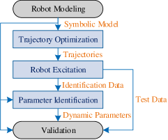
Figure 1: Workflow of dynamic model identification.

The physical consistency conditions enforce the positivity of kinetic energy [15] and the density realizability of a link [16] by constraining the inertia tensor to be positive definite and the sum of any two of its eigenvalues to be larger than the third one. These two conditions were formulated into semi-definite constraints with Linear Matrix Inequality (LMI) techniques in [10, 17, 14], enabling the use of convex optimization tools to solve the identification problem. Moreover, [17] [17] showed physical consistency constraints can improve identification performance by reducing overfitting.

The purpose of this work is to develop an open-source dynamic model identification package for the dVRK considering full physical consistency. Based on the workflow of dynamic model identification in Fig. 1, we structure this paper into seven sections. Sections II and III explain the mathematical formulation of the kinematic and dynamic modeling of the MTM and PSM. Section IV describes the trajectory optimization method to improve parameter identification quality. Section V presents the identification approach to obtain physically consistent dynamic parameters. The experimental results are presented to validate the proposed approaches in Section VI. The concluding arguments are entailed in Section VII.

II Kinematic Modeling of the dVRK

To build the relationship between the robot joint motion in the dVRK-ROS package [1] and the torque of each motor, several types of joint coordinates are defined. $\boldsymbol{q}^{d}$ are the joint coordinates used in the dVRK-ROS package. $\boldsymbol{q}=\begin{bmatrix}(\boldsymbol{q}^{b})^{\top}&\boldsymbol{(q}^{a})^{\top}\end{bmatrix}^{\top}$ are the joint coordinates used in the kinematic modeling in this work, where $\boldsymbol{q}^{b}$ are the basis joint coordinates which can adequately represent the kinematics of the robot, and $\boldsymbol{q}^{a}$ are the additional joint coordinates, which represent the other joint coordinates in the parallel mechanism and can be represented by the linear combination of $\boldsymbol{q}^{b}$. Since both the MTM and PSM have seven actuated degrees of freedom (DOF), the basis joint coordinates can be represented by $\boldsymbol{q}^{b}=\begin{bmatrix}q_{1}&q_{2}&\ldots&q_{7}\end{bmatrix}^{\top}$. $\boldsymbol{q}^{m}$ are the equivalent motor coordinates which are considered at joints, with the reduction ratio caused by gearboxes and tendons included for most motors unless explicitly specified. Finally, $\boldsymbol{q}^{c}=\begin{bmatrix}\boldsymbol{q}^{\top}&(\boldsymbol{q}^{m})^{\top}\end{bmatrix}^{\top}$ define the complete joint coordinates. The relation between these joint coordinates is illustrated for both the MTM and PSM in this section. The dimensions are referred from the user guide of the dVRK or measured manually if not available.

II-A Kinematic Modeling of the MTM

TABLE I: Modeling Description of the MTM

$i$	$a(i)$	$a_{i-1}$	$\alpha_{i-1}$	$d_{i}$	$\theta_{i}$	$\boldsymbol{\delta}_{Li}$	$I_{mi}$	$\boldsymbol{F}_{i}$	$K_{si}$
1	0	0	0	$-l_{b2p}$	$q_{1}$	✓	✕	✓	✕
2	1	0	$-\frac{\pi}{2}$	0	$q_{2}+\frac{\pi}{2}$	✓	✕	✓	✕
3	2	$l_{a}$	0	0	$q_{3}+\frac{\pi}{2}$	✓	✕	✓	✕
$3^{\prime}$	1	0	$-\frac{\pi}{2}$	0	$q_{3^{\prime}}+\pi$	✓	✕	✓	✕
$3^{\prime\prime}$	$3^{\prime}$	$l_{b2f}$	0	0	$-q_{3}-\frac{\pi}{2}$	✓	✕	✓	✕
4	3	$l_{f}$	$-\frac{\pi}{2}$	$h$	$q_{4}$	✓	✕	✓	✕
5	4	0	$\frac{\pi}{2}$	0	$q_{5}$	✓	✕	✓	✓
6	5	0	$-\frac{\pi}{2}$	0	$q_{6}+\frac{\pi}{2}$	✓	✕	✓	✕
7	6	0	$-\frac{\pi}{2}$	0	$q_{7}+\pi$	✓	✕	✓	✕
$M_{4}$	-	0	0	0	$q^{d}_{4}$	✕	✓	✓	✕

Note: $a(i)$ stands for the antecedent link of link $i$. $a_{i-1}$, $\alpha_{i-1}$, $d_{i}$, and $\theta_{i}$ are the modified DH parameters of link $i$. $\boldsymbol{\delta}_{Li}$, $I_{mi}$, $\boldsymbol{F}_{i}$, and $K_{si}$ are the parameters of link inertia, motor inertia, joint friction, and spring for link $i$, respectively. $M_{4}$ is an assistive frame for incorporating the joint coordinate of motor 4. The other frames and used dimensions are shown in Fig. 2.

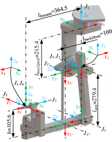
Figure 2: Frame definition of the MTM using modified DH convention.

The left and right MTMs are identical to each other, except the last four joints being mirrored to each other. Consequently, the two MTMs can be modeled similarly. The frame definition based on the modified Denavit-Hartenberg (DH) convention [18] is shown in Fig. 2, and the kinematic parameters of the MTM are described in Table I. The kinematics of the MTM can be described as

• Joint 1 rotates around the Z-axis of the base frame, $z_{0}$.

• Joints 2, 3, $3^{\prime}$, $3^{\prime\prime}$, and $3^{\prime\prime\prime}$ construct a parallelogram, which is actuated by joints 2 and $3^{\prime}$.

• Joints 4, 5, 6, and 7 form a 4-axis non-locking gimbal.

The kinematics of the MTM is fully described by the basis joint coordinates $\boldsymbol{q}^{b}$, which are equal to the dVRK joint coordinate $\boldsymbol{q}^{d}$, $\boldsymbol{q}^{b}=\boldsymbol{q}^{d}$. The additional joints $\boldsymbol{q}^{a}$ can be described as the linear combination of $\boldsymbol{q}^{b}$ by

$$\boldsymbol{q}^{a}=\begin{bmatrix}q_{3^{\prime}}&q_{3^{\prime\prime}}&q_{3^{\prime\prime\prime}}\end{bmatrix}^{\top}=\begin{bmatrix}q_{2}+q_{3}&-q_{3}&q_{3}\end{bmatrix}^{\top}$$ (1)

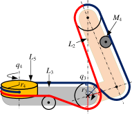
Figure 3: Modeling of the tendon coupling of the MTM.

Joints 1, 5, 6, and 7 are independently driven, and thus the motion of these joints is equivalent to their corresponding driving motors, $\boldsymbol{q}^{d}_{1,5-7}$ = $\boldsymbol{q}^{m}_{1,5-7}$. The motion of $q^{d}_{4}$ depends on both $q^{m}_{4}$ and $q^{d}_{3}$ and can be described by

$$q^{d}_{4}=q^{m}_{4}-{r_{3}}/{r_{4}}\cdot q^{d}_{3}$$ (2)

where $r_{3}\approx 14.01$ mm and $r_{4}\approx 20.92$ mm are the radii of the pulleys shown in Fig. 3.

The coupling between $\boldsymbol{q}^{d}_{2-4}$ and $\boldsymbol{q}^{m}_{2-4}$ due to the parallelogram and tendons is resolved by the coupling matrix $\boldsymbol{A}^{d}_{m}$

$$\boldsymbol{q}^{d}_{2-4}=\boldsymbol{A}^{d}_{m}\boldsymbol{q}^{m}_{2-4}=\small\begin{bmatrix}1&0&0\\ -1&1&0\\ 0.6697&-0.6697&1\end{bmatrix}\normalsize\boldsymbol{q}^{m}_{2-4}$$ (3)

II-B Kinematic Modeling of the PSM

TABLE II: Modeling Description of the PSM

$i$	$a(i)$	$a_{i-1}$	$\alpha_{i-1}$	$d_{i}$	$\theta_{i}$	$\boldsymbol{\delta}_{Li}$	$I_{mi}$	$\boldsymbol{F}_{i}$	$K_{si}$
1	0	0	$\frac{\pi}{2}$	0	$q_{1}+\frac{\pi}{2}$	✓	✕	✓	✕
2	1	0	$-\frac{\pi}{2}$	0	$q_{2}-\frac{\pi}{2}$	✓	✕	✓	✕
$2^{\prime}$	2	$l_{2L3}$	0	0	$\frac{\pi}{2}$	✕	✕	✕	✕
$2^{\prime\prime}$	$2^{\prime}$	$l_{2H1}$	0	0	$\frac{\pi}{2}-q_{2}$	✓	✕	✕	✕
$2^{\prime\prime\prime}$	$2^{\prime}$	$l_{c1}$	0	0	$\frac{\pi}{2}-q_{2}$	✓	✕	✕	✕
$2^{\prime\prime\prime\prime}$	$2^{\prime\prime}$	$l_{2L2}$	0	0	$q_{2}$	✓	✕	✕	✕
$2^{\prime\prime\prime\prime\prime}$	$2^{\prime\prime}$	$l_{2L1}$	0	0	$q_{2}+\pi$	✓	✕	✕	✕
3	$2^{\prime\prime\prime\prime}$	$l_{3}$	$-\frac{\pi}{2}$	$q_{3}+l_{c2}$	0	✓	✕	✓	✕
$3^{\prime}$	2	$l_{2L3}$	$-\frac{\pi}{2}$	$q_{3}$	0	✓	✕	✕	✕
4	3	0	0	$l_{tool}$	$q_{4}$	✕	✓	✓	✓
5	4	0	$\frac{\pi}{2}$	0	$q_{5}+\frac{\pi}{2}$	✕	✓	✓	✕
6	5	$l_{p2y}$	$-\frac{\pi}{2}$	0	$q_{6}+\frac{\pi}{2}$	✕	✕	✓	✕
7	5	$l_{p2y}$	$-\frac{\pi}{2}$	0	$q_{7}+\frac{\pi}{2}$	✕	✕	✓	✕
$M_{6}$	-	0	0	0	$q^{m}_{6}$	✕	✓	✓	✕
$M_{7}$	-	0	0	0	$q^{m}_{7}$	✕	✓	✓	✕
$F_{67}$	-	0	0	0	$q_{6}-q_{7}$	✕	✕	✓	✕

Note: Links 1 to 7 correspond to the links sescribed in Fig. 4a. $M_{6}$ and $M_{7}$ correspond to the modeling of motors 6 and 7, respectively. $F_{67}$ corresponds to the modeling of the relative motion between links 6 and 7. The dimensions are shown in Fig. 4b. $l_{c1}=l_{2H1}+l_{2H2}$, $l_{c2}=-l_{RCC}+l_{2H1}$.

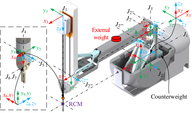
(a) Frame definition of the PSM using modified DH convention.

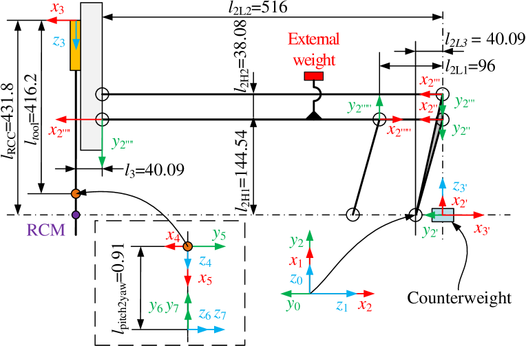
(b) Planar view of the frame definition of the PSM.

Figure 4: Frame definition of the PSM.

The frame definition of the PSM is shown in Fig. 4, and the corresponding parameters are shown in Table II. The kinematics of the PSM can be concluded as

• The first two revolute joints form a remote-center-of-motion (RCM) point via a double four-bar linkage with six links actuated by a single motor.

• The third joint is prismatic and provides the insertion of the instrument through the RCM. The first three joints allow the 3-DOF Cartesian space motion.

• Revolute joints 4 and 5 construct the roll and pitch motion of the wrist to reorient the end-effector.

• The last two joints construct the yaw motion of the end-effector, as well as the opening and closing of the gripper.

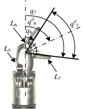
(a) Modeling of the motion of the gripper.

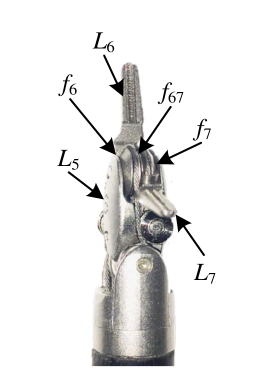
(b) Modeling of the frictions of the gripper.

Figure 5: Modeling of the gripper of the PSM.

We model the first five joints of the PSM identical to the dVRK-ROS package, i.e., $\boldsymbol{q}_{1-5}=\boldsymbol{q}^{d}_{1-5}$. The dVRK-ROS package models the last two joints as $q^{d}_{6}$, the angle from the insertion axis to the bisector of the two jaw tips, and $q^{d}_{7}$, the angle between the two jaw tips. However, the gripper jaws are designed and actuated as two separate links. As shown in Fig. 5a, the relation between $\boldsymbol{q}^{d}_{6-7}$, and $\boldsymbol{q}_{6-7}$ is described by

$$\boldsymbol{q}^{d}_{6-7}=\begin{bmatrix}q^{d}_{6}&q^{d}_{7}\end{bmatrix}^{\top}=\begin{bmatrix}0.5q_{6}+0.5q_{7}&-q_{6}+q_{7}\end{bmatrix}^{\top}$$ (4)

Since the first four joints are independently driven, the equivalent motor motion is considered to occur at joints, i.e., $\boldsymbol{q}^{d}_{1-4}=\boldsymbol{q}^{m}_{1-4}$. Based on the user guide of the dVRK, the coupling of the wrist joint actuation can be resolved by the coupling matrix $\boldsymbol{A}^{d}_{m}$ mapping $\boldsymbol{q}^{m}_{5-7}$ to $\boldsymbol{q}^{d}_{5-7}$ by

$$\boldsymbol{q}^{d}_{5-7}=\boldsymbol{A}^{d}_{m}\boldsymbol{q}^{m}_{5-7}=\small\begin{bmatrix}1.0186&0&0\\ -0.8306&0.6089&0.6089\\ 0&-1.2177&1.2177\end{bmatrix}\normalsize\boldsymbol{q}^{m}_{5-7}$$ (5)

III Dynamic Modeling of the dVRK

In this section, the dynamic parameters are described first. The dynamic equation is then formulated based on the Euler-Lagrange equation. Finally, the dynamic modeling of the MTM and PSM is introduced based on the formulation.

III-A Dynamic Parameters

Each link $k$ is characterized by the mass $m_{k}$, the center of mass (COM) relative to the link frame $k$, $\boldsymbol{r}_{k}$, and the inertia tensor about the COM, $\boldsymbol{I}_{k}$. To express the equations of motion as a linear form of dynamic parameters, we use the so-called barycentric parameters [19], in which the mass $m_{k}$ of link $k$ is first used, followed by the first moment of inertia, $\boldsymbol{l}_{k}=m_{k}\boldsymbol{r}_{k}$. Finally, the inertia tensor $\boldsymbol{L}_{k}$ about frame $k$ is used [20], which is calculated via the parallel axis theorem

$$\boldsymbol{L}_{k}=\boldsymbol{I}_{k}+m_{k}\boldsymbol{S}(\frac{\boldsymbol{l}_{k}}{m_{k}})^{\top}\boldsymbol{S}(\frac{\boldsymbol{l}_{k}}{m_{k}})=\small\begin{bmatrix}L_{kxx}&L_{kxy}&L_{kxz}\\ L_{kxy}&L_{kyy}&L_{kyz}\\ L_{kxz}&L_{kyz}&L_{kzz}\end{bmatrix}\normalsize$$ (6)

where $\boldsymbol{S}(\cdot)$ is the skew-symmetric operator.

The aforementioned inertial parameters of link $k$ are grouped into a vector $\boldsymbol{\delta}_{Lk}\in\mathbb{R}^{10}$ as

$$\boldsymbol{\delta}_{Lk}=\small[\begin{matrix}L_{kxx}&L_{kxy}&L_{kxz}&L_{kyy}&L_{kyz}&L_{kzz}&\boldsymbol{l}_{k}^{\top}&m_{k}\end{matrix}]^{\top}\normalsize$$ (7)

Besides the inertial parameters of link $k$, the corresponding joint friction coefficients, motor inertia $I_{mk}$, and spring stiffness $K_{sk}$ are grouped as additional parameters

$$\boldsymbol{\delta}_{Ak}=\begin{bmatrix}F_{vk}&F_{ck}&F_{ok}&I_{mk}&K_{sk}\end{bmatrix}^{\top}$$ (8)

where $F_{vk}$ and $F_{ck}$ are the viscous and Coulomb friction constants, and $F_{ok}$ is the Coulomb friction offset of joint $k$.

Eventually, all the parameters of $n$ joints are grouped together as the dynamic parameters $\boldsymbol{\delta}$ of a robot.

$$\boldsymbol{\delta}=\begin{bmatrix}\boldsymbol{\delta}_{L1}^{\top}&\boldsymbol{\delta}_{A1}^{\top}&...&\boldsymbol{\delta}_{Ln}^{\top}&\boldsymbol{\delta}_{An}^{\top}\end{bmatrix}^{\top}$$ (9)

III-B Dynamic Model Formulation

The inverse dynamic model for closed-chain robots, which relates motor torques and joint motion, can be calculated using Newton-Euler [21] or Euler-Lagrange [22] methods for the equivalent tree structure and by considering kinematic constraints between joint coordinates. The Euler-Lagrange equation is used to model the dynamics of the dVRK, due to its ease of dealing with kinematic constraints. The Lagrangian is calculated by the difference of the kinetic energy $K$ and potential energy $P$ of the robot, $L=K-P$. Motor inertias and springs are not included in $L$ and modeled separately.

The relation from motor motion $\boldsymbol{q}^{m}$ to the torque of each motor $i$ caused by link inertia is then computed as

$$\tau^{m}_{LIi}=\frac{\mathrm{d}}{\mathrm{d}t}\frac{\partial L}{\partial\dot{q}^{m}_{i}}-\frac{\partial L}{\partial q^{m}_{i}}$$ (10)

The friction torques of all the joints $\boldsymbol{q}^{c}$ are considered as

$$\boldsymbol{\tau}^{c}_{f}(\dot{\boldsymbol{q}}^{c})=\boldsymbol{F}_{v}\dot{\boldsymbol{q}}^{c}+\boldsymbol{F}_{c}\boldsymbol{\mathrm{sgn}}(\dot{\boldsymbol{q}}^{c})+\boldsymbol{F}_{o}$$ (11)

where $\boldsymbol{F}_{v}$ and $\boldsymbol{F}_{c}$ are diagonal matrices encapsulating the viscous and Coulomb friction constants, and $\boldsymbol{F}_{o}$ is the vector of the Coulomb friction offset constants.

The torques caused by motor inertia are defined as

$$\boldsymbol{\tau}^{m}_{MI}(\ddot{\boldsymbol{q}}^{m})=\boldsymbol{I}_{m}\ddot{\boldsymbol{q}}^{m}$$ (12)

For spring $k$, we only model the stiffness constant $K_{sk}$ as its parameter, which results into the spring torques

$$\boldsymbol{\tau}^{c}_{s}(\boldsymbol{q}^{c})=\boldsymbol{K}_{s}{\boldsymbol{\Delta l}_{s}}$$ (13)

where $\boldsymbol{K}_{s}$ is a diagonal matrix of the stiffness constants of the springs, and $\boldsymbol{\Delta l}_{s}$ is the equivalent prolongation vector.

The joint torques caused by springs and frictions can be projected onto the motor joints, using the Jacobian matrix of their corresponding joint coordinate with respect to the motor joint angle $\boldsymbol{q}^{m}$ [22]. Thus, the motor torques $\boldsymbol{\tau}^{m}$ with link inertia, springs, frictions, motor inertia, and motion couplings considered are given by

$$\boldsymbol{\tau}^{m}=\boldsymbol{\tau}^{m}_{LI}+\boldsymbol{\tau}^{m}_{MI}(\ddot{\boldsymbol{q}}^{m})+\frac{\partial{\boldsymbol{q}^{c}}}{\partial\boldsymbol{q}_{m}}(\boldsymbol{\tau}^{c}_{s}(\boldsymbol{q}^{c})+\boldsymbol{\tau}^{c}_{f}(\dot{\boldsymbol{q}}^{c}))$$ (14)

To identify $\boldsymbol{\delta}$, (14) is rewritten into (15) by the linear parameterization.

$$\boldsymbol{\tau}^{m}=\boldsymbol{H}(\boldsymbol{q}^{m},\dot{\boldsymbol{q}}^{m},\ddot{\boldsymbol{q}}^{m})\boldsymbol{\delta}$$ (15)

QR decomposition with pivoting [23] is used to calculate the base parameters, a minimum set of dynamic parameters that can fully describe the dynamic model of a robot. With this method, we get a permutation matrix $\boldsymbol{P}_{\mathrm{b}}\in\boldsymbol{\mathbb{R}}^{n\times b}$, where $n$ is the number of standard dynamic parameters and $b$ is the number of base parameters. The base parameters $\boldsymbol{\delta}_{\mathrm{b}}$ and the corresponding regressor $\boldsymbol{H}_{\mathrm{b}}$ can then be calculated by

$$\boldsymbol{\delta}_{\mathrm{b}}=\boldsymbol{P}_{\mathrm{b}}^{\top}\boldsymbol{\delta},\,\,\,\,\boldsymbol{H}_{\mathrm{b}}=\boldsymbol{H}\boldsymbol{P}_{\mathrm{b}}$$ (16)

III-C Dynamic Modeling of the MTM

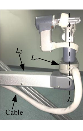
(a) Electrical cable on joint 4 of the MTM.

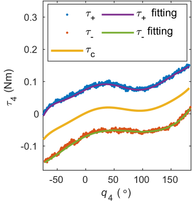
(b) Modeling of the joint torque from the electrical cable on joint 4.

Figure 6: Modeling of the joint torque from the electrical cable on joint 4 of the MTM.

The dynamic modeling description for the MTM is shown in Table I. All the nine links are modeled with link inertia. The frictions of all the joints $\boldsymbol{q}$ are considered, except joint $3^{\prime\prime\prime}$ since joint $3^{\prime\prime\prime}$ and joint $3^{\prime\prime}$ share the same joint coordinate, and their frictions are coupled together. Similarly, all the motors except the $\nth{4}$ one have their corresponding independently driven joints which have already been modeled with link inertia and joint friction. Therefore, only motor 4 is modeled with motor inertia and motor friction.

The electrical cable along joint 4 (Fig. 6a) affects its joint torque significantly. The joint torque data of joint 4, $\tau_{4}^{+}$ and $\tau^{-}_{4}$, was collected, with joint 4 rotating at $\pm 0.4$ rad/s and other joints being stationary, as shown in Fig. 6b. We collected data at constant joint velocities, which explicitly removes any torque due to inertia. Moreover, due to the friction model in (11), the frictions with the joint velocity at $\pm 0.4$ rad/s should be opposite to each other if the Coulomb friction offset is not considered. Thus finally, we computed the mean of $\tau_{4}^{+}$ and $\tau^{-}_{4}$, which canceled the viscous and Coulomb friction terms and kept the joint friction offset and torque applied to the joint from the cable physically acting on it, $\tau^{m}_{c4}(q_{4})$.

To get $\tau^{m}_{c4}(q_{4})$, we first fitted the joint torque data at $\pm 0.4$ rad/s using $\nth{7}$ order polynomial functions of $q_{4}$, respectively, as shown in Fig. 6b. Next, the mean of the obtained coefficients of the two polynomials $\boldsymbol{p}_{4}^{+}$ and $\boldsymbol{p}_{4}^{-}$ was calculated as the coefficients of the polynomial that represents $\tau^{m}_{c4}(q_{4})$.

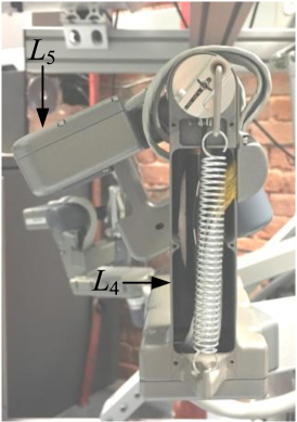
(a) Spring on joint 5.

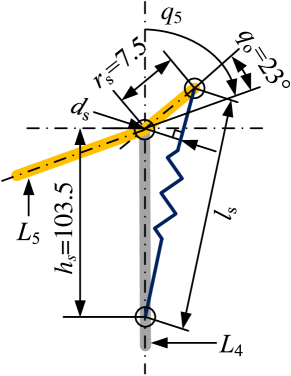
(b) Modeling of the spring.

Figure 7: Spring on joint 5 of the MTM and its modeling.

In addition, on joint 5 of the MTM, there is a spring to balance the gravitational force (Fig. 7a). Due to the modeling shown in Fig. 7b, the joint torque from the spring is given by

$$\tau_{s5}=f_{s}\cdot d_{s}=K_{s5}(l_{s}-l_{r})\cdot d_{s}=K_{s5}\Delta l_{s5}$$ (17)

where $l_{s}$ is the length between the two axes connecting the spring, which can be calculated using the law of sines as

$$l_{s}=\sqrt[]{h_{s}^{2}+r_{s}^{2}-2h_{s}r_{s}\cos(\pi+q_{o}-q_{5})}$$ (18)

and $l_{r}\approx 61.3$ mm by measurement is the value of $l_{s}$ when the spring is relaxed. Based on basic trigonometry, the moment arm $d_{s}$ can be calculated by

$$d_{s}=h_{s}r_{s}\sin(\pi+q_{o}-q_{5})/l_{s}$$ (19)

where $h_{s}$, $r_{s}$ and $q_{o}$ are constants shown in Fig. 7b.

Thus, $\Delta l_{s5}=(l_{s}-l_{r})d_{s}$.

III-D Dynamic Modeling of the PSM

The dynamic modeling description of the PSM is shown in Table II. Inertia is considered for all the links contributing to the Cartesian motion, including the counterweight, link $3^{\prime}$. The motor inertia of these joints is ignored since it is not significant compared to their link inertia. The inertia of the wrist and gripper links is minimal, and thus infeasible to identify. Therefore, we only model the inertia of motors for the wrist and gripper, corresponding to the motion of $\boldsymbol{q}^{m}_{4-7}$.

Since joints $2$, $2^{\prime\prime}$, $2^{\prime\prime\prime}$, $2^{\prime\prime\prime\prime}$, and $2^{\prime\prime\prime\prime\prime}$ are all driven by a single motor, their frictions can be represented by the friction of one joint for simplicity. Thus, among these joints, only joint 2 is modeled with friction. Similarly, only joint 3 is modeled with friction out of joints 3 and $3^{\prime}$. Because of the contact between links 5 and 6, and between links 5 and 7, as shown in Fig. 5b, the frictions on joints 6 and 7 are modeled, corresponding to the motion of $q_{6}$ and $q_{7}$. Moreover, the friction between links 6 and 7 due to the contact between the two jaw tips is considered, corresponding to the motion of $q_{7}-q_{6}$. Additionally, the frictions on the motor sides of the last four joints are also modeled, corresponding to the motor motion of $\boldsymbol{q}^{m}_{4-7}$.

The torsional spring on joint 4 which rotates the joint back to its home position is modeled as

$$\tau_{s4}=K_{s4}(-q_{4})=K_{s4}\Delta l_{s4}$$ (20)

IV Excitation Trajectory Optimization

Periodic excitation trajectories based on Fourier series [24] are used to generate data for dynamic model identification. These trajectories minimize the condition number of the regression matrix $\boldsymbol{W}_{b}$ for the base parameters $\boldsymbol{\delta}_{\mathrm{b}}$, which decide the dynamic behavior of a robot.

$$\boldsymbol{W}_{b}=\small\begin{bmatrix}\boldsymbol{H}_{b}(\boldsymbol{q}^{m}_{1},\dot{\boldsymbol{q}}^{m}_{1},\ddot{\boldsymbol{q}}^{m}_{1})\\ \boldsymbol{H}_{b}(\boldsymbol{q}^{m}_{2},\dot{\boldsymbol{q}}^{m}_{2},\ddot{\boldsymbol{q}}^{m}_{2})\\ \vdots\\ \boldsymbol{H}_{b}(\boldsymbol{q}^{m}_{S},\dot{\boldsymbol{q}}^{m}_{S},\ddot{\boldsymbol{q}}^{m}_{S})\\ \end{bmatrix}\normalsize$$ (21)

where $\boldsymbol{q}^{m}_{i}$ is the motor joint coordinate at $i^{\mathrm{th}}$ sampling point and $S$ is the number of sampling points.

The joint coordinate $q^{m}_{k}$ of motor $k$ can be calculated by

$$q^{m}_{k}(t)=q^{m}_{ok}+\sum_{l=1}^{n_{\mathrm{H}}}\frac{a_{lk}}{\omega_{f}l}\sin(\omega_{f}lt)-\frac{b_{lk}}{\omega_{f}l}\cos(\omega_{f}lt)$$ (22)

where $\omega_{f}=2\pi f_{f}$ is the angular component of the fundamental frequency $f_{f}$, $n_{\mathrm{H}}$ is the harmonic number of Fourier series, $a_{lk}$ and $b_{lk}$ are the amplitudes of the $l^{\mathrm{th}}$-order sine and cosine functions, $q^{m}_{ok}$ is the position offset, and $t$ is the time.

The motor joint velocity $\dot{q}^{m}_{k}(t)$ and acceleration $\ddot{q}^{m}_{k}(t)$ can be calculated easily by the differentiation of $q^{m}_{k}(t)$. And the trajectory must satisfy the following constraints:

• The joint position $\boldsymbol{q}$ is between the lower bound $\boldsymbol{q}_{l}$ and the upper bound $\boldsymbol{q}_{u}$, $\boldsymbol{q}_{l}\leq\boldsymbol{q}\leq\boldsymbol{q}_{u}$.

• The absolute value of the joint velocity $\dot{\boldsymbol{q}}$ is smaller than its maximum value $\dot{\boldsymbol{q}}_{max}$, $|\dot{\boldsymbol{q}}|<\dot{\boldsymbol{q}}_{max}$.

• The robot is confined in its workspace. The Cartesian position $\boldsymbol{p}_{k}$ of frame $k$ is between its lower bound $\boldsymbol{p}_{lk}$ and upper bound $\boldsymbol{p}_{uk}$, $\boldsymbol{p}_{lk}\leq\boldsymbol{p}_{k}\leq\boldsymbol{p}_{uk}$.

V Identification

To identify the dynamic parameters, we move the robot along the excitation trajectories generated via the method described in Section IV. Data is collected at each sampling time to obtain the regression matrix $\boldsymbol{W}$ and the dependent variable vector $\boldsymbol{\omega}$.

$$\boldsymbol{W}=\small\begin{bmatrix}\boldsymbol{H}(\boldsymbol{q}^{m}_{1},\dot{\boldsymbol{q}}^{m}_{1},\ddot{\boldsymbol{q}}^{m}_{1})\\ \boldsymbol{H}(\boldsymbol{q}^{m}_{2},\dot{\boldsymbol{q}}^{m}_{2},\ddot{\boldsymbol{q}}^{m}_{2})\\ \vdots\\ \boldsymbol{H}(\boldsymbol{q}^{m}_{\mathrm{S}},\dot{\boldsymbol{q}}^{m}_{S},\ddot{\boldsymbol{q}}^{m}_{S})\\ \end{bmatrix}\normalsize,\>\boldsymbol{\omega}=\small\begin{bmatrix}\boldsymbol{\tau}^{m}_{1}\\ \boldsymbol{\tau}^{m}_{2}\\ \vdots\\ \boldsymbol{\tau}^{m}_{S}\\ \end{bmatrix}\normalsize$$ (23)

where $\boldsymbol{\tau}^{m}_{i}$ is the motor torque at $i^{\mathrm{th}}$ sampling point.

The identification problem can then be formulated into an optimization problem which minimizes the squared residual error $||\boldsymbol{\epsilon}||^{2}$ w.r.t. the decision vector $\boldsymbol{\delta}$.

$$||\boldsymbol{\epsilon}||^{2}=||\boldsymbol{W}\boldsymbol{\delta}-\boldsymbol{\omega}||^{2}$$ (24)

To get more realistic dynamic parameters and reduce overfitting problems [17], we utilize physical consistency constraints for dynamic parameters:

• The mass of each link $k$ is positive, $m_{k}>0$.

• The inertia matrix of each link $k$ is positive definite, $\boldsymbol{I}_{k}\succ\boldsymbol{0}$ [15], and its eigenvalues, $Y_{x}$, $Y_{y}$, and $Y_{z}$, should follow the so-called triangle inequality conditions [16], i.e., $Y_{x}+Y_{y}>Y_{z}$, $Y_{y}+Y_{z}>Y_{x}$, and $Y_{z}+Y_{x}>Y_{y}$.

• The COM of link $k$, $\boldsymbol{r}_{k}$, is inside its convex hull, $m_{k}\boldsymbol{r}_{lk}-\boldsymbol{l}_{k}\leq 0$ and $m_{k}\boldsymbol{r}_{uk}+\boldsymbol{l}_{k}\leq 0$, where $\boldsymbol{r}_{lk}$ and $\boldsymbol{r}_{uk}$ are the lower and upper bounds of $\boldsymbol{r}_{k}$, respectively [10].

• The viscous and Coulomb friction coefficients for each joint $i$ are positive, $F_{vi}>0$ and $F_{ci}>0$.

• The inertia of motor $k$ is positive, $I_{mk}>0$.

• The stiffness of spring $k$ is positive, $K_{k}>0$.

The first two constraints regarding the inertia properties of link $k$ can be derived into an equivalent with LMIs [14] as

$$\boldsymbol{\bar{D}}_{k}(\boldsymbol{\delta}_{Lk})=\small\begin{bmatrix}\frac{1}{2}\mathrm{tr}(\boldsymbol{L}_{k})\cdot\boldsymbol{1}_{3}-\boldsymbol{L}_{k}&\boldsymbol{l}_{k}\\ \boldsymbol{l}_{k}^{\top}&m_{k}\end{bmatrix}\normalsize\succ\boldsymbol{0}$$ (25)

We can also add the lower and upper bounds to $m_{k}$, $F_{vi}$, $F_{ci}$ and $K_{j}$ when we have more knowledge about them.

VI Experiments

This section presents the experimental procedures and results of the dynamic model identification of the dVRK arms.

VI-A Experimental Procedures

VI-A1 Excitation Trajectory Generation

Two independent excitation trajectories were generated for identification and test, respectively, for each of the MTM and PSM. The harmonic number $n_{H}$ was set to 6. The fundamental frequency $f_{f}$ of the MTM and PSM were 0.1 and 0.18 Hz, respectively. The joint position and velocity were constrained within their ranges in the optimization. Since links $2^{\prime\prime}$ and $2^{\prime\prime\prime}$ of the PSM are very close to each other with similar motion, it is hard to get a trajectory with a low condition number of $\boldsymbol{W}_{b}$ when both links $2^{\prime\prime}$ and $2^{\prime\prime\prime}$ are considered. Links 2 and $2^{\prime\prime\prime\prime\prime}$ have the similar problem. Therefore, the trajectory optimization of the PSM was based on the model without links $2^{\prime\prime\prime}$ and $2^{\prime\prime\prime\prime\prime}$. Finally, pyOpt [25] was used to solve this constrained nonlinear optimization problem.

VI-A2 Data Collection and Processing

The joint position, velocity, and torque were collected at 200 Hz in position control mode. The joint acceleration was obtained by the second-order numerical differentiation of the velocity. A sixth-order low-pass filter was used to filter the data with the cutoff frequencies of 1.8 Hz for the MTM and 5.4 Hz for the PSM. The cutoff frequencies were chosen experimentally to achieve the best identification performance as they are low enough to filter the noise as well as high enough to keep the useful signal in the collected data. To achieve zero phase delay, we applied this filter in both forward and backward directions.

VI-A3 Identification

To get uniformly precise identification results for all joints, the residual error $\boldsymbol{\epsilon}_{i}$ of each motor joint $i$ in (24) was weighted by $w_{i}=1/(\max\{\boldsymbol{\tau}^{m}_{i}\}-\min\{\boldsymbol{\tau}^{m}_{i}\})$. As a convex optimization problem, the identification was solved via the CVXPY package [26] with the SCS solver [27].

VI-B Validation of the Identified Values

VI-B1 Identification for the dVRK Arms

The identified dynamic parameters $\hat{\boldsymbol{\delta}}$ from identification trajectories were used to predict the motor joint torque on test trajectories, $\hat{\boldsymbol{\omega}}=\boldsymbol{W}\hat{\boldsymbol{\delta}}$. The relative root mean squared error was used as the relative prediction error to assess the identification quality, $\boldsymbol{\epsilon}=||\boldsymbol{\omega}-\hat{\boldsymbol{\omega}}||_{2}/{||\boldsymbol{\omega}||_{2}}$. The same experimental procedure was conducted with the modeling from [6] for comparision since it is the only previous work considering physical consistency.

TABLE III: Relative Prediction Error on Test Trajectories

	$\tau^{m}_{1}$	$\tau^{m}_{2}$	$\tau^{m}_{3}$ or $f^{m}_{3}$	$\tau^{m}_{4}$	$\tau^{m}_{5}$	$\tau^{m}_{6}$	$\tau^{m}_{7}$
MTM-Y (%)	7.6	14.9	17.0	22.3	28.0	23.4	34.0
MTM-F (%)	11.5	18.6	40.0	36.2	69.3	31.1	37.0
PSM-Y (%)	9.3	17.8	19.1	13.4	23.9	21.3	26.4
PSM-F (%)	10.6	18.8	18.9	88.7	87.8	72.2	36.5

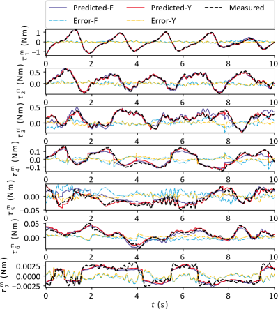
Figure 8: Measured and predicted torques on the test trajectory of the MTM.

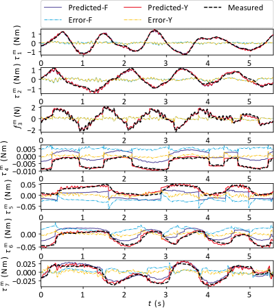
Figure 9: Measured and predicted torques on the test trajectory of the PSM.

Fig. 8 and 9 show the comparison of the measured and predicted torques on the test trajectories for the MTM and PSM, respectively. The relative prediction error of each motor joint is shown in Table III. The suffixes, -F and -Y, represent the modeling from [6] and our work, respectively.

For our proposed approach, the relative prediction errors of the first three motor joints of the MTM are less than $17.0\%$, which correspond to the Cartesian motion and most of the link inertia of the MTM. The large backlash from gearboxes and small link inertia of the last four joints make it hard to identify their dynamic parameters accurately. Hence, the relative prediction errors of the last four motor joints are relatively higher. Compared to the method from [6], our proposed approach achieves better overall identification performance. Particularly, incorporating the modeling of the nonlinear friction on joint 4 and the spring on joint 5 improves the identification performance for joints 4 and 5, significantly.

For our proposed approach, the relative prediction error of the first three motor joints of the PSM is less than $19.1\%$, which correspond to the Cartesian motion and most of the link inertia of the arm. The relative prediction errors of the last four motor joints are relatively larger since they are only modeled with motor inertia and frictions, and the magnitudes of the joint torques are very small. Compared to the method from [6], our proposed approach achieves similar identification performance for the first three joints while much better performance for the last four joints. This improvement is owed to the modeling of friction offset (see joints 4 and 5 in Fig. 9) and motor inertia.

VI-B2 Identification with a Weight on the PSM

The same identification procedure was performed with a standard 200 g weight (totally 205 g, with 5 g tapes added) firmly taped on the top of the parallelogram of the PSM, i.e., link $2^{\prime\prime}$ (see Fig. 4). We listed all the seven base parameters related to $m_{2^{\prime\prime}}$ in Table IV. Since each complete symbolic base parameter is too long to show here, we only show part of it to illustrate the relation between the parameter and $m_{2^{\prime\prime}}$.

With the values of one parameter identified with and without the weight (i.e., $\hat{\delta}_{b}$ and $\hat{\delta}_{b}^{w}$), we estimated the mass of the weight as, $\hat{m}_{w}=(\hat{\delta}_{b}^{w}-\hat{\delta}_{b})/c_{m_{2^{\prime\prime}}}$, where $c_{m_{2^{\prime\prime}}}$ is the coefficient of the corresponding $m_{2^{\prime\prime}}$ term. The relative estimation error of the weight was calculated by $\epsilon_{w}=|\hat{m}_{w}-205|/205$. As shown in Table IV, the low $\epsilon_{w}$ was achieved through most parameters, except the $5^{\mathrm{th}}$ one whose $\epsilon_{w}$ is as high as 82.5%. This can be caused by identification noise. The $c_{m_{2^{\prime\prime}}}$ of this parameter is only 0.00576, which is much smaller than the $c_{m_{2^{\prime\prime}}}$ of other parameters, and thus $\hat{m}_{w}$ is more sensitive to noise for this parameter. In summary, the overall accurate estimation of the mass of the weight further demonstrates the robustness of the proposed approach and package.

TABLE IV: Comparison of the $m_{2^{\prime\prime}}$-Related Base Parameters Identified with and without the Weight

base parameter related to $m_{2^{\prime\prime}}$	$\hat{\delta}_{b}$	$\hat{\delta}_{b}^{w}$	$\hat{m}_{w}$ (g)	$\epsilon_{w}$ (%)
$-0.5l_{2y}-0.072m_{2^{\prime\prime}}+\ldots$	0.06147	0.04668	204.6	0.2
$0.5l_{2x}+0.020m_{2^{\prime\prime}}+\ldots$	-0.01895	-0.01437	228.2	1.1
$0.5l_{2y}+0.072m_{2^{\prime\prime}}+\ldots$	-0.1324	-0.1177	203.2	0.9
$-0.5l_{2x}-0.020m_{2^{\prime\prime}}+\ldots$	0.02080	0.01725	176.9	13.7
$L_{2xy}+0.00576m_{2^{\prime\prime}}+\ldots$	-0.05245	-0.05038	35.9	82.5
$L_{2xx}-0.0415m_{2^{\prime\prime}}+\ldots$	0.2068	0.1995	176.2	14.0
$L_{2zz}-0.0415m_{2^{\prime\prime}}+\ldots$	0.2390	0.2307	198.0	3.4

VII Conclusion

In this work, an open-source software package for the dynamic model identification of the dVRK is presented. Link inertia, joint friction, springs, tendon couplings, cable force, and closed-chains are incorporated in the modeling. Fourier series-based trajectories are used to excite the dynamics of the dVRK, with the condition number of the regression matrix minimized. A convex optimization-based method is used to obtain dynamic parameters subject to physical consistency constraints. Experimental results show the improvement of the proposed modeling and the robustness of the package. Although this software package is developed for the dVRK, it is feasible to use it on other robots.

Despite the improvement of identification performance in our modeling compared to [6], we can still observe substantial deviations between the measured and predicted torques. Although the convex optimization-based framework ensures the global optimality of identification results, it relies on the linearity of dynamic parameters w.r.t. joint torques [10]. As a result, nonlinear friction models considering presliding hysteresis, such as the Dahl model [28], which can potentially improve the modeling of electrical cables and tendon-sheath transmission, cannot be used in this package. Moreover, the present identification approach requires the computation of acceleration, which provides more information, however, requires correct handling of data filtering, compared to energy model-based methods [29].

References

- [1] Peter Kazanzides et al. “An open-source research kit for the da Vinci® Surgical System” In IEEE Int. Conf. on Robotics and Automation, 2014, pp. 6434–6439
- [2] G. A. Fontanelli et al. “A V-REP simulator for the da Vinci research kit robotic platform” In IEEE Int. Conf. on Biomedical Robotics and Biomechatronics, 2018, pp. 1056–1061
- [3] Florian Richter, Ryan K Orosco and Michael C Yip “Open-Sourced Reinforcement Learning Environments for Surgical Robotics” In arXiv preprint arXiv:1903.02090, 2019
- [4] Fernando Reyes and Rafael Kelly “Experimental evaluation of model-based controllers on a direct-drive robot arm” In Mechatronics 11.3 Elsevier, 2001, pp. 267–282
- [5] Alessandro De Luca, Alin Albu-Schaffer, Sami Haddadin and Gerd Hirzinger “Collision detection and safe reaction with the DLR-III lightweight manipulator arm” In IEEE/RSJ Int. Conf. on Intelligent Robots and Systems, 2006, pp. 1623–1630
- [6] Giuseppe Andrea Fontanelli, Fanny Ficuciello, Luigi Villani and Bruno Siciliano “Modelling and identification of the da Vinci research kit robotic arms” In IEEE/RSJ Int. Conf. on Intelligent Robots and Systems, 2017, pp. 1464–1469
- [7] Hongqiang Sang et al. “External force estimation and implementation in robotically assisted minimally invasive surgery” In The Int. J. of Medical Robotics and Computer Assisted Surgery 13.2 Wiley Online Library, 2017, pp. e1824
- [8] Radian A Gondokaryono “Cooperative Object Manipulation with Force Tracking on the da Vinci Research Kit”, 2018
- [9] Francesco Piqué et al. “Dynamic Modeling of the da Vinci Research Kit Arm for the Estimation of Interaction Wrench” In IEEE Int. Symposium on Medical Robotics, 2019, pp. 1–7
- [10] Cristóvão D Sousa and Rui Cortesão “Physical feasibility of robot base inertial parameter identification: A linear matrix inequality approach” In The Int. J. of Robotics Research 33.6, 2014, pp. 931–944
- [11] Cristóvão Duarte Sousa “SymPyBotics V1.0” Zenodo, 2014 DOI: 10.5281/zenodo.11365
- [12] Stefan Bethge, Jörn Malzahn, Nikolaos Tsagarakis and Darwin Caldwell “FloBaRoID - A software package for the identification of robot dynamics parameters” In Int. Conf. on Robotics in Alpe-Adria Danube Region, 2017, pp. 156–165
- [13] Wisama Khalil et al. “OpenSYMORO: An open-source software package for Symbolic Modelling of Robots” In IEEE/ASME Int. Conf. on Advanced Intelligent Mechatronics, 2014, pp. 1206–1211
- [14] Patrick M Wensing, Sangbae Kim and Jean-Jacques E Slotine “Linear matrix inequalities for physically consistent inertial parameter identification: A statistical perspective on the mass distribution” In IEEE Robotics and Automation Letters 3.1, 2018, pp. 60–67
- [15] Koji Yoshida and Wisama Khalil “Verification of the positive definiteness of the inertial matrix of manipulators using base inertial parameters” In The Int. J. of Robotics Research 19.5, 2000, pp. 498–510
- [16] Silvio Traversaro, Stanislas Brossette, Adrien Escande and Francesco Nori “Identification of fully physical consistent inertial parameters using optimization on manifolds” In IEEE/RSJ Int. Conf. on Intelligent Robots and Systems, 2016, pp. 5446–5451
- [17] Cristóvão D Sousa and Rui Cortesao “Inertia Tensor Properties in Robot Dynamics Identification: A Linear Matrix Inequality Approach” In IEEE/ASME Trans. on Mechatronics 24.1, 2019, pp. 406–411
- [18] Wisama Khalil and J. Kleinfinger “A new geometric notation for open and closed-loop robots” In IEEE Int. Conf. on Robotics and Automation 3, 1986, pp. 1174–1179
- [19] Pascal Maes, J-C Samin and P-Y Willems “Linearity of multibody systems with respect to barycentric parameters: Dynamics and identification models obtained by symbolic generation” In Mechanics of Structures and Machines 17.2 Taylor & Francis, 1989, pp. 219–237
- [20] Wisama Khalil and Etienne Dombre “Modeling, identification and control of robots” Butterworth-Heinemann, 2004
- [21] Wisama Khalil “Dynamic modeling of robots using recursive Newton-Euler techniques” In ICINCO2010, 2010
- [22] Yoshihiko Nakamura and Modjtaba Ghodoussi “Dynamics computation of closed-link robot mechanisms with nonredundant and redundant actuators” In IEEE Trans. on Robotics and Automation 5.3, 1989, pp. 294–302
- [23] Maxime Gautier “Numerical calculation of the base inertial parameters of robots” In J. of Field Robotics 8.4 Wiley Online Library, 1991, pp. 485–506
- [24] Jan Swevers et al. “Optimal robot excitation and identification” In IEEE Trans. on Robotics and Automation 13.5, 1997, pp. 730–740
- [25] Ruben E. Perez, Peter W. Jansen and Joaquim R. R. A. Martins “pyOpt: A Python-Based Object-Oriented Framework for Nonlinear Constrained Optimization” In Structures and Multidisciplinary Optimization 45.1, 2012, pp. 101–118 DOI: 10.1007/s00158-011-0666-3
- [26] Steven Diamond and Stephen Boyd “CVXPY: A Python-Embedded Modeling Language for Convex Optimization” In J. of Machine Learning Research 17.83, 2016, pp. 1–5
- [27] B. O’Donoghue, E. Chu, N. Parikh and S. Boyd “SCS: Splitting Conic Solver, version 2.0.2”, https://github.com/cvxgrp/scs, 2017
- [28] Phil R Dahl “A solid friction model”, 1968
- [29] Maxime Gautier and Wisama Khalil “On the identification of the inertial parameters of robots” In IEEE Conf. on Decision and Control, 1988, pp. 2264–2269