Nonlinear Instability of Periodic Traveling Waves

Abstract

We study the local dynamics of $L^{2}\left(\mathbb{R}\right)$-perturbations to the zero solution of spatially $2\pi$-periodic coefficient reaction-diffusion systems. In this case the spectrum of the linearization about the zero solution is purely essential and may be described via the point spectrum of a one-parameter family of Bloch operators. When this essential spectrum is unstable, we characterize a large class of initial perturbations which lead to nonlinear instability of the trivial solution. This is accomplished by using the Bloch transform to construct an appropriate projection to capture the maximum amount of linear exponential growth associated to the initial perturbation arising from the unstable eigenvalues of the Bloch operators. This result is also extended to dissipative systems of conservation laws.

1 Introduction

We consider a reaction-diffusion type system of real-valued differential equations of the form

$$\left\{\begin{aligned} u_{t}\left(x,t\right)&=Lu\left(x,t\right)+\mathcal{N}\left(u\left(x,t\right)\right)\\ u\left(x,0\right)&=u_{0}\left(x\right)\end{aligned}\right.\qquad\begin{array}[]{c}x\in\mathbb{R},\ t>0\\ u\in\mathbb{R}^{d}\end{array}$$ (1.1)

posed on $X=H^{n}\left(\mathbb{R}\right)$, an appropriate Sobolev subspace of $L^{2}\left(\mathbb{R}\right)$, where $L$ is an $2n$-th order linear differential operator of the form

$$L=\sum_{j=0}^{2n}a_{j}\left(x\right)\partial_{x}^{j}$$ (1.2)

with real-valued $2\pi$-periodic coefficient functions $a_{j}\left(x\right)$. Other periods may be considered by rescaling $x$. For simplicity we also assume that $L$ is a sectorial operator. We assume the nonlinear operator $\mathcal{N}$ satisfies the following polynomial estimate,

$$\left\|\mathcal{N}\left(u\right)\right\|_{X}\leq\left\|u\right\|_{X}^{p}\qquad\text{for some }p>1.$$ (1.3)

Systems of the form (1.1) naturally arise when considering the local dynamics of constant coefficient systems of reaction-diffusion systems near a spatially-periodic equilibrium solution. That is, supposing an evolution equation $y_{t}=\mathcal{F}\left(y\right)$ has a spatially-periodic equilibrium solution $\phi$, with $\mathcal{F}\left(\phi\right)=0$, we investigate the behavior of solutions that begin as small perturbations of $\phi$, i.e. solutions with initial conditions of the form $y_{0}=\phi+u_{0}$. Typically one writes the solution as $y\left(x,t\right)=\phi\left(x\right)+u\left(x,t\right)$, substitutes this ansatz into $\mathcal{F}\left(y\right)$, then uses the condition $\mathcal{F}\left(\phi\right)=0$ to find the “perturbation equations” that govern the evolution of the perturbation $u$. In this case equation (1.1) would specifically be this perturbation equation.

For the local dynamics, we use the following definition of stability,

Definition 1.

Let $\phi$ be an equilibrium solution and $u$ be a perturbation (as above) which satisfies (1.1). The equilibrium solution $\phi$ is said to be stable (in the norm $\left\|\cdot\right\|$) if for all $\epsilon>0$ there exists a $\eta>0$ so that requiring $\left\|u_{0}\right\|<\eta$ ensures that $\left\|u\left(t\right)\right\|<\epsilon$ for all time. Otherwise $\phi$ is said to be unstable.

Traditionally the focus has been showing that equilibrium solutions are stable. In contrast, we are particularly interested in the case when the $L^{2}\left(\mathbb{R}\right)$ spectrum of $L$, $\sigma\left(L\right)$, is “spectrally unstable”: when $\sigma\left(L\right)\cap\left\{z\in\mathbb{C}\ \middle|\ \text{Re }z>0\right\}\neq\emptyset$. In [8, 9] it is shown that spectral instability leads to instability. This is done by constructing a specific initial perturbation $u_{0}$ which results in a poorly behaved solution, thus precluding stability. In particular in [9] the initial perturbation $u_{0}$ is taken to be a perturbation which “activates” the most unstable part of $\sigma\left(L\right)$, roughly speaking that it projects into the most unstable subspaces.

Where this paper differs is that we allow the initial perturbations $u_{0}$ to be as arbitrary as possible and attempt to characterize which could be used to preclude stability. To this end, we define stability for an initial perturbation $u_{0}$ (in contrast to an equilibrium solution $\phi$).

Definition 2.

An initial perturbation $u_{0}$ of (1.1) is said to be stable (in the norm $\left\|\cdot\right\|$) if for all $\epsilon>0$ there exists an $\eta>0$ so that for all $0<\delta<\eta$, if $u_{\delta}$ is the solution to (1.1) with initial perturbation $\delta u_{0}$, then $\left\|u_{\delta}\left(t\right)\right\|<\epsilon$ for all time. Otherwise $u_{0}$ is said to be unstable.

With this definition in mind, [9] shows that the initial perturbation which activates the rightmost part of $\sigma\left(L\right)$ is unstable. But what if an initial perturbation activates any other part of $\sigma\left(L\right)\cap\left\{z\in\mathbb{C}\ \middle|\ \text{Re }z>0\right\}$? A naive guess would be that if $u_{0}$ activates $\sigma\left(L\right)\cap\left\{z\in\mathbb{C}\ \middle|\ \text{Re }z>0\right\}$ it is unstable, and if it does not it is stable. If that were the case, then one would obtain stability of $\phi$ for a wide range of initial perturbations.

Our main result is a step in this direction with Theorem 7 which concludes that if an initial perturbation activates an appropriate subset of $\sigma\left(L\right)\cap\left\{z\in\mathbb{C}\ \middle|\ \text{Re }z>0\right\}$, then that initial perturbation is unstable. This result applies to many reaction-diffusion type systems with periodic equilibrium solutions, including but not limited to scalar reaction diffusion, FitzHugh-Nagumo [14], the Klausmeier model for vegetation stripe formulation [18, 17], and the Belousov-Zhabotinskii reaction [4]. This methodology is robust enough that in Theorem 10 we show how it may be extended to dissipative systems of conservation laws such as Kuramoto-Sivashinsky [3, 10] and the St. Venant equation [2, 15].

To see how a spectral instability may lead to a nonlinear instability, we recall from Duhamel’s equation the solution of (1.1) can be decomposed as

$$u\left(x,t\right)=e^{Lt}u_{0}\left(x\right)+\int_{0}^{t}e^{L\left(t-s\right)}\mathcal{N}\left(u\left(x,s\right)\right)\ ds\,,$$ (1.4)

which uses the solution semigroup $e^{Lt}$ to write the solution in terms of a linear part and a nonlinear part.

The stability of the linear part is directly influenced by point spectrum of $L$. Suppose $L$ had an eigenfunction $\psi$ with eigenvalue $\lambda$ with $\text{Re }\lambda>0$: then choosing $\psi$ as an initial perturbation, the linear part would be $e^{\lambda t}\psi$ and we would have exponential growth. While in general the $L^{2}\left(\mathbb{R}\right)$ spectrum of $L$ will not contain such eigenvalues, as the coefficient functions $a_{j}\left(x\right)$ in (1.2) were taken to be $2\pi$-periodic then Floquet theory gives the $L^{2}\left(\mathbb{R}\right)$ spectrum of $L$ as the collection of $L_{\text{per}}^{2}[0,2\pi)$ point spectrum of the one-parameter family of operators $L_{\xi}=e^{-i\xi x}Le^{i\xi x}$ with $\xi\in\left[-\frac{1}{2},\frac{1}{2}\right)$ [11, Proposition 3.1]. The respective domains $L^{2}\left(\mathbb{R}\right)$ and $L_{\text{per}}^{2}[0,2\pi)$ are connected through the Bloch Transform. (This theory and its preliminaries are developed in Subsection 2.1, and that specific spectral result is given in Proposition 3). In Subsection 2.2 we use the Bloch Transform to define the projection (2.10) which allow us to use this unstable point spectrum of $L_{\xi}$ to conclude exponential growth for the linear part of (1.4).

This clarifies the notion of “$u_{0}$ activating an unstable part of $\sigma\left(L\right)$” as “the Bloch Transform of $u_{0}$ contains some sufficiently unstable eigenspace of some $L_{\xi}$.” A further area of study would be to see if this Bloch transform view gives any insight into specifically how the initial perturbation goes unstable.

To handle the nonlinear part of (1.4), we apply the reverse triangle inequality to obtain the following lower bound for the solution,

$$\left|\left\|e^{Lt}u_{0}\right\|_{X}-\left\|\int_{0}^{t}e^{L\left(t-s\right)}\mathcal{N}\left(u\left(x,s\right)\right)\ ds\right\|_{X}\right|\leq\left\|u\left(x,t\right)\right\|_{X}\,.$$ (1.5)

In Section 3 we prove an upper bound on the growth of the nonlinear part, which when contrasted with the exponential growth of the linear part gives instability.

2 Spectral Properties

2.1 Characterization of the Spectrum

The operator $L$ from (1.1) is a linear differential operator with $2\pi$-periodic coefficients, so standard results in Floquet theory [5, Section 2.4] tell us that there are no $L^{2}\left(\mathbb{R}\right)$ eigenfunctions: the spectrum is entirely essential. Furthermore, the spectrum of $L$ can be determined from the following one-parameter family of Bloch operators $L_{\xi}$,

$$L_{\xi}=e^{-i\xi x}Le^{i\xi x}\qquad\text{defined on }L_{\text{per}}^{2}[0,2\pi),\ \xi\in\left[-\frac{1}{2},\frac{1}{2}\right).$$ (2.1)

Given the form of $L$ in (1.2), the Bloch operators take the following explicit form,

$$L_{\xi}=\sum_{j=0}^{n}a_{j}\left(x\right)\left(\partial_{x}+i\xi\right)^{j}\,.$$ (2.2)

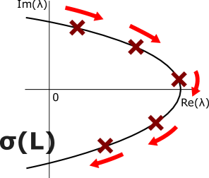
Figure 2.1: Eigenvalues $\lambda$ of $L_{\xi}$ given as maroon $x$’s. As $\xi$ changes, each individual eigenvalue moves holomorphically with its path given in red. (It is artistic license that the paths are unidirectional.) The spectrum of $L$, $\sigma\left(L\right)$, is graphed in black. The union of all of these eigenvalues $\lambda$ forms $\sigma\left(L\right)$.

Proposition 3.

[11, Proposition 3.1] Consider the operator $L$ as in (1.2) acting on $L^{2}\left(\mathbb{R}\right)$ with domain $H^{1}\left(\mathbb{R}\right)$ and the associated Bloch operators $\left\{L_{\xi}\right\}_{\xi\in\left[-\frac{1}{2},\frac{1}{2}\right)}$ acting on $L_{\text{per}}^{2}[0,2\pi)$ with domain $H_{\text{per}}^{1}[0,2\pi)$. Then $\lambda$ is in the $L^{2}\left(\mathbb{R}\right)$ spectrum of $L$ if and only if there exists some $\xi\in\left[-\frac{1}{2},\frac{1}{2}\right)$ so that $\lambda$ is in the $L_{\text{per}}^{2}[0,2\pi)$ spectrum of $L_{\xi}$ with an eigenfunction of the form $e^{i\xi x}v\left(x\right)$ with $v\in H_{\text{per}}^{1}[0,2\pi)$.

As the resolvent of each $L_{\xi}$ with domain $H_{\text{per}}^{1}[0,2\pi)$ is a compact operator, then the spectrum of $L_{\xi}$ is a countable set of isolated eigenvalues with finite multiplicity [6]. Note that from (2.2), $\xi$ appears in $L_{\xi}$ as a polynomial and so $L_{\xi}$ is holomorphic as a function of $\xi$, and thus [13, Theorem 1.7 from VII-§1] given a closed curve $\Gamma$ that separates the spectrum, its corresponding spectral projection is holomorphic in $\xi$ and [13, Theorem 1.8 from VII-§1] any finite system of eigenvalues which depend holomorphically on $\xi$. See Figure 2.1 for a depiction of the spectral picture.

In particular, let $\lambda$ be an eigenvalue of $L_{\xi_{0}}$ and $\Gamma$ be a curve that contains $\lambda$ and no other eigenvalue of $L_{\xi_{0}}$. Then there is some interval $I\subset\left[-\frac{1}{2},\frac{1}{2}\right)$, with $\xi_{0}\in I$, so that the following spectral projection

$$\tilde{P}_{\lambda}\left(\xi\right)=\frac{1}{2\pi i}\int_{\Gamma}R\left(\zeta,L_{\xi}\right)\ d\zeta$$ (2.3)

is holomorphic on $I$, where $R\left(\zeta,L_{\xi}\right)$ is the resolvent of $L_{\xi}$.

The Bloch transform may be used to relate the domain of the Bloch operators $\left\{L_{\xi}\right\}_{\xi\in\left[-\frac{1}{2},\frac{1}{2}\right)}$ to the domain of $L$. To explain the former domain, first fix $\xi$ and consider $g\left(\xi,\cdot\right)\in\mathcal{D}\left(L_{\xi}\right)=H_{\text{per}}^{1}[0,2\pi)$. The Bloch transform requires the map $\xi\in\left[-\frac{1}{2},\frac{1}{2}\right)\mapsto g\left(\xi,\cdot\right)\in H_{\text{per}}^{1}[0,2\pi)$ be $L^{2}\left(\left[-\frac{1}{2},\frac{1}{2}\right);H_{\text{per}}^{1}[0,2\pi)\right)$, identifying this as the domain of the Bloch operators $\left\{L_{\xi}\right\}_{\xi\in\left[-\frac{1}{2},\frac{1}{2}\right)}$ . We define the Bloch transform of $f\in L^{2}\left(\mathbb{R}\right)$ to be the unique function $\check{f}\in L^{2}\left(\left[-\frac{1}{2},\frac{1}{2}\right);L_{\text{per}}^{2}[0,2\pi)\right)$ which satisfies

$$f\left(x\right)=\int_{-1/2}^{1/2}\check{f}\left(\xi,x\right)e^{i\xi x}\ d\xi\,.$$ (2.4)

We have uniqueness because there is an explicit formula for $\check{f}$; starting from the Fourier inversion formula, if we break the integral into blocks of the form $\left[j-1/2,j+1/2\right]$ with $j\in\mathbb{Z}$,

$$f\left(x\right)=\frac{1}{2\pi}\int_{\mathbb{R}}\hat{f}\left(\xi\right)e^{i\xi x}\ d\xi=\int_{-1/2}^{1/2}\left(\sum_{j\in\mathbb{Z}}\hat{f}\left(\xi+j\right)e^{ijx}\right)e^{i\xi x}\ d\xi\,.$$

Then explicitly,

$$\check{f}\left(\xi,x\right)=\sum_{j\in\mathbb{Z}}\hat{f}\left(\xi+j\right)e^{ijx}\,.$$

From Parseval’s theorem we see that the Bloch transform is an isometry,

$$\left\|f\right\|_{L^{2}\left(\mathbb{R}\right)}^{2}=2\pi\int_{-1/2}^{1/2}\left\|\check{f}\left(\xi,\cdot\right)\right\|_{L^{2}\left(\mathbb{R}\backslash 2\pi\mathbb{Z}\right)}^{2}\ d\xi\,.$$ (2.5)

We can also use the Bloch transform to write the linear evolution $e^{Lt}$ in terms of the linear evolution of the Bloch operators [12, Equation 1.15]. Specifically, given an $f_{0}\in L^{2}\left(\mathbb{R}\right),$ we have

$$e^{Lt}f_{0}\left(x\right)=\frac{1}{2\pi}\int_{-1/2}^{1/2}e^{i\xi x}e^{L_{\xi}t}\check{f_{0}}\left(\xi,x\right)\ d\xi\,.$$ (2.6)

2.2 Bloch-Space Projections

Our first goal is to use the unstable spectrum of $L$ to show that the linear part of (1.4) has some sort of exponential growth. We assume that the spectrum of $L$ is unstable, so let $\lambda\in\sigma\left(L\right)\cap\left\{z\in\mathbb{C}\ \middle|\ \text{Re }z>0\right\}$. In Proposition 3 we characterized the $L^{2}\left(\mathbb{R}\right)$ spectrum of $L$ in terms of the $L_{\text{per}}^{2}[0,2\pi)$ eigenvalues of the one-parameter family of Bloch operators $L_{\xi}$: there must be some $\xi_{0}\in\left[-\frac{1}{2},\frac{1}{2}\right)$ so that $\lambda$ is an eigenvalue of $L_{\xi_{0}}$ with eigenfunction $\phi\left(\xi_{0},x\right)$. Note that $\phi$ when considered as an initial perturbation has exponential growth as $e^{L_{\xi_{0}}t}\phi=e^{\lambda t}\phi$, albeit in $L_{\text{per}}^{2}[0,2\pi)$. We use the Bloch Transform (2.4) to extend $\phi$ into some function in $L^{2}\left(\mathbb{R}\right)$ that has exponential growth.

First we extend $\phi\left(\xi,x\right)$ to more $\xi$ values than just $\xi_{0}$. Using the spectral projection around a single eigenvalue of $L_{\xi_{0}},$ $\tilde{P}_{\lambda}\left(\xi\right)$ introduced in (2.3), for $\xi$ in some interval $I$ we may continuously define $\phi\left(\xi,x\right)=\tilde{P}_{\lambda}\left(\xi\right)\phi\left(\xi_{0},x\right)$. We restrict the contour $\Gamma$ and interval $I$ to be sufficiently small so that

$$\beta=\inf\text{Re }\Gamma>0\ ,$$ (2.7)

then we can use the Bloch Transform to define the following function in $L^{2}\left(\mathbb{R}\right)$,

$$f_{0}\left(x\right)=\frac{1}{2\pi}\int_{I}e^{i\xi x}\phi\left(\xi,x\right)\ d\xi\ .$$ (2.8)

As each $\phi\left(\xi,x\right)$ is a linear combination of eigenfunction of $L_{\xi}$ with eigenvalues $\lambda^{\prime}$ that satisfy $\text{Re}\lambda^{\prime}>\beta$, then $\left\|e^{L_{\xi}t}\phi\left(\xi,x\right)\right\|_{L_{\text{per}}^{2}[0,2\pi)}>e^{\beta t}\left\|\phi\left(\xi,x\right)\right\|_{L_{\text{per}}^{2}[0,2\pi)}$. Hence when using (2.5) and (2.6) we have the estimate that

$$\left\|e^{Lt}f_{0}\right\|_{L^{2}\left(\mathbb{R}\right)}^{2} = \frac{1}{2\pi}\int_{I}\left\|e^{\lambda_{i}\left(\xi\right)t}\phi_{i}\left(\xi,\cdot\right)\right\|_{L^{2}\left(\mathbb{R}\backslash 2\pi\mathbb{Z}\right)}^{2}$$

$$\geq \frac{1}{2\pi}e^{\beta t}\inf_{\xi\in I}\left\|\phi_{i}\left(\xi,\cdot\right)\right\|_{L^{2}\left(\mathbb{R}\backslash 2\pi\mathbb{Z}\right)}^{2}\,.$$

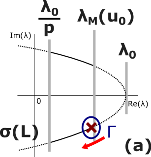
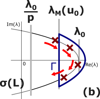
Figure 2.2: The spectrum of $L$, $\sigma\left(L\right)$, with the lines $\text{Re }z=\frac{\lambda_{0}}{p}$, $\text{Re }z=\lambda_{M}\left(u_{0}\right)$, and $\text{Re }z=\lambda_{0}$ shown. (a) The contour $\Gamma$ chosen for $P$ which is chosen close to an eigenvalue $\lambda\left(\xi_{0}\right)$, which in turn is close to $\lambda_{M}$. The interval $I$ is chosen sufficiently small so that no other eigenvalues enter the region enclosed by $\Gamma$. (b) The contour $\Gamma$ chosen for $P^{\prime}$. Note that as $\xi$ varies, eigenvalues may enter or exit the region enclosed by $\Gamma$: Hypothesis 5 claims that this happens finitely many times, so we may consider finitely many $\xi$-intervals $I_{j}$ where the number of eigenvalues (counted by multiplicity) enclosed by $\Gamma$ is a constant.

The intuition behind this is constructing an initial perturbation that is close to the eigenfunction $\phi\left(\xi_{0},x\right)$. In the sequel our strategy changes to instead defining a projection $P$ that recognizes when such “eigenfunctions” are present in an initial perturbation $u_{0}$. This has the advantage of being widely applicable to all initial perturbations rather than just a constructed few.

As a technical issue we require any such “eigenfunctions” to have a sufficient level of exponential growth. To that end we first define the following quantity which will be the maximum rate of exponential growth an initial perturbation $u_{0}$ contains,

$$\lambda_{M}\left(u_{0}\right)=\sup\left\{\text{Re }\lambda\ \middle|\ \tilde{P}_{\lambda}\left(u_{0}\right)^{\vee}\neq 0,\lambda\in\sigma\left(L_{\xi}\right)\text{ for any }\xi\in\left[-\frac{1}{2},\frac{1}{2}\right)\right\}\,,$$ (2.9)

where $\tilde{P}_{\lambda}$ is a spectral projection to the eigenspace of $\lambda$ as defined in equation (2.3). Note that the condition in (2.9) is analogous to requiring “$\lambda\in\sigma\left(L\right)$,” but accounts for the technicality that if $\lambda$ is an eigenvalue for multiple $L_{\xi}$ then $\tilde{P}_{\lambda}$ as defined in (2.3) is not unique.

We will construct this projection $P$ analogously to (2.8): as $\phi\left(\xi_{0},x\right)$ was extended to $\phi\left(\xi,x\right)$ by prepending $\tilde{P}_{\lambda}$, we shall do so here as well. We choose our $\tilde{P}_{\lambda}$ so that $\lambda$ is arbitrarily close to $\lambda_{M}$. That is, let $\epsilon>0$ with $0<\lambda_{M}-\epsilon<\lambda_{M}$. Then choose an eigenvalue $\lambda$ of $L_{\xi_{0}}$ with $\tilde{P}_{\lambda}\left(u_{0}\right)^{\vee}\neq 0$ so that $\lambda_{M}-\text{Re }\lambda<\frac{\epsilon}{2}$, and restrict the contour $\Gamma$ and interval $I$ containing $\xi_{0}$ so that $\lambda_{M}-\inf\ \text{Re }\Gamma<\epsilon$ and $\tilde{P}_{\lambda}\left(\xi\right)$ is holomorphic on $I$. See Figure 2.2 (a) for an illustration. We may then use the Bloch Transform (2.4) to define the following projection,

$$Pu\left(x\right)=\int_{I}e^{i\xi x}\tilde{P}_{\lambda}\left(\xi\right)\check{u}\left(\xi,x\right)\ d\xi\,.$$ (2.10)

To see that $P$ is a projection, first note that by the uniqueness of (2.4) we see that $\left(Pu\right)^{\vee}=\tilde{P}_{\lambda}\check{u}$, and so $P^{2}u=Pu$. Secondly, applying 2.5 and that $\left\|\tilde{P}_{\lambda}\right\|_{L_{\text{per}}^{2}[0,2\pi)}\leq 1$ gives that $\left\|P\right\|_{L^{2}\left(\mathbb{R}\right)}\leq 1$. Furthermore the spectral projection $\tilde{P}_{\lambda}\left(\xi\right)$ commutes with the semigroup $e^{L_{\xi}t}$ for each $\xi$ [19, Theorem 3.14.10], which we can use to show that $P$ commutes with $e^{Lt}$ as well.

Lemma 4.

Suppose $u_{0}$ is an initial perturbation to (1.1). Then there exists some constant $C>0$ depending only on $u_{0}$ so that for any $\omega<\lambda_{M}$ sufficiently close to $\lambda_{M}$ defined in (2.9), we have the linear growth estimate

$$C\delta e^{\omega t}\leq\left\|e^{Lt}\delta u_{0}\right\|_{X}\,.$$

Proof.

As $P$ is a projection, then

$$\left\|Pu\right\|_{X}\leq\left\|u\right\|_{X}\,.$$

So it suffices to show this exponential growth for the projected linear part $Pe^{Lt}\delta u_{0}$. Set $\epsilon=\lambda_{M}-\omega$ and recall the choice of $\lambda$ in (2.10), restricting the interval $I$ so that $\tilde{P}_{\lambda}\left(\xi\right)\left(u_{0}\right)^{\vee}\neq 0$ for all $\xi\in I$. As $\tilde{P}_{\lambda}\left(\xi\right)\left(u_{0}\right)^{\vee}$ is a linear combination of eigenfunctions of $L_{\xi}$ with eigenvalues $\lambda^{\prime}$ that satisfy $\text{Re }\lambda^{\prime}>\omega$, $\left\|e^{L_{\xi}t}\right\|_{L_{\text{per}}^{2}[0,2\pi)}>e^{\omega t}$, and after applying (2.5),

$$\left\|Pe^{Lt}\delta u_{0}\right\|_{X} \geq \int_{I}\left\|e^{L_{\xi}t}\tilde{P}\left(\xi\right)\left(\delta u_{0}\right)^{\vee}\left(\xi,\cdot\right)\ e^{i\xi\cdot}\right\|_{L_{\text{per}}^{2}[0,2\pi)}\ d\xi$$

$$\geq \delta e^{\omega t}\int_{I}\inf_{\xi\in I}\left(\left\|\tilde{P}\left(\xi\right)\left(u_{0}\right)^{\vee}\left(\xi,\cdot\right)\right\|_{L_{\text{per}}^{2}[0,2\pi)}\right)\ d\xi\,.$$

∎

Our instability argument requires that $\lambda_{M}$ be sufficiently large to attain a certain minimum level of exponential growth. To define this level, we first need to determine an upper bound of $\lambda_{M}\left(u_{0}\right)$ over all choices of initial perturbations $u_{0}$,

$$\lambda_{0}=\sup\left\{\text{Re }\lambda\ \middle|\ \lambda\in\sigma\left(L\right)\right\}\,.$$ (2.11)

Note that as $L$ was assumed to be sectorial, then $\lambda_{0}$ is necessarily finite. As part of the upcoming Hypothesis 5 we assume that this quantity is finite. We later determine in Theorem 7 that a sufficient level of exponential growth is attained if $\frac{\lambda_{0}}{p}<\lambda_{M}$, where $p$ is the power of the nonlinearity as in equation (1.3). Put another way, if we define

$$\Sigma_{U}=\sigma\left(L\right)\cap\left\{\text{Re}\left(z\right)>\frac{\lambda_{0}}{p}\ \middle|\ z\in\mathbb{C}\right\}$$

then there is a sufficient amount of exponential growth if for some $\lambda\in\Sigma_{U}$, $\lambda$ an eigenvalue of $L_{\xi_{0}}$, we have that $\tilde{P}_{\lambda}\left(u_{0}\right)^{\vee}\neq 0$. This is what is precisely meant by saying $u_{0}$ “activates” the unstable part of the spectrum. We now make a hypothesis on $\Sigma_{U}$, that eigenvalues do not enter and exit it too many times.

Hypothesis 5.

For each initial perturbation $u_{0}$ of (1.1) with $\frac{\lambda_{0}}{p}<\lambda_{M}\left(u_{0}\right)$, there is a finite partition of $\left[-\frac{1}{2},\frac{1}{2}\right)$ into intervals $I_{j}$ so that the number of eigenvalues of $L_{\xi}$ (defined in (2.2), counted by multiplicity) in

$$A_{u_{0}}=\Sigma_{U}\cap\left\{z\in\mathbb{C}\ \middle|\ \text{Re }z>\lambda_{M}\left(u_{0}\right)\right\}$$

is constant for $\xi\in I_{j}$.

For a visual depiction of this latter assumption, see Figure 2.2 (b), where eigenvalues are allowed to enter and exit a contour $\Gamma$ enclosing only $A_{u_{0}}$ — and no other part of $\sigma\left(L\right)$ — only finitely many times. In [7, Figure 6] [16, Figure 3] a numerical calculation of the point spectrum of $L_{\xi}$ appears to agree with this hypothesis.

As it stands, a naive exponential growth upper bound for $u_{0}$ — that is, obtained solely by looking at the spectrum of $L$ — would be $e^{\lambda_{0}t}$. If we bound the nonlinear part in (1.4) by this exponential function $e^{\lambda_{0}t}$, then it would overshadow the lesser growth $e^{\left(\lambda_{M}-\epsilon\right)t}$ that (2.10) can provide for the linear part. But we can take advantage of the fact that for all $\lambda\in\sigma\left(L\right)$ with $\text{Re }\lambda>\lambda_{M}$, then $\tilde{P}_{\lambda}u_{0}=0$ (for any choice of $\tilde{P}_{\lambda}$). Thus intuitively $u_{0}$ should “ignore” that part of the spectrum, and the exponential growth upper bound should instead be $e^{\lambda_{M}t}$.

Lemma 6.

Suppose that (1.1) satisfies Hypothesis 5 and let $u_{0}$ be an initial perturbation with $\frac{\lambda_{0}}{p}<\lambda_{M}\left(u_{0}\right)$. Then there exists some constant $C>0$ depending only on $u_{0}$ so that we have the linear growth estimate

$$\left\|e^{Lt}\delta u_{0}\right\|_{X}\leq C\delta e^{\lambda_{M}t}\,.$$

Proof.

We start by using Hypothesis 5 to find intervals $I_{j}$ a finite partition of $\left[-\frac{1}{2},\frac{1}{2}\right)$ so that the number of eigenvalues of $L_{\xi}$ (counted by multiplicity) in $A_{u_{0}}$ is constant for each $\xi\in I_{j}$. Let $\Gamma$ be a curve that encloses all of $A_{u_{0}}$ and no other part of $\sigma\left(L\right)$ (see Figure 2.2 (b)). Then we define the following spectral projection,

$$\tilde{P}^{\prime}\left(\xi\right)u=\int_{\Gamma}R\left(\zeta,L_{\xi}\right)\ d\zeta\,.$$

Note that by construction $\left(I-\tilde{P}^{\prime}\left(\xi\right)\right)\left(u_{0}\right)^{\vee}\left(\xi,x\right)=\left(u_{0}\right)^{\vee}\left(\xi,x\right)$. Combining this with (2.6),

$$e^{Lt}u_{0}\left(x\right)=\frac{1}{2\pi}\sum_{j}\int_{I_{j}}e^{i\xi x}e^{L_{\xi}t}\left(I-\tilde{P}^{\prime}\left(\xi\right)\right)\left(u_{0}\right)^{\vee}\left(\xi,x\right)\ d\xi$$

and [19, Theorem 3.14.10] we see that $\tilde{P}^{\prime}$ commutes with $e^{L_{\xi}t}$ and $\left\|\left(I-\tilde{P}^{\prime}\left(\xi\right)\right)e^{L_{\xi}t}\right\|_{L_{\text{per}}^{2}[0,2\pi)}\leq e^{\lambda_{M}t}$. This gives the growth estimate. ∎

3 Nonlinear Instability

We now state our main instability result. With Definition 2 in mind we start by defining $u_{\delta}$, for $\delta>0$, to be the solution to the following evolution equation,

$$\left\{\begin{aligned} \left(u_{\delta}\left(x,t\right)\right)_{t}&=Lu_{\delta}\left(x,t\right)+\mathcal{N}\left(u_{\delta}\left(x,t\right)\right)\\ u_{\delta}\left(x,0\right)&=\delta u_{0}\left(x\right)\,.\end{aligned}\right.$$ (3.1)

Showing that the initial perturbation $u_{0}$ is unstable is equivalent to showing that $u_{\delta}$ cannot be made arbitrarily small by taking $\delta$ arbitrarily small. In our instability theorem we find an explicit time $T$ where the solution fails to be arbitrarily small.

Theorem 7.

Consider the initial value problem (1.1), with $L$ a sectorial operator with $2\pi$-periodic coefficients as defined in (1.2), and $\mathcal{N}$ a nonlinear operator satisfying the polynomial estimate (1.3). Assume that Hypothesis 5 holds and let $u_{0}$ be an initial perturbation with $\lambda_{M}\left(u_{0}\right)>\lambda_{0}/p$. Then $u_{0}$ is unstable in the sense of Definition 2 as there exist $\epsilon>0$ and $\eta>0$ sufficiently small so that for all $\delta<\eta$, at the time $T$ when

$$e^{\lambda_{M}\left(u_{0}\right)T}=\frac{2\eta}{\delta}\,,$$ (3.2)

we have

$$\left\|u_{\delta}\left(\cdot,T\right)\right\|_{L^{2}\left(\mathbb{R}\right)}>\epsilon\,,$$

where $\lambda_{M}\left(u_{0}\right)$ is given in equation (2.9), $\lambda_{0}$ is given in equation (2.11), and $p$ is given in equation (1.3).

Recall from the introduction that our general strategy was to use (1.5) to pit the exponential growth of the linear term obtained from the unstable spectrum of $L$ against the nonlinear term’s slower growth. The former was developed in Lemmas 4 and 6, so we handle the latter below.

Lemma 8.

For $u_{0},u_{\delta},T,\lambda_{M}\left(u_{0}\right),\lambda_{0},p$ as in Theorem 7, then if $\lambda_{M}\left(u_{0}\right)>\lambda_{0}/p$ we have

$$\left\|u_{\delta}\left(\cdot,t\right)\right\|_{X}\leq\delta Ce^{\lambda_{M}\left(u_{0}\right)t}\qquad\text{for }t\leq T\,.$$

Proof.

For $t\leq T$ we define the quantity

$$\rho\left(t\right)=\sup_{0\leq s\leq t}\left\|u_{\delta}\left(s\right)\right\|_{X}e^{-\lambda_{M}s}\>.$$ (3.3)

To prove the result, it is sufficient to show that $\rho\left(t\right)$ is uniformly bounded for $t\leq T$. We start by taking the norm of (1.4). From Lemma 6 we have that $\left\|e^{Lt}\delta u_{0}\right\|_{X}\leq\delta Ce^{\lambda_{M}t}$, and as $L$ is sectorial then $\left\|e^{Lt}\right\|_{X}\leq e^{\lambda_{0}t}$. Then after recalling (1.3), we have

$$\left\|u_{\delta}\left(\cdot,t\right)\right\|_{X}\leq\delta Ce^{\lambda_{M}t}+\int_{0}^{t}e^{\lambda_{0}\left(t-s\right)}\left\|u_{\delta}\left(\cdot,s\right)\right\|_{X}^{p}\ ds\,.$$

Then we multiply and divide the nonlinear term by $e^{-p\lambda_{M}s}$, apply (3.3), evaluate the integral, and note that $\rho\left(t\right)$ is monotone increasing to obtain

$$\left\|u_{\delta}\left(\cdot,t\right)\right\|_{X}\leq\delta Ce^{\lambda_{M}t}+\rho\left(t\right)^{p}\frac{e^{p\lambda_{M}t}-e^{\lambda_{0}t}}{p\lambda_{M}-\lambda_{0}}\,.$$ (3.4)

Recall the hypothesis $\lambda_{0}/p<\lambda_{M}$, and note that it implies

$$e^{\lambda_{0}t}<e^{p\lambda_{M}t}\quad\text{and}\quad 0<p\lambda_{M}-\lambda_{0}\,,$$

so we may focus solely on the larger exponential growth.

Note that this upper bound (3.4) also applies for all $\left\|u_{\delta}\left(\cdot,s\right)\right\|_{X}$ for $s\leq t$. Multiplying both sides by $e^{-\lambda_{M}s}$ and taking the supremum over all $s\leq t$ yields

$$\rho\left(t\right)\leq\delta C+\rho\left(t\right)^{p}\frac{e^{\left(p-1\right)\lambda_{M}t}}{p\lambda_{M}-\lambda_{0}}\,.$$ (3.5)

Replacing the right hand side exponential term’s $t$ with $T$, recalling (3.2), and dividing both sides by $\delta$,

$$\frac{\rho\left(t\right)}{\delta}\leq C+\frac{\left(2\eta\right)^{p-1}}{p\lambda_{M}-\lambda_{0}}\left(\frac{\rho\left(t\right)}{\delta}\right)^{p}\,.$$

Setting $z=\frac{\rho\left(t\right)}{\delta}$ leads to the equivalent polynomial inequality valid for $t\leq T$,

$$0\leq C-z+\frac{\left(2\eta\right)^{p-1}}{p\lambda_{M}-\lambda_{0}}z^{p}\,.$$ (3.6)

This polynomial has a critical point at

$$z=\frac{1}{2\eta}\left(\frac{p\lambda_{M}-\lambda_{0}}{p}\right)^{\frac{1}{p-1}}>0\,.$$

And at this critical point the polynomial takes on the value

$$C-\frac{1}{2\eta}\left[\left(\frac{p\lambda_{M}-\lambda_{0}}{p}\right)^{\frac{1}{p-1}}\left(1+\frac{1}{p}\right)\right]\,.$$

Then so long as $\eta$ is smaller than some expression that only involves $p,\lambda_{M},\lambda_{0}$, then the polynomial will be negative at some $z$-value to the right of $z=0$. In particular, it will have a root to the right of $z=0$.

When $t=0$, $z=\frac{\left\|u_{\delta}\left(0\right)\right\|}{\delta}=1$, so choosing $\eta$ sufficiently small will satisfy the polynomial inequality initially at $t=0$. Then the existence of a root means that $z$ is uniformly bounded for $t\leq T$, and hence the uniform bound for $\rho$ for $t\leq T$. ∎

Now we can use this lemma to establish an upper bound for the nonlinear growth in (1.4) and finally prove Theorem 7.

Proof.

(Of Theorem 7)

Lemma 4, when $t=T$, gives us that

$$C\eta\leq\left\|e^{LT}\delta u_{0}\right\|_{X}\,.$$ (3.7)

From Lemma 8, we can bound the nonlinear part of $u_{\delta}$ by

$$\left\|\int_{0}^{t}e^{L\left(t-s\right)}\mathcal{N}\left(u_{\delta}\left(s\right)\right)\ ds\right\|_{X} \leq \left(C\delta e^{\lambda_{M}t}\right)^{p}\int_{0}^{t}e^{\lambda_{M}\left(t-s\right)}\ ds\,.$$

In particular, when $t=T$, we have

$$\left\|\int_{0}^{T}e^{L\left(T-s\right)}\mathcal{N}\left(u_{\delta}\left(s\right)\right)\ ds\right\|_{X}\leq\bar{C}\eta^{p}\,.$$ (3.8)

Then if $\eta$ is chosen sufficiently small so that $C\eta\geq\bar{C}\eta^{p}$, then by the reverse triangle inequality we have

$$0<C\eta-\bar{C}\eta^{p}\leq\left|\left\|e^{LT}\delta u_{0}\right\|_{X}-\left\|\int_{0}^{T}e^{L\left(T-s\right)}\mathcal{N}\left(u_{\delta}\right)\right\|_{X}\right|\leq\left\|u_{\delta}\left(T\right)\right\|\,.$$

Note that the leftmost term $C\eta-\bar{C}\eta^{p}$ is a positive constant independent of $\delta$: this becomes our $\epsilon$, which completes the proof. ∎

4 Extension to Dissipative Systems of Conservation Laws

Recall that our main Theorem 7 was proven in the context of reaction-diffusion type systems of the form (1.1): specifically for systems with no derivatives in the nonlinearity. Some examples of such systems would be scalar reaction diffusion, FitzHugh-Nagumo [14], the Klausmeier model for vegetation stripe formulation [18, 17], and the Belousov-Zhabotinskii reaction [4]. However, our general methodology is sufficiently robust enough that it can apply more widely to dissipative systems of conservation laws. As a specific example, consider the following Korteweg-de-Vries/Kuramoto-Sivashinsky (KdV-KS) equation

$$p_{t}+pp_{x}+p_{xxx}+\beta\left(p_{xx}+p_{xxxx}\right)=0$$ (4.1)

with $0<\beta\ll 1$, which arises in the context of inclined thin film flow [10]. It was shown in [1, 10] that this equation admits periodic traveling wave solutions $\phi$ whose linearization satisfies Hypothesis 5. If we consider solutions of the form $p\left(x,t\right)=\phi\left(x\right)+u\left(x,t\right)$, we find that $u$ satisfies the following perturbation equation [3, Lemma 3.3]

$$u_{t}+u_{xxx}+\beta\left(u_{xx}+u_{xxxx}\right)+\phi u_{x}+\phi^{\prime}u+uu_{x}=0\,.$$ (4.2)

Our goal is to characterize which initial perturbations $u_{0}$ of our traveling wave $\phi$ will result in an unstable solution $p$. Note that the nonlinearity $uu_{x}$ does not in any standard Sobolev space satisfy a polynomial estimate of the form (1.3). Nevertheless we can use the following damping estimate as in [3, Proposition 3.4] to obtain a workable analogue. For completeness we reproduce the proof of this damping estimate.

Lemma 9.

Let $u$ be a solution to (4.2). Then $u$ satisfies the following nonlinear damping estimate

$$\left\|u\right\|_{H^{2}}\leq e^{-\beta t}\left\|u\left(0\right)\right\|_{H^{2}}+C\int_{0}^{T}e^{-\beta\left(t-s\right)}\left\|u\left(s\right)\right\|_{H^{1}\left(\mathbb{R}\right)}\ ds$$ (4.3)

for some constant $C>0$.

Proof.

Let $\left\langle\cdot,\cdot\right\rangle$ denote the $L^{2}\left(\mathbb{R}\right)$ inner product. Using integration by parts,

$$\frac{1}{2}\frac{d}{dt}\left(\left\|u\right\|_{H^{2}\left(\mathbb{R}\right)}^{2}\right)=\left\langle u_{t},u-u_{xx}+u_{xxxx}\right\rangle\,.$$ (4.4)

We can obtain $u_{t}$ from (4.2). Using Cauchy-Schwartz, Young’s inequality, and the fact that $\left\|u\right\|_{L^{\infty}\left(\mathbb{R}\right)}\leq\left\|u\right\|_{H^{1}\left(\mathbb{R}\right)}$ allows us to bound the nonlinear term,

$$\left\langle uu_{x},u_{xxxx}-u_{xx}\right\rangle\leq\frac{1}{2}\left\|u\right\|_{L^{\infty}\left(\mathbb{R}\right)}\left(\left(1+\frac{1}{2\beta}\left\|u\right\|_{L^{\infty}\left(\mathbb{R}\right)}\right)\left\|u_{x}\right\|_{L^{2}\left(\mathbb{R}\right)}^{2}+\left\|u_{xx}\right\|_{L^{2}\left(\mathbb{R}\right)}^{2}\right)+\frac{\beta}{2}\left\|u_{xxxx}\right\|_{L^{2}\left(\mathbb{R}\right)}\,.$$

The remainder of (4.4) can be handled with integration by parts and recognizing perfect derivatives, resulting in the bound

$$\frac{1}{2}\frac{d}{dt}\left(\left\|u\right\|_{H^{2}\left(\mathbb{R}\right)}^{2}\right)\leq\sum_{j=0}^{3}\alpha_{j}\left\|\partial_{x}^{j}u\right\|_{L^{2}\left(\mathbb{R}\right)}^{2}-\frac{\beta}{2}\left\|u_{xxxx}\right\|_{L^{2}\left(\mathbb{R}\right)}^{2}\,,$$ (4.5)

where the $\alpha_{j}$ are non-negative constants depending on $\delta$, $\left\|\partial_{x}^{k}\phi\right\|_{L^{\infty}}$ for $k=0,1,2,3,4$, and $\left\|u\right\|_{L^{\infty}}$.

Before proceeding we derive a useful Sobolev interpolation inequality. Using integration by parts, for integer $j\geq 1$ we have

$$\left\|\partial_{x}^{j}u\right\|_{L^{2}\left(\mathbb{R}\right)}^{2}=-\left\langle\partial_{x}^{j-1}u,\partial_{x}^{j+1}u\right\rangle\,.$$

Using Cauchy-Schwartz and Young’s inequality with an arbitrary positive constant $a_{j}$ yields the inequality

$$\left\|\partial_{x}^{j}u\right\|_{L^{2}\left(\mathbb{R}\right)}^{2}\leq\frac{1}{4a_{j}}\left\|\partial_{x}^{j-1}\right\|_{L^{2}\left(\mathbb{R}\right)}^{2}+a_{j}\left\|\partial_{x}^{j+1}u\right\|_{L^{2}\left(\mathbb{R}\right)}^{2}\,.$$

Taking a linear combination of the $j=2,3$ cases, for appropriate choices of the $a_{j}$ and a sufficiently large constant $\tilde{C}>0$, we can obtain the following Sobolev interpolation inequality

$$\left(\alpha_{2}+\frac{\beta}{2}\right)\left\|u_{xx}\right\|_{L^{2}\left(\mathbb{R}\right)}^{2}+\alpha_{3}\left\|u_{xxx}\right\|_{L^{2}\left(\mathbb{R}\right)}^{2}\leq\tilde{C}\left\|u_{x}\right\|_{L^{2}\left(\mathbb{R}\right)}^{2}+\frac{\beta}{2}\left\|u_{xxxx}\right\|_{L^{2}\left(\mathbb{R}\right)}^{2}\,.$$ (4.6)

Combining (4.6) and (4.5) gives, for some constant $C>0$,

$$\frac{1}{2}\frac{d}{dt}\left(\left\|u\right\|_{H^{2}\left(\mathbb{R}\right)}^{2}\right)\leq-\frac{\beta}{2}\left\|u\right\|_{H^{2}\left(\mathbb{R}\right)}^{2}+C\left\|u\right\|_{H^{1}\left(\mathbb{R}\right)}^{2}\,.$$

The estimate (4.3) then follows from Gronwall’s inequality. ∎

The key ingredient to the damping estimate was that the leading term $-\beta u_{xxxx}$ of (4.2) was negative: such an estimate is not necessarily limited to the specific PDE (4.1). In particular a damping estimate also holds for the St. Venant equation [15, Proposition 4.2], which is a hyperbolic-parabolic system of balance laws. In light of this, we introduce a general requirement on the nonlinearity, that for constants $\theta>0$, $C>0$, $T>0$, $n\geq 2$, $p>1$, and $t<T$,

$$\left\|\mathcal{N}\left(u\left(t\right)\right)\right\|_{H^{n}\left(\mathbb{R}\right)}\leq\left\|u\left(t\right)\right\|_{H^{1}\left(\mathbb{R}\right)}^{p-1}\left(e^{-\theta t}\left\|u\left(0\right)\right\|_{H^{n}\left(\mathbb{R}\right)}+C\int_{0}^{T}e^{-\theta\left(t-s\right)}\left\|u\left(s\right)\right\|_{H^{1}\left(\mathbb{R}\right)}\ ds\right)\,.$$ (4.7)

We can then prove an alternate instability result.

Theorem 10.

Consider the initial value problem (1.1), with $L$ a sectorial operator with $2\pi$-periodic coefficients as defined in (1.2), and $\mathcal{N}$ a nonlinear operator instead satisfying the estimate (4.7). Assume that Hypothesis 5 holds and let $u_{0}$ be an initial perturbation which satisfies both $\frac{\lambda_{0}+\theta}{p-1}<\lambda_{M}\left(u_{0}\right)$ and $\frac{\lambda_{0}}{p}<\lambda_{M}\left(u_{0}\right)$, then $u_{0}$ is unstable in the sense of Definition 2 as there exist $\epsilon>0$ and $\eta>0$ sufficiently small so that for all $\delta<\eta$, at the time $T$ when

$$e^{\lambda_{M}\left(u_{0}\right)T}=\frac{2\eta}{\delta}\,,$$ (4.8)

we have

$$\left\|u_{\delta}\left(\cdot,T\right)\right\|_{L^{2}\left(\mathbb{R}\right)}>\epsilon\,,$$

where $\lambda_{M}\left(u_{0}\right)$ is given in equation (2.9), $\lambda_{0}$ is given in equation (2.11), and $u_{\delta}$ is the solution to (3.1).

Remark 11.

In Lemma 9 we show that (4.2) satisfies a nonlinear estimate of the form (4.7) with $\theta=\beta$. However, equation (4.6) of the proof can be modified to obtain any $0<\theta<\beta$, so the $\theta$ in the requirement that $\frac{\lambda_{0}+\theta}{p-1}<\lambda_{M}$ is not restrictive.

Proof.

Here we take $X=H^{1}\left(\mathbb{R}\right)$. Lemmas 4 and 6 and the proof of Theorem 7 apply with no further modification, provided we can establish an estimate as in Lemma 8.

We again define $\rho$ as in (3.3) and start by concentrating on the nonlinear term of (1.4). By the triangle inequality and (4.7),

$$\int_{0}^{t}\left\|e^{L\left(t-s\right)}\right\|_{X}\left\|\mathcal{N}\left(u\left(s\right)\right)\right\|_{X}\ ds \leq \int_{0}^{t}e^{\lambda_{0}\left(t-s\right)}\left\|u\left(s\right)\right\|_{X}^{p-1}e^{-\theta s}\left\|u\left(0\right)\right\|_{H^{n}\left(\mathbb{R}\right)}\ ds$$

$$+C\int_{0}^{t}e^{\lambda_{0}\left(t-s\right)}\left\|u\left(s\right)\right\|_{X}^{p-1}\int_{0}^{s}e^{-\theta\left(s-s^{\prime}\right)}\left\|u\left(s^{\prime}\right)\right\|_{X}\ ds^{\prime}\ ds\,.$$

We multiply and divide by appropriate powers of $e^{\lambda_{M}s}$, bound by $\rho$, and evaluate the integrals to obtain the analogue of (3.4),

$$\left\|u_{\delta}\left(t\right)\right\|_{X} \leq \delta Ce^{\lambda_{M}t}+\rho^{p-1}\left(t\right)\left\|u_{\delta}\left(0\right)\right\|_{H^{n}}\frac{e^{\left(\left(p-1\right)\lambda_{M}-\theta\right)t}-e^{\lambda_{0}t}}{\left(p-1\right)\lambda_{M}-\left(\theta+\lambda_{0}\right)}$$

$$+\left(\frac{C\rho^{p}\left(t\right)}{\theta+\lambda_{M}}\right)\left(\frac{e^{p\lambda_{M}t}-e^{\lambda_{0}t}}{p\lambda_{M}-\lambda_{0}}-\frac{e^{\left(\left(p-1\right)\lambda_{M}-\theta\right)t}-e^{\lambda_{0}t}}{\left(p-1\right)\lambda_{M}-\left(\theta+\lambda_{0}\right)}\right)\,.$$

Note that the hypotheses $\frac{\lambda_{0}+\theta}{p-1}<\lambda_{M}$ and $\frac{\lambda_{0}}{p}<\lambda_{M}$ imply that

$$e^{\lambda_{0}t}<e^{\left(\left(p-1\right)\lambda_{M}-\theta\right)t}\quad\text{and}\quad e^{\lambda_{0}t}<e^{p\lambda_{M}t}\,,$$

so we may focus solely on the larger exponential growth.

The upper bound in (4) also applies for all $\left\|u_{\delta}\left(s\right)\right\|_{X}$ for $s\leq t$. Then after multiplying both sides of the inequality by $e^{-\lambda_{M}t}$ and taking the supremum over all $s\leq t$, we have the analogue of (3.5),

$$\rho\left(t\right)\leq\delta C+a_{p-1}\,\rho^{p-1}\left(t\right)e^{\left(p-2\right)\lambda_{M}t}+a_{p}\,\rho^{p}\left(t\right)e^{\left(p-1\right)\lambda_{M}t}\,,$$

where $a_{p-1}$ and $a_{p}$ depend only on $C$, $p$, $\lambda_{0}$, $\lambda_{M}$, $\theta$, and $\left\|u_{\delta}\left(0\right)\right\|_{H^{n}}$.

Replacing the right hand side exponential terms’ $t$ with $T$, recalling (4.8), dividing both sides by $\delta$ and setting $z=\frac{\rho\left(t\right)}{\delta}$, then we have the analogue of (3.6),

$$0\leq a_{p}\,\eta^{p-1}z^{p}+a_{p-1}\,\eta^{p-2}\delta\,z^{p-1}-z+C\,.$$ (4.10)

To find a zero of this polynomial, we compare it with the linear function $C-z$. In particular, on the interval $\left[0,L\right]$ we have

$$\left|\left(a_{p}\,\eta^{p-1}z^{p}+a_{p-1}\,\eta^{p-2}\delta\,z^{p-1}-z+C\right)-\left(C-z\right)\right|\leq a_{p}\,\eta^{p-1}L^{p}+a_{p-1}\,\eta^{p-2}\delta\,L^{p-1}\,.$$

Choosing $L=C+1$ has the function $C-z$ taking on the value $-1$ when $z=L$, and taking $\eta$ sufficiently small ensures that the polynomial (4.10) takes on a negative value when $z=L$. As that same polynomial takes on the positive value $C$ when $z=0$, then it has a zero. As a consequence, then $\rho$ is uniformly bounded. ∎

References

- [1] Blake Barker. Numerical proof of stability of roll waves in the small-amplitude limit for inclined thin film flow. Journal of Differential Equations, 257(8):2950–2983, October 2014.
- [2] Blake Barker, Mathew A. Johnson, Pascal Noble, L. Miguel Rodrigues, and Kevin Zumbrun. Whitham averaged equations and modulational stability of periodic traveling waves of a hyperbolic-parabolic balance law. Journes Equations aux dérivées partielles, pages 1–24, 2010.
- [3] Blake Barker, Mathew A. Johnson, Pascal Noble, L. Miguel Rodrigues, and Kevin Zumbrun. Nonlinear modulational stability of periodic traveling-wave solutions of the generalized Kuramoto-Sivashinsky equation. Physica D: Nonlinear Phenomena, 258:11–46, September 2013.
- [4] Grigory Bordyugov, Nils Fischer, Harald Engel, Niklas Manz, and Oliver Steinbock. Anomalous dispersion in the Belousov-Zhabotinsky reaction: Experiments and modeling. Physica D: Nonlinear Phenomena, 239(11):766–775, June 2010.
- [5] Carmen Chicone. Ordinary differential equations with applications, volume 34. Springer Science & Business Media, 2006.
- [6] Lawrence C. Evans. Partial Differential Equations. Volume 19 of Graduate studies in mathematics. American Mathematical Society, second edition, 1998.
- [7] M. Osman Gani and Toshiyuki Ogawa. Instability of periodic traveling wave solutions in a modified FitzHugh-Nagumo model for excitable media. Applied Mathematics and Computation, 256:968–984, April 2015.
- [8] Dan Henry. Geometric theory of semilinear parabolic equations. Number 840 in Lecture notes in mathematics. Springer, Berlin, 3. printing edition, 1993. OCLC: 257019414.
- [9] Jiayin Jin, Shasha Liao, and Zhiwu Lin. Nonlinear Modulational Instability of Dispersive PDE Models. Arch. Ration. Mech. Anal., 231:1487–1530, 2019.
- [10] Mathew Johnson, Pascal Noble, L. Rodrigues, and Kevin Zumbrun. Spectral stability of periodic wave trains of the Korteweg-de Vries/Kuramoto-Sivashinsky equation in the Korteweg-de Vries limit. Transactions of the American Mathematical Society, 367(3):2159–2212, 2015.
- [11] Mathew A. Johnson. Stability of Small Periodic Waves in Fractional KdV-Type Equations. SIAM Journal on Mathematical Analysis, 45(5):3168–3193, January 2013.
- [12] Mathew A. Johnson and Kevin Zumbrun. Nonlinear stability of periodic traveling wave solutions of systems of viscous conservation laws in the generic case. Journal of Differential Equations, 249(5):1213–1240, September 2010.
- [13] Tosio Kato. Perturbation theory for linear operators. Classics in mathematics. Springer-Verlag, Berlin, 1995.
- [14] Jens D.M. Rademacher, Björn Sandstede, and Arnd Scheel. Computing absolute and essential spectra using continuation. Physica D: Nonlinear Phenomena, 229(2):166–183, May 2007.
- [15] L. Miguel Rodrigues and Kevin Zumbrun. Periodic-Coefficient Damping Estimates, and Stability of Large-Amplitude Roll Waves in Inclined Thin Film Flow. SIAM Journal on Mathematical Analysis, 48(1):268–280, January 2016.
- [16] Jonathan A. Sherratt. Numerical continuation methods for studying periodic travelling wave (wavetrain) solutions of partial differential equations. Applied Mathematics and Computation, 218(9):4684–4694, January 2012.
- [17] Jonathan A. Sherratt. Numerical continuation of boundaries in parameter space between stable and unstable periodic travelling wave (wavetrain) solutions of partial differential equations. Advances in Computational Mathematics, 39(1):175–192, July 2013.
- [18] Jonathan A. Sherratt and Gabriel J. Lord. Nonlinear dynamics and pattern bifurcations in a model for vegetation stripes in semi-arid environments. Theoretical Population Biology, 71(1):1–11, February 2007.
- [19] Olof Staffans. Well-Posed Linear Systems. Number 103 in Encyclopedia of Mathematics and its Applications. Cambridge University Press, Cambridge, 2005.