Secure Trajectory Planning Against
Undetectable Spoofing Attacks

Abstract

This paper studies, for the first time, the trajectory planning problem in adversarial environments, where the objective is to design the trajectory of a robot to reach a desired final state despite the unknown and arbitrary action of an attacker. In particular, we consider a robot moving in a two-dimensional space and equipped with two sensors, namely, a Global Navigation Satellite System (GNSS) sensor and a Radio Signal Strength Indicator (RSSI) sensor. The attacker can arbitrarily spoof the readings of the GNSS sensor and the robot control input so as to maximally deviate its trajectory from the nominal precomputed path. We derive explicit and constructive conditions for the existence of undetectable attacks, through which the attacker deviates the robot trajectory in a stealthy way. Conversely, we characterize the existence of secure trajectories, which guarantee that the robot either moves along the nominal trajectory or that the attack remains detectable. We show that secure trajectories can only exist between a subset of states, and provide a numerical mechanism to compute them. We illustrate our findings through several numerical studies, and discuss that our methods are applicable to different models of robot dynamics, including unicycles. More generally, our results show how control design affects security in systems with nonlinear dynamics.

1 Introduction

Autonomous robots have rapidly been adopted in a broad range of applications, including delivery, exploration, surveillance, and search and rescue. Autonomous robots rely on sensory data to make decisions, plan their trajectories, and apply controls. Yet, as demonstrated by recent studies and real world incidents, sensory data can be accidentally and maliciously compromised, thus undermining the effectiveness of autonomous operations in critical and adversarial applications.

Despite recent advances in understanding and enhancing the security of cyber-physical systems, security tools for autonomous systems are still of limited applicability and effectiveness. In this paper we formulate and solve a secure trajectory planning problem, where the objective is to design the trajectory of a robot to reach a desired final state despite unknown and arbitrary attacks. We consider a robot equipped with a Global Navigation Satellite System (GNSS) sensor and a Radio Signal Strength Indicator (RSSI) sensor, and focus on attackers capable of simultaneously spoofing the GNSS readings and sending falsified control inputs to the robot. We show how the attacker can generate undetectable attacks that maximally deviate the robot from the nominal and precomputed path, and study how the trajectory planner can exploit the RSSI readings to reveal certain attacks. Moreover, we demonstrate the existence of secure trajectories between certain initial and final configurations, and propose a technique to determine the corresponding control inputs. We remark that, because of the nonlinearity of RSSI sensor readings, existing security methods based on linear models are inapplicable in our setting. In fact, our results show for the first time that the security of a system with nonlinear dynamics can be improved by appropriately designing its control inputs.

Related work Security of cyber-physical systems is, by now, a widely studied topic across the controls and computer science communities, among others. Yet, most methods are applicable to static systems or systems with linear dynamics [1, 2, 3, 4, 5], and theoretical results and tools for the security of systems with nonlinear dynamics are still critically lacking. Few exceptions are [6], which considers the problem of controlling a system under attack in a game-theoretic framework, [7], which focuses on nonlinear systems satisfying differential flatness properties, and the recent articles [8, 9], which are however restricted to state the estimation problem in the presence of attacks modifying the system measurements only. Instead, in this work we focus on characterizing detectability of attacks modifying both the measurements and the input of the system, on quantifying their effects on the trajectories, and on the problem of designing nominal control inputs to restrict or prevent undetectable attacks.

The literature on GNSS spoofing attack mechanisms and their detection is also related to this paper. Existing approaches to identify and prevent spoofing attacks can be divided into two categories: filtering-based and redundancy-based techniques. Filtering-based detection techniques rely on signal processing methods to reveal compromised streams of sensory data (e.g., see [10, 11]). Redundancy-based techniques, instead, rely on the availability of measurement from multiple types of sensors to reveal inconsistency in the data (e.g., see [12, 13, 14, 15, 16, 17]). The methods developed in this work combine these two principles. In fact, detection is achieved by processing the sensory data over time, thus ensuring compatibility between the measurements and the robot dynamical model, and by processing the measurements of two or more sensors, thus exploiting redundancy across the two channels.

Paper contribution This paper features four main contributions. First, we demonstrate the existence and characterize the form of undetectable attacks, that is, coordinated attack inputs that deviate the robot trajectory from the nominal path and cannot be detected using the GNSS and RSSI readings. Second, we demonstrate how an attacker can design optimal undetectable attacks that maximally deviate the robot from its nominal path while maintaining undetectability. Third, we show the existence of secure trajectories where, independently of the intensity of the attack, the robot either follows the nominal precomputed path or readily detects the attack. Fourth, we formulate and solve the secure trajectory planning problem, which asks for the design of open-loop control inputs that allow the robot to securely navigate from a given initial configuration to a certain final position. As a minor contribution, we study and characterize undetectable attacks and secure trajectories for robots with unicycle dynamics, thus showing that our techniques are in fact applicable to different nonlinear dynamical robot models and sensors. More generally, our results show that secure trajectories can be substantially different from minimum-time trajectories, and thus demonstrate that the security of a system with nonlinear dynamics depends upon the inputs to the system adopted for control.

Paper organization The remainder of the paper is organized as follows. Section 2 presents our problem setup and attack model. Section 3 contains our notion of undetectability and our characterization of undetectable attacks. Section 4 and Section 5 contain, respectively, the design of optimal undetectable attacks and of secure trajectories. Finally, Section 6 contains an extension of our results to the case of robots with unicycle dynamics, and Section 7 concludes the paper.

2 Problem setup and preliminary notions

We consider a robot with double-integrator dynamics,

$$\underbrace{\begin{bmatrix}{\dot{p}}_{\textup{n}}\\ {\dot{v}}_{\textup{n}}\end{bmatrix}}_{{\dot{x}}_{\textup{n}}}=\underbrace{\begin{bmatrix}\boldsymbol{0}_{2}&I_{2}\\ \boldsymbol{0}_{2}&\boldsymbol{0}_{2}\end{bmatrix}}_{A}\underbrace{\begin{bmatrix}{p}_{\textup{n}}\\ {v}_{\textup{n}}\end{bmatrix}}_{{x}_{\textup{n}}}+\underbrace{\begin{bmatrix}\boldsymbol{0}_{2}\\ I_{2}\end{bmatrix}}_{B}{u}_{\textup{n}},$$ (1)

where ${p}_{\textup{n}}:\mathbb{R}_{\geq 0}\rightarrow{}^{2}$ denotes the robot position, ${v}_{\textup{n}}:\mathbb{R}_{\geq 0}\rightarrow{}^{2}$ the robot velocity, and ${u}_{\textup{n}}:\mathbb{R}_{\geq 0}\rightarrow{}^{2}$ the nominal control input that actuates the acceleration of the robot. The control input ${u}_{\textup{n}}$ is the design parameter that is used to plan the nominal robot trajectory between two desired configurations. We assume that ${u}_{\textup{n}}$ is piecewise continuous, and that

$$\|u_{\text{n}}\|\leq{u}_{\textup{max}},$$

where ${u}_{\textup{max}}\in{}_{>0}$. We let the robot be equipped with two noiseless sensors: a GNSS receiver that provides an absolute measure of the position, and a RSSI sensor that provides a measure of the relative distance between the robot and a base station located at the origin of the reference frame. Specifically, the sensor readings are

$${y}^{\textup{GNSS}}_{\text{n}}={p}_{\textup{n}},\quad\text{and}\quad{y}^{\textup{RSSI}}_{\text{n}}={p}_{\textup{n}}^{\mathsf{T}}{p}_{\textup{n}}.$$ (2)

Although our results can be extended to include different sensors, we focus on GNSS and RSSI sensors because they are available in many practical applications [18].

We consider scenarios where the robot operates in an adversarial environment, where adversaries can simultaneously (i) spoof the GNSS signal ${y}^{\textup{GNSS}}_{\text{n}}$, and (ii) compromise the control input $u_{\text{n}}$. The robot dynamics in the presence of attacks are

$$\underbrace{\begin{bmatrix}\dot{p}\\ \dot{v}\end{bmatrix}}_{\dot{x}}=\underbrace{\begin{bmatrix}\boldsymbol{0}_{2}&I_{2}\\ \boldsymbol{0}_{2}&\boldsymbol{0}_{2}\end{bmatrix}}_{A}\underbrace{\begin{bmatrix}p\\ v\end{bmatrix}}_{x}+\underbrace{\begin{bmatrix}\boldsymbol{0}_{2}\\ I_{2}\end{bmatrix}}_{B}u,$$ (3)

where $u\in{}^{2}$ denotes the attacked control input that obeys the bound on the maximum acceleration $\|u\|\leq u_{\text{max}}$, and

$$y^{\text{GNSS}}=p+{u}^{\textup{GNSS}},\quad\text{and}\quad y^{\text{RSSI}}=p^{\mathsf{T}}p,$$ (4)

where ${u}^{\textup{GNSS}}:\mathbb{R}_{\geq 0}\rightarrow{}^{2}$ denotes the GNSS spoofing signal. Finally, we make the practical assumption that, at time $t=0$, the nominal and attacked configurations satisfy ${x}_{\textup{n}}(0)=x(0)$.

In the remainder of this paper, we will denote the state by $x=[p^{\mathsf{T}},v^{\mathsf{T}}]^{\mathsf{T}}$ or $p$ and $v$ interchangeably, depending on the context. In particular, we let $x=[x_{1},x_{2},x_{3},x_{4}]^{\mathsf{T}}$, and $p=[p^{x},p^{y}]^{\mathsf{T}}=[x_{1},x_{2}]^{\mathsf{T}}$, $v=[v^{x},v^{y}]^{\mathsf{T}}=[x_{3},x_{4}]^{\mathsf{T}}$.

Remark 1.

(Spoofing attack mechanism) Well-known vulnerabilities of GNSS are conventionally associated with the lack of appropriate encryption in the signals that are broadcast by the satellite system. A typical framework to cast spoofing attacks consists in a receiver-spoofer antenna [19] that is capable of sensing the authentic GNSS signals and of rebroadcasting falsified streams of information at a higher signal intensity. The retransmitted signals are typically designed in a way to induce the GNSS receiver to resynchronize with the spoofed information, for instance by gradually increasing the intensity of the retransmission. Once the onboard receiver has resynchronized with the falsified signals, an attacker can arbitrarily decide the GNSS data received by the robot, resulting in (4). A more in-depth discussion of common spoofing schemes and the required hardware can be found in e.g. [19, 20].

In common mobile robotic applications, robots communicate wirelessly with a ground control station, that is responsible to compute the actions and control inputs to be executed by the robot. The use of wireless communication constitutes a possible vulnerability that can be modeled as in (3). See [21] for a discussion of common vulnerabilities of wireless communication in commercial Unmanned Aerial Vehicles (UAV). $\square$

In this work we consider two problems that formalize the contrasting objectives of an attacker, that is, to deviate the robot trajectory while remaining undetected, and the trajectory planner, that is, to design a trajectory between two configurations that is robust to attacks. We refer to the latter problem to as the secure trajectory planning problem. In particular, the attacker aims to design the attack inputs $(u,{u}^{\textup{GNSS}})$ so that

1. the deviation between the robot nominal trajectory and the actual (attacked) trajectory is maximized; and

2. the attack remains undetected (as defined below).

Instead, the secure trajectory planning problem asks for a nominal control input ${u}_{\textup{n}}$ to guarantee that

1. in the absence of attacks, ${u}_{\textup{n}}$ allows the robot to reach a desired final state; and

2. in the presence of attacks, attacks are detectable (see below) by processing the signals ${u}_{\textup{n}}$, ${y}^{\textup{GNSS}}$, and ${y}^{\textup{RSSI}}$.

Two observations are in order. First, although the problem of trajectory planning has a long history in robotics (e.g., see [22]), the problem of designing trajectories in adversarial environments has not been studied before. Second, the large body of literature on detection and mitigation of attacks in cyber-physical systems with linear dynamics (e.g., see [2, 3]) is not applicable to the considered secure trajectory planning problem, since the system model is nonlinear due to (4). As we show later in this paper, and differently from the case of systems with linear dynamics, attack detectability for nonlinear systems depends also on the control input adopted by the trajectory planner.

We next formalize the notion of attack undetectability.

Definition 2.

(Undetectable attack) The attack $(u,{u}^{\textup{GNSS}})$ is undetectable if the measurements satisfy, at all times,

$${y}^{\textup{GNSS}}={y}^{\textup{GNSS}}_{\text{n}},\;\;\text{ and }\;\;{y}^{\textup{RSSI}}={y}^{\textup{RSSI}}_{\text{n}},$$

and it is detectable otherwise. $\square$

Loosely speaking, an attack is undetectable if the measurements generated by the attacker are compatible with their nominal counterparts and with the robot dynamics at all times. On the other hand, if the conditions in Definition 2 are not satisfied, then the attack is readily detected by simple comparison between the nominal and actual measurements.

Remark 3.

(Attack detectability in the presence of noise) In this work we characterize undetectable attacks and secure trajectories for deterministic systems. When the dynamics or the sensors are driven by noise, different and more relaxed notions of attack detectability should be adopted, as done for instance in [3] for the case of linear dynamics. Loosely speaking, undetectable attacks are easier to cast in stochastic systems, because an attacker has the additional possibility of hiding its action within the noise limits. Thus, the conditions derived in this paper for deterministic systems serve as fundamental limitations also for stochastic systems. $\square$

Finally, we combine the objectives of the attacker and of the trajectory planner into an optimization problem of the general form:

$$\underset{u,u^{\textup{GNSS}}}{\text{max }}\;\;\;\;\underset{{u}_{\textup{n}},T}{\text{min}}\;\; \int^{T}_{0}L({x}_{\textup{n}},x,t)~{}dt+V({x}_{\textup{n}}(T),x(T)),$$

   subject to: $$\text{Dynamics }\eqref{eq: nominal dynamics}\text{ and }\eqref{eq: dynamics with attack},$$

$$(u,{u}^{\textup{GNSS}})\text{ is undetectable},$$ (5)

where $T\in{}_{>0}$ represents the planning horizon, $L:{}^{4}\times{}^{4}\times\mathbb{R}_{\geq 0}\rightarrow\mathbb{R}_{\geq 0}$ is an integral cost, and $V:{}^{4}\times{}^{4}\rightarrow\mathbb{R}_{\geq 0}$ is a terminal cost that is chosen to penalize deviations between the nominal and attacked trajectories at the final time. The optimization problem (2) captures the general class of problems that can be solved with the framework proposed in this paper, and will be further specified and discussed in the following sections.

We observe that (2) is composed of two sequential phases. In the first phase, the trajectory planner designs the nominal control input ${u}_{\textup{n}}$ and the control horizon $T$ (inner minimization problem) to satisfy the objectives (iii) and (iv). In the second phase, the attacker designs the attack inputs $(u,{u}^{\textup{GNSS}})$ given the nominal input ${u}_{\textup{n}}$ (outer maximization problem) to satisfy objectives (i) and (ii). Further, we note that (2) can be interpreted as a Stackelberg game [23], where undetectable attacks represent the best response among all strategies that can be adopted by the attacker, and secure trajectories represent the strategy that maximizes the payoff of the trajectory planner, anticipating the fact that the attacker will adopt its best response.

Remark 4.

(Control mechanism and attacker information) Our formulation (2) reflects a control framework where the trajectory of the robot is planned in an open-loop fashion at the beginning of the control horizon by a remote control station, and the resulting control parameters are then transmitted in batch to the robot [18]. Our assumptions are motivated by the vulnerabilities of wireless communication, through which an attacker can intercept the information transmitted to the robot. Thus, to successfully cast undetectable attacks, the attacker is required to know the robot dynamics and the nominal trajectory ahead of time. These requirements can be relaxed in the case of single integrator dynamics [24]. $\square$

Remark 5.

(Undetectability with GNSS sensor) In scenarios where GNSS is the only sensor for detection, an adversary can deliberately alter the control input while remaining undetected. To see this, notice that the effect of any attack $u$ can be canceled from the GNSS reading by selecting ${u}^{\textup{GNSS}}={p}_{\textup{n}}-p$. Thus, secure trajectories for the considered attack model do not exist if the robot has no redundancy to combine with the GNSS readings. $\square$

3 Characterization of undetectable attacks

In this section we characterize the class of undetectable attacks and the resulting attacked trajectories. First, we establish a relationship between the nominal and attacked instantaneous position and velocity. Then, we derive an explicit expression of undetectable attacks, and demonstrate how an attacker can readily design attacks that escape detection. The following result relates attack trajectories with their nominal counterparts.

Lemma 6.

(Undetectable trajectories) Let $(u,{u}^{\textup{GNSS}})$ be an undetectable attack. Then,

$$p^{\mathsf{T}}p={p}_{\textup{n}}^{\mathsf{T}}{p}_{\textup{n}},\text{ and }v^{\mathsf{T}}p={v}_{\textup{n}}^{\mathsf{T}}{p}_{\textup{n}}.$$

The first equality in the statement follows by substitution of (2) and (4) into Definition 2. Further, by taking the time-derivative on both sides of the equality $p^{\mathsf{T}}p={p}_{\textup{n}}^{\mathsf{T}}{p}_{\textup{n}}$, and by using the assumption ${x}_{\textup{n}}(0)=x(0)$, we obtain $2\dot{p}^{\mathsf{T}}p=2{\dot{p}}_{\textup{n}}^{\mathsf{T}}{p}_{\textup{n}}$ at all times, from which the statement follows. $\blacksquare$

From Lemma 6, trajectories generated by undetectable attacks are characterized by two features: at all times, (i) the distance $p^{\mathsf{T}}p$ between the attacked position and the RSSI-base station must equal the distance ${p}_{\textup{n}}^{\mathsf{T}}{p}_{\textup{n}}$ in the nominal trajectory, and (ii) the component of the velocity $v$ along the position $p$ must equal the component of the nominal velocity ${v}_{\textup{n}}$ along ${p}_{\textup{n}}$. These two geometric properties are illustrated in Fig. 1. Next, we give an implicit characterization of undetectable attacks.

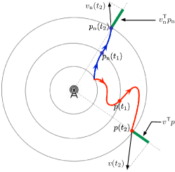
Figure 1: Nominal (blue) and undetectable attack (red) trajectories. At all times, the two trajectories have equal distance from the base station, and equal velocity components along the direction of the instantaneous position (green segments).

Theorem 7.

(Implicit characterization of undetectable attacks) The attack $(u,{u}^{\textup{GNSS}})$ is undetectable if and only if

$$u^{\mathsf{T}}p={u}_{\textup{n}}^{\mathsf{T}}{p}_{\textup{n}}+\|{v}_{\textup{n}}\|^{2}-\|v\|^{2},\text{ and }{u}^{\textup{GNSS}}={p}_{\textup{n}}-p.$$ (6)

(Only if) By substitution of (2) and (4) into Definition 2 we readily obtain $p+{u}^{\textup{GNSS}}={p}_{\textup{n}}$, from which the second identity in the statement follows. To show the first identity, we note that for every undetectable attack $u$ the identity ${y}^{\textup{RSSI}}-{y}^{\textup{RSSI}}_{\text{n}}=0$ holds. We then make explicit the dependence on the control input in the above identity by taking the second-order derivative with respect to time. This yields ${\ddot{y}}^{\textup{RSSI}}-{\ddot{y}}^{\textup{RSSI}}_{\text{n}}=0$. Then,

$$0={\ddot{y}}^{\textup{RSSI}}-{\ddot{y}}^{\textup{RSSI}}_{\text{n}}=2u^{\mathsf{T}}p+2v^{\mathsf{T}}v-2{u}_{\textup{n}}^{\mathsf{T}}{u}_{\textup{n}}-2{v}_{\textup{n}}^{\mathsf{T}}{v}_{\textup{n}},$$

from which (6) follows. We emphasize that the functions ${\dot{y}}^{\textup{RSSI}}$, ${\ddot{y}}^{\textup{RSSI}}$, ${\dot{y}}^{\textup{RSSI}}_{\text{n}}$, ${\ddot{y}}^{\textup{RSSI}}_{\text{n}}$ are piecewise continuous functions, since the signals ${y}^{\textup{RSSI}}$ and ${y}^{\textup{RSSI}}_{\text{n}}$ are continuous and twice differentiable at all times. To see this, we combine the piecewise continuity assumption on ${u}_{\textup{n}}$ and $u$ with the dynamical equations (1) and (3), and note that the velocities ${v}_{\textup{n}}$ and $v$ and the positions ${p}_{\textup{n}}$ and $p$ are continuous and differentiable functions of time.

(If) Let ${u}^{\textup{GNSS}}={p}_{\textup{n}}-p$. Substituting into (4) yields

$${y}^{\textup{GNSS}}-{y}^{\textup{GNSS}}_{\text{n}}=p+{u}^{\textup{GNSS}}-{p}_{\textup{n}}=0,$$

from which the first condition in Definition 2 follows. To prove RSSI undetectability, let $u$ satisfy (6). Then,

$${\ddot{y}}^{\textup{RSSI}}-{\ddot{y}}^{\textup{RSSI}}_{\text{n}}=2u^{\mathsf{T}}p+2v^{\mathsf{T}}v-2{u}_{\textup{n}}^{\mathsf{T}}{p}_{\textup{n}}-2{v}_{\textup{n}}^{\mathsf{T}}{v}_{\textup{n}}=0,$$

from which we readily obtain the identity ${\ddot{y}}^{\textup{RSSI}}-{\ddot{y}}^{\textup{RSSI}}_{\text{n}}=0$. Since the functions ${y}^{\textup{RSSI}}$ and ${y}^{\textup{RSSI}}_{\text{n}}$ are continuous and twice differentiable, and the initial conditions satisfy $p(0)=p_{\text{n}}(0)$ and $v(0)=v_{\text{n}}(0)$ we conclude that ${\dot{y}}^{\textup{RSSI}}-{\dot{y}}^{\textup{RSSI}}_{\text{n}}=0$ and ${y}^{\textup{RSSI}}-{y}^{\textup{RSSI}}_{\text{n}}=0$. Thus, ${y}^{\textup{RSSI}}={y}^{\textup{RSSI}}_{\text{n}}$ at all times, which implies undetectability of the attack $u$ and concludes the proof. $\blacksquare$

Finally, we exploit Theorem 7 to give an explicit and comprehensive characterization of undetectable attacks.

Corollary 8.

(Explicit characterization of undetectable attacks) The attack $(u,{u}^{\textup{GNSS}})$ is undetectable if and only if it satisfies

$$u={a}_{\textup{r }}p+w\text{ and }{u}^{\textup{GNSS}}={p}_{\textup{n}}-p,$$ (7)

whenever $\|p\|\neq 0$, where $w^{\mathsf{T}}p=0$ and

$${a}_{\textup{r}}=\frac{{u}_{\textup{n}}^{\mathsf{T}}{p}_{\textup{n}}+\|{v}_{\textup{n}}\|^{2}-\|v\|^{2}}{\|p\|^{2}}.$$

Corollary 8 provides a systematic way to design undetectable attacks by designing the attack inputs $(u,{u}^{\textup{GNSS}})$. We also note that the input $w$ can be arbitrarily selected by the attacker and it does not affect detectability of the attack. Finally, it should be noticed that ${a}_{\textup{r}}$ corresponds to the radial acceleration of the robot, that is, the projection of $u$ along $p$, and that the attack input $u$ is unconstrained when $\|p\|=0$ (see also Theorem 7).

4 Design of optimal undetectable attacks

In this section we design undetectable attacks that introduce maximal deviations between the nominal and attacked trajectories. Assuming that the attacker knows the nominal control input, we address the optimal control problem

$$\underset{w}{\text{max}} \|p(T)-p_{\text{n}}(T)\|,$$

subject to $$\dot{x}=Ax+Bu,$$ (8a)

$$u={a}_{\textup{r }}p+w,$$ (8b)

$${a}_{\textup{r}}=({u}_{\textup{n}}^{\mathsf{T}}{p}_{\textup{n}}+\|{v}_{\textup{n}}\|^{2}-\|v\|^{2})\|p\|^{-2},$$ (8c)

$$\|u\|\leq{u}_{\textup{max}}.$$ (8d)

In the maximization problem (8), constraint (8a) corresponds to the attacked dynamics (3), while (8b)-(8c) enforce attack-undetectability from Corollary 8. We next characterize the optimality conditions of the problem (8). Let $e_{i}$ denote the $i$-th canonical vector of appropriate dimension, and let $\operatorname{sgn(~{})}$ denote the sign function.

Theorem 9.

(Attack optimality conditions) Let ${a}_{\textup{r}}$ be as in (8c), and let $w^{*}$ be an optimal solution to (8). Then,

$$w^{*}={a}_{\textup{t}}Wx,$$

where

$${a}_{\textup{t}} =-\operatorname{sgn}(\lambda^{\mathsf{T}}B\mathrm{W}x)\sqrt{{u}_{\textup{max}}^{2}/\|p\|^{2}-{a}_{\textup{r}}^{2}},$$

$$W =\begin{bmatrix}-e_{2}&e_{1}&0_{2}&0_{2}\end{bmatrix},$$

and $\lambda$ and $x$ satisfy

$$\dot{x} =Ax+{a}_{\textup{r}}Bp+Bw^{*},$$

$$-\dot{\lambda} =(A^{\mathsf{T}}\lambda+{a}_{\textup{r}}\tilde{P}+{a}_{\textup{t}}\tilde{W})\lambda+(x^{\mathsf{T}}\tilde{P}\lambda+2{a}_{\textup{r}}\nu\|{p}_{\textup{n}}\|^{2})\nabla_{x}{a}_{\textup{r}},$$

with boundary conditions

$$x(0)={x}_{\textup{n}}(0),\text{ and }\lambda(T)=-2[(p(T)-{p}_{\textup{n}}(T))^{\mathsf{T}}~{}0_{2}^{\mathsf{T}}]^{\mathsf{T}},$$

where $\tilde{P}=P^{\mathsf{T}}B^{\mathsf{T}}$, $\tilde{W}=W^{\mathsf{T}}B^{\mathsf{T}}$, $\nabla_{x}{a}_{\textup{r}}=2\|p\|^{-2}[0_{2}^{\mathsf{T}}~{}v^{\mathsf{T}}]^{\mathsf{T}},$ and $\nu=-\frac{\lambda^{\mathsf{T}}B\mathrm{W}x}{2{a}_{\textup{t}}\|p\|^{2}}$.

To formalize the result, we make use of the fact that any undetectable attack (7) can be written in the form

$$u={a}_{\textup{r }}\mathrm{P}x+{a}_{\textup{t }}\mathrm{W}x,$$ (9)

where $\mathrm{P}=[e_{1}~{}e_{2}~{}0~{}0]\in{}^{2\times 4}$, $\mathrm{W}=[-e_{2}~{}e_{1}~{}0~{}0]\in{}^{2\times 4}$, and ${a}_{\textup{t}}:\mathbb{R}_{\geq 0}\rightarrow\real$. Following expression (9), the function ${a}_{\textup{t}}$ represents the new design parameter in the optimization problem. To derive the optimality conditions for (8), we use the Pontryagin’s Maximum Principle [25], combined with the direct adjoining method for mixed state-input constraints [26]. We incorporate (8b) and (9) into (8a) and define the Hamiltonian

$$\mathcal{H}(x,{a}_{\textup{t}},\lambda,t)=\lambda^{\mathsf{T}}(Ax+B({a}_{\textup{r}}\mathrm{P}x+{a}_{\textup{t}}\mathrm{W}x)),$$

where $\lambda:[0,T]\rightarrow{}^{4}$ is a vector function of system costates, with the additional constraints

$$x(0)={x}_{\textup{n}}(0),{a}_{\textup{r}}=\frac{{u}_{\textup{n}}^{\mathsf{T}}{p}_{\textup{n}}+\|{v}_{\textup{n}}\|^{2}-\|v\|^{2}}{\|p\|^{2}},\|u\|\leq{u}_{\textup{max}}.$$

We then use (9) to rewrite the bound $\|u\|\leq{u}_{\textup{max}}$ as

$${a}_{\textup{r}}^{2}\|{p}_{\textup{n}}\|^{2}+{a}_{\textup{t}}^{2}\|{p}_{\textup{n}}\|^{2}\leq{u}_{\textup{max}}^{2},$$

and form the Lagrangian by adjoining the Hamiltonian with the considered state constraint:

$$\mathcal{L}(x,{a}_{\textup{t}},\lambda,t,\nu)=\mathcal{H}(x,{a}_{\textup{t}}, \lambda,t)+$$

$$\nu({a}_{\textup{r}}^{2}\|{p}_{\textup{n}}\|^{2}+{a}_{\textup{t}}^{2}\|{p}_{\textup{n}}\|^{2}-{u}_{\textup{max}}^{2}),$$

where $\nu:[0,T]\rightarrow\real$ is the Lagrange multiplier associated with the state constraint.

By application of the Maximum Principle [26], the optimal control input ${a}_{\textup{t}}^{*}$ minimizes the Hamiltonian over the set $U(x)=\{{a}_{\textup{t}}:{a}_{\textup{r}}^{2}\|p\|^{2}+{a}_{\textup{t}}^{2}\|p\|^{2}\leq{u}_{\textup{max}}^{2}\}$, that is, ${a}_{\textup{t}}^{*}=\operatorname{arg}\min_{{a}_{\textup{t}}\in U(x)}\mathcal{H}(x,{a}_{\textup{t}},\lambda,t)$. This fact yields the optimal control law

$${a}_{\textup{t}}^{*}=-\operatorname{sgn}(\lambda^{\mathsf{T}}B\mathrm{W}x)\sqrt{{u}_{\textup{max}}^{2}/\|p\|^{2}-{a}_{\textup{r}}^{2}}.$$

Moreover, it follows from the Maximum Principle that there exists a vector function of system costates $\lambda$ that satisfies the following system of equations

$$\dot{x} =\frac{\partial\mathcal{L}}{\partial\lambda}\Rightarrow\;\;\;\dot{x}=Ax+B({a}_{\textup{r }}\mathrm{P}x+{a}_{\textup{t}}\mathrm{W}x),$$

$$-\dot{\lambda} =\frac{\partial\mathcal{L}}{\partial x}\Rightarrow\begin{aligned} -\dot{\lambda}=&A^{\mathsf{T}}\lambda+{a}_{\textup{r}}P^{\mathsf{T}}B^{\mathsf{T}}\lambda+x^{\mathsf{T}}P^{\mathsf{T}}B^{\mathsf{T}}\lambda\nabla_{x}{a}_{\textup{r}}+\\ &{a}_{\textup{t}}W^{\mathsf{T}}B^{\mathsf{T}}\lambda+2{a}_{\textup{r}}\nu\|{p}_{\textup{n}}\|^{2}\nabla_{x}{a}_{\textup{r}}\end{aligned}$$

$$0 =\frac{\partial\mathcal{L}}{\partial{a}_{\textup{t}}}\Rightarrow\;\;\;0=\lambda^{\mathsf{T}}B\mathrm{W}x+2\nu{a}_{\textup{t}}\|p\|^{2},$$

where $\nabla_{x}{a}_{\textup{r}}$ denotes the gradient of ${a}_{\textup{r}}$ with respect to $x$, and with boundary conditions

$$x(0)\;={x}_{\textup{n}}(0),\text{ and }\lambda(T)=\frac{\partial}{\partial x}\|p(T)-p_{\text{n}}(T)\|.$$

The statement of the theorem follows by substituting the expression of the gradient $\nabla_{x}{a}_{\textup{r}}=2\|p\|^{-2}[0~{}0~{}v^{\mathsf{T}}]^{\mathsf{T}}$. $\blacksquare$

From Theorem 9, optimal undetectable attacks can be computed by solving a two-point boundary value problem [27]. This class of problems is typically solved numerically, and it may lead to numerical difficulties for general cases [27]. To conclude this section and provide some intuition in the design of optimal undetectable attacks, we next present an example where optimal attacks can be characterized explicitly.

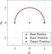
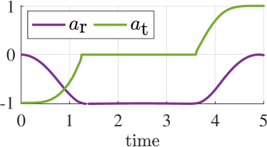
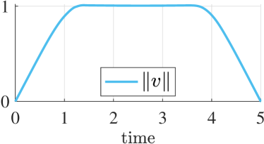
Figure 2: For an idle robot at position $(1,0)$ (blue dot), (a) shows an optimal undetectable attack trajectory, which maintains a distance equal to $1$ from the base station and maximises the distance from the nominal position. Fig. (b) shows the radial and tangential components of the acceleration. Fig. (c) shows the velocity of the attacked robot, which becomes zero when the robot reaches the final point $(-1,0)$.

Example 10.

(Undetectable trajectories for idle robots) Let ${p}_{\textup{n}}(0)=[1~{}0]^{\mathsf{T}}$, ${v}_{\textup{n}}(0)=0$, and ${u}_{\textup{n}}=0$, so that the robot remains at position ${p}_{\textup{n}}(0)$ at all times. Let ${u}_{\textup{max}}=1$ and $T=5$. Under these assumptions, the following control inputs satisfy the optimality conditions in Theorem 9:

$${a}_{\textup{t}}^{*}=\begin{cases}\zeta\sqrt{{u}_{\textup{max}}^{2}-{a}_{\textup{r}}^{2}},&t\in[0,\tau],\\ -\zeta\sqrt{{u}_{\textup{max}}^{2}-{a}_{\textup{r}}^{2}},&t\in[\tau,T],\end{cases}\text{ and }{a}_{\textup{r}}=-\|v\|^{2},$$ (10)

where $\tau=3.475$, and $\zeta\in\{-1,1\}$. It is worth noting that, because at every time the radial acceleration is proportional to the square of the magnitude of the velocity, the control input (10) leads the attacked robot to perform a circular motion around the origin (see Fig. 2). Notice that $\zeta=-1$ and $\zeta=1$ achieve counterclockwise and clockwise motion, respectively. Finally, (10) is an optimal solution to the optimization problem (8) since the deviation $\|p(T)-p_{\text{n}}(T)\|$ is maximized, as graphically illustrated in Fig. 2.

To derive the value of the final time $\tau$,we can explicitly derive a an expression for the magnitude of the velocity vector $n:=\|v\|$, that reads $\dot{n}=\sqrt{{u}_{\textup{max}}^{2}-n^{2}}$, where we have substituted the expression for ${a}_{\textup{r}}$ into ${a}_{\textup{t}}^{*}$, and used the fact that $n$ is independent of ${a}_{\textup{r}}$. To obtain the value of $\tau$, we seek for the time needed to steer $n(t)$ from ${u}_{\textup{max}}$ to a full stop, by letting $n(0)={u}_{\textup{max}}$ and $n(\tau)=0$. $\square$

We show in Fig. 3 a set of simulations that illustrate the effects of optimal attacks (red) when the nominal trajectory is the shortest path between the initial and the final position (blue). In particular, the figure demonstrates that increasing levels of deviation are achieved by the attacker when the trajectory planner employs control inputs with decreasing magnitude (i.e., different and decreasing fractions of ${u}_{\textup{max}}$).

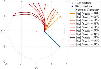
Figure 3: For a nominal straight line trajectory (blue), the figure shows the undetectable attack trajectories obtained from Theorem 9 for different values of the nominal acceleration $\|{u}_{\textup{n}}\|/{u}_{\textup{max}}$. As the nominal acceleration decreases, the deviation induced by an optimal attack increases. Simulation parameters: $T=1.5$, $v(0)=0$, and ${u}_{\textup{n}}=[1,-1]^{\mathsf{T}}$ at all times.

5 Design of secure trajectories

In this section we address the secure trajectory planning problem. First, we characterize the existence of secure trajectories as a function of the initial and final configurations of the robot. Then, we formulate and solve an optimization problem to design control inputs that generate secure trajectories to reach a desired final configuration. We start with some necessary definitions. We say that a trajectory ${x}_{\textup{n}}$ is secure if, independently of the attack $u$, one of the following mutually exclusive conditions is satisfied:

1. $p=p_{\text{n}}$ at all times; or

2. if $p\neq p_{\text{n}}$ at some time, the attack $u$ is detectable.

Similarly, a control input is secure if it generates a secure trajectory. We next characterize secure control inputs explicitly.

Theorem 11.

(Secure control inputs) Let ${x}_{\textup{n}}$ be the trajectory generated by ${u}_{\textup{n}}$. Then, ${u}_{\textup{n}}$ is secure if and only if the following conditions hold simultaneously:

1. there exists a function $\kappa:\mathbb{R}_{\geq 0}\rightarrow\{-1,1\}$ satisfying

   $$u_{\text{n}}=\kappa\frac{p_{\text{n}}}{\|p_{\text{n}}\|}{u}_{\textup{max}},$$ (11)

2. the trajectory ${x}_{\textup{n}}$ satisfies $p_{\text{n}}\neq 0$ at all times.

(If) We assume (1)-(2) and show that either (C1) or (C2) is satisfied. We distinguish among two cases.
(Case 1) The attack $(u,{u}^{\textup{GNSS}})$ does not satisfy the undetectability condition (6). Then, (C2) follows.
(Case 2) The attack $(u,{u}^{\textup{GNSS}})$ satisfies the undetectability condition (6). Under this assumption we now show that (1)-(2) imply (C1). We first consider the time instant $\tau=0$. By using the assumption ${x}_{\textup{n}}(\tau)=x(\tau)$, which yields ${p}_{\textup{n}}(\tau)=p(\tau)$ and $\|{v}_{\textup{n}}(\tau)\|=\|v(\tau)\|$, and by substituting into (6) we obtain the following undetectability condition valid at time $\tau$:

$${u}_{\textup{n}}^{\mathsf{T}}(\tau){p}_{\textup{n}}(\tau)=u^{\mathsf{T}}(\tau)p(\tau).$$ (12)

By taking the $2$-norm on both sides of the above equality, and by substituting the expression (11) we obtain

$${u}_{\textup{max}}\|{p}_{\textup{n}}(\tau)\|=|{u}_{\textup{n}}(\tau)^{\mathsf{T}} {p}_{\textup{n}}(\tau)|=$$

$$|u^{\mathsf{T}}(\tau)p(\tau)|\leq{u}_{\textup{max}}\|p(\tau)\|,$$

where we used the Cauchy-Schwarz inequality. Since exact equality must hold, the vectors $u(\tau)$ and $p(\tau)$ are linearly dependent and $\|u(\tau)\|={u}_{\textup{max}}$, that is,

$$u(\tau)=\gamma(\tau)\frac{p(\tau)}{\|p(\tau)\|}{u}_{\textup{max}},$$

where $\gamma(\tau)\in\{-1,1\}$. Finally, we note that $\gamma(\tau)\neq\kappa(\tau)$ results in a violation of (12), and therefore $u(\tau)={u}_{\textup{n}}(\tau)$. As a result, ${p}_{\textup{n}}(\tau^{+})=p(\tau^{+})$. To conclude the proof, we iterate the above reasoning for all $\tau\in[0,T)$, from which (C1) follows.

(Only if) We show that (C1)-(C2) imply (1)-(2) or, equivalently, if (1)-(2) do not simultaneously hold, then (C1)-(C2) are not satisfied. We distinguish two cases.
(Case 1) Let ${\bar{u}}_{\textup{n}}$ be any control input that does not satisfy (11). That is, there exists $\bar{t}\in[0,T]$, such that

$${\bar{u}}_{\textup{n}}(t)={u}_{\textup{n}}(t)\text{ for all }t\in[0,\bar{t}),\quad\text{ and }\quad{\bar{u}}_{\textup{n}}(\bar{t})\neq u_{\text{n}}(\bar{t}).$$

Let $\bar{u}$ be an attack input, with $\bar{u}={\bar{a}}_{\textup{r }}p+\bar{w}$ as in Corollary 8. We take the absolute value of (7) and use the relationship $\|{v}_{\textup{n}}(\bar{t})\|=\|v(\bar{t})\|$ to obtain the inequality

$$|{\bar{a}}_{\textup{r}}(\bar{t})|=\frac{|{\bar{u}}_{\textup{n}}^{\mathsf{T}}(\bar{t}){p}_{\textup{n}}(\bar{t})|}{\|p(\bar{t})\|}<{u}_{\textup{max}},$$

where strict inequality follows from the assumption ${\bar{u}}_{\textup{n}}(\bar{t})\neq u_{\text{n}}(\bar{t})$. As a result, any vector $\bar{w}$ that satisfies $\|{\bar{a}}_{\textup{r}}(\tau)p(\tau)+\bar{w}(\tau)\|={u}_{\textup{max}}$, is a nonzero undetectable attack that violates (C1) and (C2).
(Case 2) There exists $\bar{t}\in[0,T]$, such that $\|{p}_{\textup{n}}(\bar{t})\|=0$. It follows from (6) that whenever ${p}_{\textup{n}}(\bar{t})=0$ any attack input is unconstrained at time instant $\bar{t}$. As a result, any $u$ with $u(t)={u}_{\textup{n}}(t)$ for all $t\in[0,\bar{t})$ and $u(\bar{t})\neq{u}_{\textup{n}}(\bar{t})$ is undetectable and violates (C1) and (C2). $\blacksquare$

Theorem 11 provides an explicit characterization of secure control inputs, and it shows that any secure control input has maximum magnitude ${u}_{\textup{max}}$ at all times, and its direction is aligned with the direction of the positioning vector. We next show that any secure trajectory evolves on an invariant manifold of the state space that is uniquely defined by the initial state of the robot.

Lemma 12.

(Invariant manifold of secure trajectories) Let ${x}_{\textup{n}}$ be the trajectory generated by the secure control input ${u}_{\textup{n}}$. Then, ${x}_{\textup{n}}\in\mathcal{S}$ at all times, where

$$\mathcal{S}=\{x\;:\;x_{1}x_{4}-x_{2}x_{3}=x_{1}(0)x_{4}(0)-x_{2}(0)x_{3}(0)\}.$$

Let ${x}_{\textup{n}}=[x_{1}~{}x_{2}~{}x_{3}~{}x_{4}]^{\mathsf{T}}$ denote the solution to (1) with initial condition ${x}_{\textup{n}}(0)$, subject to control inputs that satisfy (1)-(2) in Theorem 11. To prove that ${x}_{\textup{n}}\in\mathcal{S}$, we equivalently show that the quantity $x_{1}x_{4}-x_{2}x_{3}$ is time-invariant, that is, $\frac{d}{dt}(x_{1}x_{4}-x_{2}x_{3})=0$. In fact,

$$\dot{x}_{1}x_{4}+x_{1}\dot{x}_{4}-\dot{x}_{2}x_{3}-x_{2}\dot{x}_{3}=0,$$

where the last equality follows by substitution of (1). $\blacksquare$

Lemma 12 shows that secure trajectories are constrained to evolve on a manifold that is defined by the initial state of the robot, and it implies that only a subset of the state space can be reached via secure trajectories. These observations are illustrated in the next example.

Example 13.

(Reachable configurations) Let ${x}_{\textup{n}}(0)=[\bar{x}_{1}~{}0~{}\bar{x}_{3}~{}0]^{\mathsf{T}}$, where $\bar{x}_{1}\in{}_{>0}$ and $\bar{x}_{3}\in\real$, that is, let the robot at time $t=0$ be located on the horizontal axis, with initial velocity in the horizontal direction. From Lemma 12, every secure trajectory satisfied ${x}_{\textup{n}}\in\mathcal{S}$ at all times, with

$$\mathcal{S}=\{x\;:\;x_{1}x_{4}-x_{2}x_{3}=0\}.$$

It should be observed, however, that secure trajectories may in fact be constrained on a strict subset of $\mathcal{S}$. In fact, by combining the system dynamics (1) with the secure control input (11), we obtain

$$x_{1}>0,\quad x_{2}=0,\quad x_{4}=0,$$

which is a strict subset of $\mathcal{S}$. Notice that the above equations imply that the motion of the robot under secure control inputs is constrained on the positive $x$-axis. $\square$

To determine a secure trajectory from the initial position ${p}_{\textup{I}}$ with given velocity ${v}_{\textup{I}}$ towards the final position ${p}_{\textup{F}}$, we consider the optimization problem

$$\underset{\kappa,T}{\text{min}} T~{}+~{}\|{p}_{\textup{n}}(T)-{p}_{\textup{F}}\|,$$

subject to $${\dot{x}}_{\textup{n}}=A{x}_{\textup{n}}+B{u}_{\textup{n}},$$

$${p}_{\textup{n}}(0)={p}_{\textup{I}},{v}_{\textup{n}}(0)={v}_{\textup{I}},$$

$$u_{\text{n}}=\kappa\frac{p_{\text{n}}}{\|p_{\text{n}}\|}u_{\text{max}},$$ (13)

which aims to find a secure control input that minimizes a weighted combination of the distance to the desired final position and the time needed to reach such position. The following result characterizes the solutions to the optimization problem (13).

Theorem 14.

(Optimality conditions for secure control inputs) Let $\kappa^{*}$ and $T^{*}$ be an optimal solution to (13). Then,

$$\kappa^{*}=-\operatorname{sgn}(\lambda^{\mathsf{T}}B{p}_{\textup{n}}),\text{ and }T^{*}=\xi,$$

where $\xi\in{}_{>0}$, ${x}_{\textup{n}}$, and $\lambda$ satisfy

$${\dot{x}}_{\textup{n}} =\xi(A{x}_{\textup{n}}+\frac{\kappa^{*}~{}{u}_{\textup{max}}}{\|{p}_{\textup{n}}\|}B{p}_{\textup{n}}),$$

$$-\dot{\lambda} =\xi(A^{\mathsf{T}}\lambda+\frac{\kappa^{*}~{}{u}_{\textup{max}}}{\|{p}_{\textup{n}}\|^{3}}\Phi({p}_{\textup{n}})B^{\mathsf{T}}\lambda),$$

$$\dot{\xi} =0,$$ (14)

for all $t\in[0,1]$, with boundary conditions

$${x}_{\textup{n}}(0)=x_{0},$$

$$\lambda(1)=2[(p(T)-{p}_{\textup{n}}(T))^{\mathsf{T}}0_{2}^{\mathsf{T}}]^{\mathsf{T}},$$

$$\lambda(0)(Ax_{0}+B\kappa^{*}(0)\frac{p_{\text{n}}(0)}{\|p_{\text{n}}(0)\|}u_{\text{max}})=-1,$$

and

$$\Phi({p}_{\textup{n}})=\left(\|{p}_{\textup{n}}\|^{2}I_{2}-2{p}_{\textup{n}}{p}_{\textup{n}}^{\mathsf{T}}\right)\begin{bmatrix}I_{2}&\boldsymbol{0}_{2}\\ \boldsymbol{0}_{2}&\boldsymbol{0}_{2}\end{bmatrix}.$$

To determine the unknown final time $T$ we employ a technique similar to [28] and let $t=\xi\tau$, where $\xi\in{}_{>0}$ is a constant unknown parameter, and $\tau$ is the new temporal variable, with $0\leq\tau\leq 1$. We then use The Pontryagin’s Maximum Principle [25] to derive the optimality conditions for the optimization problem (13), and consider the Hamiltonian

$$\mathcal{H}({x}_{\textup{n}},\kappa,\lambda)=1+\lambda^{\mathsf{T}}\xi(A{x}_{\textup{n}}+B{u}_{\textup{n}}),$$

where $\lambda$ is the vector function of system costates. By application of the Maximum Principle [25], the optimal control input and corresponding trajectory satisfy the following optimality conditions

$${\dot{x}}_{\textup{n}} =\frac{\partial\mathcal{H}}{\partial\lambda}\Rightarrow\;\;{\dot{x}}_{\textup{n}}=\xi(A{x}_{\textup{n}}+B{u}_{\textup{n}}),$$

$$-\dot{\lambda} =\frac{\partial\mathcal{H}}{\partial{x}_{\textup{n}}}\Rightarrow-\dot{\lambda}=\xi(A^{\mathsf{T}}\lambda+\frac{\partial{u}_{\textup{n}}}{\partial{x}_{\textup{n}}}B^{\mathsf{T}}\lambda),$$

with boundary conditions ${x}_{\textup{n}}(0)\;=x_{0}$ and $\lambda(1)=\frac{\partial V}{\partial x}(x(1))$, where we used the fact $0\leq\tau\leq 1$. To derive an expression for the partial derivative of ${u}_{\textup{n}}$ with respect to ${x}_{\textup{n}}$ we let $\mathrm{P}=[e_{1}~{}e_{2}~{}0~{}0]\in{}^{2\times 4}$ and rewrite (11) as

$$u_{\text{n}}=\kappa\frac{\mathrm{P}x_{\text{n}}}{\|\mathrm{P}x_{\text{n}}\|}u_{\text{max}},$$

which yields

$$\frac{\partial{u}_{\textup{n}}}{\partial{x}_{\textup{n}}}=\frac{\kappa{u}_{\textup{max}}}{\|{p}_{\textup{n}}\|}\mathrm{P}-2\frac{\kappa{u}_{\textup{max}}}{\|{p}_{\textup{n}}\|^{3}}\mathrm{P}{x}_{\textup{n}}{x}_{\textup{n}}^{\mathsf{T}}\mathrm{P}^{\mathsf{T}}\mathrm{P}.$$

Hence, the expression for $\Phi({p}_{\textup{n}})$ follows by substitution.

To determine the unknown final time, we consider the additional differential equation $\dot{\xi}=0$, and let $\xi$ be an unknown parameter. In particular, to determine the additional boundary condition we use the fact that the Hamiltonian is independent of time and the final time is free. Thus, the Hamiltonian is a first integral along optimal trajectories [25], i.e., $\mathcal{H}({x}_{\textup{n}},\kappa,\lambda)=\text{const.}$, with $\mathcal{H}({x}_{\textup{n}},\kappa,\lambda)|_{t=0}=0$, which yield the claimed boundary conditions and the statement follows. $\blacksquare$

Theorem 14 allows us to compute secure control inputs by solving a two-point boundary value problem [27]. We propose in Fig. 4 (see also corresponding data in Table 1) a comparison between a secure trajectory and a minimum time trajectory (non secure). In particular, a minimum-time trajectory is obtained by numerically solving the following optimization problem

$$\underset{{u}_{\textup{n}},T}{\text{min}} T~{}+~{}\|{p}_{\textup{n}}(T)-{p}_{\textup{F}}\|,$$

subject to $${\dot{x}}_{\textup{n}}=A{x}_{\textup{n}}+B{u}_{\textup{n}},$$

$${p}_{\textup{n}}(0)={p}_{\textup{I}},{v}_{\textup{n}}(0)={v}_{\textup{I}},$$

We note that secure trajectory require longer control horizons but, differently from minimum-time trajectories, prevent the existence of undetectable attacks.

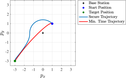
Figure 4: (a) Secure (blue) and minimum time (red) trajectories between ${p}_{\textup{I}}=(1,1)$ and ${p}_{\textup{F}}=(-3,-3)$, with $v(0)=[-1,1]^{\mathsf{T}}$ and ${u}_{\textup{max}}=1$. (b) and (c) Corresponding control inputs. Note that for minimum time trajectories, vectors ${u}_{\textup{n}}$ and ${p}_{\textup{n}}$ are not aligned at all times.

	(Time)	(Attack Deviation)
	$T$	$\underset{w}{\text{max}}\|p(T)-p_{\text{n}}(T)\|$
Min. time trajectory	$1.5$	$8.49$
Secure trajectory	$3.84$	$0$

Table 1: Details for minimum-time and secure trajectories in Fig. 4.

6 Undetectable attacks and secure trajectories for robots with unicycle dynamics

The goal of this section is to characterize undetectable attacks and secure trajectories for robots with unicycle dynamics, so as to illustrate that the methods developed in this paper are applicable to a broad and general class of robot models. A robot with unicycle dynamics has one steerable drive wheel [29], and is modeled through the dynamical equations

$$\dot{p}_{\text{n}}^{x} ={\nu}_{\textup{n}}\cos({\theta}_{\textup{n}}),\;\dot{p}_{\text{n}}^{y}={\nu}_{\textup{n}}\sin({\theta}_{\textup{n}}),\;{\dot{\theta}}_{\textup{n}}={\omega}_{\textup{n}},$$

where ${p}_{\textup{n}}=[p_{\text{n}}^{x}~{}p_{\text{n}}^{y}]:\mathbb{R}_{\geq 0}\rightarrow{}^{2}$ denotes the robot position, $\theta_{\text{n}}:\mathbb{R}_{\geq 0}\rightarrow[0,2\pi)$ denotes the steering angle, ${\nu}_{\textup{n}}:\mathbb{R}_{\geq 0}\rightarrow\mathbb{R}_{\geq 0}$ and ${\omega}_{\textup{n}}:\mathbb{R}_{\geq 0}\rightarrow\real$ denote the wheel velocity and steering control, respectively. We assume that ${\nu}_{\textup{n}}$ is differentiable, ${\omega}_{\textup{n}}$ is piecewise continuous, and that ${\nu}_{\textup{n}}\leq{\nu}_{\textup{max}}$ and $|{\omega}_{\textup{n}}|\leq{\omega}_{\textup{max}}$, where ${\nu}_{\textup{max}}\in{}_{>0}$ and ${\omega}_{\textup{max}}\in{}_{>0}$. Similarly to (3), we model the unicycle dynamics in the presence of attacks as

$$\dot{p}^{x} =\nu\cos(\theta),\;\dot{p}^{y}=\nu\sin(\theta),\;\dot{\theta}=\omega,$$

where $p=[p^{x}~{}p^{y}]:\mathbb{R}_{\geq 0}\rightarrow{}^{2}$ and $\theta:\mathbb{R}_{\geq 0}\rightarrow[0,2\pi)$ denote, respectively, the position and steering angle of the robot under attack, while $\nu:\mathbb{R}_{\geq 0}\rightarrow\mathbb{R}_{\geq 0}$ and $\omega:\mathbb{R}_{\geq 0}\rightarrow\real$ denote the attacked wheel velocity and steering control. As described in Section 2, we assume that the robot is equipped with a GNSS and an RSSI sensor, whose measurements are as in (2) in the absence of attacks, and as in (4) in the presence of attacks.

Using the notions in Definition 2, we next characterize undetectable attacks against robots with unicycle dynamics. In the remainder of this section, we let $\operatorname{angle}(v,w)$ denote the angle between the vectors $v$ and $w$, that is

$$\operatorname{angle}(v,w)=\arccos\left(\frac{v^{\mathsf{T}}w}{\|v\|\|w\|}\right),$$

with $\operatorname{angle}(0,w)=\operatorname{angle}(v,0)=0$.

Theorem 15.

(Undetectable attacks for unicycle dynamics) Let ${\phi}_{\textup{n}}=\operatorname{angle}({p}_{\textup{n}},{\dot{p}}_{\textup{n}})$ and $\phi=\operatorname{angle}(p,\dot{p})$. The attack $(\nu,\omega,{u}^{\textup{GNSS}})$ is undetectable if and only if

$$\nu\cos(\phi)={\nu}_{\textup{n}}\cos({\phi}_{\textup{n}}),\text{ and }{u}^{\textup{GNSS}}={p}_{\textup{n}}-p.$$ (15)

The proof follows by extending the proof of Theorem 7 to the considered unycicle dynamics. $\blacksquare$

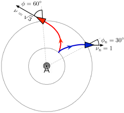
Figure 5: Nominal (blue) and undetectable attack (red) trajectories. As discussed in Theorem 15, the illustrated vectors satisfy $\nu\cos(\phi)={\nu}_{\textup{n}}\cos({\phi}_{\textup{n}})$ to guarantee undetectability.

An example where the condition in Theorem 15 holds is illustrated in Fig. 5. Next, we provide a characterization of secure control inputs for unicycle dynamics.

Theorem 16.

(Secure control inputs for unicycle dynamics) Let ${\phi}_{\textup{n}}=\operatorname{angle}({p}_{\textup{n}},{\dot{p}}_{\textup{n}})$. The control input $({\nu}_{\textup{n}},{\omega}_{\textup{n}})$ is secure if and only if the following conditions hold simultaneously:

1. ${\phi}_{\textup{n}}(0)\in\{0,\pi\}$, and $p_{\text{n}}\neq 0$ at all times,

2. $\nu_{\text{n}}=\nu_{\text{max}}$ and $\omega_{\text{n}}=0$ at all times.

(If) We assume (1)-(2) and show that either (C1) or (C2) is satisfied. We distinguish among two cases.
(Case 1) The attack $(\nu,\omega,{u}^{\textup{GNSS}})$ does not satisfy (15). Then, (C2) immediately follows.
(Case 2) The attack $(\nu,\omega,{u}^{\textup{GNSS}})$ satisfies (15). We first focus on the time instant $\tau=0$, and take the absolute value on both sides of the undetectability condition (15) to obtain the identity

$$|{\nu}_{\textup{n}}(0)\cos({\phi}_{\textup{n}}(0))|=|\nu(0)\cos(\phi(0))|.$$ (16)

By substituting conditions (1)-(2) into the left-hand side of (16) we obtain

$$|{\nu}_{\textup{n}}(0)\cos({\phi}_{\textup{n}}(0))|={\nu}_{\textup{max}}.$$

On the other hand, by applying the Cauchy-Schwartz inequality to the right-hand side of (16) we have

$$|\nu(0)\cos(\phi(0))|\leq|\nu(0)||\cos(\phi(0))|\leq{\nu}_{\textup{max}}.$$

By application of (16), exact equality must hold in the above bound, and thus we necessarily have $\nu(0)={\nu}_{\textup{max}}$ and $|\cos(\phi(0))|=1$. Finally, we use the fact that $\phi$ is a differentiable function of time to obtain $\phi(0)={\phi}_{\textup{n}}(0)$. To conclude the proof, we use the fact that ${\omega}_{\textup{n}}=0$ at all times, which implies ${\phi}_{\textup{n}}(\tau)={\phi}_{\textup{n}}(0)$ for all $\tau$ (a formal proof of this fact can be done by leveraging the change of variables (6) below), and iterate the above reasoning for all $\tau\in[0,T)$ to obtain $\nu={\nu}_{\textup{n}}$ and $\phi={\phi}_{\textup{n}}$ at all times, from which condition (C1) follows.

(Only if) We now show that (C1)-(C2) imply (1)-(2) or, equivalently, if (1)-(2) do not hold, then (C1)-(C2) are not verified. We distinguish among four cases.
(Case 1) The robot initial conditions are such that ${\theta}_{\textup{n}}(0)\neq\{0,\pi\}$, and the nominal control inputs satisfy ${\nu}_{\textup{n}}={\nu}_{\textup{max}}$ and ${\omega}_{\textup{n}}(t)=0$ at all times. We consider the attack $(\nu,\omega)$, with

$$\dot{\nu}=\frac{1}{\cos\phi}\left({\nu}_{\textup{n}}{\dot{\phi}}_{\textup{n}}\sin{\phi}_{\textup{n}}-\nu\dot{\phi}\sin\dot{\phi}\right),\text{ and }\omega\neq 0,$$

and show that such attack is undetectable and violates (C1)-(C2). To prove undetectability, we use the fact that ${x}_{\textup{n}}(0)=x(0)$, and equivalently show the identity between the time derivatives of (15), which yields

$$-{\nu}_{\textup{n}}{\dot{\phi}}_{\textup{n}}\sin{\phi}_{\textup{n}}=\dot{\nu}\cos\phi-\nu\dot{\phi}\sin\phi,$$

where we used the relationship ${\dot{\nu}}_{\textup{n}}=0$ at all times. As a result, undetectability of the given attack $(\nu,\omega)$ follows by substitution. To conclude, we observe that $(\nu,\omega)$ is undetectable and violates (C1) and (C2).
(Case 2) There exists $\bar{t}\in[0,T]$ such that $\|{p}_{\textup{n}}(\bar{t})\|=0$. It follows from (15) that, when ${p}_{\textup{n}}(\bar{t})=0$, $\operatorname{angle}(0,{\dot{p}}_{\textup{n}}(\bar{t}))=0$. As a result, attack inputs are unconstrained at time $\bar{t}$, and any $\omega$ such that $\omega(t)={\omega}_{\textup{n}}(t)$ for all $t\in[0,\bar{t})$, and $\omega(\bar{t})\neq{\omega}_{\textup{n}}(\bar{t})$, is undetectable and violates (C1)-(C2).
(Case 3) Nominal control inputs satisfy ${\nu}_{\textup{n}}={\nu}_{\textup{max}}$ at all times, ${\omega}_{\textup{n}}(t)=0$ for all $t\in[0,\bar{t})$, and ${\omega}_{\textup{n}}(\bar{t})\neq 0$, $\bar{t}\in[0,T]$. We perform a change of variables [30]

$$\rho =\sqrt{p_{x}^{2}+p_{y}^{2}},$$

$$\phi =\operatorname{Atan2}(p_{y},p_{x})-\theta+\pi,$$

$$\delta =\phi+\theta,$$ (17)

which leads to the following dynamical equation $\dot{\phi}=\frac{\sin\phi}{\|p\|}-\omega$ that relates $\phi$ to the control inputs $\nu$ and $\omega$ (see [30]). We then let $\nu={\nu}_{\textup{n}}$ at all times, and

$$\omega=\begin{cases}{\omega}_{\textup{n}},&\text{if }t\in[0,\bar{t}),\\ -{\omega}_{\textup{n}},&\text{if }t\in[\bar{t},T],\\ \end{cases}$$

from which we obtain

$$\dot{\phi}=\frac{\sin\phi}{\|p\|}-\omega=-\frac{\sin{\phi}_{\textup{n}}}{\|{p}_{\textup{n}}\|}+{\omega}_{\textup{n}}=-{\dot{\phi}}_{\textup{n}},$$

for all $t\in[\bar{t},T]$. By combining the above relationship with ${\phi}_{\textup{n}}(\bar{t})=\phi(\bar{t})$ we obtain $\phi(t)=-{\phi}_{\textup{n}}(t)$ for all $t\in[\bar{t},T]$. To conclude, we note that the given choice of $(\nu,\omega)$ leads to an undetectable attack that satisfies (15) and that violates (C1)-(C2).
(Case 4) Nominal control inputs satisfy ${\omega}_{\textup{n}}=0$ at all times, ${\nu}_{\textup{n}}(t)={\nu}_{\textup{max}}$ for all $t\in[0,\bar{t})$, and ${\nu}_{\textup{n}}(\bar{t})<{\nu}_{\textup{max}}$, $\bar{t}\in[0,T]$. Under these assumptions, we consider the attack $(\nu,\omega)$ with $\nu(t)={\nu}_{\textup{n}}(t)$ and $\omega(t)={\omega}_{\textup{n}}(t)$ for all $t\in[0,\bar{t})$, and

$$\dot{\nu}=\frac{1}{\cos\phi}\left({\dot{\nu}}_{\textup{n}}+\nu\dot{\phi}\sin\phi\right),\text{ and }\omega\neq 0,$$

for all $t\in[\bar{t},T]$. To prove undetectability of the considered attack, we observe that ${x}_{\textup{n}}(\bar{t})=x(\bar{t})$, and equivalently show the identity between the time derivatives of (15) for all $t\in(\bar{t},T]$, which reads

$${\dot{\nu}}_{\textup{n}}=\dot{\nu}\cos\phi-\nu\dot{\phi}\sin\phi,$$

where we used the relationships $\cos{\phi}_{\textup{n}}=1$ and $\sin{\phi}_{\textup{n}}=0$ at all times. As a result, undetectability of the given attack follows by substitution. To conclude, we note that $(\nu,\omega)$ is undetectable and violates (C1) and (C2). $\blacksquare$ From Theorem 16, a secure trajectory exists only if initial position, final position, and the origin are collinear. We conclude by observing that this aspect is consistent with the similar conclusions previously drawn in Theorem 11 and Lemma 12.

Remark 17.

(Generality of our methods) The approach presented in this work for the characterization of undetectable attacks and the resulting effects on the robot trajectories can be generalized to a wider class of nonlinear systems and attacks. The approach consists of three main steps, namely, the characterization of undetectable trajectories by studying the Lie derivatives of the measurement equations, the characterization of undetectable inputs and secure trajectories by solving a set of nonlinear algebraic equations akin to (6) and (15), and the study of the submanifold of the state space that can be reached by undetectable attacks. While systematic tools may exist to solve the first two steps for a broad class of dynamics, the problem of nonlinear constrained controllability in the third step, which is solved in this paper via numerical optimization, requires the development of novel control theories and tools. $\square$

7 Conclusions

In this paper we introduce and study the problem of secure trajectory planning, that is, the design of trajectories to guarantee the navigation between two desired configurations despite the presence of attackers. We focus on the case where the robot has a GNSS sensor and a RSSI sensor, and provide an explicit characterization of secure trajectories, undetectable attacks, and their effects on the nominal trajectory. Further, we provide numerical algorithms to determine secure trajectories and optimal attacks, and we illustrate our findings through a set of examples. To the best of our knowledge, this work constitutes a first step towards understanding the fundamental limitations of attack detection algorithms for systems with nonlinear dynamics. Several aspects are left as the subject of future investigation, including a characterization of the set of configurations reachable by undetectable attacks and secure trajectories, the extension of the methods to different classes of sensors and attacks, the development of robust control mechanisms to operate the system despite the presence of attacks, and the study of secure trajectories and undetectable attacks in the presence of sensing and actuation noise.

References

- [1] Y. Z. Lun, A. D’Innocenzo, F. Smarra, I. Malavolta, M. D. D. Benedetto, State of the art of cyber-physical systems security: An automatic control perspective, The Journal of Systems and Software 149 (2019) (2019) 174–216.
- [2] F. Pasqualetti, F. Dörfler, F. Bullo, Attack detection and identification in cyber-physical systems, IEEE Transactions on Automatic Control 58 (11) (2013) 2715–2729.
- [3] C.-Z. Bai, F. Pasqualetti, V. Gupta, Data-injection attacks in stochastic control systems: Detectability and performance tradeoffs, Automatica 82 (2017) 251–260.
- [4] Y. Mo, B. Sinopoli, Secure control against replay attacks, in: Allerton Conf. on Communications, Control and Computing, Monticello, IL, USA, 2010, pp. 911–918.
- [5] F. Hamza, P. Tabuada, S. Diggavi, Secure state-estimation for dynamical systems under active adversaries, in: Allerton Conf. on Communications, Control and Computing, Monticello, IL, USA, 2011, pp. 337–344.
- [6] J. P. Hespanha, S. D. Bopardikar, Output-feedback linear quadratic robust control under actuation and deception attacks, in: American Control Conference, Philadelphia, PA, USA, 2019, pp. 489–496.
- [7] Y. Shoukry, P. Nuzzo, N. Bezzo, A. L. Sangiovanni-Vincentelli, S. A. Seshia, P. Tabuada, Secure state reconstruction in differentially flat systems under sensor attacks using satisfiability modulo theory solving, in: IEEE Conf. on Decision and Control, 2015, pp. 3804–3809.
- [8] Q. Hu, D. Fooladivanda, Y. H. Chang, C. J. Tomlin, Secure state estimation and control for cyber security of the nonlinear power systems, IEEE Transactions on Automatic Control 5 (3) (2018) 1310–1321.
- [9] J. Kim, C. Lee, H. Shim, Y. Eun, J. H. Seo, Detection of sensor attack and resilient state estimation for uniformly observable nonlinear systems having redundant sensors, IEEE Transactions on Automatic Control 64 (3) (2019) 1162–1169.
- [10] A. Broumandan, A. Jafarnia-Jahromi, V. Dehghanian, J. Nielsen, G. Lachapelle, GNSS spoofing detection in handheld receivers based on signal spatial correlation, in: ION Position, Location and Navigation Symposium, 2012, pp. 479–487.
- [11] X. Jiang, J. Zhang, B. J. Harding, J. J. Makela, A. D. Domínguez-García, Spoofing GPS receiver clock offset of phasor measurement units, IEEE Transactions on Power Systems 28 (3) (2013) 3253–3262.
- [12] P. F. Swaszek, S. A. Pratz, B. N. Arocho, K. C. Seals, R. J. Hartnett, GNSS spoof detection using shipboard IMU measurements, in: International Technical Meeting of The Satellite Division of the Institute of Navigation, Tampa, FL, 2014, pp. 745–758.
- [13] Q. Zou, S. Huang, F. Lin, M. Cong, Detection of GPS spoofing based on UAV model estimation, in: Annual Conference of the IEEE Industrial Electronics Society, 2016, pp. 6097–6102.
- [14] D. S. Radin, P. F. Swaszek, K. C. Seals, GNSS spoof detection based upon pseudoranges from multiple receivers, in: International Technical Meeting of The Institute of Navigation, Dana Point, CA, 2015, pp. 657–671.
- [15] M. L. Psiaki, B. W. O’Hanlon, S. P. Powell, J. A. Bhatti, K. D. Wesson, T. E. Humphreys, A. Schofield, GNSS spoofing detection using two-antenna differential carrier phase, in: International Technical Meeting of the Satellite Division of The Institute of Navigation, Tampa, FL, 2014, pp. 2776–2800.
- [16] M. L. Psiaki, B. W. O’Hanlon, J. A. Bhatti, D. P. Shepard, T. E. Humphreys, GPS spoofing detection via dual-receiver correlation of military signals, IEEE Transactions on Aerospace and Electronic System 49 (4) (2013) 2250–2267.
- [17] P. Y. Montgomery, T. E. Humphreys, B. M. Ledvina, Receiver-autonomous spoofing detection: Experimental results of a multi-antenna receiver defense against a portable civil GPS spoofer, in: ION International Technical Meeting, 2009, pp. 124–130.
- [18] M. Jun, R. D’Andrea, Path planning for unmanned aerial vehicles in uncertain and adversarial environments, in: Cooperative control: models, applications and algorithms, Springer, USA, 2003, pp. 95–110.
- [19] D. P. Shepard, T. E. Humphreys, A. A. Fansler, Evaluation of the vulnerability of phasor measurement units to GPS spoofing attacks, International Journal of Critical Infrastructure Protection 5 (3-4) (2012) 146–153.
- [20] A. J. Kerns, D. P. Shepard, J. A. Bhatti, T. E. Humphreys, Unmanned aircraft capture and control via GPS spoofing, Journal of Field Robotics 31 (4) (2014) 617–636.
- [21] K. Hartmann, C. Steup, The vulnerability of UAVs to cyber attacks - an approach to the risk assessment, in: International Conference on Cyber Conflict, 2013, pp. 1–23.
- [22] S. M. LaValle, Planning Algorithms, Cambridge University Press, 2006, available at http://planning.cs.uiuc.edu.
- [23] T. Başar, G. J. Olsder, Dynamic Noncooperative Game Theory, 2nd Edition, SIAM, 1999.
- [24] G. Bianchin, Y.-C. Liu, F. Pasqualetti, Secure navigation of robots in adversarial environments, IEEE Control Systems Letters 4 (1) (2019) 1–6.
- [25] I. M. Gelfand, R. A. Silverman, et al., Calculus of variations, Courier Corporation, 2000.
- [26] R. F. Hartl, S. P. Sethi, R. G. Vickson, A survey of the maximum principles for optimal control problems with state constraints, SIAM Review 37 (2) (1995) 181–218.
- [27] H. B. Keller, Numerical methods for two-point boundary-value problems, Courier Dover Publications, 2018.
- [28] G. M. Aly, W. C. Chan, Numerical computation of optimal control problems with unknown final time, Journal of Mathematical Analysis and Applications 45 (2) (1974) 274–284.
- [29] I. Fantoni, R. Lozano, M. W. Spong, Energy based control of the pendubot, IEEE Transactions on Automatic Control 45 (4) (2000) 725–729.
- [30] B. Siciliano, L. Sciavicco, L. Villani, G. Oriolo, Robotics: modelling, planning and control, Springer Science & Business Media, 2010.