The Green tensor of Mindlin’s anisotropic first strain gradient elasticity

Abstract

We derive the Green tensor of Mindlin’s anisotropic first strain gradient elasticity. The Green tensor is valid for arbitrary anisotropic materials, with up to 21 elastic constants and 171 gradient elastic constants in the general case of triclinic media. In contrast to its classical counterpart, the Green tensor is non-singular at the origin, and it converges to the classical tensor a few characteristic lengths away from the origin. Therefore, the Green tensor of Mindlin’s first strain gradient elasticity can be regarded as a physical regularization of the classical anisotropic Green tensor. The isotropic Green tensor and other special cases are recovered as particular instances of the general anisotropic result. The Green tensor is implemented numerically and applied to the Kelvin problem with elastic constants determined from interatomic potentials. Results are compared to molecular statics calculations carried out with the same potentials.

1 Introduction

Green functions are objects of fundamental importance in field theories, since they represent the fundamental solution of linear inhomogeneous partial differential equations (PDEs) from which any particular solution can be obtained via convolution with the source term Green (1828). Moreover, Green functions are the basis of important numerical methods for boundary value problems, such as the boundary element method Becker (1992), and they provide “flexible” boundary conditions for atomistic simulations Trinkle (2008). In the context of linear elasticity, the Green function is a tensor-valued function of rank two, also known as the Green tensor. When contracted with a concentrated force acting at the origin, the Green tensor yields the displacement field in an infinite elastic medium. Lord Kelvin (1882) first derived the closed-form expression of the classical Green tensor for isotropic materials. For anisotropic materials, Lifshitz and Rosenzweig (1947) and Synge (1957) were able to derive the Green tensor in terms of an integral expression over the equatorial circle of the unit sphere in Fourier space. Barnett (1972) extended this result to the first two derivatives of the Green tensor, and showed that the line-integral representation is well suited for numerical integration (see also Bacon et al. (1979); Teodosiu (1982)).

The Green tensor and its derivatives are singular at the origin, ultimately as a consequence of the lack of intrinsic length scales in the classical theory of elasticity. The unphysical singularities in the elastic fields derived from the Green tensor hinder their applicability in nano-mechanics, including the elastic theory of defects such as cracks, dislocations and inclusions Mura (1987); Askes and Aifantis (2011). Generalized elastic field theories with intrinsic length scales have been proposed in the context of micro-continuum theories Eringen (1999), non-local theories Eringen (2002), and gradient theories Kröner (1963); Mindlin (1964, 1968, 1972); Mindlin and Eshel (1968). In particular, Mindlin’s anisotropic strain gradient elasticity has received renewed attention as a tool to solve engineering problems at the micro- and nano-scales for realistic materials Polizzotto (2018). Only recently, the structure of the gradient-elastic tensor has been rationalized for different material symmetry classes Auffray et al. (2013), and its atomistic representation and ensuing determination from interatomic potentials has become available Admal et al (2016).

The number of independent strain gradient elastic moduli ranges from 5 for isotropic materials, to 171 in the general case of triclinic materials. While simple expressions of the Green tensor exist for the isotropic case Rogula (1973); Lazar and Po (2018), and for simplified anisotropic theories Lazar and Po (2015, 2015), the Green tensor of the fully anisotropic theory of Mindlin’s strain gradient elasticity has remained so far a rather elusive object. Rogula (1973) provided an expression for the Green tensor in gradient elasticity of arbitrary order, which involves a sum of terms associated with the roots of a certain characteristic polynomial. However, such representation renders its numerical implementation rather impractical, and it conceals the mathematical structure of the Green tensor in relationship to its classical counterpart.

The objective of this paper is to derive a simple representation of the Green tensor of Mindlin’s anisotropic first strain gradient elasticity, whose integral kernel involves only matrix operations suitable for efficient numerical implementation. Following a brief summary of Mindlin’s anisotropic first strain gradient elasticity in section 2, we derive the matrix representation of the Green tensor in section 3. It is shown that the Green tensor is non-singular at the origin, while its first gradient is finite but discontinuous at the origin. The classical tail of the Green tensor, as well as its classical limit for vanishing gradient parameters are easily recovered from the non-singular expression. In section 4 we demonstrate that the Green tensor generalizes other expressions found in the literature. In section 5 we consider the Kelvin problem and compare the prediction of the Green tensor to atomistic calculations.

2 Mindlin’s anisotropic gradient elasticity

Let us consider an infinite elastic body in three-dimensional space and assume that the gradient of the displacement field $\bm{u}$ is additively decomposed into an elastic distortion tensor $\bm{\beta}$ and an inelastic eigen-distortion tensor $\bm{\beta}^{*}$:

$$\partial_{j}u_{i}=\beta_{ij}+\beta^{*}_{ij}\,.$$ (1)

In the linearized theory of Mindlin’s form-II first strain gradient elasticity Mindlin (1964, 1968); Mindlin and Eshel (1968); Mindlin (1972), the strain energy density of an homogeneous and centrosymmetric material is given by

$$\mathcal{W}(\bm{e},\bm{\nabla}\bm{e})=\frac{1}{2}\,\mathbb{C}_{ijkl}e_{ij}e_{kl}+\frac{1}{2}\,\mathbb{D}_{ijmkln}\partial_{m}e_{ij}\partial_{n}e_{kl}\,.$$ (2)

The strain energy density (2) is a function of the infinitesimal elastic strain tensor

$$e_{ij}=\frac{1}{2}\left(\beta_{ij}+\beta_{ji}\right)\,,$$ (3)

and of its gradient $e_{ij,m}$. The tensor $\mathbb{C}$ is the standard rank-four tensor of elastic constants. By virtue of the symmetries

$$\mathbb{C}_{ijkl}=\mathbb{C}_{jikl}=\mathbb{C}_{ijlk}=\mathbb{C}_{klij}\,,$$ (4)

it possesses up to 21 independent constants with units of $\text{eV}/\textup{\AA}^{3}$. The tensor $\mathbb{D}$ is the rank-six tensor of strain gradient elastic constants, with symmetries

$$\mathbb{D}_{ijmkln}=\mathbb{D}_{jimkln}=\mathbb{D}_{ijmlkn}=\mathbb{D}_{klnijm}\,.$$ (5)

It has units of $\text{eV}/\textup{\AA}$. In the general case of triclinic materials the number of independent constants in the tensor $\mathbb{D}$ is equal to 171 Auffray et al. (2013).

The quantities conjugate to the elastic strain tensor and its gradient are the Cauchy stress tensor $\bm{\sigma}$ and the double stress tensor $\bm{\tau}$, respectively. These are defined as:

$$\sigma_{ij} =\frac{\partial\mathcal{W}}{\partial e_{ij}}=\mathbb{C}_{ijkl}e_{kl}\,,$$ (6)

$$\tau_{ijm} =\frac{\partial\mathcal{W}}{\partial(\partial_{m}e_{ij})}=\,\mathbb{D}_{ijmkln}e_{kl,n}\,.$$ (7)

In the presence of a body forces density $\bm{b}$, the static Lagrangian density of the system becomes:

$$\mathcal{L}=-\mathcal{W}-\mathcal{V}=-\frac{1}{2}\left(\mathbb{C}_{ijkl}\beta_{ij}\beta_{kl}+\mathbb{D}_{ijmkln}\beta_{ij,m}\beta_{kl,n}\right)+u_{i}b_{i}\,,$$ (8)

where

$$\mathcal{V}=-u_{i}b_{i}$$ (9)

is the potential of the body force. The condition of static equilibrium is expressed by the Euler-Lagrange equation

$$\frac{\delta\mathcal{L}}{\delta u_{i}}=\frac{\partial\mathcal{L}}{\partial u_{i}}-\partial_{j}\,\frac{\partial\mathcal{L}}{\partial(\partial_{j}u_{i})}+\partial_{k}\partial_{j}\,\frac{\partial\mathcal{L}}{\partial(\partial_{k}\partial_{j}u_{i})}=0\,.$$ (10)

In terms of the Cauchy and double stress tensors, Eq. (10) takes the following form Mindlin (1964):

$$\partial_{j}\big{(}\sigma_{ij}-\partial_{m}\tau_{ijm}\big{)}+b_{i}=0\,.$$ (11)

Using Eqs. (1) (6) (7), Eq. (11) can be cast in the following equation for displacements:

$$L^{\text{M}}_{ik}\,u_{k}+f_{i}=0\,.$$ (12)

In Eq. (12), $L^{\text{M}}_{ik}$ denotes the differential operator of Mindlin’s anisotropic first strain gradient elasticity

$$L^{\text{M}}_{ik}=\mathbb{C}_{ijkl}\partial_{j}\partial_{l}-\mathbb{D}_{ijmkln}\partial_{j}\partial_{l}\partial_{m}\partial_{n}\,,$$ (13)

while

$$f_{i}=b_{i}-\left[\mathbb{C}_{ijkl}\partial_{j}-\mathbb{D}_{ijmkln}\partial_{j}\partial_{m}\partial_{n}\right]\beta^{*}_{kl}$$ (14)

is the forcing term. Note that the second term on the right hand side of Eq. (14) is an “effective” internal force due to the inelastic eigen-distortion, and arises in the presence of material defects, such as inclusions, cracks, and dislocations. This term is the gradient version of the internal force in Mura’s eigen-strain theory Mura (1987).

3 The Green tensor of Mindlin’s first strain gradient elasticity

In this section, we derive the three-dimensional Green tensor of the operator (13). To this end, we seek the solution to Eq. (12) in the form

$$u_{k}=G_{kj}*f_{j}\,,$$ (15)

where the symbol $*$ indicates convolution over the three-dimensional space, and $\bm{G}$ is the Green tensor of Mindlin’s anisotropic differential operator $\bm{L}^{M}$. Substituting Eq. (15) into Eq. (12), one finds that $\bm{G}$ satisfies the following inhomogeneous PDE:

$$\left[\mathbb{C}_{ijkl}\partial_{j}\partial_{l}-\mathbb{D}_{ijmkln}\partial_{j}\partial_{l}\partial_{m}\partial_{n}\right]G_{km}+\delta_{im}\delta=0\,.$$ (16)

In Eq. (16), $\delta_{ij}$ is the Kronecker symbol, while $\delta$ is the three-dimensional Dirac $\delta$-distribution.

Taking the Fourier transform of Eq. (16), we obtain the following algebraic equation for the Green tensor $\hat{G}_{kj}(\bm{k})$ in Fourier space

$$\left[\mathcal{C}_{ik}(\bm{k})+\mathcal{D}_{ik}(\bm{k})\right]\hat{G}_{kj}(\bm{k})=\delta_{ij}\,,$$ (20)

where

$$\mathcal{C}_{ik}(\bm{k}) =\mathbb{C}_{ijkl}k_{j}k_{l}\,,$$ (21)

$$\mathcal{D}_{ik}(\bm{k}) =\mathbb{D}_{ijmkln}k_{j}k_{l}k_{m}k_{n}$$ (22)

are symmetric matrices. If we further define the unit vector in Fourier space

$$\bm{\kappa}=\frac{\bm{k}}{k}\,,\qquad k=\sqrt{k_{i}k_{i}}\,,\qquad\bm{\kappa}^{2}=1\,,$$ (23)

then (20) becomes:

$$k^{2}\left[\mathcal{C}_{ik}(\bm{\kappa})+k^{2}\mathcal{D}_{ik}(\bm{\kappa})\right]\hat{G}_{kj}(\bm{k})=\delta_{ij}\,,$$ (24)

or equivalently, in matrix notation,

$$k^{2}\left[\bm{\mathcal{C}}(\bm{\kappa})+k^{2}\bm{\mathcal{D}}(\bm{\kappa})\right]\hat{\bm{G}}(\bm{k})=\bm{I}\,.$$ (25)

Stability of the differential operator $\bm{L}^{M}$ requires that the matrix $\bm{\mathcal{C}}(\bm{\kappa})+k^{2}\bm{\mathcal{D}}(\bm{\kappa})$ be positive definite. Since this requirement must hold for all $k$ and $\bm{\kappa}$, then the matrices $\bm{\mathcal{C}}(\bm{\kappa})$ and $\bm{\mathcal{D}}(\bm{\kappa})$ must be individually positive definite. Under the assumption that $\bm{\mathcal{C}}(\bm{\kappa})$ and $\bm{\mathcal{D}}(\bm{\kappa})$ are symmetric positive definite (SPD) matrices, the solution of (25) in Fourier space clearly reads:

$$\hat{\bm{G}}(\bm{k})=\frac{\left[\bm{\mathcal{C}}(\bm{\kappa})+k^{2}\bm{\mathcal{D}}(\bm{\kappa})\right]^{-1}}{k^{2}}\,.$$ (26)

The three-dimensional Green tensor in real space is obtained by inverse Fourier transform of Eq. (26). It reads:

$$\bm{G}(\bm{x}) =\frac{1}{8\pi^{3}}\int_{\mathbb{R}^{3}}\frac{\left[\bm{\mathcal{C}}(\bm{\kappa})+k^{2}\bm{\mathcal{D}}(\bm{\kappa})\right]^{-1}}{k^{2}}\,\cos\left(\bm{k}\cdot\bm{x}\right)\,\text{d}\hat{V}$$

$$=\frac{1}{8\pi^{3}}\int_{\mathcal{S}}\int_{0}^{\infty}\left[\bm{\mathcal{C}}(\bm{\kappa})+k^{2}\bm{\mathcal{D}}(\bm{\kappa})\right]^{-1}\,\cos\left(k\bm{\kappa}\cdot\bm{x}\right)\,\text{d}k\,\text{d}{\omega}\,.$$ (27)

In Eq. (27), $\text{d}\hat{V}=k^{2}\,\text{d}k\,\text{d}\omega$ indicates the volume element in Fourier space, and $\text{d}\omega$ is an elementary solid angle on the unit sphere $\mathcal{S}$. Our objective now is to obtain an alternative expression of the matrix inverse $[\bm{\mathcal{C}}(\bm{\kappa})+k^{2}\bm{\mathcal{D}}(\bm{\kappa})]^{-1}$ which allows us to carry out the the $k$-integral analytically. By doing so, the non-singular nature of the Green tensor at the origin is revealed. We start by observing that, by virtue of its SPD character, the matrix $\bm{\mathcal{C}}(\bm{\kappa})$ admits the following eigen-decomposition

$$\bm{\mathcal{C}}(\bm{\kappa})=\bm{R}(\bm{\kappa})\bm{V}^{2}(\bm{\kappa})\bm{R}^{T}(\bm{\kappa})\,,$$ (28)

where $\bm{R}(\bm{\kappa})$ is the orthogonal matrix of the eigenvectors of $\bm{\mathcal{C}}(\bm{\kappa})$, while $\bm{V}^{2}(\bm{\kappa})$ is the diagonal matrix of positive eigenvalues of $\bm{\mathcal{C}}(\bm{\kappa})$. Moreover, the matrix

$$\bm{\mathcal{C}}^{\frac{1}{2}}=\bm{R}(\bm{\kappa})\bm{V}(\bm{\kappa})\bm{R}^{T}(\bm{\kappa})$$ (29)

is also SPD. Using (29), let us consider the following identity:

$$\bm{\mathcal{C}}+k^{2}\bm{\mathcal{D}}(\bm{\kappa})=\bm{\mathcal{C}}^{\frac{1}{2}}\left[\bm{I}+k^{2}\bm{\Lambda}^{2}(\bm{\kappa})\right]\bm{\mathcal{C}}^{\frac{1}{2}}\,,$$ (30)

where

$$\bm{\Lambda}^{2}(\bm{\kappa})=\bm{\mathcal{C}}^{-\frac{1}{2}}(\bm{\kappa})\bm{\mathcal{D}}(\bm{\kappa})\bm{\mathcal{C}}^{-\frac{1}{2}}(\bm{\kappa})$$ (31)

is a SPD matrix with units of length squared. With this decomposition, the Green tensor in Fourier space becomes

$$\hat{\bm{G}}(\bm{k}) =\bm{\mathcal{C}}^{-\frac{1}{2}}(\bm{\kappa})\frac{\left[\bm{I}+k^{2}\bm{\Lambda}^{2}(\bm{\kappa})\right]^{-1}}{k^{2}}\bm{\mathcal{C}}^{-\frac{1}{2}}(\bm{\kappa})\,,$$ (32)

while in real space we obtain

$$\bm{G}(\bm{x})=\frac{1}{8\pi^{3}}\int_{\mathcal{S}}\bm{\mathcal{C}}^{-\frac{1}{2}}(\bm{\kappa})\int_{0}^{\infty}\left[\bm{I}+k^{2}\bm{\Lambda}^{2}(\bm{\kappa})\right]^{-1}\,\cos(k\bm{\kappa}\cdot\bm{x})\,\text{d}k\,\bm{\mathcal{C}}^{-\frac{1}{2}}(\bm{\kappa})\text{d}\omega\,.$$ (33)

In order to carry out the $k$-integral, we make use of the following matrix identity:

$$\int_{0}^{\infty}\left[\bm{I}+k^{2}\bm{\Lambda}^{2}(\bm{\kappa})\right]^{-1}\,\cos(k\bm{\kappa}\cdot\bm{x})\,\text{d}k=\frac{\pi}{2}\,\exp\left(-|\bm{\kappa}\cdot\bm{x}|\,\bm{\Lambda}^{-1}(\bm{\kappa})\right)\,\bm{\Lambda}^{-1}(\bm{\kappa})\,.$$ (35)

With this identity, the Green tensor takes the form

$$\bm{G}(\bm{x})=\frac{1}{16\pi^{2}}\int_{\mathcal{S}}\bm{\mathcal{C}}^{-\frac{1}{2}}(\bm{\kappa})\exp\left\{-|\bm{\kappa}\cdot\bm{x}|\,\bm{\Lambda}^{-1}(\bm{\kappa})\right\}\,\bm{\Lambda}^{-1}(\bm{\kappa})\,\bm{\mathcal{C}}^{-\frac{1}{2}}(\bm{\kappa})\,\text{d}\omega\,.$$ (36)

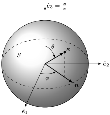
Figure 1: The unit sphere in Fourier space. The unit vector $\bm{\kappa}(\theta,\phi)$ is defined by the azimuth angle $\phi$, and the zenith angle $\theta$ measured from the axis $\hat{\bm{e}}_{3}=\bm{x}/x$.

Next, Eq. (36) is further simplified noting that the integration kernel is an even function of $\bm{\kappa}$. Therefore, the integral over the unit sphere $\mathcal{S}$ is twice the integral over a hemisphere.

At the origin, any arbitrary hemisphere $\mathcal{H}$ can be chosen, and the Green tensor assumes the value

$$\bm{G}(\bm{0}) =\frac{1}{8\pi^{2}}\int_{\mathcal{H}}\bm{\mathcal{C}}^{-\frac{1}{2}}(\bm{\kappa})\,\bm{\Lambda}^{-1}(\bm{\kappa})\,\bm{\mathcal{C}}^{-\frac{1}{2}}(\bm{\kappa})\text{d}\omega\,.$$ (37)

This noteworthy result shows that the Green tensor is non-singular at the origin, in contrast to classical elasticity.

Away from the origin, we can choose the hemisphere having the direction $\bm{x}$ as the zenith. This is a convenient choice because all points $\bm{\kappa}$ on such a hemisphere satisfy the condition $\bm{\kappa}\cdot\bm{x}\geq 0$. This hemisphere can be parameterized by the zenith angle $\theta$ and the azimuth angle $\phi$, as shown in Fig. 1. In this reference system, the unit vector $\bm{\kappa}$ can be expressed as

$$\bm{\kappa}(\theta,\phi)=\sin\theta\cos\phi\,\hat{\bm{e}}_{1}+\sin\theta\sin\phi\,\hat{\bm{e}}_{2}+\cos\theta\,\hat{\bm{e}}_{3}\,,$$ (38)

where $\hat{\bm{e}}_{3}=\bm{x}/x$. Finally, letting $q=\cos\theta$, the elementary solid angle becomes

$$\text{d}\omega=\sin\theta\,\text{d}\theta\,\text{d}\phi=-\text{d}q\,\text{d}\phi\,,$$ (39)

and

$$\bm{\kappa}(q,\phi)=\sqrt{1-q^{2}}\cos\phi\,\hat{\bm{e}}_{1}+\sqrt{1-q^{2}}\sin\phi\,\hat{\bm{e}}_{2}+q\,\hat{\bm{e}}_{3}\,.$$ (40)

Therefore the Green tensor of the anisotropic Mindlin differential operator of first order finally becomes

$${\bm{G}}(\bm{x})=\frac{1}{8\pi^{2}}\int_{0}^{2\pi}\int_{0}^{1} \bm{\mathcal{C}}^{-\frac{1}{2}}(\bm{\kappa})\exp\left\{-qx\,\bm{\Lambda}^{-1}(\bm{\kappa})\right\}\,\bm{\Lambda}^{-1}(\bm{\kappa})\,\bm{\mathcal{C}}^{-\frac{1}{2}}(\bm{\kappa})\,\text{d}q\,\text{d}\phi\,.$$ (41)

3.1 The first two gradients of the Green tensor

The first two gradients of the Green tensor are computed directly by differentiation of (36). The first gradient reads

$$\bm{\nabla}\bm{G}(\bm{x})=-\frac{1}{16\pi^{2}}\int_{\mathcal{S}} \bm{\mathcal{C}}^{-\frac{1}{2}}(\bm{\kappa})\exp\left\{-|\bm{\kappa}\cdot\bm{x}|\,\bm{\Lambda}^{-1}(\bm{\kappa})\right\}\,\bm{\Lambda}^{-2}(\bm{\kappa})$$

$$\times\bm{\mathcal{C}}^{-\frac{1}{2}}(\bm{\kappa})\otimes\bm{\kappa}\,\text{sign}(\bm{\kappa}\cdot\bm{x})\,\text{d}\omega\,.$$ (42)

In components this is:

$$G_{ij,m}(\bm{x})=-\frac{1}{16\pi^{2}}\int_{\mathcal{S}} \left[\bm{\mathcal{C}}^{-\frac{1}{2}}(\bm{\kappa})\exp\left\{-|\bm{\kappa}\cdot\bm{x}|\,\bm{\Lambda}^{-1}(\bm{\kappa})\right\}\,\bm{\Lambda}^{-2}(\bm{\kappa})\right.$$

$$\times\left.\bm{\mathcal{C}}^{-\frac{1}{2}}(\bm{\kappa})\right]_{ij}\kappa_{m}\,\text{sign}(\bm{\kappa}\cdot\bm{x})\,\text{d}\omega\,.$$ (43)

Note that, because of the presence of the sign function, the gradient of the Green tensor is finite but discontinuous at the origin. From a computational perspective, it is more convenient to express this result in reference system of Fig. 1. Doing so we find the alternative representation

$$G_{ij,m}(\bm{x})=-\frac{1}{8\pi^{2}}\int_{0}^{2\pi}\int_{0}^{1} \left[\bm{\mathcal{C}}^{-\frac{1}{2}}(\bm{\kappa})\exp\left\{-|\bm{\kappa}\cdot\bm{x}|\,\bm{\Lambda}^{-1}(\bm{\kappa})\right\}\,\bm{\Lambda}^{-2}(\bm{\kappa})\right.$$

$$\left.\bm{\mathcal{C}}^{-\frac{1}{2}}(\bm{\kappa})\right]_{ij}\kappa_{m}\,\text{d}q\,\,\text{d}\phi.$$ (44)

The second gradient of the Green tensor reads

$$\bm{\nabla}\bm{\nabla}\bm{G}(\bm{x}) =\frac{1}{16\pi^{2}}\int_{\mathcal{S}}\Big{(}\bm{\mathcal{C}}^{-\frac{1}{2}}(\bm{\kappa})\exp\left\{-|\bm{\kappa}\cdot\bm{x}|\,\bm{\Lambda}^{-1}(\bm{\kappa})\right\}\,$$

$$\hskip 56.9055pt\times\bm{\Lambda}^{-3}(\bm{\kappa})\,\bm{\mathcal{C}}^{-\frac{1}{2}}(\bm{\kappa})\otimes\bm{\kappa}\otimes\bm{\kappa}$$

$$\ -\bm{\mathcal{C}}^{-\frac{1}{2}}(\bm{\kappa})\,\bm{\Lambda}^{-2}(\bm{\kappa})\,\bm{\mathcal{C}}^{-\frac{1}{2}}(\bm{\kappa})\otimes\bm{\kappa}\otimes\bm{\kappa}\,\delta(\bm{\kappa}\cdot\bm{x})\Big{)}\,\text{d}\omega\,.$$ (45)

Letting $\bm{n}(\phi)=\bm{\kappa}(\pi/2,\phi)$ be a unit vector on the equatorial plane $\bm{\kappa}\cdot\bm{x}=0$, we finally obtain

$$\bm{\nabla}\bm{\nabla}\bm{G}(\bm{x}) =\frac{1}{16\pi^{2}}\int_{\mathcal{S}}\bm{\mathcal{C}}^{-\frac{1}{2}}(\bm{\kappa})\exp\left\{-|\bm{\kappa}\cdot\bm{x}|\,\bm{\Lambda}^{-1}(\bm{\kappa})\right\}\,$$

$$\hskip 56.9055pt\times\bm{\Lambda}^{-3}(\bm{\kappa})\,\bm{\mathcal{C}}^{-\frac{1}{2}}(\bm{\kappa})\otimes\bm{\kappa}\otimes\bm{\kappa}\,\text{d}\omega\,$$

$$\ -\frac{1}{8\pi^{2}x}\int_{0}^{2\pi}\bm{\mathcal{C}}^{-\frac{1}{2}}(\bm{n})\,\bm{\Lambda}^{-2}(\bm{n})\,\bm{\mathcal{C}}^{-\frac{1}{2}}(\bm{n})\otimes\bm{n}\otimes\bm{n}\,\text{d}\phi\,.$$ (46)

Note that the second gradient of the Green tensor is singular at the origin.

3.2 The classical limit

It is now shown that Green tensor (36) converges to the classical Green tensor $\bm{G}^{0}$ Lifshitz and Rosenzweig (1947); Synge (1957) when the field point $\bm{x}$ is sufficiently far from the origin compared to the characteristic length scales, that is when

$$|\bm{\kappa}\cdot\bm{x}|/\lambda_{i}\gg 1,$$ (47)

where $\lambda_{i}$ is an eigenvalue of $\bm{\Lambda}$, and $i=1,2,3$. This important property guarantees that the non-singular Green tensor (41) regularizes the classical anisotropic Green tensor in the far field. Moreover, as a special case satisfying condition (47), the classical Green tensor $\bm{G}^{0}$ is also recovered in the limit of vanishing tensor of strain gradient coefficients $\mathbb{D}$. The classical Green tensor $\bm{G}^{0}$ is readily recovered if we consider the limit

$$\lim_{\||\bm{\kappa}\cdot\bm{x}|\,\bm{\Lambda}^{-1}\|\rightarrow\infty}\,\exp\left\{-|\bm{\kappa}\cdot\bm{x}|\,\bm{\Lambda}^{-1}(\bm{\kappa})\right\}\,\bm{\Lambda}^{-1}(\bm{\kappa})=\frac{2\bm{I}}{x}\,\delta(\bm{\kappa}\cdot\hat{\bm{x}})\,,$$ (48)

where $\hat{\bm{x}}=\bm{x}/x$ and $\bm{I}$ is the identity tensor. In fact, the substitution of (48) into (36) yields

$$\bm{G}(\bm{x})\rightarrow\bm{G}^{0}(\bm{x}) =\frac{1}{8\pi^{2}x}\int_{\mathcal{S}}\bm{\mathcal{C}}^{-1}(\bm{\kappa})\,\delta(\bm{\kappa}\cdot\bm{x})\,\text{d}\omega=\frac{1}{8\pi^{2}x}\,\int_{0}^{2\pi}\bm{\mathcal{C}}^{-1}(\bm{n})\,\text{d}\phi\,.$$ (49)

Here we used again the notation $\bm{n}(\phi)=\bm{\kappa}(\pi/2,\phi)$ to indicate a unit vector on the equatorial plane $\bm{\kappa}\cdot\bm{x}=0$. Note that the span of integration can be reduced to the range $0\leq\phi\leq\pi$ using the symmetry $\bm{\mathcal{C}}^{-1}(\bm{n})=\bm{\mathcal{C}}^{-1}(-\bm{n})$.

4 Special cases

In this section we show that the Green tensor (36) generalizes other results obtained in the literature.

4.1 The weakly non-local Green tensor $\mathbf{G}^{\text{NL}}$

Lazar and Po Lazar and Po (2015) have considered a simplified strain gradient elasticity theory under the assumption

$$\mathbb{D}_{ijmkln}=\mathbb{C}_{ijkl}{L}_{mn}\,,$$ (50)

a framework which was named Mindlin’s strain gradient elasticity with weak non-locality because of its relation to non-local theories Lazar et al (2018); Lazar and Agiasofitou (2011). The Green tensor (36) recovers our previous result as a special case. In fact, under the previous assumption, we have

$$\bm{\Lambda}(\bm{\kappa})=\bm{I}\,\sqrt{\bm{\kappa}^{T}\bm{L}\bm{\kappa}}\,,$$ (51)

and

$$\exp\left\{-|\bm{\kappa}\cdot\bm{x}|\,\bm{\Lambda}^{-1}(\bm{\kappa})\right\}\,\bm{\Lambda}^{-1}(\bm{\kappa})=\bm{I}\frac{\exp\left(-\frac{|\bm{\kappa}\cdot\bm{x}|}{\sqrt{\bm{\kappa}^{T}\bm{L}\bm{\kappa}}}\right)}{\sqrt{\bm{\kappa}^{T}\bm{L}\bm{\kappa}}}\,.$$

Therefore the Green tensor becomes

$$\bm{G}^{\text{NL}}(\bm{R}) =\frac{1}{16\pi^{2}}\int_{\mathcal{S}}\bm{\mathcal{C}}^{-1}(\bm{\kappa})\frac{\exp\left(-\frac{|\bm{\kappa}\cdot\bm{x}|}{\sqrt{\bm{\kappa}^{T}\bm{L}\bm{\kappa}}}\right)}{\sqrt{\bm{\kappa}^{T}\bm{L}\bm{\kappa}}}\,\text{d}\omega\,,$$ (52)

which is the expression given in Lazar and Po (2015).

4.2 The Green tensor of anisotropic gradient elasticity of Helmholtz type $\mathbf{G}^{\text{H}}$

An even simpler theory, named Mindlin’s gradient elasticity of Helmholtz type, has been proposed by Lazar and Po (2015). The theory is characterized by only one gradient length scale parameter $\ell$, which renders the tensor $\bm{L}$ diagonal:

$$\bm{L}=\ell^{2}\,\bm{I}\,.$$ (53)

The non-singular Green tensor of this theory is obtained by substituting (53) in (52), thus yielding

$$\bm{G}^{\text{H}}(\bm{R}) =\frac{1}{16\pi^{2}\ell}\int_{\mathcal{S}}\bm{\mathcal{C}}^{-1}(\bm{\kappa})\exp\left(-\frac{|\bm{\kappa}\cdot\bm{x}|}{\ell}\right)\,\text{d}\omega\,,$$ (54)

which coincides with the expression given in Lazar and Po (2015).

4.3 The isotropic Green tensor $\mathbf{G}^{\text{I}}$

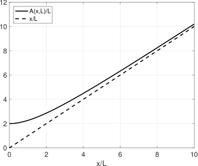
Figure 2: Plot of the regularized distance function $A(x,\ell)$.

The isotropic tensor $\mathbb{C}$ has components

$$\mathbb{C}_{ijkl}=\lambda\delta_{ij}\delta_{kl}+\mu\big{(}\delta_{ik}\delta_{jl}+\delta_{il}\delta_{jk}\big{)}\,,$$ (55)

where $\lambda$ and $\mu$ are the Lamé constants. On the other hand, the isotropic tensor $\mathbb{D}$ reads

$$\mathbb{D}_{ijmkln} =\frac{a_{1}}{2}\big{(}\delta_{ij}\delta_{km}\delta_{ln}+\delta_{ij}\delta_{kn}\delta_{lm}+\delta_{kl}\delta_{im}\delta_{jn}+\delta_{kl}\delta_{in}\delta_{jm}\big{)}$$

$$\ +\frac{a_{3}}{2}\big{(}\delta_{jk}\delta_{im}\delta_{kl}+\delta_{ik}\delta_{jm}\delta_{nl}+\delta_{il}\delta_{jm}\delta_{kn}+\delta_{jl}\delta_{im}\delta_{kn}\big{)}$$

$$\ +\frac{a_{5}}{2}\big{(}\delta_{jk}\delta_{in}\delta_{lm}+\delta_{ik}\delta_{jn}\delta_{lm}+\delta_{jl}\delta_{km}\delta_{in}+\delta_{il}\delta_{km}\delta_{jn}\big{)}$$

$$\ +2a_{2}\,\delta_{ij}\delta_{kl}\delta_{mn}+a_{4}\big{(}\delta_{il}\delta_{jk}\delta_{mn}+\delta_{ik}\delta_{jl}\delta_{mn}\big{)}\,,$$ (56)

where $a_{1}$, $a_{2}$, $a_{3}$, $a_{4}$, $a_{5}$ are the gradient parameters in isotropic Mindlin’s first strain gradient elasticity theory Mindlin (1964) (see also Mindlin (1968); Lazar and Po (2018)). Therefore, the matrices $\bm{\mathcal{C}}(\bm{\kappa})$ and $\bm{\mathcal{D}}(\bm{\kappa})$ become, respectively

$$\mathcal{C}_{ik}(\bm{\kappa}) =(\lambda+2\mu)\kappa_{i}\kappa_{k}+\mu\big{(}\delta_{ik}-\kappa_{i}\kappa_{k}\big{)}\,,$$ (57)

$$\mathcal{D}_{ik}(\bm{\kappa}) =2(a_{1}+a_{2}+a_{3}+a_{4}+a_{5})\kappa_{i}\kappa_{k}$$

$$\ +\frac{1}{2}\,(a_{3}+2a_{4}+a_{5})\big{(}\delta_{ik}-\kappa_{i}\kappa_{k}\big{)}$$

$$=(\lambda+2\mu)\,\ell_{1}^{2}\kappa_{i}\kappa_{k}+\mu\,\ell_{2}^{2}\big{(}\delta_{ik}-\kappa_{i}\kappa_{k}\big{)}\,.$$ (58)

The two characteristic lengths $\ell_{1}$ and $\ell_{2}$ introduced above are defined as

$$\ell_{1}^{2} =\frac{2(a_{1}+a_{2}+a_{3}+a_{4}+a_{5})}{\lambda+2\mu}\,,$$ (59)

$$\ell_{2}^{2} =\frac{a_{3}+2a_{4}+a_{5}}{2\mu}\,.$$ (60)

Owing to the special structure of $\bm{\mathcal{C}}(\bm{\kappa})$ and $\bm{\mathcal{D}}(\bm{\kappa})$, the following results are easily obtained:

$$\mathcal{C}^{-\frac{1}{2}}_{ij}(\bm{\kappa}) =\frac{1}{\sqrt{\mu}}\left(\delta_{ij}-\kappa_{i}\kappa_{j}\right)-\frac{1}{\sqrt{\lambda+2\mu}}\kappa_{i}\kappa_{j}$$ (64)

$$\Lambda_{ij}^{-1}(\bm{\kappa}) =\frac{1}{\ell_{2}}\left(\delta_{ij}-\kappa_{i}\kappa_{j}\right)+\frac{1}{\ell_{1}}\kappa_{i}\kappa_{j}\,.$$ (65)

The matrix $\bm{\Lambda}^{-1}$ admits the eigenvalue $1/\ell_{1}$, corresponding to the eigenvector $\hat{\bm{v}}_{1}=\bm{\kappa}$. The degenerate eigenvalue $1/\ell_{2}$ has multiplicity two, corresponding to two arbitrary eigenvectors $\hat{\bm{v}}_{2}$ and $\hat{\bm{v}}_{3}$ perpendicular to $\bm{\kappa}$. Choosing such eigenvectors to be mutually orthogonal, the matrix $\bm{\Lambda}^{-1}$ admits the eigen decomposition $\bm{\Lambda}^{-1}=\bm{Q}\bm{D}^{-1}\bm{Q}^{T}$. Here

$$\bm{Q}=[\hat{\bm{v}}_{1}\,\hat{\bm{v}}_{2}\,\hat{\bm{v}}_{3}]$$ (66)

is an orthogonal matrix whose columns are the eigenvectors of $\bm{\Lambda}^{-1}$, and

$$\bm{D}^{-1}=\text{diag}\left\{\frac{1}{\ell_{1}},\,\frac{1}{\ell_{2}},\,\frac{1}{\ell_{2}}\right\}$$ (67)

is the diagonal matrix of its eigenvalues. This special form of $\bm{Q}$ yields the identity

$$\bm{\mathcal{C}}^{-\frac{1}{2}}\bm{Q}=\bm{Q}\,\text{diag}\left\{-\frac{1}{\sqrt{\lambda+2\mu}},\,\frac{1}{\sqrt{\mu}},\,\frac{1}{\sqrt{\mu}}\right\}\,.$$ (68)

Using these results in (36), we obtain

$$\bm{G}^{I}(\bm{x}) =\frac{1}{16\pi^{2}}\int_{\mathcal{S}}\bm{\mathcal{C}}^{-\frac{1}{2}}\bm{Q}\exp\left\{-|\bm{\kappa}\cdot\bm{x}|\,\bm{D}^{-1}\right\}\,\bm{D}^{-1}\bm{Q}^{T}\bm{\mathcal{C}}^{-\frac{1}{2}}\text{d}\omega$$

$$=\frac{1}{16\pi^{2}}\int_{\mathcal{S}}\bm{Q}\,\text{diag}\left\{\frac{e^{\frac{-|\bm{\kappa}\cdot\bm{x}|}{\ell_{1}}}}{\ell_{1}(\lambda+2\mu)},\,\frac{e^{\frac{-|\bm{\kappa}\cdot\bm{x}|}{\ell_{2}}}}{\ell_{2}\mu},\,\frac{e^{\frac{-|\bm{\kappa}\cdot\bm{x}|}{\ell_{2}}}}{\ell_{2}\mu}\right\}\bm{Q}^{T}\text{d}\omega$$

$$=\frac{1}{16\pi^{2}}\int_{\mathcal{S}}\frac{e^{\frac{-|\bm{\kappa}\cdot\bm{x}|}{\ell_{1}}}}{(\lambda+2\mu)\ell_{1}}\hat{\bm{v}}_{1}\otimes\hat{\bm{v}}_{1}\text{d}\omega$$

$$+\frac{1}{16\pi^{2}}\int_{\mathcal{S}}\frac{e^{\frac{-|\bm{\kappa}\cdot\bm{x}|}{\ell_{2}}}}{\mu\ell_{2}}\left(\hat{\bm{v}}_{2}\otimes\hat{\bm{v}}_{2}+\hat{\bm{v}}_{3}\otimes\hat{\bm{v}}_{3}\right)\text{d}\omega\,.$$ (69)

Because they form an orthonormal basis, the three eigenvectors satisfy the identity $\hat{\bm{v}}_{1}\otimes\hat{\bm{v}}_{1}+\hat{\bm{v}}_{2}\otimes\hat{\bm{v}}_{2}+\hat{\bm{v}}_{3}\otimes\hat{\bm{v}}_{3}=\bm{I}$, hence we have

$$\bm{G}^{I}(\bm{x}) =\frac{1}{16\pi^{2}}\int_{\mathcal{S}}\left[\frac{e^{\frac{-|\bm{\kappa}\cdot\bm{x}|}{\ell_{1}}}}{(\lambda+2\mu)\ell_{1}}{\bm{\kappa}}\otimes{\bm{\kappa}}+\frac{e^{\frac{-|\bm{\kappa}\cdot\bm{x}|}{\ell_{2}}}}{\mu\ell_{2}}\left(\bm{I}-{\bm{\kappa}}\otimes{\bm{\kappa}}\right)\right]\text{d}\omega\,.$$ (70)

The integral over the unit sphere is carried out using the relation

$$\int_{\mathcal{S}}\frac{e^{\frac{-|\bm{\kappa}\cdot\bm{x}|}{\ell}}}{\ell}\kappa_{i}\kappa_{j}\,\text{d}\omega=2\pi\,\partial_{i}\partial_{j}A(x,\ell)\,,$$ (71)

where the scalar function $A(x,\ell)$ is

$$A(x,\ell)=x+\frac{2\ell^{2}}{x}-\frac{2\ell^{2}}{x}e^{-x/\ell}\,.$$ (72)

The scalar function $A(x,\ell)$ can be regarded as a regularized distance function in the sense that $A(x,\ell)$ tends to $x$ when $x/\ell\gg 1$, while it smoothly approaches to $2\ell$ for small $x$, as shown in Fig. 2. By sake of (71), the Green tensor finally becomes:

$$G_{ij}(\bm{x})=\frac{1}{8\pi\mu}\,\Big{[}\frac{\mu}{\lambda+2\mu}\,\partial_{i}\partial_{j}A(x,\ell_{1})+\big{(}\delta_{ij}\Delta-\partial_{i}\partial_{j}\big{)}A(x,\ell_{2})\Big{]}\,.$$ (73)

This result can also be obtained by direct inverse Fourier transform of (26), as shown in Appendix A. A more detailed analysis of the isotropic Green tensor (73) can be found in Lazar and Po (2018).

5 A comparison with Molecular Statics: The Kelvin problem

	Cu EAM	Cu MEAM	Al MEAM
${C}_{1,1}$ $[\text{eV}/\textup{\AA}^{3}]$	1.0868	1.0994	7.1366$\cdot 10^{-1}$
${C}_{1,2}$ $[\text{eV}/\textup{\AA}^{3}]$	7.9386$\cdot 10^{-1}$	7.7973$\cdot 10^{-1}$	3.8649$\cdot 10^{-1}$
${C}_{4,4}$ $[\text{eV}/\textup{\AA}^{3}]$	5.2252$\cdot 10^{-1}$	5.1043$\cdot 10^{-1}$	1.9704$\cdot 10^{-1}$
${D}_{1,1}$ $[\text{eV}/\textup{\AA}]$	1.1182	6.5018$\cdot 10^{-1}$	1.0855
${D}_{1,2}$ $[\text{eV}/\textup{\AA}]$	3.5814$\cdot 10^{-1}$	3.6659$\cdot 10^{-1}$	1.4572$\cdot 10^{-1}$
${D}_{1,3}$ $[\text{eV}/\textup{\AA}]$	3.7951$\cdot 10^{-1}$	2.4150$\cdot 10^{-1}$	1.5934$\cdot 10^{-1}$
${D}_{2,2}$ $[\text{eV}/\textup{\AA}]$	4.7935$\cdot 10^{-1}$	7.3885$\cdot 10^{-1}$	8.4221$\cdot 10^{-1}$
${D}_{2,3}$ $[\text{eV}/\textup{\AA}]$	3.0103$\cdot 10^{-1}$	2.0651$\cdot 10^{-1}$	1.5671$\cdot 10^{-1}$
${D}_{2,4}$ $[\text{eV}/\textup{\AA}]$	1.2789$\cdot 10^{-1}$	4.7496$\cdot 10^{-1}$	7.1708$\cdot 10^{-1}$
${D}_{2,5}$ $[\text{eV}/\textup{\AA}]$	1.0652$\cdot 10^{-1}$	-4.2545$\cdot 10^{-2}$	-1.1434$\cdot 10^{-2}$
${D}_{3,3}$ $[\text{eV}/\textup{\AA}]$	4.3662$\cdot 10^{-1}$	2.9055$\cdot 10^{-1}$	2.7613$\cdot 10^{-1}$
${D}_{3,5}$ $[\text{eV}/\textup{\AA}]$	1.2789$\cdot 10^{-1}$	-1.8275$\cdot 10^{-2}$	-1.2408$\cdot 10^{-1}$
${D}_{16,16}$ $[\text{eV}/\textup{\AA}]$	1.4925$\cdot 10^{-1}$	3.7419$\cdot 10^{-2}$	1.6786$\cdot 10^{-1}$
${D}_{16,17}$ $[\text{eV}/\textup{\AA}]$	1.0652$\cdot 10^{-1}$	3.7394$\cdot 10^{-2}$	1.5006$\cdot 10^{-1}$

Table 1: Elastic and gradient-elastic constants obtained from the interatomic potentials Lee (2001) and Mendelev (2008).

In this section, we compare the Green tensor obtained from Mindlin’s strain gradient elastic theory to that obtained from an atomistic system. This study was carried out using Minimol Tadmor and Miller (2011) which is a KIM-compliant molecular dynamics (MD) and molecular statics (MS) program. The Open Knowledgebase of Interatomic Models (KIM) is a project focused on creating standards for atomistic simulations including an application programming interface (API) for information exchange between atomistic simulation codes and interatomic potentials Tadmor et al. (2011, 2013).

(a) $\mathbb{C}$ for Cu EAM

(b) $\mathbb{C}$ for Cu MEAM

(c) $\mathbb{C}$ for Al MEAM

(d) $\mathbb{D}$ for Cu EAM

(e) $\mathbb{D}$ for Cu MEAM

(f) $\mathbb{D}$ for Al MEAM

Figure 3: Voigt representation of the elastic tensors $\mathbb{C}$ and gradient-elastic tensor $\mathbb{D}$ for fcc Al and Cu, computed from the interatomic potentials Lee (2001) and Mendelev (2008). LABEL:sub@C_Cu_fcc_EAM_Mendelev_2013 and LABEL:sub@D_Cu_fcc_EAM_Mendelev_2013 Cu for EAM potential Mendelev (2008). LABEL:sub@C_Cu_fcc_MEAM_Lee_2001 and LABEL:sub@D_Cu_fcc_MEAM_Lee_2001 Cu for MEAM potential Lee (2001). LABEL:sub@C_Al_fcc_MEAM_Lee_2001 and LABEL:sub@D_Al_fcc_MEAM_Lee_2001 Al for MEAM potential Lee (2001).

We choose face-centered-cubic Aluminum and Copper for this comparison, and consider the following two interatomic potentials: the modified-embedded-atom-method (MEAM) by Lee (2001), and the embedded-atom-potential by Mendelev et al. (2008), which are archived in the OpenKIM repository. Elastic and gradient-elastic constants for these potentials were computed using the method described in Admal et al (2016), and they are available on the KIM repository Lee (2001); Mendelev (2008). For convenience, the values of the independent elastic and gradient-elastic constants are reported in table 1. These components are used to populate the elastic tensors $\mathbb{C}$ and $\mathbb{D}$ Admal et al (2016); Auffray et al. (2013). The Voigt structure of the resulting tensors $\mathbb{C}$ and $\mathbb{D}$ is shown in Fig. 3.

The atomistic system is constructed by stacking together $15\times 15\times 15$ unit cells resulting in $13500$ atoms. A force of $0.0116$ eV/Å in the $x_{1}$ direction is imposed on the central atom of the system, and displacement boundary conditions are imposed on five layers of atoms close to the boundary using the classical solution given in Eq. (49). The padding atoms thickness is 0.15 times the size of the box. A MS simulation is carried out using the above-mentioned boundary conditions resulting in a deformed crystal. The resulting displacement field normalized with respect to the force on the central atom yields the atomistic Green tensor component fields.

Simulation results are shown in Fig. 4, where we compare the Green tensor components $G_{11}(x_{1},0,0)$ and $G_{22}(x_{1},0,0)$. Despite the fact that these potentials were never fitted to gradient-elastic constants, it can be observed that the analytical predictions are in good agreement with MS calculations, with a maximum error at the origin in the order of 5-30%, depending on the potential used. It should be noted that, compared to the EAM potential, the MEAM potential better compares to the analytical results, possibly as a result of artifacts in gradient-elastic constants evaluated by EAM potentials Admal et al (2016).

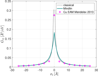
(a) Cu EAM

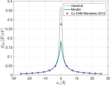
(b) Cu EAM

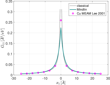
(c) Cu MEAM

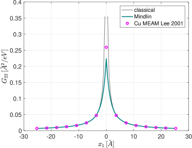
(d) Cu MEAM

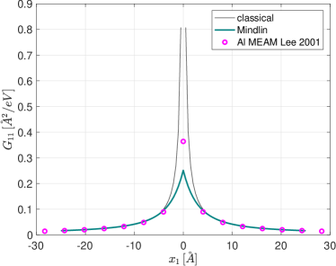
(e) Al MEAM

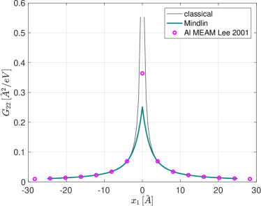
(f) Al MEAM

Figure 4: Components of the Green tensor for fcc Al and Cu, and comparison to atomistic calculations obtained from the interatomic potentials Lee (2001) and Mendelev (2008). LABEL:sub@Cu_fcc_EAM_Mendelev_2013_G_11_x1-LABEL:sub@Cu_fcc_EAM_Mendelev_2013_G_22_x1 Cu for EAM potential Mendelev (2008). LABEL:sub@Cu_fcc_MEAM_Lee_2001_G_11_x1-LABEL:sub@D_Cu_fcc_MEAM_Lee_2001 Cu for MEAM potential Lee (2001). LABEL:sub@Al_fcc_MEAM_Lee_2001_G_11_x1-LABEL:sub@Al_fcc_MEAM_Lee_2001_G_22_x1 Al for MEAM potential Lee (2001).

6 Summary and Conclusions

In this paper we have derived an expression for the Green tensor of Mindlin’s anisotropic strain gradient elasticity, which possesses up to 21 elastic constants and 171 gradient elastic constants in the general case of triclinic media. The Green tensor is found in terms of a matrix kernel integrated over the unit sphere in Fourier space. Such representation is similar to that of the classical anisotropic Green tensor, which requires integration over the equatorial plane of the unit sphere. In contrast to its classical counterpart, however, the Green tensor of Mindlin’s anisotropic strain gradient elasticity is non-singular at the origin, while its gradient is finite but discontinuous at the origin. It is shown that the non-singular Green tensor converges to the classical tensor a few characteristic lengths away from the origin. Therefore, the Green tensor of Mindlin’s first strain gradient elasticity can be regarded as a physical regularization of the classical anisotropic Green tensor. Moreover, existing expressions of the Green tensor found in the literature are recovered as special cases. Because the Green tensor regularizes its classical counterpart without unphysical singularities, it offers a more realistic description of near-core elastic fields of defects in micro-mechanics, and it provides more accurate boundary conditions for atomistic and ab-initio energy-minimization calculations. As an illustrative example, we have computed the displacement field induced by a concentrated force acting at the origin (Kelvin problem), and compared the analytical predictions to atomistic calculations when the elastic and gradient-elastic moduli are consistently derived from the interatomic potentials. Despite the fact that these potentials were not fitted to gradient-elastic constants, it is shown that the analytical predictions are in good agreement with MS calculations, with a maximum error at the origin in the order of 5-30%, depending on the potential used.

List of Abbreviations

PDE: partial differential equation. SPD: symmetric positive definite. KIM: Open Knowledgebase of Interatomic Models. API: application programming interface. EAM: embedded atom method. MEAM: modified embedded atom method.

Declarations

Availability of data and materials. Elastic and gradient-elastic material constants used to obtain the results in section 5 are freely available as part of the Open Knowledgebase of Interatomic Models (KIM).

Competing Interest. The authors declare that they have no competing interests.

Funding. G.P. acknowledges the support of the U.S. Department of Energy, Office of Fusion Energy, through the DOE award number DE-SC0018410, the Air Force Office of Scientific Research (AFOSR), through award number FA9550-16-1-0444, and the National Science Foundation, Division of Civil, Mechanical and Manufacturing Innovation (CMMI), through award number 1563427 with UCLA. N.A. acknowledges the support of the US Department of Energy’s Office of Fusion Energy Sciences, Grant No. DE-SC0012774:0001. M.L. gratefully acknowledges a grant from the Deutsche Forschungsgemeinschaft (Grant No. La1974/4-1).

Authors Contribution. G.P. and M.L. obtained the expression of the Green Tensor. N.A. and G.P. carried out the numerical analysis. All authors read and approved the final manuscript.

Appendix A Direct derivation of Mindlin’s isotropic strain gradient elasticity of form II

Plugging (57) and (58) into (26) we have

$$\bm{G}(\bm{k}) =\frac{\left[\left(\lambda+2\mu\right)\left(1+k^{2}\ell_{1}^{2}\right)\bm{\kappa}\otimes\bm{\kappa}+\mu\left(1+k^{2}\ell_{2}^{2}\right)\left(\bm{I}-\bm{\kappa}\otimes\bm{\kappa}\right)\right]^{-1}}{k^{2}}\,.$$ (74)

Owing to its special structure (see footnote 6), the matrix in the numerator can be easily inverted. In index notation the result is

$$G_{ij}(\bm{k}) =\frac{\kappa_{i}\kappa_{j}}{\left(\lambda+2\mu\right)k^{2}\left(1+k^{2}\ell_{1}^{2}\right)}+\frac{\delta_{ij}-\kappa_{i}\kappa_{j}}{\mu k^{2}\left(1+k^{2}\ell_{1}^{2}\right)}$$

$$=\frac{k_{i}k_{j}}{\left(\lambda+2\mu\right)k^{4}\left(1+k^{2}\ell_{1}^{2}\right)}+\frac{k^{2}\delta_{ij}-k_{i}k_{j}}{\mu k^{4}\left(1+k^{2}\ell_{1}^{2}\right)}\,.$$ (75)

Using the the general form of the Fourier transform of the derivative, the Green tensor in real space is obtained as

$$G_{ij}(\bm{x}) =-\frac{\partial_{i}\partial_{j}}{\lambda+2\mu}\mathcal{F}^{-1}\left[\frac{1}{k^{4}\left(1+k^{2}\ell_{1}^{2}\right)}\right]-\frac{\delta_{ij}\Delta-\partial_{i}\partial_{j}}{\mu}\mathcal{F}^{-1}\left[\frac{1}{k^{4}\left(1+k^{2}\ell_{1}^{2}\right)}\right]\,.$$ (76)

Now consider the identity

$$\mathcal{F}^{-1}\left[\frac{1}{k^{4}\left(1+k^{2}\ell^{2}\right)}\right] =\mathcal{F}^{-1}\left[\frac{1}{k^{4}}-\frac{\ell^{2}}{k^{2}}+\frac{\ell^{4}}{1+k^{2}\ell_{1}^{2}}\right]=-\frac{1}{8\pi}\left(x+\frac{2\ell^{2}}{x}-\frac{2\ell^{2}}{x}e^{-x/\ell}\right)$$

$$=-\frac{1}{8\pi}A(x,\ell)\,.$$ (77)

Using (77) in (76), the Green tensor (73) is readily recovered.

List of Figures

1. 1 The unit sphere in Fourier space. The unit vector $\bm{\kappa}(\theta,\phi)$ is defined by the azimuth angle $\phi$, and the zenith angle $\theta$ measured from the axis $\hat{\bm{e}}_{3}=\bm{x}/x$.
2. 2 Plot of the regularized distance function $A(x,\ell)$.
3. 3 Voigt representation of the elastic tensors $\mathbb{C}$ and gradient-elastic tensor $\mathbb{D}$ for fcc Al and Cu, computed from the interatomic potentials Lee (2001) and Mendelev (2008). and Cu for EAM potential Mendelev (2008). and Cu for MEAM potential Lee (2001). and Al for MEAM potential Lee (2001).
4. 4 Components of the Green tensor for fcc Al and Cu, and comparison to atomistic calculations obtained from the interatomic potentials Lee (2001) and Mendelev (2008). - Cu for EAM potential Mendelev (2008). - Cu for MEAM potential Lee (2001). - Al for MEAM potential Lee (2001).

References

- Green (1828) Green, G., 1828. An Essay on the Application of Mathematical Analysis to the Theories of Electricity and Magnetism. Nottingham (the author).
- Becker (1992) Becker, A.A., 1992. The Boundary Element Method in Engineering: A Complete Course.. Mcgraw-Hill.
- Trinkle (2008) D. R. Trinkle. Lattice Green function for extended defect calculations: Computation and error estimation with long-range forces. Phys. Rev. B 78 (2008), 014110
- Lord Kelvin (1882) Lord Kelvin, 1882. Mathematical and Physical Papers, Vol. 1. Cambridge University Press, Cambridge, p. 97.
- Lifshitz and Rosenzweig (1947) I.M. Lifshitz, L.N. Rosenzweig, On the construction of the Green tensor for the basic equation of the theory of elasticity of an anisotropic medium, Zh. Eksper. Teor. Fiz. 17 (1947) 783–791.
- Synge (1957) J.L. Synge, The Hypercircle in Mathematical Physics, Cambridge University Press, Cambridge, 1957.
- Barnett (1972) D.M. Barnett, The precise evaluation of derivatives of the anisotropic elastic Green functions, phys. stat. sol. (b) 49 (1972) 741–748.
- Bacon et al. (1979) D.J. Bacon, D.M. Barnett, R.O. Scattergood, Anisotropic continuum theory of defects, Prog. Mater. Sci. 23 (1979) 51–262.
- Teodosiu (1982) C. Teodosiu, Elastic Models of Crystal Defects, Springer, Berlin, 1982.
- Mura (1987) T. Mura, Micromechanics of Defects in Solids, 2nd edition, Martinus Nijhoff, Dordrecht, 1987.
- Askes and Aifantis (2011) H. Askes, E.C. Aifantis. Gradient elasticity in statics and dynamics: an overview of formul‘ations, length scale identification procedures, finite element implementations and new results. International Journal of Solids and Structures, 48(13) (2011), 1962-1990.
- Eringen (1999) A.C. Eringen. Microcontinuum field theories: I. Foundations and solids (1999). Springer Science & Business Media.
- Eringen (2002) A.C. Eringen. Nonlocal continuum field theories (2002). Springer Science & Business Media.
- Kröner (1963) Ekkehart Kröner. On the physical reality of torque stresses in continuum mechanics. Int J Engng Sci 1 (1963), 261-278.
- Mindlin (1964) R.D. Mindlin, Micro-structure in linear elasticity, Arch. Rational. Mech. Anal. 16 (1964) 51–78.
- Mindlin (1968) R.D. Mindlin, Theories of elastic continua and crystal lattice theories, In: Kröner, E. (Ed.), Mechanics of Generalized Continua, IUTAM Symposium, Springer, Berlin, 1968, pp. 312–320.
- Mindlin (1972) R.D. Mindlin, Elasticity, piezoelectricity and crystal lattice dynamics, J. Elast. 2 (1972) 217–282.
- Mindlin and Eshel (1968) R.D. Mindlin, N.N. Eshel. On first strain gradient theories in linear elasticity. Int J Solids Struct 4 (1968), 109-124.
- Polizzotto (2018) C. Polizzotto, Anisotropy in strain gradient elasticity: Simplified models with different forms of internal length and moduli tensors, European Journal of Mechanics-A/Solids, 71 (2018) 51–63.
- Auffray et al. (2013) N. Auffray, H. Le Quang, Q.C. He, Matrix representations for 3D strain gradient elasticity, J. Mech. Phys. Solids 61 (2013) 1202-1223.
- Admal et al (2016) N. C. Admal, J. Marian, G. Po. The atomistic representation of first strain gradient elastic tensors. Journal of the Mechanics and Physics of Solids, 99 (2016), 93-115.
- Rogula (1973) D. Rogula, Some basic solutions in strain gradient elasticity theory of an arbitrary order, Arch. Mech. 25 (1973), 43–68.
- Lazar and Po (2018) M. Lazar, G. Po, On Mindlin’s theory of strain gradient elasticity: Green tensors, regularization, and operator-split JMMP (accepted), https://doi.org/10.1142/S2424913018400088
- Lazar and Po (2015) M. Lazar, G. Po, The non-singular Green tensor of gradient anisotropic elasticity of Helmholtz type, Eur. J. Mech. A Solids 50 (2015) 152–162.
- Lazar and Po (2015) M. Lazar, G. Po, The non-singular Green tensor of Mindlin’s anisotropic gradient elasticity with separable weak non-locality, Physics Letters A 379 (2015), 1538–1543.
- Lazar et al (2018) Markus Lazar, Eleni Agiasofitou, Giacomo Po. Nonlocal anisotropic elasticity: fundamentals and application to three-dimensional dislocation problems.
- Lazar and Agiasofitou (2011) M Lazar, E Agiasofitou Screw dislocation in nonlocal anisotropic elasticity International Journal of Engineering Science 49 (2011), 1404-1414
- Vladimirov (1971) V.S. Vladimirov, Equations of Mathematical Physics, Marcel Dekker, Inc., New York, 1971.
- Lazar and Po (2018) M. Lazar, Irreducible decomposition of strain gradient tensor in isotropic strain gradient elasticity, Z. Angew. Math. Mech. 96 (2016), 1291–1305.
- Tadmor et al. (2011) Tadmor, E.B., Elliott, R.S., Sethna, J.P., Miller, R.E., Becker, C.A. The potential of atomistic simulations and the Knowledgebase of Interatomic Models. JOM 63 (2011), 17-17
- Tadmor et al. (2013) Tadmor, E.B., Elliott, R.S., Phillpot, S.R., Sinnott, S.B. NSF cyberinfrastructures: a new paradigm for advancing materials simulation. Curr. Opin. Solid State Mater. Sci. 17 (6) (2013), 298-304.
- Lee (2001) Lee, Byeong-Joo and Baskes, M.I. and Kim, Hanchul and Koo Cho, Yang. Second nearest-neighbor modified embedded atom method potentials for bcc transition metals. Phys. Rev. B, 64 (2001) 184102
- Mendelev et al. (2008) Mendelev, MI and Kramer, MJ and Becker, CA and Asta, M. Analysis of semi-empirical interatomic potentials appropriate for simulation of crystalline and liquid Al and Cu. Philosophical Magazine, 88 (2008), 1723–1750.
- Tadmor and Miller (2011) Tadmor, Ellad B., and Ronald E. Miller. Modeling materials: continuum, atomistic and multiscale techniques. Cambridge University Press, 2011.
- Lee (2001) Byeong-Joo Lee. Second nearest-neighbor modified embedded-atom-method (2NN MEAM). https://openkim.org/cite/MD_111291751625_001
- Mendelev (2008) Mikhail I. Mendelev. FS potential for Al. https://openkim.org/cite/MO_106969701023_001
- Gradshteyn and Ryzhik (2007) Gradshteyn, I.S., and Ryzhik I.M. Table of Integrals, Series, and Products, 7th ed. Academic Press.