Learning Task Knowledge and its Scope of Applicability
in Experience-Based Planning Domains

Abstract.

ABSTRACT

Experience-based planning domains (EBPDs) have been recently proposed to improve problem solving by learning from experience. EBPDs provide important concepts for long-term learning and planning in robotics. They rely on acquiring and using task knowledge, i.e., activity schemata, for generating concrete solutions to problem instances in a class of tasks. Using Three-Valued Logic Analysis (TVLA), we extend previous work to generate a set of conditions as the scope of applicability for an activity schema. The inferred scope is a bounded representation of a set of problems of potentially unbounded size, in the form of a 3-valued logical structure, which allows an EBPD system to automatically find an applicable activity schema for solving task problems. We demonstrate the utility of our approach in a set of classes of problems in a simulated domain and a class of real world tasks in a fully physically simulated PR2 robot in Gazebo.

1. INTRODUCTION

Planning is a key ability for intelligent robots, increasing their autonomy and flexibility through the construction of sequences of actions to achieve their goals (Ghallab et al., 2004). Planning is a hard problem and even what is known historically as classical planning is PSPACE-complete over propositional state variables (Bylander, 1994). To carry out increasingly complex tasks, robotic communities make strong efforts on developing robust and sophisticated high-level decision making models and implement them as planning systems. One of the most challenging issues is to find an optimum in a trade-off between computational efficiency and needed domain expert engineering work to build a reasoning system. In a recent work (Mokhtari et al., 2016b, c, 2017b, 2017a), we have proposed and integrated the notion of Experience-Based Planning Domain (EBPD)—a framework that integrates important concepts for long-term learning and planning—into robotics. An EBPD is an extension of the standard planning domains which in addition to planning operators, includes experiences and methods (called activity schemata) for solving classes of problems. Figure 1 illustrates the experience extraction, learning and planning pipeline for building an EBPD system. Experience extraction provides a human-robot interaction for teaching tasks and an approach to recording experiences of past robot’s observations and activities. Experiences are used to learn activity schemata, i.e., methods of guiding a search-based planner for finding solutions to other related problems. Conceptualization combines several techniques, including deductive generalization, different forms of abstraction, feature extraction, loop detection and inferring the scope of applicability, to generate activity schemata from experiences. Planning is a hierarchical problem solver consisting of an abstract and a concrete planner which applies learned activity schemata for problem solving. In previous work, algorithms have been developed for experience extraction (Mokhtari et al., 2016a; Mokhtari et al., 2016b), activity schema learning and planning (Mokhtari et al., 2016b, 2017b, 2017a).

Figure 1. An abstract illustration of the experience extraction, learning and planning pipeline in EBPDs.

In this paper, we present several recent improvements and extensions of EBPDs. The procedures highlighted in bold in Figure 1 outline the contribution of this paper. As the main contribution of this paper, we extend and improve the EBPDs framework to automatically retrieve an applicable activity schema for solving a task problem. We propose an approach to infer a set of conditions from an experience that determines the scope of applicability of an activity schema for solving a set of task problems. The inferred scope is a $3$-valued logical structure (Kleene, 1952) (i.e., a structure that extends Boolean logic by introducing an indefinite value $\frac{1}{2}$ to denote either $0$ or $1$) which associates a bounded representation for a set of problems in the form of $2$-valued logical structures of potentially unbounded size. We employ Three-Valued Logic Analysis (TVLA) (Sagiv et al., 2002) both to infer the scope of applicability of activity schemata (Section 6) and to test whether existing activity schemata can be used to solve given task problems (Section 7).

We also extend and improve the abstraction methodology used in EBPDs (Section 5.2). We propose to apply two independent abstraction hierarchies for reducing the level of detail during both learning an activity schema and planning, which leads to generate an abstract solution useful to reduce the search at the more concrete planning level.

In the rest of the paper, we recapitulate the previous work and present an integrated and up-to-dated formal model of EBPDs (Section 4), and the approaches to learning activity schemata from robot experiences and task planning (Sections 5–8) (note that Sections 5 and 8 are prior works). A special attention is given to abstracting an experience and inferring the scope of applicability of an activity schema using the TVLA (Sections 6 and 7). We validate our system over a set of classes of problems in a simulated domain and a class of real world task in a fully physically simulated PR2 robot in Gazebo (Section 9).

2. RELATED WORK

The EBPDs’ objective is to perform tasks. Learning of Hierarchical Task Networks (HTNs) is among the most related works to EBPDs. In HTN planning, a plan is generated by decomposing a method for a given task into simpler tasks until primitive tasks are reached that can be directly achieved by planning operators. CaMeL (Ilghami et al., 2002, 2005) is an HTN learner which receives as input plan traces and the structure of an HTN method and tries to identify under which conditions the HTN is applicable. CaMeL requires all information about methods except for the preconditions. The same group transcends this limitation in a later work (Ilghami and Nau, 2006) and presents the HDL algorithm which starts with no prior information about the methods but requires hierarchical plan traces produced by an expert problem-solver. HTN-Maker (Hogg et al., 2008) generates an HTN domain model from a STRIPS domain model, a set of STRIPS plans, and a set of annotated tasks. HTN-Maker generates and traverses a list of states by applying the actions in a plan, and looks for an annotated task whose effects and preconditions match some states. Then it regresses the effects of the annotated task through a previously learned method or a new primitive task. Overall, identifying a good hierarchical structure is an issue, and most of the techniques in HTN learning rely on the hierarchical structure of the HTN methods specified by a human expert. On the contrary, the EBPDs framework presents a fully autonomous approach to learning activity schemata with loops from single experiences. The inclusion of loops in activity schemata is an alternative to recursive HTN methods.

Aranda (Srivastava et al., 2011) takes a planning problem and finds a plan that includes loops. Using TVLA (Lev-Ami and Sagiv, 2000) and back-propagation, Aranda finds an abstract state space from a set of concrete states of problem instances with varying numbers of objects that guarantees completeness, i.e., the plan works for all inputs that map onto the abstract state. These strong guarantees come at a cost: (i) restrictions on the language of actions; and (ii) high running times. Indeed computing the abstract state is worst-case doubly-exponential in the number of predicates. In contrast, the EBPDs system assumes standard PDDL actions. We also use TVLA to compute an abstract structure that determines the scope of applicability of an activity schema, however, we trade completeness for a polynomial time algorithm, which results in dramatically better performance.

LoopDistill (Winner and Veloso, 2007) also learns plans with loops from example plans. It identifies the largest matching sub-plan in a given example and converts the repeating occurrences of the sub-plans into a loop. The result is a domain-specific planning program (dsPlanner), i.e., a plan with if-statements and while-loops that can solve similar problems of the same class. LoopDistill, nonetheless, does not address the applicability test of plans.

Other approaches in AI planning including case based planning (Hammond, 1986; Borrajo et al., 2015), and macro operators (Fikes et al., 1972; Chrpa, 2010) are also related to our work. These methods tend to suffer from the utility problem, in which learning more information can be counterproductive due to the difficulty with storage and management of the information and with determining which information should be used to solve a particular problem. In EBPDs, by combining generalization with abstraction in task learning, it is possible to avoid saving large sets of concrete cases. Additionally, since in EBPDs, task learning is supervised, solving the utility problem can be to some extent delegated to the user, who chooses which tasks and associated procedures to teach.

Other related work includes Learning from Demonstration (LfD) which puts effort into learning robot control programs by simply showing robots how to achieve tasks (Argall et al., 2009; Billard et al., 2008). This has the immediate advantage of requiring no specialized skill or training, and makes use of a human demonstrator’s knowledge to identify which control program to acquire, typically by regression-based methods. Although LfD is useful in learning primitive action-control policies (such as for object manipulation), it is unsuitable for learning complex tasks. LfD usually requires many examples in order to induce the intended control structure (Allen et al., 2007). Moreover, the representations are task-specific and are not likely to transfer to structurally similar tasks (Chao et al., 2011).

3. RUNNING EXAMPLE

We develop a stacking-blocks planning domain, based on the blocks world domain, for representing provided concepts and definitions. Assume a set of blocks of red and blue colors sitting on a table. The goal is to build a vertical stack of red and blue blocks. The state of a problem in this domain consists of predicates with the following meanings. pile(x), table(x), red(x), blue(x), pallet(x): x is a pile, table, red block, blue block, or pallet, respectively. attached(p,l): pile p is attached to location l. belong(h,l): hoist h belongs to location l. at(h,p): hoist h is at place p. holding(h,x): hoist h is holding block x. empty(h): hoist h is empty. on(x,y): block x is on block y. ontable(x,t): block x is on table t. top(x,p): block x is the top of pile p.

The stacking-blocks domain has the actions with the following meanings. move(h,x,y,l): hoist h moves from place x to place y at location l. unstack(h,x,y,p,l): hoist h unstacks block x from block y on pile p at location l. stack(h,x,y,p,l): hoist h puts block x on block y on pile p at location l. pickup(h,x,t,l): hoist h picks up block x from table t at location l. putdown(h,x,t,l): hoist h puts down block x on table t at location l.

We define a specific class of ‘stack’ problems where an equal number of red and blue blocks are initially on a table and need to be stacked on a pile with blue blocks at bottom and red blocks on top using a hoist which can hold only one block at a time. Generalizing from this example, we formally present and define concepts used for creating this domain and problem solving in EBPDs.

4. A FORMAL MODEL OF EXPERIENCE-BASED PLANNING DOMAINS

An EBPD is a unified framework that provides intelligent robots with the capability of problem solving by learning from experience (Mokhtari et al., 2016b, 2017b). Problem solving in this framework is achieved using a hierarchical problem solver, consisting of an abstract and a concrete planning domain, which employs a set of learned activity schemata for guiding a search-based planning.

Formally, an EBPD is described as a tuple $\Delta=(\mathcal{D}_{a},\mathcal{D}_{c},\mathcal{R},\mathcal{E},\mathcal{M})$ where $\mathcal{D}_{a}$ is an abstract planning domain, $\mathcal{D}_{c}$ is a concrete planning domain, $\mathcal{R}$ is a set of abstraction hierarchies (i.e., inference rules) $f:\mathcal{D}_{c}\to\mathcal{D}_{a}$ to translate the concrete space in $\mathcal{D}_{c}$ into the abstract space in $\mathcal{D}_{a}$, $\mathcal{E}$ is a set of experiences, and $\mathcal{M}$ is a set of methods in the form of activity schemata for solving problems.

In general, a planning domain of problem solving $\mathcal{D}=(\mathcal{L},\Sigma,\mathcal{S},\mathcal{O})$ is described by a first-order logic language $\mathcal{L}$, a finite subset of ground atoms $\Sigma$ of $\mathcal{L}$ for representing the static or invariant properties of the world (properties of the world that are always true), a set of all possible states $\mathcal{S}$, in which every state $s\in\mathcal{S}$ is a set of ground atoms of $\mathcal{L}$ representing dynamic or transient properties of the world (i.e., $s\cap\Sigma\neq\emptyset$), and a set of planning operators $\mathcal{O}$. In EBPDs, the abstract and concrete planning domains are denoted by $\mathcal{D}_{a}=(\mathcal{L}_{a},\Sigma_{a},\mathcal{S}_{a},\mathcal{O}_{a})$ and $\mathcal{D}_{c}=(\mathcal{L}_{c},\Sigma_{c},\mathcal{S}_{c},\mathcal{O}_{c})$ respectively.

A planning operator $o\in\mathcal{O}$ is described as a tuple $(h,S,P,E)$ where $h$ is the planning operator head, $S$ is the static precondition of $o$, a set of predicates that must be proved in $\Sigma$, $P$ is the precondition of $o$, a set of literals that must be proved in a state $s\in\mathcal{S}$ in order to apply $o$ in $s$, and $E$ is the effect of $o$, a set of literals specifying the changes on $s$ effected by $o$. A head takes a form $n(x_{1},...,x_{k})$ in which $n$ is the name and $x_{1},...,x_{k}$ are the arguments, e.g., (pick ?block ?table) . Any ground instance of a planning operator is called an action. Listing 1 shows a planning operator in EBPDs.

⬇

(:action pick

:parameters (?block ?table)

:static (and (table ?table)(block ?block))

:precondition (ontable ?block ?table)

:effect (and (holding ?block)(not(ontable ?block ?table))))

Listing 1: Representation of a planning operator in EBPDs.

Abstraction in EBPDs is achieved by dropping or transforming predicates and operators of the concrete planning domain $\mathcal{D}_{c}$ into the abstract planning domain $\mathcal{D}_{a}$. This transformation involves two independent abstraction hierarchies: a predicate abstraction hierarchy and an operator abstraction hierarchy which are expressed in $\mathcal{R}$. The predicate abstraction hierarchy is a set of abstraction relations, each one relating a concrete predicate $p_{c}(u_{1},\dots,\allowbreak u_{n})\allowbreak\in\mathcal{L}_{c}$ to an abstract predicate $p_{a}(v_{1},\dots,v_{m})\in\mathcal{L}_{a}$, such that $m\leq n$ and $(v_{1},\dots,\allowbreak v_{m})\allowbreak\subseteq(u_{1},\dots,u_{n})$; or to $\varnothing$ ($nil$). That is, a concrete predicate in $\mathcal{L}_{c}$ might: map onto an abstract predicate in $\mathcal{L}_{a}$ by replacing predicate symbols and excluding some arguments of the concrete predicate from the arguments of the abstract predicate, e.g., (holding ?hoist ?block) $\to$ (holding ?block); or map onto $\varnothing$ ($nil$), that is, it is excluded from the abstract predicates, e.g., (attached ?pile ?location) $\to\varnothing$. Similarly, the operator abstraction hierarchy translates concrete operators in $\mathcal{O}_{c}$ into abstract operators in $\mathcal{O}_{a}$. In this abstraction, a concrete operator in $\mathcal{O}_{c}$ might: map onto an abstract operator in $\mathcal{O}_{a}$ by replacing operator symbols and excluding some arguments of the concrete operator from the arguments of the abstract operator, e.g., (pickup ?hoist ?block ?table ?loc) $\to$ (pick ?block ?table); or map onto $\varnothing$ ($nil$), that is, it is excluded from the abstract operators, e.g., (move ?hoist ?from ?to ?loc) $\to\varnothing$.

In this paper, a functional expression parent$(x)$, wherever it is used, given a concrete predicate/operator, returns the parent of $x$, i.e., an abstract predicate/operator corresponding to the concrete predicate/operator. Tables 1 and 2 present the predicate and operator abstraction hierarchies in the stacking-blocks EBPD.

Table 1. Predicate abstraction hierarchy in the stacking-blocks EBPD.

Abstract predicate	Concrete predicate
(table ?table)	(table ?table)
(pile ?pile)	(pile ?pile)
(block ?block)	(block ?block)
(blue ?block)	(blue ?block)
(red ?block)	(red ?block)
(pallet ?pallet)	(pallet ?pallet)
(on ?block1 ?block2)	(on ?block1 ?block2)
(ontable ?block ?table)	(ontable ?block ?table)
(top ?block ?pile)	(top ?block ?pile)
(holding ?block)	(holding ?hoist ?block)
$\varnothing$	(location ?location)
$\varnothing$	(hoist ?hoist)
$\varnothing$	(attached ?pile ?location)
$\varnothing$	(belong ?hoist ?location)
$\varnothing$	(at ?hoist ?pile)
$\varnothing$	(empty ?hoist)

Table 2. Operator abstraction hierarchy in the stacking-blocks EBPD.

Abstract operator	Concrete operator
(unstack ?block1 ?block2 ?pile)	(unstack ?hoist ?block1 ?block2 ?pile ?loc)
(stack ?block2 ?block1 ?pile)	(stack ?hoist ?block2 ?block1 ?pile ?loc)
(pick ?block ?table)	(pickup ?hoist ?block ?table ?loc)
(put ?block ?table)	(putdown ?hoist ?block ?table ?loc)
$\varnothing$	(move ?hoist ?from ?to ?loc)

We propose to use experience given in the form of a concrete previously solved problem and to abstract this experience for its reuse in new situations. An experience $e\in\mathcal{E}$ is a triple of ground structures $(t,K,\pi)$ where $t$ is a task achieved in the experience, i.e., a functional expression of the form $n(c_{1},...,c_{k})$ with $n$ being the task name and each $c_{i}$ a constant, e.g., (stack table1 pile1), $K$ is a set of key-properties describing properties of the world in the experience, and $\pi$ is a solution plan to achieve $t$. Every key-property is of the form $\tau(p)$ where $\tau$ is a temporal symbol and $p$ is a predicate. Temporal symbols specify the temporal extent of predicates in the experience. Three types of temporal symbols are used in key-properties, namely init—true at the initial state, static—always true during an experience, and end—true at the final state, e.g., (end(top block8 pile1)). Listing 2 shows part of an experience in EBPDs.

Experiences are collected through human-robot interaction and instruction-based teaching. We previously presented methods and approaches of instructing and teaching a robot how to achieve a task as well as extracting and recording experiences (Mokhtari et al., 2016a; Mokhtari et al., 2016b). Experience extraction is beyond the scope of this paper.

⬇

(:task stack

:parameters (table1 pile1)

:key-properties ((static(pile pile1))

(static(table table1))

(static(location location1))

(static(hoist hoist1))

(static(attached pile1 location1))

(static(attached table1 location1))

(static(belong hoist1 location1))

(static(pallet pallet1))

(static(block block1))

(static(block block2))

(static(block block3))

$\cdots$

(static(block block6))

(static(block block7))

(static(block block8))

(static(blue block1))

(static(blue block2))

(static(blue block3))

$\cdots$

(static(red block6))

(static(red block7))

(static(red block8))

(init(top pallet1 pile1))

(init(ontable block1 table1))

(init(ontable block2 table1))

(init(ontable block3 table1))

$\cdots$

(init(ontable block6 table1))

(init(ontable block7 table1))

(init(ontable block8 table1))

(init(at hoist1 table1))

(init(empty hoist1))

(end(on block1 pallet1))

(end(on block2 block1))

(end(on block3 block2))

$\cdots$

(end(on block6 block5))

(end(on block7 block6))

(end(on block8 block7))

(end(top block8 pile1))

(end(at hoist1 pile1))

(end(empty hoist1)))

:plan ((pickup hoist1 block1 table1 location1)

(move hoist1 table1 pile1 location1)

(stack hoist1 block1 pallet1 pile1 location1)

(move hoist1 pile1 table1 location1)

(pickup hoist1 block2 table1 location1)

(move hoist1 table1 pile1 location1)

(stack hoist1 block2 block1 pile1 location1)

(move hoist1 pile1 table1 location1)

(pickup hoist1 block3 table1 location1)

(move hoist1 table1 pile1 location1)

(stack hoist1 block3 block2 pile1 location1)

(move hoist1 pile1 table1 location1)

(pickup hoist1 block4 table1 location1)

(move hoist1 table1 pile1 location1)

(stack hoist1 block4 block3 pile1 location1)

(move hoist1 pile1 table1 location1)

(pickup hoist1 block5 table1 location1)

(move hoist1 table1 pile1 location1)

(stack hoist1 block5 block4 pile1 location1)

(move hoist1 pile1 table1 location1)

(pickup hoist1 block6 table1 location1)

(move hoist1 table1 pile1 location1)

(stack hoist1 block6 block5 pile1 location1)

(move hoist1 pile1 table1 location1)

(pickup hoist1 block7 table1 location1)

(move hoist1 table1 pile1 location1)

(stack hoist1 block7 block6 pile1 location1)

(move hoist1 pile1 table1 location1)

(pickup hoist1 block8 table1 location1)

(move hoist1 table1 pile1 location1)

(stack hoist1 block8 block7 pile1 location1)))

Listing 2: Part of the ‘stack’ experience in the stacking-blocks EBPD. There are 8 (4 blue and 4 red) blocks in this experience. The goal of the task in this experience is to stacking the blocks from a table on a pile. The key-properties describe the initial, final and static world information of the experience (some key-properties are omitted due to limited space). The plan solution to this problem contains 31 primitive actions.

Extracted experiences are the main inputs to acquire activity schemata. Activity schemata are task planning knowledge obtained from experiences and contain generic solutions to classes of task problems. An activity schema $m\in\mathcal{M}$ is a triple of ungrounded structures $m=(t,\mathpzc{S},\Omega)$, where $t$ is the target task to perform by a robot, e.g., (stack ?table ?pile), $\mathpzc{S}$ is the scope of applicability of $m$, and $\Omega$ is a sequence of enriched abstract operators (also called en enriched abstract plan). Each enriched abstract operator, denoted by $\omega$, is a pair $(o,F)$, where $o$ is an abstract operator head, and $F$ is a set of features of $o$, i.e., ungrounded key-properties, obtained from an experience, that characterize $o$. In Section 5, we present the method of learning and a concrete example of an activity schema. In Section 6, we further develop the definition of the scope of applicability and present a method of inferring the scope of applicability for an activity schema from an experience.

Finally, a task planning problem in EBPDs is described as a tuple of ground structures $\mathcal{P}=(t,\sigma,s_{0},g)$ where $t$ is the target task, $\sigma\subseteq\Sigma$ is a subset of the static world information, $s_{0}$ is the initial world state, and $g$ is the goal.

5. LEARNING ACTIVITY SCHEMATA

In this section, we recapitulate the procedure for learning an activity schema in EBPDs. We also improve the abstraction methodology in EBPDs to achieve more compact and applicable concepts.

5.1. Genralization

The first stage, applied to an experience, in order to extract its basic principles, is a deductive generalization method based on the tradition of PLANEX (Fikes et al., 1972) and Explanation-Based Generalization (EBG) (Mitchell et al., 1986). Through the generalization, a general concept is formulated from a single experience and domain knowledge. The proposed EBG method is carried out over the plan of the experience. In this transformation, constants appearing in the plan are replaced with variables, hence the plan becomes free from the specific constants and could be used in situations involving arbitrary constants. The EBG method consistently variablizes all constants appearing in the actions of the plan in the experience and when it gets the last action in the plan, propagates the variables for constants in the whole experience, i.e., the constants in the key-properties of the experience are also replaced with the variables obtained by the EBG. EBG then generates a generalized experience, i.e., a new planning control knowledge, which forms the basis of a learned activity schema.

5.2. Abstraction

We propose to use an abstraction methodology for translating the obtained generalized experience into an abstracted generalized experience. Abstract representation allows, during problem solving, to solve given problems with a reduced computational effort. It also makes the learned concepts broader, more compact and widely applicable. Given the predicate and operator abstraction hierarchies $\mathcal{R}$, the abstraction of an experience is achieved by transforming the concrete predicates and operators into abstract predicates and operators, which results in reducing the level of detail in the generalized experience. The predicate and operator abstraction hierarchies in $\mathcal{R}$ specify which of the concrete predicates/operators are mapped and which are skipped.

A concrete (generalized) experience $e=(t,K,\pi)$ is translated into an abstracted (generalized) experience $e_{a}=(t,K_{a},\pi_{a})$, denoted by ${\texttt{Abs}}(e)$, as follows:

$$K_{a}=\{\tau({\texttt{parent}}(p))\mid\tau(p)\in K\},\quad\pi_{a}=\{{\texttt{parent}}(o)\mid o\in\pi\}.$$

Listing 3 partially shows an experience after the generalization and abstraction. In this example, the abstraction is based on the predicate and operator abstraction hierarchies presented in Tables 1 and 2.

⬇

(:task stack

:parameters (?table ?pile)

:key-properties ((static(pile ?pile))

(static(table ?table))

(static(pallet ?pallet))

(static(block ?block1))

(static(block ?block2))

$\cdots$

(static(block ?block7))

(static(block ?block8))

(static(blue ?block1))

(static(blue ?block2))

$\cdots$

(static(red ?block7))

(static(red ?block8))

(init(top ?pallet ?pile))

(init(ontable ?block1 ?table))

(init(ontable ?block2 ?table))

$\cdots$

(init(ontable ?block7 ?table))

(init(ontable ?block8 ?table))

(end(on ?block1 ?pallet))

(end(on ?block2 ?block1))

$\cdots$

(end(on ?block7 ?block6))

(end(on ?block8 ?block7))

(end(top ?block8 ?pile)))

:plan ((!pick ?block1 ?table)

(!stack ?block1 ?pallet ?pile)

(!pick ?block2 ?table)

(!stack ?block2 ?block1 ?pile)

(!pick ?block3 ?table)

(!stack ?block3 ?block2 ?pile)

(!pick ?block4 ?table)

(!stack ?block4 ?block3 ?pile)

(!pick ?block5 ?table)

(!stack ?block5 ?block4 ?pile)

(!pick ?block6 ?table)

(!stack ?block6 ?block5 ?pile)

(!pick ?block7 ?table)

(!stack ?block7 ?block6 ?pile)

(!pick ?block8 ?table)

(!stack ?block8 ?block7 ?pile)))

Listing 3: After generalization and abstraction, the constants are replaced with variables (Generalization), and some key-properties and actions are excluded from the generalized experience (Abstraction) as specified in the predicate and operator abstraction hierarchies.

5.3. Feature extraction

The discovery of meaningful features can contribute to the creation of a more concise and accurate learned concept (Fawcett and Utgoff, 1992). While abstraction reduces the level of detail in an experience, extracting other features would help to capture the essence of the experience. Features are properties of abstract operators in learned planning knowledge. In an experience, a feature of an abstract operator is a key-property $\tau(p)$ such that $p$ contains at least one argument of the abstract operator and at least one argument of the task in the experience, that is, the feature links the abstract operator with the task in the experience. For example in Listing 3, the key-property (init(ontable ?block1 ?table)) is a feature connecting ?block1, the argument of an abstract operator pick, to ?table, the argument of the task ‘stack’. For each abstract operator in a generalized and abstracted experience, all possible relations between the arguments of the abstract operator and the task arguments are automatically extracted and associated to the abstract operator. Features are intended to improve the performance of problem solving by guiding a planner toward a goal state and reducing the probability of backtracking, that is, during problem solving, objects that satisfy the features are preferable to instantiate actions. Listing 4 shows thus far the learned activity schema from the ‘stack’ experience, after generalization, abstraction and feature extraction.

⬇

(:method stack

:parameters (?table ?pile)

:abstract-plan ((!pick ?block1 ?table)

((static(blue ?block1))$\cdots$)

(!stack ?block1 ?pallet ?pile)

((static(blue ?block1))(static(pallet ?pallet))$\cdots$)

(!pick ?block2 ?table)

((static(blue ?block2))$\cdots$)

(!stack ?block2 ?block1 ?pile)

((static(blue ?block1))(static(blue ?block2))$\cdots$)

(!pick ?block3 ?table)

((static(blue ?block3))$\cdots$)

(!stack ?block3 ?block2 ?pile)

((static(blue ?block2))(static(blue ?block3))$\cdots$)

(!pick ?block4 ?table)

((static(blue ?block4))$\cdots$)

(!stack ?block4 ?block3 ?pile)

((static(blue ?block3))(static(blue ?block4))$\cdots$)

(!pick ?block5 ?table)

((static(red ?block5))$\cdots$)

(!stack ?block5 ?block4 ?pile)

((static(blue ?block4))(static(red ?block5))$\cdots$)

(!pick ?block6 ?table)

((static(red ?block6))$\cdots$)

(!stack ?block6 ?block5 ?pile)

((static(red ?block5))(static(red ?block6))$\cdots$)

(!pick ?block7 ?table)

((static(red ?block7))$\cdots$)

(!stack ?block7 ?block6 ?pile)

((static(red ?block6))(static(red ?block7))$\cdots$)

(!pick ?block8 ?table)

((static(red ?block8))(end(top ?block8 ?pile))$\cdots$)

(!stack ?block8 ?block7 ?pile)

((static(red ?block7))(static(red ?block8))$\cdots$)))

Listing 4: A learned activity schema thus far for the ‘stack’ task after generalization, abstraction and feature extraction. Each abstract operator is associated with a set of features (some are omitted due to limited space) that during problem solving determine which objects can be used to instantiate abstract actions.

5.4. Loop detection

Detecting and representing possible loops of enriched abstract operators in an activity schema would help to improve the compactness and to increase the applicability of the activity schema. In the previous work (Mokhtari et al., 2017a, b), we proposed a loop detection approach based on the standard methods of computing Suffix Array ($SA$) of a string — an array of integers providing the starting positions of all suffixes of a string, sorted in lexicographical order — and the Longest Common Prefix ($LCP$) array — an array of integers storing the lengths of the longest common prefixes between all pairs of consecutive suffixes in a suffix array (Manber and Myers, 1993). Since the $LCP$ algorithm also selects the overlapping longest repeated substrings in a string, it cannot be independently used to detect potential loops in the string. We extend the definition of the $LCP$ to the Non-overlapping Longest Common Prefix ($NLCP$) and build an $NLCP$ array from a string:

Definition 0.

Let $A$ and $B$ be two strings, and $A[i:j]$ and $B[i:j]$ denote the substrings of $A$ and $B$ ranging from $i$ to $j-1$ respectively. The length of the Non-overlapping Longest Common Prefix ($NLCP$) of $A$ and $B$, denoted by nlcp$(A,B)$, is the largest integer $l\leq{\texttt{min}}({\texttt{len$(A)$}},{\texttt{len$(B)$}},\allowbreak{\texttt{abs}}({\texttt{len$(A)$}}-{\texttt{len$(B)$}}))$ such that $A[0:l]=B[0:l]$.

Definition 0.

Let $S$ be a string and $SA$ the suffix array of $S$. An $NLCP$ array, built from $S$ and $SA$, is an array of integers of size $n={\texttt{len}}(S)$ such that $NLCP[0]$ is undefined and $NLCP[i]={\texttt{nlcp}}(S[SA[i-1]:n],S[SA[i]:n])$, for $1\leq i<n$.

The $NLCP$ array gives a list of potential patterns in a string, however, it does not warrant the obtained patterns are consecutive. We proposed the Contiguous Non-overlapping Longest Common Prefix array obtained form the $NLCP$ array:

Definition 0.

A Contiguous Non-overlapping Longest Common Prefix ($CNLCP$) array is an array of structures, constructed from the $SA$ and $NLCP$ arrays of a string, such that each $CNLCP[i]$, for $i\geq 0$, contains a substring, representing a pattern that consecutively occurs in the string, and a list of starting positions of the pattern in the string. A non-overlapping longest common prefix between $NLCP[i]$ and $NLCP[i-1]$ is consecutive if $NLCP[i]={\texttt{abs}}($SA$[i]-$SA$[i-1])$ for $1\leq i<n$.

When the $CNLCP$ array is constructed for the abstract plan of a generalized and abstracted experience (represented as a string), we start by selecting an iteration with the largest length in the $CNLCP$ array and construct a loop by merging all iterations of the loop, that is, the loop iterations are merged and an intersection of their corresponding features is computed, and a new variable represents the different variables playing the same role in the corresponding abstract operators and in their corresponding features in each subsequence. We continue this process for all iterations in the $CNLCP$ array until no more loops are formed. In Appendix LABEL:sec:app, we present an updated version of the $CNLCP$ algorithm and a concrete example of computing the CNLCP array. Listing 5 shows a learned activity schema of the ‘stack’ task in the stacking-blocks EBPD with two potential loops of actions.

The specific algorithms for learning activity schemata have been described in (Mokhtari et al., 2016b, 2017b, 2017a).

⬇

(:method stack

:parameters (?table ?pile)

:abstract-plan ((!pick ?block1 ?table)

((static(blue ?block1))$\cdots$)

(!stack ?block1 ?pallet ?pile)

((static(blue ?block1))(static(pallet ?pallet))$\cdots$)

(loop (!pick ?block2 ?table)

((static(blue ?block2))$\cdots$)

(!stack ?block2 ?block1 ?pile)

((static(blue ?block1))(static(blue ?block2))$\cdots$))

(!pick ?block5 ?table)

((static(red ?block5))$\cdots$)

(!stack ?block5 ?block4 ?pile)

((static(blue ?block4))(static(red ?block5))$\cdots$)

(loop (!pick ?block6 ?table)

((static(red ?block6))$\cdots$)

(!stack ?block6 ?block5 ?pile)

((static(red ?block5))(static(red ?block6))$\cdots$))

(!pick ?block8 ?table)

((static(red ?block8))(end(top ?block8 ?pile))$\cdots$)

(!stack ?block8 ?block7 ?pile)

((static(red ?block7))(static(red ?block8))$\cdots$)))

Listing 5: A learned activity schema for the ‘stack’ task with loops (note only key-properties that make distinction between abstract operators are shown and the rest are omitted due to limited space). There are two loops in this activity schema. During problem solving, iterations of loops are generated for blue and red blocks on a table, respectively.

6. INFERRING THE SCOPE OF AN ACTIVITY SCHEMA

To extend the EBPDs framework, we propose to infer the scope of applicability of the learned activity schema. The scope allows for testing the applicability of the activity schema to solve a given problem. We develop an approach based on Canonical Abstraction (Sagiv et al., 2002), which creates a finite representation of a (possibly infinite) set of logical structures. The approach is based on Kleene’s $3$-valued logic (Kleene, 1952), which extends Boolean logic by introducing an indefinite value $\frac{1}{2}$, to denote either $0$ or $1$. We infer the scope of an activity schema from the key-properties of a generalized and abstracted experience in the form of a $3$-valued logical structure, which can be used as an abstraction of a larger $2$-valued logical structure.

We first represent the key-properties of a generalized and abstracted experience using a $2$-valued logical structure:

Definition 0.

A $2$-valued logical structure, also called a concrete structure, over a set of predicate symbols $P$ and a set of temporal symbols $T$ is a pair,

$$C=(U,\iota),$$

where $U$ is a set of individuals called the universe of $C$ and $\iota$ is an interpretation for $P$ and $T$ over $U$. The interpretation of a predicate symbol $p\in P$ with a temporal symbol $\tau\in T$, denoted by $\iota(\tau(p))$, is a function mapping $\tau(p)$ over the universe $U$ to its the truth-value in $C$: for every predicate symbol $p^{(k)}$ of arity $k$ and temporal symbol $\tau$, $\iota(\tau(p)):U^{k}\to\{0,1\}$.

A set of key-properties $K$ is converted into a $2$-valued logical structure, denoted by $\texttt{Struct}(K)=(U,\iota)$, as follows:

$$\begin{array}[]{rcl}~{}P&=&\bigcup\limits_{\tau(p(t_{1},\dots,t_{k}))\in K}\{p\}\enspace,\\ T&=&\bigcup\limits_{\tau(p(t_{1},\dots,t_{k}))\in K}\{\tau\}\enspace,\\ U&=&\bigcup\limits_{\tau(p(t_{1},\dots,t_{k}))\in K}\{t_{1},\dots,t_{k}\}\enspace,\\ \iota&=&\lambda\tau\in T,p^{(k)}\in P~{}.~{}\lambda(t_{1},\dots,t_{k})\in U^{k}.\left\{\begin{array}[]{ll}1,&\text{if}\quad\tau(p(t_{1},\dots,t_{k}))\in K\hbox{;}\\ 0,&\hbox{otherwise.}\end{array}\right.\end{array}$$

That is, the universe of $\texttt{Struct}(K)$ consists of the objects appearing in the key-properties of $K$, and the interpretation is defined over the key-properties of $K$. The interpretation of a temporal symbol $\tau\in T$, where $T=\{\texttt{static},\texttt{init},\texttt{end}\}$, and a predicate symbol $p^{(k)}\in P$ of arity $k$, for a tuple of objects $(t_{1},\dots,t_{k})\in U$ is $1$, i.e., $\iota(\tau(p))(t_{1},\dots,t_{k})=1$, if a corresponding key-property $\tau(p(t_{1},\dots,t_{k}))$ appears in $K$.

$2$-valued logical structures are drawn as directed graphs. The individuals of the universe are drawn as nodes, and the key-properties with definite values ($1$) are drawn as directed edges. For example, Figure 2(a) shows a $2$-valued logical (concrete) structure $C$ representing the generalized and abstracted experience in Listing 3. In this example, the universe and the truth-values (interpretations) of the key-properties over the universe of $C$ are as follows:

$$\begin{array}[]{rcl}P&=&\{{\small\texttt{pile}},{\small\texttt{table}},{\small\texttt{pallet}},{\small\texttt{block}}\},\\ T&=&\{{\small\texttt{static}},{\small\texttt{init}},{\small\texttt{end}}\},\\ U&=&\{{\small\texttt{?pile}},{\small\texttt{?table}},{\small\texttt{?pallet}},{\small\texttt{?block1}},{\small\texttt{?block2}},{\small\texttt{?block3}},{\small\texttt{?block4}},{\small\texttt{?block5}},\\ &&\;{\small\texttt{?block6}},{\small\texttt{?block7}},{\small\texttt{?block8}}\}\enspace,\\ \iota&=&\{{\small\texttt{(static(pile ?pile))}}=\;1,\\ &&\;{\small\texttt{(static(table ?table))}}=\;1,\\ &&\;{\small\texttt{(static(pallet ?pallet))}}=\;1,\\ &&\;{\small\texttt{(static(block ?block1))}}=\;1,\\ &&\;{\small\texttt{(static(block ?block2))}}=\;1,\\ &&\;{\small\texttt{(static(block ?block3))}}=\;1,\\ &&\;{\small\texttt{(static(block ?block4))}}=\;1,\\ &&\;\;\vdots\qquad\}\enspace.\end{array}$$

The scope inference procedure converts a $2$-valued logical structure into a $3$-valued logical structure (Sagiv et al., 2002):

Definition 0.

A $3$-valued logical structure, also called an abstract structure, over a set of predicate symbols $P$ and a set of temporal symbols $T$ is a pair,

$$\mathpzc{S}=(U,\iota),$$

where $U$ is a set of individuals called the universe of $\mathpzc{S}$ and $\iota$ is an interpretation $\iota(\tau(p))$ for every predicate symbol $p\in P$ and temporal symbol $\tau\in T$. For every predicate symbol $p^{(k)}$ of arity $k$ with a temporal symbol $\tau$, $\iota(\tau(p)):U^{k}\to\{0,1,\frac{1}{2}\}$, where $\frac{1}{2}$ denotes unknown values.

The scope inference procedure converts a $2$-valued logical structure into a $3$-valued logical structure (Sagiv et al., 2002). This transformation is based on canonical names, the Kleene’s join operation (Lev-Ami and Sagiv, 2000) and a canonical abstraction function:

Definition 0.

Let $(U,\iota)$ be a ($2$-valued logical/$3$-valued logical) structure over a set of temporal symbols $T$ and a set of predicate symbols $P$. The canonical name of an object $u\in U$, also called an abstraction predicate, denoted by ${\texttt{canon}}(u)$, is a set of unary predicate symbols with temporal symbols that hold for $u$ in the structure:

$${\texttt{canon}}(u)=\{\tau(p)\mid\tau\in T,p\in P,\iota(\tau(p))(u)=1\}\enspace.$$

For example, the canonical names of the objects in $U$ in the above example are the following:

$$\begin{array}[]{rcl}{\small\texttt{canon(?table}})&=&\{{\small\texttt{static(table)}}\}\\ {\small\texttt{canon(?pile}})&=&\{{\small\texttt{static(pile)}}\}\\ {\small\texttt{canon(?pallet}})&=&\{{\small\texttt{static(pallet)}}\}\\ {\small\texttt{canon(?block1}})&=&\{{\small\texttt{static(block),static(blue)}}\}\\ {\small\texttt{canon(?block2}})&=&\{{\small\texttt{static(block),static(blue)}}\}\\ {\small\texttt{canon(?block3}})&=&\{{\small\texttt{static(block),static(blue)}}\}\\ {\small\texttt{canon(?block4}})&=&\{{\small\texttt{static(block),static(blue)}}\}\\ {\small\texttt{canon(?block5}})&=&\{{\small\texttt{static(block),static(red)}}\}\\ {\small\texttt{canon(?block6}})&=&\{{\small\texttt{static(block),static(red)}}\}\\ {\small\texttt{canon(?block7}})&=&\{{\small\texttt{static(block),static(red)}}\}\\ {\small\texttt{canon(?block8}})&=&\{{\small\texttt{static(block),static(red)}}\}\enspace.\end{array}$$

Definition 0.

In Kleene’s $3$-valued logic, let say the values $0$ and $1$ are definite values and $\frac{1}{2}$ is an indefinite value. For $l_{1},l_{2}\in\{0,1,\frac{1}{2}\}$, $l_{1}$ has more definite information than $l_{2}$, denoted by $l_{1}\preceq l_{2}$, if $l_{1}=l_{2}$ or $l_{2}=\frac{1}{2}$. The Kleene’s join operation of $l_{1}$ and $l_{2}$, denoted by $l_{1}\sqcup l_{2}$, is the least-upper-bound operation with respect to $\preceq$ defined as follows:

$$l_{1}\sqcup l_{2}=\left\{\begin{array}[]{ll}l_{1},&\text{if}\quad l_{1}=l_{2}\hbox{;}\\ \frac{1}{2},&\hbox{otherwise.}\end{array}\right.$$

Definition 0.

Let $C=(U,\iota)$ be a $2$-valued logical structure. The canonical abstraction of $C$, denoted by $\beta(C)$, is a $3$-valued logical structure $\mathpzc{S}=(U^{\prime},\iota^{\prime})$ defined as follows:

$$U^{\prime}=\{{\texttt{canon}}(u)\mid u\in U\}\enspace,$$

$$\iota^{\prime}(\tau(p^{(k)}))(t_{1}^{\prime},\dots,t_{k}^{\prime})=\bigsqcup\limits_{t_{1},\dots,t_{k}}\{\iota(\tau(p^{(k)}))(t_{1},\dots,t_{k})\mid\forall i=1..k.\ t_{i}^{\prime}={\texttt{canon}}(t_{i})\}\enspace.$$

$\mathpzc{S}$ may contain summary objects, that is, a set of objects in $U$ with a canonical name, $c$, is merged into a summary object in $U^{\prime}$, denoted by summary$(c)$:

$${\texttt{summary}}(c)=\{u\in U\mid{\texttt{canon}}(u)=c\}\enspace.$$

Kleene’s join operation determines the truth-value (interpretation) of key-properties in a $3$-valued logical structure. That is, the interpretation of a key-property in the $3$-valued logical structure is $1$ (solid arrows) if the key-property exists for all objects of the same canonical name in the $2$-valued logical structure, otherwise the truth-value is $\frac{1}{2}$ if the key-property exists for some objects of the same canonical name (dashed arrows), and $0$ if no key-property exists.

Computing $\beta(\texttt{Struct}(K))$ for a set of key-properties $K$ of the (generalized and abstracted) experience takes polynomial time in $|K|+|U|$.

$3$-valued logical structures are also drawn as directed graphs. Summary objects are drawn as double circles. Definite values are drawn as in the $2$-values logical structures, and indefinite values ($\frac{1}{2}$) are drawn as dashed directed edges. For example, Figure 2(b) shows a $3$-valued logical structure $\mathpzc{S}$ of the concrete structure $C$ in Figure 2(a). The double circles stand for summary objects, e.g., ${\texttt{summary}}(\allowbreak\{{\texttt{(during,block),(during,blue)}}\})$ is a summary object in $\mathpzc{S}$ corresponding to the objects (?block1..?block4) in $C$ with the same canonical name. Solid (dashed) arrows represent truth-values of $1$ ($\frac{1}{2}$). Intuitively, because of the summary objects, the abstract structure $\mathpzc{S}$ represents the concrete structure $C$ and all other ‘Stack’ problems that have exactly one table, one pile, one pallet, and at least one blue block and one red block such that the blocks are initially on the table and finally red blocks are on top of blue blocks in the pile.

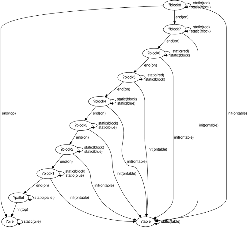
(a) A concrete structure $C$.

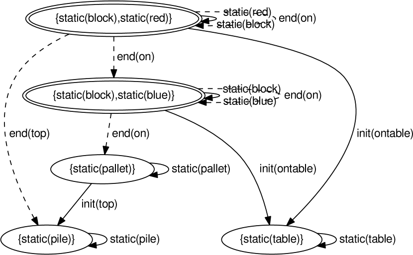
(b) An abstract structure $\mathpzc{S}=\beta(C)$.

Figure 2. Canonical abstraction of the (generalized and abstracted) ‘stack’ experience (in Listing 3) in the stacking-blocks EBPD. Nodes constitute the universe of a structure and edges represent the truth-values of the key-properties over the universe.

The inferred scope is finally represented in a learned activity schema as a set of key-properties. Summary objects are represented as (summary ?c) where ?c is a canonical name. Indefinite values ($\frac{1}{2}$) appear as (maybe($p$)) where $p$ represents a key-property. Listing 6 shows the inferred scope of applicability for the activity schema of the ‘stack’ task.

⬇

(summary {static(block),static(blue)})

(summary {static(block),static(red)})

(static(pile {static(pile)}))

(static(table {static(table)}))

(static(pallet {static(pallet)}))

(static(block {static(block),static(blue)}))

(static(block {static(block),static(red)}))

(static(blue {static(block),static(blue)}))

(static(red {static(block),static(red)}))

(init(top {static(pallet)} {static(pile)}))

(init(ontable {static(block),static(blue)} {static(table)}))

(init(ontable {static(block),static(red)} {static(table)}))

(maybe(end(on {static(block),static(blue)} {static(block),static(blue)})))

(maybe(end(on {static(block),static(blue)} {static(pallet)})))

(maybe(end(on {static(block),static(red)} {static(block),static(red)})))

(maybe(end(on {static(block),static(red)} {static(block),static(blue)})))

(maybe(end(top {static(block),static(red)} {static(pile)})))

Listing 6: The inferred scope of applicability for the learned activity schema of the ‘stack’ task. ‘Summary’ objects represent arbitrary numbers of objects of the same canonical name, and ‘maybe’ key-properties represent key-properties with truth-values of either $0$ or $1$ in a task planning problem.

7. SELECTING AN APPLICABLE ACTIVITY SCHEMA FOR PROBLEM SOLVING

When an activity schema is learned for a class of problems, it can be used to generate a solution plan for a given task problem. In the previous work, the EBPDs framework lacked an automatic strategy to find an applicable activity schema, among several learned activity schemata, for solving a task problem. Here, we extend the previous work in which an activity schema is selected as applicable to solving a given task problem if the task problem is embedded in the scope of the activity schema, i.e., the task problem maps onto the scope of the activity schema. Selecting an activity schema involves problem abstraction and testing the scope of applicability (i.e., embedding).

Given the predicate abstraction hierarchy in $\mathcal{R}$, the abstraction of a problem is achieved by transforming the concrete predicates into abstract predicates, which results in an abstracted task problem. A concrete task problem $\mathcal{P}=(t,\sigma,s_{0},g)$ is translated into an abstracted task problem $\mathcal{P}_{a}=(t,\sigma_{a},{s_{0}}_{a},g_{a})$, denoted by ${\texttt{Abs}}(\mathcal{P})$, as follows:

$$\sigma_{a}=\{{\texttt{parent}}(p)\mid p\in\sigma\},\quad{s_{0}}_{a}=\{{\texttt{parent}}(p)\mid p\in s_{0}\},\quad g_{a}=\{{\texttt{parent}}(p)\mid p\in g\}.$$

To see how the abstracted task problem $\mathcal{P}_{a}$ is embedded in the scope of an activity schema, we first convert $\mathcal{P}_{a}$ into a $2$-valued structure (as described in Section 6), and then test if the obtained $2$-valued structure is embedded in the scope of an activity schema:

Definition 0.

We say that a concrete structure (i.e., an abstracted task problem represented in a $2$-valued logical structure) $C=(U,\iota)$ is embedded in an abstract structure (i.e., in the scope of an activity schema) $\mathpzc{S}=(U^{\prime},\iota^{\prime})$, denoted by $C\sqsubseteq\mathpzc{S}$, if there exists a function $f:U\to U^{\prime}$ such that $f$ is surjective and for every predicate symbol $p^{(k)}$ of arity $k$ with a temporal symbol $\tau$, and tuple of objects $u_{1},...,u_{k}\in U$, one of the following conditions holds:

(1) $$\begin{array}[]{c}\iota(\tau(p))(u_{1},...,u_{k})=\iota^{\prime}(\tau(p))(f(u_{1}),...,f(u_{k}))\quad\text{or}\quad\iota^{\prime}(\tau(p))(f(u_{1}),...,f(u_{k}))=\frac{1}{2}\enspace.\end{array}$$

Further, $\mathpzc{S}$ represents the set of concrete structures embedded in it: $\{C\mid C\sqsubseteq\mathpzc{S}\}$.

Proposition 0.

Canonical abstraction is sound with respect to the embedding relation. That is, $C\sqsubseteq\beta(C)$ holds for every concrete structure $C$.

Proposition 0.

If an abstract structure $\mathpzc{S}=(U^{\prime},\iota^{\prime})$ is in the image of canonical abstraction, then checking whether a concrete structure $C=(U,\iota)$ is embedded in $\mathpzc{S}$ can be done in time polynomial in $|U|+|U^{\prime}|+|K|$.

Proof sketch. Observe that (1) implies, if $C$ is embedded in $\mathpzc{S}$, then $\mathpzc{S}$ and $C$ have equal sets of canonical names (checkable in polynomial time). Therefore, the embedding function must be $f=\{u\mapsto u^{\prime}\mid{\texttt{canon}}_{C}(u)={\texttt{canon}}_{\mathpzc{S}}(u^{\prime})\}$. Checking that (1) holds for $f$ takes polynomial time. ∎

Based on the above definition, we implemented and integrated an Embedding function into the EBPDs system to find an applicable activity schema $m=(h,\mathpzc{S},\Omega)$ to a task planning problem $\mathcal{P}=(t,\sigma,s_{0},g)$, by checking whether $\texttt{Struct}({\texttt{Abs}}(\mathcal{P}))\sqsubseteq\mathpzc{S}$ holds.

8. PLANNING USING THE LEARNED ACTIVITY SCHEMATA

We have previously proposed a planning system for generating a solution plan to a given task problem using a learned activity schema (Mokhtari et al., 2017a, b). Problem solving in EBPDs is achieved using a hierarchical problem solver which includes an abstract planner—Abstract Schema-Based Planner (ASBP), and a concrete planner—Schema-Based Planner (SBP). Given an experience-based planning domain $\Delta=(\mathcal{D}_{a},\mathcal{D}_{c},\mathcal{R},\mathcal{E},\mathcal{M})$ and a task planning problem $\mathcal{P}$, the EBPDs’ planning system retrieves an applicable activity schema $m=(t,\mathpzc{S},\Omega)$, i.e., checks $\texttt{Struct}({\texttt{Abs}}(\mathcal{P}))\sqsubseteq\mathpzc{S}$ (see Section 7), and attempts to generate a solution plan to $\mathcal{P}$.

Using the abstract planning domain $\mathcal{D}_{a}$, ASBP first derives an abstract solution by instantiating the enriched abstract plan $\Omega$ for ${\texttt{Abs}}(\mathcal{P})$. This also involves extending possible loops in $\Omega$ for the applicable objects in ${\texttt{Abs}}(\mathcal{P})$. To extend a loop, ASBP simultaneously generates all successors for an iteration of the loop and for the following enriched abstract operator after the loop. ASBP computes a cost for all generated successors based on the number of features of abstract operators verified with the features extracted for the instantiated abstract actions, and selects the best current action with the lowest cost during the search. Finally, a ground abstract plan, $\Pi$, is generated when ASBP gets the end of (the enriched abstract plan) $\Omega$ (where the goal must also be achieved).

The ground abstract plan $\Pi$ produced by ASBP becomes the main skeleton of the final solution based on which SBP, using the concrete planning domain $\mathcal{D}_{c}$, produces a final solution plan to $\mathcal{P}$ by generating and substituting concrete actions for the abstract actions in $\Pi$ (as specified in the operator abstraction hierarchy in $\mathcal{R}$). This might also involve generating and inserting actions from the $\varnothing$ ($nil$) class (see Table 2).

The specific planning algorithm and its respective implementation have been proposed and described in (Mokhtari et al., 2017a, b).

9. EMPIRICAL EVALUATION

We present the results of our experiments in different classes of problems.

9.1. Prototyping and implementation

We implemented a prototype of our system in SWI-Prolog, which is a general-purpose logic programming language for fast prototyping artificial intelligence techniques, and used TVLA as an engine for computing the scope of applicability of activity schemata. We performed all experiments in simulated domains and simulated robot platforms, e.g., PR2, on a machine $2.20$GHz Intel Core i$7$ with $12$G memory.

9.2. STACKING-BLOCKS

In our first experiment, we use the stacking-blocks EBPD, as described in Section 3 (see also Tables 1 and  2). The main objective of this experiment is to learn a set of different activity schemata (tasks) with the same goal but different scopes of applicability, and to evaluate how the scope testing (embedding) function allows the system to automatically find an applicable activity schema to a given task problem. In this paper, we described a class of ‘stack’ problems (Section 3) with an experience (Listing 2), a learned activity schema (Listing 5), and its scope of applicability (Listing 6 and Figure 2(b)).

Additionally, we define three other classes of the ‘stack’ problems with the same goal but different initial configurations as follow: (i) a pile of red and blue blocks, with red blocks at the bottom and blue blocks on top; (ii) a pile of alternating red and blue blocks, with a blue block at the bottom and a red block on top; and (iii) a pile of alternating red and blue blocks, with a red block at the bottom and a blue block on top. In all classes of problems, the goal is to make a new pile of red and blue blocks with blue blocks at the bottom and red blocks on top (the same goal as in Section 3).

To show the effectiveness of the proposed scope of applicability inference, we simulated an experience (containing an equal number of $20$ blocks of red and blue colors) in each of above classes, which based on them the system generates three activity schemata with distinct scopes of applicability (see Figure 3).

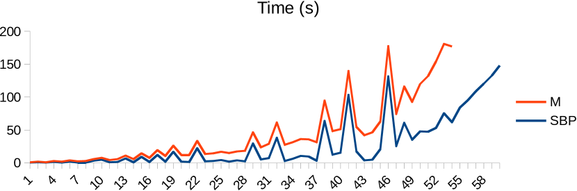
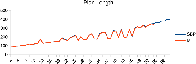
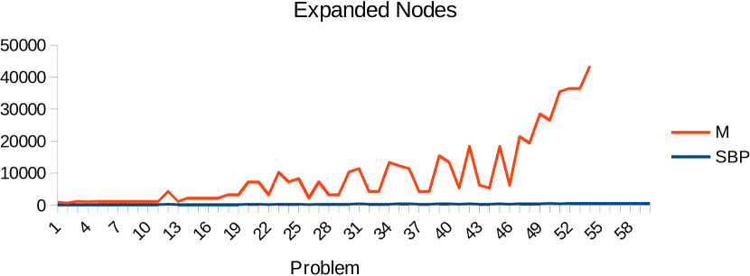
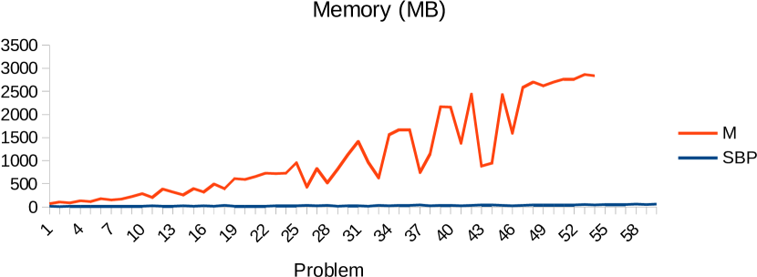
Figure 5. Performance of the SBP and Madagascar (M) in the stacking-blocks domain.

To evaluate the system over the learned activity schemata, we randomly generated $60$ task problems in all four classes of the ‘stack’ tasks ($15$ in each class), ranging from $20$ to $50$ equal number of red and blue blocks in each problem. In this experiment, the system found an applicable activity schema (among $4$) to solve given task problems in under $60\text{ms}$ for testing the scope of applicability (see Figure 4), and then successfully solved all problems. To show the efficiency of the system, we also evaluated and compared the performance of the SBP with a state-of-the-art planner, Madagascar (Rintanen, 2012), based on four measures: time, memory, number of evaluated nodes and plan length (see Table 3). In this experiment, SBP was extremely efficient in terms of memory and evaluated nodes in the search tree. SBP was also fairly fast to solve some problems comparing to Madagascar. Note that the time comparison is not accurate in this evaluation, since SBP has been implemented in Prolog, but, by contrast, Madagascar has been implemented in C++. Figure 5 alternatively summarizes the performance of the two planners.

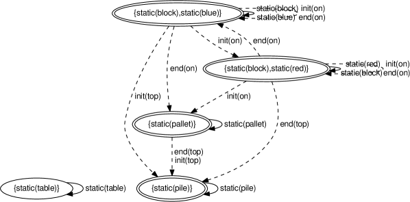
(a) This scope of applicability (abstract structure) represents all ‘stack’ problems that have exactly one table and at least one pile, one pallet, one blue block and one red block such that blue blocks are initially on top of red blocks and finally red blocks are on top of blue blocks (on a pallet) on a pile.

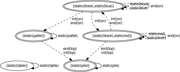
(b) This scope of applicability represents all ‘stack’ problems that have exactly one table and at least one pile, one pallet, one blue block and one red block such that alternate red and blue blocks are initially on a pile with a blue block at the bottom (on a pallet) and a red block on top and finally red blocks are on top of blue blocks.

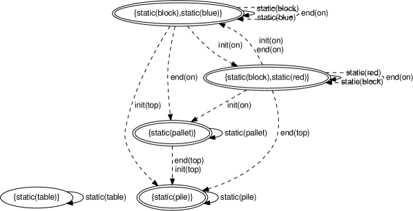
(c) This scope of applicability represents all ‘stack’ problems that have exactly one table and at least one pile, one pallet, one blue block and one red block such that alternate red and blue blocks are initially on a pile with a red block at the bottom (on a pallet) and a blue block on top and finally red blocks are on top of blue blocks.

Figure 3. The scope of applicability, i.e., canonical abstraction, of the additional three classes of the ‘stack’ task in the stacking-blocks EBPD.

Table 3. Performance of the SBP and Madagascar (M) planners in terms of applicability test (retrieval) time, search time, memory, developed nodes and plan length in the different classes of ‘stack’ problems in the stacking-blocks EBPD.

Problem/	Retrieval∗ time (s)	Search time (s)		Memory (MB)		Evaluated states		Plan length
(#blocks)	SBP	SBP	M	SBP	M	SBP	M	SBP	M
p1    (22)	0.011	0.29	0.550	10.6	57.2	131	813	87	87
p2    (22)	0.022	0.90	0.820	8.1	92.5	133	597	88	88
p3    (24)	0.010	0.37	0.820	12.4	76.9	143	1011	95	95
p4    (24)	0.021	1.44	1.250	8.9	124.9	145	985	96	96
p5    (26)	0.010	0.49	1.290	13.9	100.2	155	1k	103	103
p6    (26)	0.023	2.16	1.780	9.8	162.4	157	1k	104	104
p7    (28)	0.010	0.61	1.780	15.9	130.2	167	1k	111	111
p8    (30)	0.010	0.77	2.360	17.3	148.8	179	1k	119	119
p9    (28)	0.026	3.22	2.750	10.3	212.9	169	1k	112	112
p10  (30)	0.029	4.67	3.170	11.4	271.2	181	1k	120	127
p11  (32)	0.010	0.95	3.330	19.7	187.10	191	1k	127	127
p12  (22)	0.035	1.48	4.220	16.9	369.7	271	4k	172	172
p13  (32)	0.023	6.84	4.460	12.5	307.4	193	1k	128	128
p14  (34)	0.010	1.16	4.570	22.1	238.5	203	2k	135	135
p15  (34)	0.022	9.14	5.270	13.5	382.8	205	2k	136	136
p16  (36)	0.010	1.43	6.390	24.1	296.7	215	2k	143	143
p17  (36)	0.026	12.31	6.900	13.9	478.5	217	2k	144	144
p18  (38)	0.014	1.73	8.770	26.9	366.7	227	3k	151	151
p19  (38)	0.028	16.87	9.200	15.0	592.2	229	3k	152	152
p20  (24)	0.055	2.05	9.950	17.7	577.7	288	7k	191	184
p21  (22)	0.048	1.33	10.930	16.1	642.6	264	7k	175	168
p22  (40)	0.024	22.23	11.100	16.1	714.4	241	3k	160	160
p23  (24)	0.032	2.30	11.190	19.4	698.8	296	10k	188	188
p24  (26)	0.046	3.04	11.630	20.1	709.5	312	7k	207	200
p25  (28)	0.050	4.50	12.560	22.5	929.2	336	8k	223	216
p26  (40)	0.010	2.07	12.900	29.7	401.1	239	2k	159	159
p27  (26)	0.039	3.78	13.530	21.9	802.6	321	7k	204	204
p28  (42)	0.011	2.48	16.120	31.5	491.7	251	3k	167	167
p29  (42)	0.023	29.52	16.930	17.3	799.7	253	3k	168	168
p30  (28)	0.040	5.27	18.330	23.7	1098.0	346	10k	220	220
p31  (30)	0.037	7.50	21.680	26.6	1388.7	371	11k	236	236
p32  (44)	0.022	38.26	23.090	17.9	947.1	265	4k	176	176
p33  (44)	0.014	2.96	24.690	35.0	593.8	263	4k	175	175
p34  (30)	0.046	6.50	24.980	24.1	1537.7	360	13k	239	232
p35  (32)	0.039	10.69	25.570	28.5	1645.8	396	12k	252	252
p36  (32)	0.046	9.71	26.170	26.8	1645.7	384	11k	255	248
p37  (46)	0.010	3.48	27.970	38.4	709.6	275	4k	183	183
p38  (46)	0.022	63.59	31.420	19.1	1128.5	277	4k	184	184
p39  (34)	0.058	12.68	35.910	29.5	2140.1	408	15k	271	264
p40  (34)	0.040	15.41	36.030	31.7	2126.8	421	13k	268	268
p41  (48)	0.022	103.44	36.120	20.3	1359.2	289	5k	192	192
p42  (36)	0.054	17.65	37.100	31.5	2410.5	432	18k	287	280
p43  (48)	0.010	4.06	37.820	41.9	841.0	287	6k	191	191
p44  (50)	0.014	4.72	41.650	44.7	904.3	299	5k	199	199
p45  (36)	0.040	20.64	42.470	34.9	2397.2	446	18k	284	284
p46  (50)	0.022	131.65	45.770	21.6	1575.5	301	6k	200	207
p47  (38)	0.048	25.80	48.710	34.5	2553.2	456	21k	303	296
p48  (40)	0.034	60.81	55.480	40.0	2658.5	496	19k	316	316
p49  (38)	0.042	35.48	57.540	38.1	2586.7	471	28k	300	300
p50  (42)	0.053	47.82	72.320	40.6	2665.7	504	26k	335	328
p51  (40)	0.061	47.58	84.570	37.5	2727.0	480	35k	319	312
p52  (42)	0.039	53.22	101.080	43.7	2724.10	521	36k	332	332
p53  (44)	0.037	75.32	105.530	47.4	2817.1	546	36k	348	348
p54  (44)	0.049	62.14	114.780	42.6	2793.1	528	43k	351	344
p55  (46)	0.048	84.28	–	46.0	–	552	–	367	–
p56  (46)	0.034	95.31	–	51.1	–	571	–	364	–
p57  (48)	0.056	108.66	–	49.5	–	576	–	383	–
p58  (48)	0.038	120.24	–	53.8	–	596	–	380	–
p59  (50)	0.050	132.46	–	51.6	–	600	–	399	–
p60  (50)	0.040	147.93	–	57.9	–	621	–	396	–

^∗ An average time of retrieving an activity schema (i.e., in this experiment among four learned activity schemata) for each task problem. The retrieval time increases linearly with the number of learned activity schemata for a specific task.

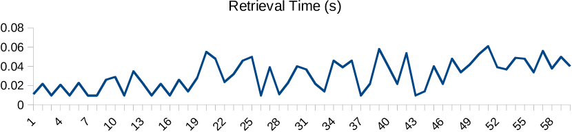
Figure 4. CPU time used by SBP to find an applicable activity schema (among 4) for solving problems in the stacking-blocks domain.

9.3. ROVER

In the second experiment, we used the rover domain from the 3rd International Planning Competition (IPC-3). In this experiment, we adopt a different approach for evaluating the proposed scope inference technique. We randomly generated $50$ problems containing exactly $1$ rover and ranging from $1$ to $3$ waypoints, $5$ to $30$ objectives, $5$ to $10$ cameras and $5$ to $20$ goals in each problem. Using the scope inference procedure, the problems are classified into $9$ sets of problems. That is, problems that converge to the same $3$-valued structure are put together in the same set. Hence, each set of problems is identified with a distinct scope of applicability. Figure 6(a) shows the time required to classify the problems into different sets, i.e., the time required by TVLA to generate $3$-valued structures for the problems and test which problems converge to the same $3$-valued structure. Figure 6(b) shows the distribution of the problems in the obtained sets of problems. In each set of problems, we simulated an experience and generated an activity schema for problem solving. Figure 7 shows the time required to retrieve an applicable activity schema (among 9 activity schemata in this experiment) for solving given problems, i.e., the time required to check whether a given problem is embedded in the scope of an activity schema. SBP successfully solved all problems in each class.

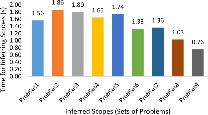
(a)

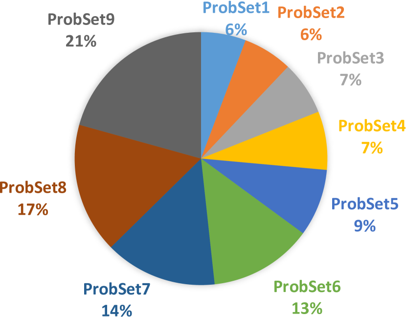
(b)

Figure 6. CPU time used by TVLA to classify the problems (a), and distribution of the problems in the obtained problem sets (b) in the rover domain

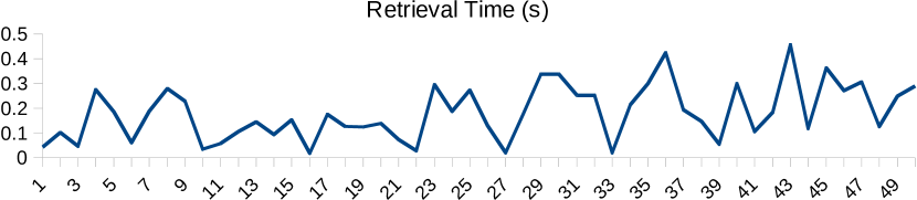
Figure 7. CPU time used by SBP to find an applicable activity schema (among 9) for solving problems in the rover domain.

9.4. CAFE

In order to validate the practical utility of our approach, we also applied it to a real-world task using a fully physically simulated PR2 in Gazebo, the standard simulator in ROS. We developed a cafe EBPD including $14$ concrete and $4$ abstract planning operators (see Table 4). We use a coffee serving demonstration including two Scenarios A and B with different sets of instructions to teach a PR2 to serve a guest in a cafe environment (see Figure 8). Instructions for Scenario A is “Move to counter1, grasp mug1, move to south of table1, place mug1 at the right placement area of guest1 – this is a ServeACoffee task.” Instructions for Scenario B is “Move to counter1, grasp mug1 and mug2, move to south of table1, place mug1 at the right placement area of guest1, move to north of table1, place mug2 at the left placement area of guest1 – this is also a ServeACoffee task.” In both scenarios, it is assumed that the robot knows the location of the guest and of the placement areas on the table. However, it does not know which placement area to approach for a guest. We used the infrastructure and simulation environment of the RACE project (Hertzberg et al., 2014) for instruction-based teaching of the robot to achieve the tasks. Figure 9 shows the snapshots of teaching the PR2 a ServeACoffee task in Scenario A in Gazebo.

Table 4. Abstract and planning operators in the cafe EBPD.

Abstract operators	Concrete operators
move/3	move-base/3
move/3	move-base-blind/3
pick/4	pick-up-object/8
place/4	place-object/8
$\varnothing$	tuck-arm/5
$\varnothing$	move-arm-to-carry/5
$\varnothing$	move-arm-to-side/5
$\varnothing$	move-torso-down/5
$\varnothing$	move-torso-middle/5
$\varnothing$	move-torso-up/5
$\varnothing$	ready-to-safe-move-with-no-object/8
$\varnothing$	ready-to-safe-move-with-one-object/9
$\varnothing$	ready-to-safe-move-with-two-object/10
$\varnothing$	observe-object-on-area/4

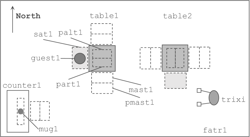
(a) Scenario A

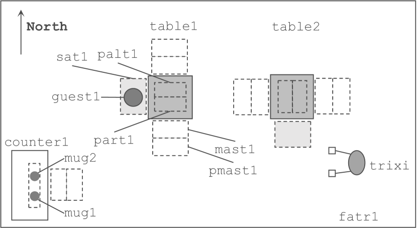
(b) Scenario B

Figure 8. Initial states of the restaurant floor for the ServeACoffee demonstration in Scenarios A and B with a PR2. (a) In Scenario A, PR2 is taught to take mug1 from counter1 and approaches the south of table1 and place mug1 on the right side of guest1. (b) In Scenario B, PR2 is taught to take mug1 and mug2 from counter1 and approaches the south of table1 and place mug1 on the right side of guest1, and then approaches the north of table1 and place mug2 on the left side of guest1.

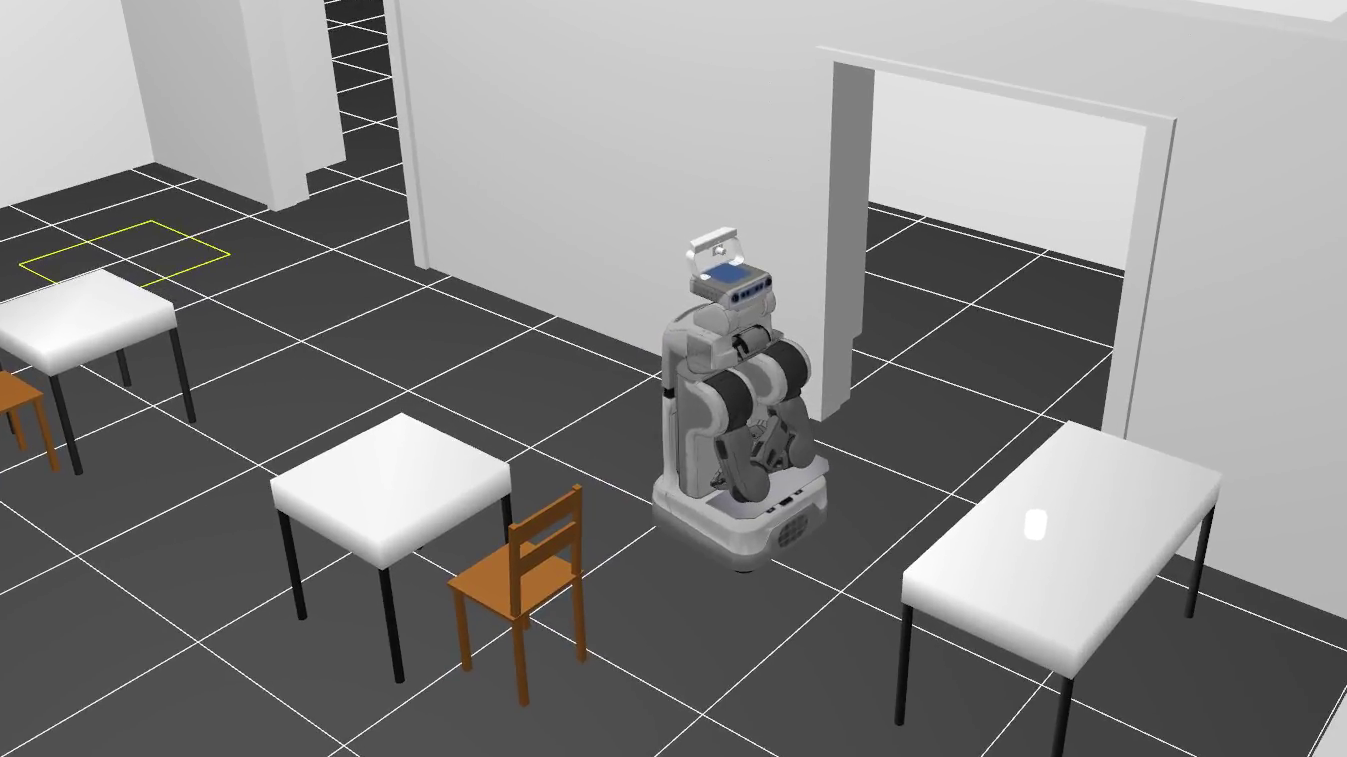
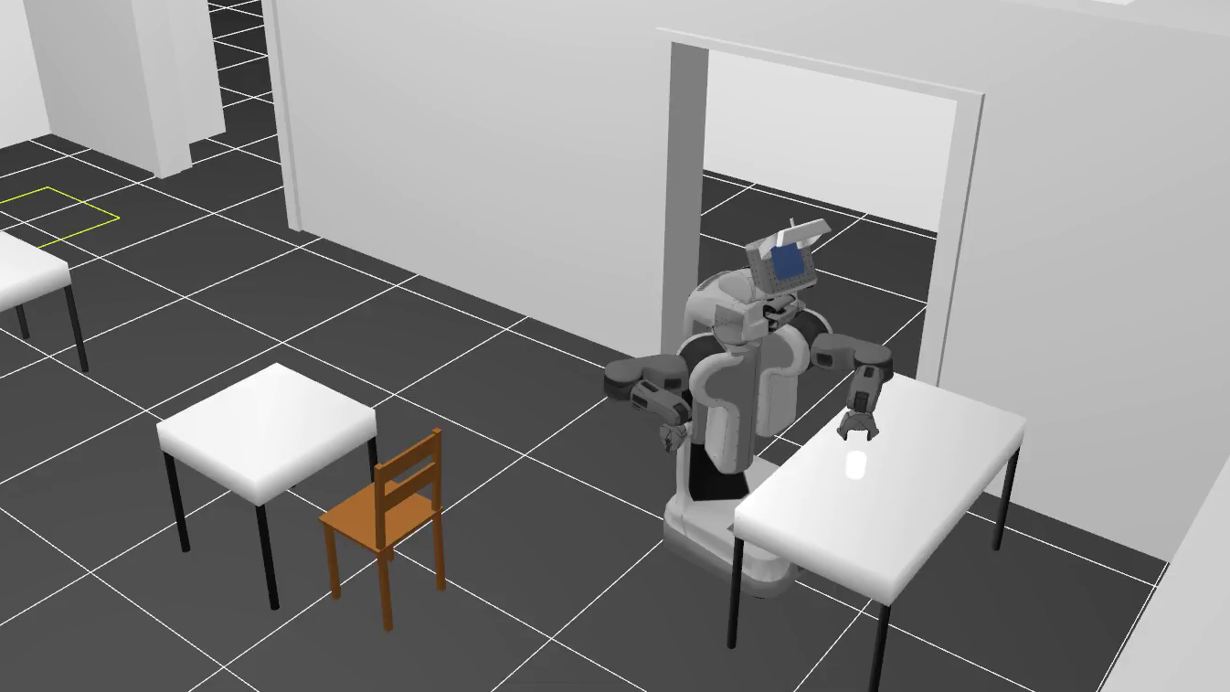
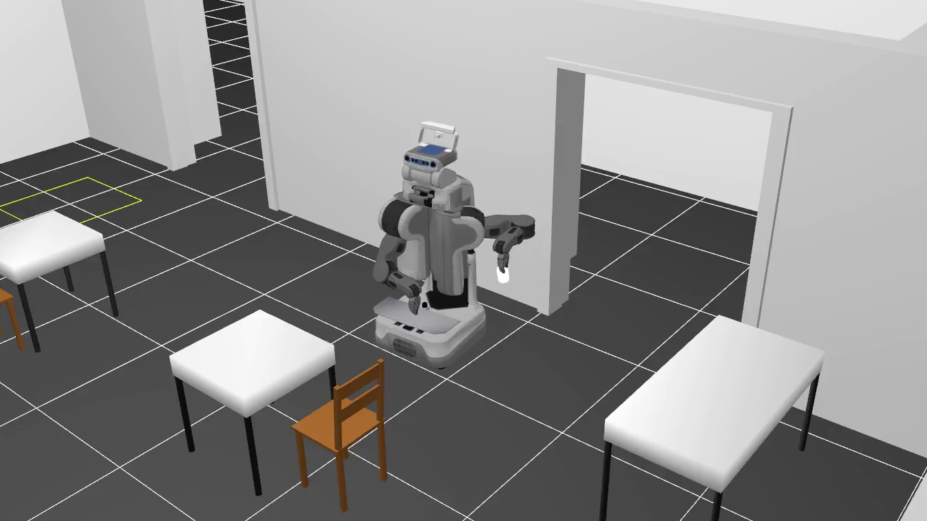
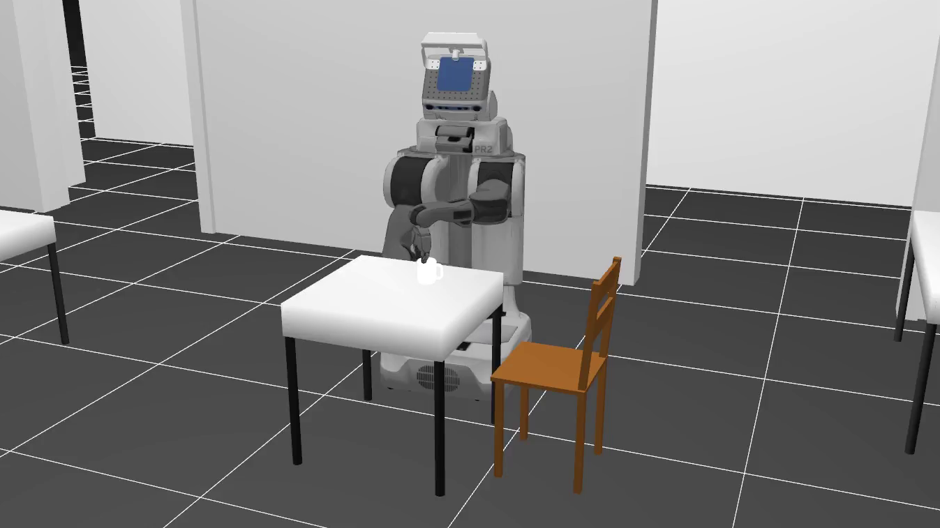
Figure 9. An example of the execution of a ServeACoffee task with a PR2 in Gazebo simulated environment. In this scenario, (from left to right) robot moves to a counter, picks up a mug from the counter, moves to a table, and puts the mug on the table in front of a guest.

Our system learned two activity schemata for ServeACoffee task with distinct abstract plans (i.e, different instructions sets) and distinct scopes of applicability. To validate the utility of the learned activity schemata, we setup two test scenarios in each class of ServeACoffee task in which the robot is asked for serving a guest sitting at table2. Our system computes the solution plans for each task problem using the learned activity schemata in less than $1$ second. Video of the PR2 doing ServeACoffee tasks in this experiment are available at https://goo.gl/HJ6g2R and https://github.com/mokhtarivahid/ebpd/tree/master/demos.

The domains, experiences, learned activity schemata and given task problems used in our experiments are available online by the link: https://github.com/mokhtarivahid/ebpd/.

10. CONCLUSION AND FUTURE WORK

We proposed an approach to generate a set of conditions that determines the scope of applicability of an activity schema in experience-based planning domains (EBPDs). The inferred scope allows an EBPD system to automatically find an applicable activity schema for solving a task problem, among several learned activity schemata for a specific task.

We validated the utility of this work in a simulated domain and a fully physically simulated PR2 in Gazebo. Through our experiments, we demonstrated the effectiveness of the system, including loop detection and scope inference procedures. We showed the timing results for test problems in these experiments. The time required for learning activity schemata, and computing and testing their scopes were negligible. The system learned activity schemata from single examples in under seconds, in contrast to other machine learning techniques, addressed in the related work, which usually require large sets of plan traces to learn planning domain knowledge (e.g., HTN-Maker (Hogg et al., 2008) uses 75 out of 100 input problems to train the system).

While the results show good scalability, many engineering optimizations are possible on our prototype implementation of the proposed algorithms. Faster results can be obtained from an implementation in a compiled language. Extensive evaluation of the proposed system on a large set of domains is also part of the future work.

- (1)
- Allen et al. (2007) James Allen, Nathanael Chambers, George Ferguson, Lucian Galescu, Hyuckchul Jung, Mary Swift, and William Taysom. 2007. PLOW: A collaborative task learning agent. In AAAI, Vol. 7. 1514–1519.
- Argall et al. (2009) Brenna D. Argall, Sonia Chernova, Manuela Veloso, and Brett Browning. 2009. A survey of robot learning from demonstration. Robotics and Autonomous Systems 57, 5 (2009), 469 – 483.
- Billard et al. (2008) Aude Billard, Sylvain Calinon, Ruediger Dillmann, and Stefan Schaal. 2008. Robot programming by demonstration. In Springer handbook of robotics. Springer, 1371–1394.
- Borrajo et al. (2015) Daniel Borrajo, Anna Roubíčková, and Ivan Serina. 2015. Progress in case-based planning. ACM Computing Surveys (CSUR) 47, 2, Article 35 (Jan 2015), 39 pages.
- Bylander (1994) Tom Bylander. 1994. The computational complexity of propositional STRIPS planning. Artificial Intelligence 69, 1-2 (1994), 165–204.
- Chao et al. (2011) Crystal Chao, Maya Cakmak, and Andrea L Thomaz. 2011. Towards grounding concepts for transfer in goal learning from demonstration. In Development and Learning (ICDL), 2011 IEEE International Conference on, Vol. 2. IEEE, 1–6.
- Chrpa (2010) Lukáš Chrpa. 2010. Generation of macro-operators via investigation of action dependencies in plans. The Knowledge Engineering Review 25, 03 (2010), 281–297.
- Fawcett and Utgoff (1992) Tom E Fawcett and Paul E Utgoff. 1992. Automatic feature generation for problem solving systems. In Machine Learning Proceedings 1992. Elsevier, 144–153.
- Fikes et al. (1972) Richard E Fikes, Peter E. Hart, and Nils J Nilsson. 1972. Learning and executing generalized robot plans. Artificial intelligence 3 (1972), 251–288.
- Ghallab et al. (2004) Malik Ghallab, Dana Nau, and Paolo Traverso. 2004. Automated planning: theory & practice. Elsevier.
- Hammond (1986) Kristian J Hammond. 1986. CHEF: a model of case-based planning. In Proceedings of the Fifth National Conference on Artificial Intelligence. AAAI Press, 267–271.
- Hertzberg et al. (2014) Joachim Hertzberg, Jianwei Zhang, Liwei Zhang, Sebastian Rockel, Bernd Neumann, Jos Lehmann, KrishnaS.R. Dubba, AnthonyG. Cohn, Alessandro Saffiotti, Federico Pecora, Masoumeh Mansouri, Štefan Konec̆ný, Martin Günther, Sebastian Stock, Luís Seabra Lopes, Miguel Oliveira, GiHyun Lim, Hamidreza Kasaei, Vahid Mokhtari, Lothar Hotz, and Wilfried Bohlken. 2014. The RACE project. KI - Künstliche Intelligenz 28, 4 (2014), 297–304.
- Hogg et al. (2008) Chad Hogg, Héctor Munoz-Avila, and Ugur Kuter. 2008. HTN-MAKER: learning HTNs with minimal additional knowledge engineering required. In Proceedings of the Twenty-Third AAAI Conference on Artificial Intelligence. AAAI Press, 950–956.
- Ilghami and Nau (2006) Okhtay Ilghami and Dana S Nau. 2006. Learning to do HTN planning. In 16st International Conference on Automated Planning and Scheduling (ICAPS). AAAI Press, 390–393.
- Ilghami et al. (2002) Okhtay Ilghami, Dana S Nau, Héctor Munoz-Avila, and David W Aha. 2002. CaMeL: learning method preconditions for HTN planning. In Proceedings of the Sixth International Conference on Artificial Intelligence Planning Systems (AIPS). 131–142.
- Ilghami et al. (2005) Okhtay Ilghami, Dana S Nau, Héctor Munoz-Avila, and David W Aha. 2005. Learning preconditions for planning from plan traces and HTN structure. Computational Intelligence 21, 4 (2005), 388–413.
- Kleene (1952) Stephen Cole Kleene. 1952. Introduction to metamathematics. Vol. 483. D. Van Nostrand Co., Inc., New York, N. Y.
- Lev-Ami and Sagiv (2000) Tal Lev-Ami and M Sagiv. 2000. TVLA: A framework for kleene logic based static analyses. Master’s thesis, Tel Aviv University (2000).
- Lev-Ami and Sagiv (2000) Tal Lev-Ami and Shmuel Sagiv. 2000. TVLA: A system for implementing static analyses. In Static Analysis, 7th International Symposium, SAS 2000, Santa Barbara, CA, USA, June 29 - July 1, 2000, Proceedings. 280–301.
- Manber and Myers (1993) Udi Manber and Gene Myers. 1993. Suffix arrays: a new method for on-line string searches. SIAM J. Comput. 22, 5 (1993), 935–948.
- Mitchell et al. (1986) Tom M. Mitchell, Richard M. Keller, and Smadar T. Kedar-Cabelli. 1986. Explanation-based generalization: a unifying view. Machine Learning 1, 1 (1986), 47–80.
- Mokhtari et al. (2016a) Vahid Mokhtari, GiHyun Lim, Luís Seabra Lopes, and Armando J. Pinho. 2016a. Gathering and conceptualizing plan-based robot activity experiences. In Intelligent Autonomous Systems 13, Emanuele Menegatti, Nathan Michael, Karsten Berns, and Hiroaki Yamaguchi (Eds.). Advances in Intelligent Systems and Computing, Vol. 302. Springer International Publishing, 993–1005.
- Mokhtari et al. (2016b) Vahid Mokhtari, Luís Seabra Lopes, and Armando J. Pinho. 2016b. Experience-based planning domains: an integrated learning and deliberation approach for intelligent robots. Journal of Intelligent & Robotic Systems 83, 3 (2016), 463–483.
- Mokhtari et al. (2016c) Vahid Mokhtari, Luís Seabra Lopes, and Armando J. Pinho. 2016c. Experience-based robot task learning and planning with goal inference. In 26st International Conference on Automated Planning and Scheduling (ICAPS). AAAI Press, 509–517.
- Mokhtari et al. (2017a) Vahid Mokhtari, Luís Seabra Lopes, and Armando J. Pinho. 2017a. An approach to robot task learning and planning with loops. In 2017 IEEE/RSJ International Conference on Intelligent Robots and Systems (IROS). 6033–6038.
- Mokhtari et al. (2017b) Vahid Mokhtari, Luís Seabra Lopes, and Armando J. Pinho. 2017b. Learning robot tasks with loops from experiences to enhance robot adaptability. Pattern Recognition Letters 99, Supplement C (2017), 57 – 66. https://doi.org/10.1016/j.patrec.2017.06.003 User Profiling and Behavior Adaptation for Human-Robot Interaction.
- Rintanen (2012) Jussi Rintanen. 2012. Planning as satisfiability: heuristics. Artificial Intelligence 193 (2012), 45 – 86.
- Sagiv et al. (2002) Shmuel Sagiv, Thomas W. Reps, and Reinhard Wilhelm. 2002. Parametric shape analysis via 3-valued logic. ACM Trans. Program. Lang. Syst. 24, 3 (2002), 217–298.
- Srivastava et al. (2011) Siddharth Srivastava, Neil Immerman, and Shlomo Zilberstein. 2011. A new representation and associated algorithms for generalized planning. Artificial Intelligence 175, 2 (2011), 615 – 647.
- Winner and Veloso (2007) Elly Winner and Manuela M. Veloso. 2007. LoopDISTILL: learning domain-specific planners from example plans. In Workshop on AI Planning and Learning, ICAPS.