Quantum signatures of chaos, thermalization and tunneling in the exactly solvable few body kicked top

Abstract

Exactly solvable models that exhibit quantum signatures of classical chaos are both rare as well as important - more so in view of the fact that the mechanisms for ergodic behavior and thermalization in isolated quantum systems and its connections to non-integrability are under active investigation. In this work, we study quantum systems of few qubits collectively modeled as a kicked top, a textbook example of quantum chaos. In particular, we show that the 3 and 4 qubit cases are exactly solvable and yet, interestingly, can display signatures of ergodicity and thermalization. Deriving analytical expressions for entanglement entropy and concurrence, we see agreement in certain parameter regimes between long-time average values and ensemble averages of random states with permutation symmetry. Comparing with results using the data of a recent transmons based experiment realizing the 3-qubit case, we find agreement for short times, including a peculiar step-like behaviour in correlations of some states. In the case of 4-qubits we point to a precursor of dynamical tunneling between what in the classical limit would be two stable islands. Numerical results for larger number of qubits show the emergence of the classical limit including signatures of a bifurcation.

I Introduction

In a modest pursuit of the esthetic attributed to the probabilist Feller that “the best consists of the general embodied in the concrete” Billingsley , we consider extreme quantum cases of the kicked top, a widely studied text-book model of quantum chaos Haake ; Peres02 ; KusScharfHaake1987 ; KusMostowskiHaake1988 ; Zyczkowski1990 ; Gerwinski1995 ; Wang2004 ; LombardiMatzkin2011 ; Ghose ; mrgi14 ; Lewenstein-arxiv-2018 ; Bhosale-pre-2017 , which has also been implemented in experiments Chaudhary ; Neill16 . The general issues at hand are the emergence of classical chaos from a linear quantum substratum and, more recently, the role of quantum chaos in the thermodynamics of closed quantum systems CassidyEtal2009 ; SantosRigol2010 ; Rigol16 . Vigorous progress is being made in studying thermalization of isolated quantum systems that could be either time-independent or periodically forced JensenShankar1985 ; Deutsch91 ; Srednicki94 ; Rigol2009 ; CassidyEtal2009 ; SantosRigol2010 ; CiracHastings2011 ; DeutchLiSharma2013 ; LangenEtal2013 ; Rigol16 ; LucaRigol2014 ; LazaDasMoess2014 ; LazDasMoess2014pre ; Haldar2018 ; Neill16 ; Kaufman2016 ; ClosEtal2016 ; HazzardEtal2014 . Entanglement within many-body states in such quantum chaotic systems drives subsystems to thermalization although the full state remains pure and of zero entropy, see Kaufman2016 for a demonstration with cold atoms.

Quantum chaos Gutzwiller1990 ; Haake and, consequently, eigenstate thermalization hypothesis Srednicki94 ; Rigol16 enables one to use individual states for ensemble averages. For periodically driven systems that do not even conserve energy, a structureless “infinite-temperature” ensemble emerges in strongly non-integrable regimes LucaRigol2014 ; LazDasMoess2014pre . A recent 3-qubit experiment, using superconducting Josephson junctions, that simulated the kicked top Neill16 (see also Madhok2018_corr ) purported to remarkably demonstrate such a thermalization. Although such behavior has been attributed to non-integrability Neill16 ; Rigol16 , we exactly solve this 3-qubit kicked top and also point out that it can be interpreted as a special case of an integrable model, the well-known transverse field Ising model. Interestingly, we also solve the 4-qubit case exactly, where there is no such evident connection to an already known integrable model.

The Arnold-Liouville notion of integrability requires sufficient number of independent constants of motion in involution. It is well-known that in finite dimensional quantum systems this notion can be debated, wherein any system is integrable as the projectors on eigenstates form a set of independent mutually commuting quantities, for example see YusShastry2013 . However, in this work, we use integrability more in the sense of the traditional definition of the existence of constants that arise from symmetries and whose forms are independent of the parameters of the system. This is a pragmatic approach and in line with current understanding that would classify the nearest neighbor transverse field Ising model as integrable and one with an additional longitudinal field, or a transverse field Ising model with nearest as well as next-nearest neighbor interactions as non-integrable.

Nonintegrable, chaotic, systems may be solvable in some tangible sense, the textbook examples of the tent map and the bakers map are solvable, despite being completely chaotic. The Arnold cat map, and its quantizations also admit analytical solutions despite being hyperbolic and chaotic. Nevertheless, this is very rare, and restricted to abstract models. No known model that has a mixed phase space, with both regular and chaotic orbits, is also known to be exactly solvable in the same sense. Attempts at constructing such models include the piecewise linear “lazy bakers map”. The kicked top, in the limit of an infinite number of qubits displays a standard transition to Hamiltonian chaos, including a mixed phase space, and it is remarkable that many of the features are already reflected in the solvable few qubit cases as we show in this paper.

For example, we obtain explicit formulas for entanglements generated for the 3 and 4-qubit cases and the compare the former with data from the experiment in Neill16 and find very good agreement. The infinite time average of single qubit entanglement is found analytically for some initial states and at a special and large value of the forcing, for all initially unentangled coherent states. These are shown to tend to that obtained from relevant (random matrix) ensembles, in some cases even exactly coinciding with them and thus displaying thermalization. These demonstrate that even in the deep quantum regime, the transition to what in the classical limit becomes chaos is reflected in the time-averaged entanglement. While the connections between chaos and entanglement in the semiclassical regime is now well studied MillerSarkar ; Wang2004 ; LombardiMatzkin2011 ; Ghose ; trail2008entanglement ; Lewenstein-arxiv-2018 ; Lakshminarayan ; BandyopadhyayArul2002 ; Bandyopadhyay04 ; ScottCaves2003 ; Ghose ; Lakshminarayan16 , such systems are typically not analytically tractable and appeal is made to statistical modeling based on random matrix theory. Remarkably, there are interesting quantum effects in the few-body systems we study here. We find the presence of dynamical tunneling DavisHeller1981 ; LinBallentine1990 ; Peres1991 ; Tomsovic98b ; SrihariBook between what appears in the classical limit as symmetric regular regions. This results in extremely slow convergence of subsystem entropies in the near-integrable regime that happens for some states of the 4-qubit case. In the near-integrable regime the exactly calculable tunneling splitting is shown to result in this long-time dynamics. The kicked-top experiment involving the spin of cold Cs atoms has already observed such tunneling Chaudhary but our observations provide a connection between the number of qubits and a system parameter at which such tunneling occurs. This may open windows to study the interplay of chaos and tunneling even in systems having a small number of qubits.

I.1 The model

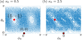
Figure 1: (a) Regular and (b) mixed phase space structures resulting from the classical chaotic dynamics. Points labelled with red square and red circle correspond to initial states $\Theta=0,\Phi=0$ on a period-4 orbit and $\Theta=\pi/2,\Phi=-\pi/2$ at the centre of regular island respectively.

The quantum kicked top is a combination of a rotation and a torsion, the Hamiltonian KusScharfHaake1987 ; Haake ; Peres02 is given by

$$H=\frac{\kappa_{0}}{2j}{J_{z}}^{2}\sum_{n=-\infty}^{\infty}\delta(t-n\tau)+\frac{p}{\tau}\,{J_{y}}.$$ (1)

Here $J_{x,y,z}$ are components of the angular momentum operator $\mathbf{J}$. The time between periodic kicks is $\tau$. The Floquet map is the unitary operator,

$$\mathcal{U}=\exp\left[-i(\kappa_{0}/2j\hbar)J_{z}^{2}\right]\exp\left[-i(p/\hbar)J_{y}\right],$$ (2)

which evolves states just after a kick to just after the next. The parameter $p$ measures rotation about the $y$ axis, and in the following we set $\hbar=1$ and $p=\pi/2$. The parameter $\kappa_{0}$, which is the magnitude of a twist applied between kicks controls the transition and measure of chaos. If it vanishes, the dynamics is simply a rotation. As the magnitude of the total angular momentum is conserved, the quantum number $j$, with eigenvalues of $\mathbf{J}^{2}$ being $j(j+1)\hbar^{2}$, is a good one. The classical limit, when $j\rightarrow\infty$ is a map of the unit sphere phase space $X^{2}+Y^{2}+Z^{2}=1$ onto itself with the variables being $X,Y,Z=J_{x,y,z}/j$ and is given by (at $i^{\textrm{th}}$ iteration of the map)

$$X_{i} = Z_{i-1}\cos(\kappa_{0}X_{i-1})+Y_{i-1}\sin(\kappa_{0}X_{i-1}),$$

$$Y_{i} = -Z_{i-1}\sin(\kappa_{0}X_{i-1})+Y_{i-1}\cos(\kappa_{0}X_{i-1}),$$

$$Z_{i} = -X_{i-1}.$$ (3)

Numerical iterations for various different initial conditions: $(X_{0},Y_{0},Z_{0})$, and for two strengths of the chaos, $\kappa_{0}=0.5$ and $2.5$, are shown in Fig. (1). These display what may be termed as regular and mixed phase space structures respectively, with the measure of chaotic oribits at $\kappa_{0}$ being negligibly small. For $\kappa_{0}=0$ the classical map is evidently integrable, being just a rotation, but for $\kappa_{0}>0$ chaotic orbits appear in the phase space and when $\kappa_{0}>6$ it is essentially fully chaotic. Connection to a many-body model can be made by considering the large $\mathbf{J}$ spin as the total spin of spin=1/2 qubits, replacing $J_{x,y,z}$ with $\sum_{l=1}^{2j}\sigma^{x,y,z}_{l}/2$ Milburn99 ; Wang2004 . The Floquet operator is then that of $2j$ qubits, an Ising model with all-to-all homogeneous coupling and a transverse magnetic field:

$${\mathcal{U}}=\exp\left(-i\frac{\kappa_{0}}{4j}\sum_{l<l^{\prime}=1}^{2j}\sigma^{z}_{l}\sigma^{z}_{l^{\prime}}\right)\exp\left(-i\frac{\pi}{4}\sum_{l=1}^{2j}\sigma^{y}_{l}\right).$$ (4)

Here $\sigma^{x,y,z}_{l}$ are the standard Pauli matrices, and an overall phase is neglected. In general only the $2j+1$ dimensional permutation symmetric subspace of the full $2^{2j}$ dimensional space is relevant to the kicked top.

Note that for $\kappa_{0}$ that are multiples of $2\pi j$, $\mathcal{U}$ is a local operator and does not create entanglement, we therefore restrict attention to the interval $\kappa_{0}\in[0,\pi j]$. The case of 2-qubits, $j=1$, has been analyzed in RuebeckArjendu2017 wherein interesting arguments have been proposed for the observation of structures not linked to the classical limit. In this case, several quantum correlation measures were also calculated in Bhosale-PRE-2018 . For $j=3/2$, the three qubit case, as all-to-all is just nearest neighbor with periodic boundary conditions, it is a nearest neighbor kicked transverse Ising model, known to be integrable Prosen2000 ; ArulSub2005 . The Jordan-Wigner transformation renders it a model of noninteracting fermions that can be immediately solved. This is also the case that was considered in the superconducting Josephson junction experiment Neill16 that treated it as chaotic. For higher values of the spin $j$, the model maybe considered few-body realizations of non-integrable systems.

In the following we will mostly be studying time evolution from initial states that are localized in the spherical phase space, and these are the standard $SU(2)$ coherent states. Permutation symmetric initial states used are coherent states located at

$$X_{0} = \sin\theta_{0}\cos\phi_{0},$$

$$Y_{0} = \sin\theta_{0}\sin\phi_{0},$$

$$Z_{0} = \cos\theta_{0},$$ (5)

on the phase space sphere and given by Glauber ; Puri ,

$$|\theta_{0},\phi_{0}\rangle=\otimes^{2j}(\cos(\theta_{0}/2)|0\rangle+e^{-i\phi_{0}}\sin(\theta_{0}/2)|1\rangle).$$ (6)

II Analytical solution of the three-qubit case

From Eq. (4), the unitary Floquet operator for $2j=3$-qubits, that simulate the dynamics of a spin-$3/2$ under a kicked top Hamiltonian is given by,

$$\mathcal{U}=\exp \left({-i\frac{\kappa_{0}}{6}(\sigma_{1}^{z}\sigma_{2}^{z}+\sigma_{2}^{z}\sigma_{3}^{z}+\sigma_{3}^{z}\sigma_{1}^{z})}\right).$$ (7)

$$\exp\left({-i\frac{\pi}{4}(\sigma_{1}^{y}+\sigma_{2}^{y}+\sigma_{3}^{y})}\right),$$

where all the terms have their usual meanings as defined in Section I.1. The solution to the 3-qubit case proceeds from the general observation that

$$[\mathcal{U},\otimes_{l=1}^{2j}\sigma^{y}_{l}]=0,$$

i.e., there is an “up-down” or parity symmetry.

The standard 4-dimensional spin quartet permutation symmetric space with $j=3/2$, $\{|000\rangle,|W\rangle=(|001\rangle+|010\rangle+|100\rangle)/\sqrt{3},|\overline{W}\rangle=(|110\rangle+|101\rangle+|011\rangle)/\sqrt{3},|111\rangle\}$ is parity symmetry adapted to form the basis

$$|\phi^{\pm}_{1}\rangle = \frac{1}{\sqrt{2}}(|000\rangle\mp i|111\rangle),$$ (8)

$$|\phi_{2}^{\pm}\rangle = \frac{1}{\sqrt{2}}(|W\rangle\pm i|\overline{W}\rangle).$$ (9)

These are parity eigenstates such that $\otimes_{l=1}^{3}\sigma^{y}_{l}|\phi_{j}^{\pm}\rangle=\pm|\phi_{j}^{\pm}\rangle$. Notations employed reflect the usage of $|W\rangle$ as the standard $W-$ state of quantum information and the $|\phi^{\pm}_{1}\rangle$ correspond to the standard GHZ states. To visualize these basis states the contour plots of their quasiprobability distribution in the phase space is shown in Fig. (2). We see that while the GHZ class of states are localized prominently at the poles of the sphere, the superposition of the $W$ states are localized at the equatorial plane and peak at $(\theta_{0}=\pi/2,\phi_{0}=\pm\pi/2)$. Interestingly these points correspond to low-order periodic points for the classical map and form the most important initial states to evolve for the quantum system.

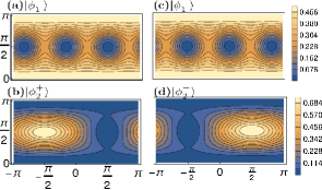
Figure 2: Husimi (quasiprobability distribution, $|\langle\phi_{i}|\theta_{0},\phi_{0}\rangle|^{2}$) plots for a set of four three-qubit bases states ($|\phi_{i}\rangle$), where $|\theta_{0},\phi_{0}\rangle$ is an arbitrary three-qubit, parametrized by ($\theta_{0},\phi_{0}$).

In this basis, the unitary operator $\mathcal{U}$ is given by

$$\mathcal{U}=\begin{pmatrix}\mathcal{U}_{+}&0\\ 0&\mathcal{U}_{-}\end{pmatrix},$$ (10)

where $0$ is a $2\times 2$ null matrix, and $2\times 2$-dimensional blocks $\mathcal{U}_{+}$ ($\mathcal{U}_{-}$) are written the bases $\{\phi_{1}^{+},\phi_{2}^{+}\}$ ($\{\phi_{1}^{-},\phi_{2}^{-}\}$), are in the positive (negative)-parity subspaces respectively. Explicitly, these have matrix elements

$$\mathcal{U}_{\pm}=\pm e^{\mp\frac{i\pi}{4}}e^{-i\kappa}\begin{pmatrix}\frac{i}{2}e^{-2i\kappa}&\mp\frac{\sqrt{3}}{2}e^{-2i\kappa}\\ \pm\frac{\sqrt{3}}{2}e^{2i\kappa}&-\frac{i}{2}e^{2i\kappa}\end{pmatrix}.$$ (11)

For simplicity the parameter $\kappa=\kappa_{0}/6$ is used in these expressions. Expressing $\mathcal{U}_{+}$ as a rotation $e^{-i\gamma\vec{\sigma}\cdot\hat{\eta}}$ by angle $\gamma$ about an axis $\hat{\eta}=\sin{\theta}\cos{\phi}\,\hat{x}+\sin{\theta}\sin{\phi}\,\hat{y}+\cos{\theta}\,\hat{z}$, upto a phase. On comparison with Eq. (11), we obtain, $\cos{\gamma}=\frac{1}{2}\sin{2\kappa}$, $\phi=\pi/2+2\kappa$, and $\sin{\theta}\sin{\gamma}=\sqrt{3}/2$. To evolve initial states we need $\mathcal{U}^{n}$ and therefore $\mathcal{U}_{\pm}^{n}$, which is explicitly given by,

$$\mathcal{U}_{\pm}^{n}=(\pm 1)^{n}e^{-in(\pm\frac{\pi}{4}+\kappa)}\begin{pmatrix}\alpha_{n}&\mp\beta_{n}^{*}\\ \pm\beta_{n}&\alpha_{n}^{*}\end{pmatrix},$$ (12)

where,

$$\alpha_{n} = T_{n}(\chi)+\frac{i}{2}\,U_{n-1}(\chi)\cos 2\kappa\quad\textrm{and}$$ (13)

$$\beta_{n} = (\sqrt{3}/2)\,U_{n-1}(\chi)\,e^{2i\kappa}.$$ (14)

The Chebyshev polynomials $T_{n}(\chi)$ and $U_{n-1}(\chi)$ are defined as $T_{n}(\chi)=\cos(n\gamma)$ and $U_{n-1}(\chi)=\sin(n\gamma)/\sin\gamma$ mason2002chebyshev with $\chi=\cos{\gamma}=\sin(2\kappa)/2$. Also note that $|\alpha_{n}|^{2}+|\beta_{n}|^{2}=1$. This follows both from the unitarity of $\mathcal{U}_{\pm}$ as well as a polynomial Pell identity satisfied by the Chebyshev polynomials, namely

$$T^{2}_{n}(x)+(1-x^{2})U_{n-1}^{2}(x)=1.$$ (15)

Remarkably, one can also view this as a new proof of the Pell identity satisfied by Chebyshev polynomials through the unitarity of quantum mechanics.

Note also that the range of $\chi$ is restricted in this case to $|\chi|\leq 1/2$, which in addition to the general identity $|T_{n}(\chi)|\leq 1$, also implies that $|U_{n-1}(\chi)|\leq 2/\sqrt{3},$ which follows from Eq. (14).

It is now straightforward to do time evolution, for an arbitrary three-qubit permutation symmetric state, and thereafter study its various properties. We further analyse two widely different three-qubit states ((i) $|0,0\rangle$ and (ii) $|\pi/2,-\pi/2\rangle$) in detail. For these two states, we obtain the exact expressions for linear entropy of a single-party reduced density matrix, time-average of the linear entropy, and concurrence between any two qubits as a measure of entanglement. These analytical expressions are verified numerically and also compared, where possible, with the data from the superconducting transmon qubits experiment of Neill16 . We particularly considered these two examples due to their preferential behaviors as classical phase space structures. A three-qubit state $\otimes^{3}|0\rangle$ corresponds to coherent state at $|0,0\rangle$ which is on the period-4 orbit whose classical correspondence is shown with a square in Fig. (1), while $\otimes^{3}|+\rangle_{y}$ corresponds to the coherent state at $|\pi/2,-\pi/2\rangle$, which is a fixed point on the classical phase space. This becomes unstable as we move from regular to mixed phase space at $\kappa_{0}=2$ and is indicated by a circle in Fig. (1).

II.1 Initial state $|000\rangle=|\theta_{0}=0,\phi_{0}=0\rangle$

Let us consider the state on the period-4 orbit, corresponding to the coherent state at $|0,0\rangle$ which is $\otimes^{3}|0\rangle$.

$$\begin{split}|\psi_{n}\rangle&=\mathcal{U}^{n}|000\rangle=\frac{1}{\sqrt{2}}\mathcal{U}^{n}\left(|\phi_{1}^{+}\rangle+|\phi_{1}^{-}\rangle\right)\\ &=\frac{1}{\sqrt{2}}\left(\mathcal{U}_{+}^{n}|\phi_{1}^{+}\rangle+\mathcal{U}_{-}^{n}|\phi_{1}^{-}\rangle\right)\\ &=\frac{1}{2}e^{-in\left(\frac{3\pi}{4}+\kappa\right)}\left\{(1+i^{n})\left(\alpha_{n}|000\rangle+i\beta_{n}|\overline{W}\rangle\right)\right.\\ &\left.+(1-i^{n})\left(i\alpha_{n}|111\rangle-\beta_{n}|W\rangle\right)\right\}.\end{split}$$ (16)

From this the $1$ and $2$ qubit reduced density matrices $\rho_{1}(n)=\text{tr}_{2,3}(|\psi_{n}\rangle\langle\psi_{n}|)$, $\rho_{12}(n)=\text{tr}_{3}(|\psi_{n}\rangle\langle\psi_{n}|)$ are obtained. The entanglement of one qubit with the other two is found as the linear entropy $1-{\rm{Tr}}\,[\rho_{1}(n)^{2}]$, and from the $2$-qubit reduced matrix, the entanglement between two qubits is found as the concurrence Wootters .

II.1.1 The linear entropy

It turns out that for even values of the time $n$, say $n=2m$, $\rho_{1}(2m)$ is diagonal, whose diagonal elements are, $\lambda(2m,\kappa_{0})$ and $1-\lambda(2m,\kappa_{0})$, from which the linear entropy,

$$S_{(0,0)}^{(3)}(2m,\kappa_{0})=2\lambda(2m,\kappa_{0})(1-\lambda(2m,\kappa_{0})),$$ (17)

where the eigenvalue,

$$\lambda(2m,\kappa_{0})=\frac{1}{2}U^{2}_{2m-1}(\chi)=\frac{2}{3}|\beta_{2m}|^{2}.$$ (18)

For odd values of $n$, $\rho_{1}(n)$ is not diagonal, but a peculiar result is obtained. One can evolve the even $n=2m$ states one step backward in time

$$|\phi_{2m-1}\rangle=\mathcal{U}^{-1}|\phi_{2m}\rangle,$$ (19)

where $\mathcal{U}$ is the Floquet operator in Eq. (7). Let $m$ itself be an even integer, which implies that only the first half of the state in Eq. (16) survives. Then upto an overall phase, using the nonlocal part of the unitary operator $\mathcal{U}$, the state upto local unitary operations is

$$|\phi_{2m-1}\rangle \stackunder{=}{\text{loc}} e^{i\kappa(\sigma_{1}^{z}\sigma_{2}^{z}+\sigma_{2}^{z}\sigma_{3}^{z}+\sigma_{3}^{z}\sigma_{1}^{z})}\left(\alpha_{2m}|000\rangle+i\beta_{2m}|\overline{W}\rangle\right),$$ (20)

$$= e^{3i\kappa}\alpha_{2m}|000\rangle+ie^{-i\kappa}\beta_{2m}|\overline{W}\rangle,$$

$$= \mathcal{V}\otimes\mathcal{V}\otimes\mathcal{V}|\phi_{2m}\rangle,$$

where single qubit unitary operator $\mathcal{V}=e^{i\kappa\sigma_{z}}$. Thus the three qubit state $|\psi_{2m-1}\rangle$, after odd numbered implementations of the unitary operator $\mathcal{U}$ are local unitarily equivalent to the state obtained after $2m$ implementations of $\mathcal{U}$ and hence all entanglement properties including entropy and concurrence are left unchanged for an odd-to-even time step. A similar situation holds when $m$ is odd. Therefore for a pair of consecutive implementations, entanglement among the qubits does not change, giving rise to step like features in the variation of entropy and concurrence with time. In particular

$$S_{(0,0)}^{(3)}(2n-1,\kappa_{0})=S_{(0,0)}^{(3)}(2n,\kappa_{0}),\;\;n=1,2,\cdots.$$ (21)

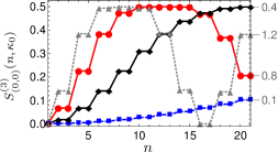
Figure 3: Linear entropy of a single qubit reduced state versus $n$ is plotted for initial state $|000\rangle$ at different values of $\kappa_{0}=0.1,\;0.4,\;0.8$ and $1.2$ as labelled on the right end of each curve.

This step like feature in the variation of entropy is illustrated for a few values of $\kappa_{0}$ in Fig. (3). It is seen that there is a monotonic increase of the initial rate of entropy production as a function of $\kappa_{0}$. This gives way to non-monotonic behavior both in time and in the parameter $\kappa_{0}$. The initial rate can be simply quantified by the entanglement entropy at $n=1$. Again using the linear entropy we have as a special case that

$$S_{(0,0)}^{(3)}(1,\kappa_{0})=\sin^{2}(\kappa_{0}/3)\left(1-\frac{1}{2}\sin^{2}(\kappa_{0}/3)\right),$$ (22)

which increases monotonically till $\kappa_{0}=3\pi/2$ where acquires the maximum value of $1/2$ which is also the upper-bound. We will see that the case of $\kappa_{0}=3\pi/2$ is one of maximal chaos in some sense for $j=3/2$.

For small $\kappa_{0}$, the growth of the entropy is $S_{(0,0)}^{(3)}(1,\kappa_{0})\approx\kappa_{0}^{2}/9$. From Fig. (3) it is seen that even for small values of $\kappa_{0}$ the entropy eventually becomes large and the maximum allowed value of $1/2$ is reached. As the classical dynamics for small $\kappa_{0}$ is regular, the large value of the entanglement reached is intriguing. We now estimate the time it takes for the entanglement to reach nearly the maximum value. The state in Eq. (16) clearly distinguishes times modulo 4. If the time $n$ is odd and $\beta_{n}$ vanishes (the conditions under which this happens is discussed below), the resultant state is the GHZ one with an equal superposition of $|000\rangle$ and $|111\rangle$ which is such that the reduced density matrices are maximally mixed and hence have maximum entropy. If the time $n$ is even and $\beta_{n}$ vanishes, there is no entanglement as the state becomes a tensor product, this also being apparent from the Eqs. (17) and  (18).

From Eq. (14), the vanishing of $\beta_{n}$ corresponds to the zeros of the Chebyshev polynomials of the second kind, $U_{n-1}(\chi)$, which are at $\chi=\chi_{k}=\cos(\pi k/n)$ and $k=1,2,\cdots,n-1$. Thus we are looking for values of $n$ such that

$$\frac{1}{2}\sin(\kappa_{0}/3)=\cos(\pi k/n),$$ (23)

which may be found from the continued fraction convergents of $r=\cos^{-1}[\sin(\kappa_{0}/3)/2]/\pi$. For small $\kappa_{0}$ ($\ll 1$), $r\lesssim 1/2$ the first non-zero convergent is $1/2$ and therefore the second is of the form $a_{1}/(2a_{1}+1)$ where $a_{1}$ is an integer. Identifying this with $k/n$ we see that $n$ is an odd integer and hence this corresponds to the case of maximum, or at least near-maximum, entanglement. Taylor expanding the $\sin$ and the $\cos^{-1}$ and retaining the lowest order terms then gives an estimate of the time $n_{*}$ at which the entanglement, for the first time, reaches nearly the maximum as

$$n_{*}\approx 2\left[\dfrac{3\pi}{2\kappa_{0}}-\frac{1}{2}\right]+1\approx\left[\frac{3\pi}{\kappa_{0}}\right],$$ (24)

and the time at which it gets unentangled, for the first time, is $\sim 2n_{*}$. We see from Fig. (3) that these are excellent estimates even when $\kappa_{0}$ is as large as $0.4$ or $0.8$.

The formation of non-classical states such as the GHZ in this instance is a forerunner of dynamical tunneling as for small $\kappa_{0}$ the islands at the “poles” of the phase space sphere can start to localize states for large values of $j$. This effect is seen prominently in the long-time averages. The intriguing increase of entanglement with time, even for small $\kappa_{0}$ in these states therefore has very different origins than the non-integrability of the kicked top.

II.1.2 Long time averaged linear entropy

The infinite time average of the linear entropy, which can be easily obtained from Eq. (17), maybe inaccessible experimentally but is of definite interest from the point of view of thermalization and it also is a way to study the influence of the parameter $\kappa_{0}$ directly. We need to use only even values of the time as for this state due to the property discussed above. We have

$$S^{(3)}_{(0,0)}(2m,\kappa_{0}) = U^{2}_{2m-1}(\chi)-\frac{1}{2}U^{4}_{2m-1}(\chi)$$ (25)

$$= \frac{\sin^{2}2m\gamma}{\sin^{2}\gamma}-\frac{1}{2}\frac{\sin^{4}2m\gamma}{\sin^{4}\gamma}.$$ (26)

The time-averaged linear entropy is thus given by

$$\langle S^{(3)}_{(0,0)}(\kappa_{0})\rangle = \lim_{N\rightarrow\infty}\frac{1}{N}\sum_{m=0}^{N-1}S^{(3)}_{(0,0)}(2m,\kappa)$$ (27)

$$= \frac{1}{2\sin^{2}\gamma}-\frac{3}{16\sin^{4}\gamma},$$ (28)

where we have used that $\langle\sin^{2}(2m\gamma)\rangle=1/2$ and $\langle\sin^{4}(2m\gamma)\rangle=3/8$, assuming that $\gamma\neq 0,\pi/2,\pi$. Further, using $\cos\gamma=\frac{1}{2}\sin 2\kappa=\frac{1}{2}\sin(\kappa_{0}/3)$, we obtain the average explicitly in terms of $\kappa_{0}$ as

$$\langle S^{(3)}_{(0,0)}(\kappa_{0})\rangle=\frac{5-2\sin^{2}(\kappa_{0}/3)}{\left(4-\sin^{2}(\kappa_{0}/3)\right)^{2}},\,0<\kappa_{0}<3\pi.$$ (29)

This attains its maximum value of $1/3$ at $\kappa_{0}=3\pi/2$. This may be used as a probe to understand the process of thermalization, which is discussed later in this section. However it is appropriate to point out that $\langle S^{(3)}_{(0,0)}(\kappa_{0})\rangle$ is discontinuous at $\kappa_{0}=0$ as it vanishes at $\kappa_{0}=0$ but is $5/16$ for arbitrarily small and nonzero values. Thus in this deep quantum regime, the state that starts off from the period-4 orbit gets entangled to a large extent even when the oribit is classically stable. However this is reflected in the infinite time average which includes highly nonclassical time scales, as discussed above.

II.1.3 Concurrence

While the linear entropy is a measure of entanglement of one qubit with the other two, the entanglement between any two qubits is quantified by the concurrence. Due to the permutation symmetry in the state it does not matter which two qubits are considered, there is only one concurrence. The concurrence is derived from the two-qubit reduced density matrix, as opposed to the entanglement of one qubit which needs only the one-qubit state. If $\rho_{12}$ is the two-qubit state, then its concurrence is given by

$$\mathcal{C}(\rho_{12})=\text{max}\left(0,\sqrt{\lambda_{1}}-\sqrt{\lambda_{2}}-\sqrt{\lambda_{3}}-\sqrt{\lambda_{4}}\right),$$ (30)

where $\lambda_{i}$ are eigenvalues in decreasing order of $(\sigma_{y}\otimes\sigma_{y})\rho_{12}(\sigma_{y}\otimes\sigma_{y})\rho_{12}^{*}$, where $\rho_{!2}^{*}$ is conjugation is in the standard ($\sigma_{z}$) basis.

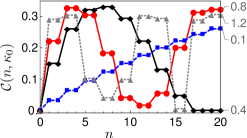
Figure 4: Concurrence of a two-qubit reduced state versus $n$ is plotted for $\kappa_{0}=0.1,\;0.4,\;0.8$ and $1.2$ as labelled on the right end of each curve.

An exact expression for concurrence amongst any two qubits in the state $|\psi_{n}\rangle$ of Eq. (16) is possible to obtain explicitly as the two-qubit state is an “$X$ state” YuEberly2007 when the time $n$ is even. A two-qubit reduced density operator of $\rho_{12}(n)$ obtained by tracing out one of the qubits in $|\psi_{n}\rangle\langle\psi_{n}|$ is given by,

$$\rho_{12}(n)=\begin{pmatrix}|\alpha_{n}|^{2}&0&0&-\frac{i}{\sqrt{3}}\alpha_{n}\beta_{n}^{*}\\ 0&\frac{1}{3}|\beta_{n}|^{2}&\frac{1}{3}|\beta_{n}|^{2}&0\\ 0&\frac{1}{3}|\beta_{n}|^{2}&\frac{1}{3}|\beta_{n}|^{2}&0\\ \frac{i}{\sqrt{3}}\alpha_{n}^{*}\beta_{n}&0&0&\frac{1}{3}|\beta_{n}|^{2}\end{pmatrix},$$ (31)

whose concurrence is found from the general formula for the $X$ states YuEberly2007 ,

$$\begin{split}&\mathcal{C}(n,\kappa_{0})=\\ &2\,\text{max}\left[0,\frac{1}{3}|\beta_{n}|^{2}-\frac{1}{\sqrt{3}}|\alpha_{n}||\beta_{n}|,-(\frac{1}{3}|\beta|_{n}^{2}-\frac{1}{\sqrt{3}}|\alpha_{n}||\beta_{n}|)\right]\\ &=2\left|\frac{1}{3}|\beta_{n}|^{2}-\frac{1}{\sqrt{3}}|\alpha_{n}||\beta_{n}|\right|\\ &=\left|U_{n-1}(\chi)\right|\left|\frac{1}{2}|U_{n-1}(\chi)|-\sqrt{1-\frac{3}{4}|U_{n-1}(\chi)|^{2}}\right|,\end{split}$$ (32)

where we recall for convenience that $\chi=\cos\gamma=\sin(2\kappa)/2=\sin(\kappa_{0}/3)/2$. This is valid when the time $n$ is even,but from the arguments presented in the discussion of the entanglement entropy it follows that

$$\mathcal{C}(2m-1,\kappa_{0})=\mathcal{C}(2m,\kappa_{0}),\,m=1,2,\cdots.$$ (33)

See Fig. (4) for the variation of the concurrence with time for the same values of $\kappa_{0}$ as used in the previous figure. As with the case of the linear entropy, the concurrence initially increases monotonically with $\kappa_{0}$ as well as with time. Once again it is of interest to see how much concurrence is produced in simply the first step and this is

$$\mathcal{C}(1,\kappa_{0})=\sin(\kappa_{0}/3)\left[\sqrt{1-\frac{3}{4}\sin^{2}(\kappa_{0}/3)}-\frac{1}{2}\sin(\kappa_{0}/3)\right],$$ (34)

which is valid when $0\leq\kappa_{0}\leq 3\pi$, and beyond this the concurrence is periodic. Interestingly this is monotonic in $\kappa_{0}$ only till $\kappa_{0}=\pi/2$, where it attains the maximum value of $(\sqrt{13}-1)/8\approx 0.3257$. This is in contrast to the linear entropy or entanglement of one qubit with the rest which grows till $\kappa_{0}=\pi$.

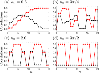
Figure 5: Solid curve with circles and dashed curve with squares show the variation of entropy of a single qubit reduced state and concurrence between a pair of two qubits respectively, with $n$ as three-qubit initial state $|000\rangle$ evolves under $\mathcal{U}^{n}$. Parts (a), (b), (c), and (d) correspond to different values of chaoticity parameter ($\kappa_{0}$) as mentioned.

It is useful to compare the concurrence and entanglement entropy directly and this is illustrated in Fig. (5) where for $4$ value of $\kappa_{0}$ these are plotted as a function of time. It is seen that while initially both of them grow, after a certain time, the concurrence starts to decrease while the entanglement continues to increase. This is the phase where entanglement is started to be shared globally rather than in bipartite manner. In this case of only $3$ qubits, this implies that tripartite entanglement starts to significantly grow after this time. It is also seen that when the entanglement entropy is the maximum possible, concurrence is at a minimum, and sometimes vanishes. This is consistent with the fact that entanglement is monogamous and hence cannot be simultaneously shared among the three qubits. It is interesting that the simple formulas derived for this system illustrates these more general features. In particular it is clear from Eq. (17) and Eq. (32) that while both the entanglement and concurrence vanish when $U_{n-1}(\chi)=0$, the concurrence also vanishes when $U_{n-1}(\chi)=\pm 1$, a case that corresponds to a maximum entanglement. More discussion on this is also found in Madhok2018_corr .

A curious case is obtained when $\kappa_{0}=3\pi/2$ when $\cos\gamma=1/2$ and hence $\gamma=\pi/3$ and $U_{n-1}(\chi)=\sin(2\pi n/3)/\sin(\pi/3)$, which takes the value $0$ when $n\,(\text{mod}\,3)=0$, is $+1$ when $n\,(\text{mod}\,3)=1$ and is $-1$ when $n\,(\text{mod}\,3)=2$. This implies that when $n\,(\text{mod}\,6)\neq 0$ or $-1$ the entanglement entropy is the maximum possible value of $1/2$ while the concurrence vanishes for all values of time $n$, as seen in the last panel of Fig. (5). Thus in this case the entanglement is shared only in a tripartite manner. We will return to this case later, but note here that indeed special values of such parameters in Floquet spin systems display similar behavior with large multipartite entanglement SunilMishraArulSubhra .

II.2 Initial state $|+++\rangle_{y}=|\theta_{0}=\pi/2,\phi_{0}=-\pi/2\rangle$ and beyond

We considered in some detail the fate of the state $|000\rangle$, we now study the case of the three-qubit state $|\psi_{0}\rangle=|+++\rangle_{y}$, where $|+\rangle_{y}=\frac{1}{\sqrt{2}}(|0\rangle+i|1\rangle)$ is an eigenvector of $\sigma_{y}$ with eigenvalue $+1$. The former is an eigenstate of the interaction term in the Floquet operator $\mathcal{U}$, while the latter is the eigenstate of the field. When $|+++\rangle_{y}$ is the initial state, it’s evolution lies entirely in the positive parity sector as it can be also written as $\otimes^{3}|+\rangle_{y}=(|\phi_{1}^{+}\rangle+\sqrt{3}i|\phi_{2}^{+}\rangle)/2$. As a coherent state it corresponds to being localized at $|\pi/2,-\pi/2\rangle$. The corresponding classical object is a fixed point that is stable till $\kappa_{0}=2$. The time evolved state is then

$$|\psi_{n}\rangle=\mathcal{U}^{n}|+++\rangle_{y}=e^{-in(\frac{\pi}{4}+\kappa)}\left(\gamma_{n}|\phi_{1}^{+}\rangle+\delta_{n}|\phi_{2}^{+}\rangle\right),$$ (35)

where $\gamma_{n}=(\alpha_{n}-i\sqrt{3}\beta_{n}^{*})/2$ and $\delta_{n}=(\beta_{n}+i\sqrt{3}\alpha_{n}^{*})/2$. and the $\alpha_{n}$ and $\beta_{n}$ are same as in Eq. (13).

One can obtain the single-party reduced state by tracing out any two-qubits, $\rho_{1}(n)=$

$$\begin{pmatrix}\frac{1}{2}&-\frac{i}{3}\left(|\delta_{n}|^{2}-\sqrt{3}\,\text{Im}(\gamma_{n}\delta_{n}^{*})\right)\\ \frac{i}{3}\left(|\delta_{n}|^{2}-\sqrt{3}\,\text{Im}(\gamma_{n}\delta_{n}^{*})\right)&\frac{1}{2}\end{pmatrix}.$$

(36)

The eigenvalues of $\rho_{1}(n)$ are simple and given by $2\chi^{2}U^{2}_{n-1}(\chi)$ and $1-2\chi^{2}U_{n-1}^{2}(\chi)$; hence the linear entropy is

$$S_{(\frac{\pi}{2},-\frac{\pi}{2})}^{(3)}(n,\kappa_{0})=4\chi^{2}U^{2}_{n-1}(\chi)\left(1-2\chi^{2}U_{n-1}^{2}(\chi)\right).$$ (37)

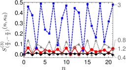
Figure 6: Linear entropy of a single qubit reduced state versus $n$ is plotted for different values of $\kappa_{0}$. Curves correspond to $\kappa_{0}=0.4,\;0.8,\;1.2$ and $3.0$ are shown by solid line with diamonds, solid line with circles, dashed line with triangles, and dashed line with squares respectively.

Figure (6) shows the growth of the entanglement entropy in this state as a function of time $n$ for four different values of $\kappa_{0}$. Comparing with Fig. (3) we see that the entanglement increases much more slowly, in keeping with the classical interpretation of this state as being localized on a fixed point. However the initial $n=1$ is the same in both the cases, $S^{(3)}_{(\frac{\pi}{2},-\frac{\pi}{2})}(1,\kappa_{0})$ is still given Eq. (22), and hence the entanglement after the first step is $\sim\kappa_{0}^{2}/9$ for small $\kappa_{0}$.

A difference is seen at $n=2$ when

$$S_{(\frac{\pi}{2},-\frac{\pi}{2})}^{(3)}(2,\kappa_{0})=\sin^{4}(\kappa_{0}/3)\left(1-\frac{1}{2}\sin^{4}(\kappa_{0}/3)\right),$$ (38)

thus while $S_{(0,0)}^{(3)}(2,\kappa_{0})=S_{(0,0)}^{(3)}(1,\kappa_{0})$, $S_{(\frac{\pi}{2},-\frac{\pi}{2})}^{(3)}(2,\kappa_{0})<S_{(\frac{\pi}{2},-\frac{\pi}{2})}^{(3)}(1,\kappa_{0}).$ In fact the contrast with the state $|000\rangle$ is most apparent when we observe that Eq. (37) implies that

$$S_{(\frac{\pi}{2},-\frac{\pi}{2})}^{(3)}(n,\kappa_{0})\leq 4\chi^{2}U_{n-1}^{2}(\chi)\leq\frac{4}{3}\sin^{2}(\kappa_{0}/3),$$ (39)

the last inequality is due to the upper-bound $|U_{n-1}(\chi)|\leq 2/\sqrt{3}$ which as has been observed above holds due to the restriction $|\chi|\leq 1/2$. This inequality is useful for small $\kappa_{0}$ in which case we have that $S_{(\frac{\pi}{2},-\frac{\pi}{2})}^{(3)}(n,\kappa_{0})\leq 4\kappa_{0}^{2}/27$, and is hence very close to the entanglement produced at the very first step, namely $\kappa_{0}^{2}/9$, and in particular has no secular growth towards large entanglement.

The long-time average value of the linear entropy is calculated exactly as the case when the initial state was $|000\rangle$, and we therefore merely display the result

$$\langle S^{(3)}_{(\frac{\pi}{2},-\frac{\pi}{2})}(\kappa_{0})\rangle=\frac{\sin^{2}(\kappa_{0}/3)}{\left(4-\sin^{2}(\kappa_{0}/3)\right)^{2}}\left(8-5\sin^{2}(\kappa_{0}/3)\right).$$ (40)

The major difference between the two initial states considered so far is apparent in this formula, as it is smooth at $\kappa_{0}=0$ and vanishes at $\kappa_{0}=0$, unlike the Eq. (29). The fact that the classical orbit in this case is a fixed point as opposed to a period-4 orbit is notable. In the case of the state $|000\rangle$, extremely non-classical states such as the GHZ can form at sufficiently long times and leads to the large average. We will see that the state centered at the fixed point can also have a large nonzero average for the case of $4$-qubits, again due to the formation of highly non-classical states mediated by tunneling.

Figure (7) shows the long-time average $\langle S^{(3)}_{(\theta_{0},\phi_{0})}(\kappa_{0})\rangle$ as a function of $\kappa_{0}$, for the case of 3-qubits, and three initial states, two of them being what we just discussed, namely $|000\rangle$ and $|+++\rangle_{y}$, which correspond to the cases with $\theta_{0}=0$ and $\pi/2$ respectively. That they are in some sense extreme cases is seen clearly in this figure. Each is seen to increase with the torsion $\kappa_{0}$ to $1/3$, while a state with $\theta_{0}=\pi/4$ (and in all cases $\phi_{0}=-\pi/2$) grows to $7/24$ which we will see is the lowest for any state. The average value of the linear entropy in the $N$-qubit permutation symmetric subspace SheshadriPRE2018 is given by

$$S_{RMT}(N)=\frac{N-1}{2N},$$ (41)

and for $N=3$ this also gives $1/3$. For at least three particular initial states, with important classical phase space correspondences, $|0,0\rangle\equiv|000\rangle$ and $|\pi/2,\pm\pi/2\rangle\equiv|\pm\pm\pm\rangle_{y}$ this value is, remarkably, exactly attained for $\kappa_{0}=3\pi/2$, as easily verified from Eq. (29) and Eq. (40). Thus ergodicity is attained as time averaged linear entropy approaches the state space averaged linear entropy.

Note that the $j=\infty$, classical system shows a transition to chaos in the same range of the parameter. While $j=3/2$ is too small to see effects such as the fixed points’ loss of stability, the overall region surrounding the classical fixed points $(\theta_{0},\phi_{0})=(\pi/2,\pm\pi/2)$ being stable for small $\kappa_{0}$ and gradually losing stability as the parameter is increased is reflected in the gradual increase of average entropy corresponding to the initial states $|\pi/2,\pm\pi/2\rangle$ starting from $0$ when $\kappa_{0}=0$. Notice that from a purely quantum mechanical view, $\otimes^{2j}|\pm\rangle_{y}$ are eigenstates of $\mathcal{U}$ at $\kappa_{0}=0$. In contrast, the initial state $|000\rangle$ corresponds to a classical period-4 orbit and assumes entanglement entropy as large as $5/16$ for arbitrarily small $\kappa_{0}$.

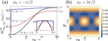
Figure 7: (a) Time averaged linear entropy, obtained over $n=1000$ periods, of a single qubit vs the parameter $\kappa_{0}$, for three initial coherent states $|\theta_{0},\phi_{0}\rangle$. The Eqs. (29, 40) apply to the curves labeled (1) and (3), as for $\theta_{0}=0$ the value of $\phi_{0}$ is immaterial on the sphere. Inset shows the entanglement periodicity in the parameter at $\kappa_{0}=3\pi$. Part (b) displays the time averaged linear entropy across all initial coherent states for the value $\kappa_{0}=3\pi/2$ and is described by Eq. (42).

II.2.1 Arbitrary initial states, $\kappa_{0}=3\pi/2$

For the 3-qubit case, the case of $\kappa_{0}=3\pi/2$ is an extreme one, and the eigenvalues of $\mathcal{U}$ in this case are $\exp(\pm 2\pi i/3)$ and $\pm\exp(\pm\pi i/6)$, implying that $\mathcal{U}^{12}=I$. Thus infinite time averages are finite ones over a period, in fact entanglement has a period of $6$ in this case and for arbitrary initial coherent states, the time-averaged entanglement entropy is obtained via a straightforward, if long, computation whose details we skip and state the result as

$$\begin{split}\langle S^{(3)}_{(\theta_{0},\phi_{0})}(3\pi/2)\rangle=&\frac{1}{48}[15+\cos(4\theta_{0})+\\ &(1+3\cos(2\theta_{0}))\sin^{4}\theta_{0}\sin^{2}(2\phi_{0})].\end{split}$$ (42)

This takes values in the narrow interval $[7/24,1/3]$, and is shown in Fig. (7). The minimum corresponds to several initial states including $|\pi/4,\pm\pi/2\rangle$ and the maximum includes the $|0,0\rangle$ and $|\pi/2,\pm\pi/2\rangle$ states as already noted above. The structures seen are not directly linked to classical phase space orbits, except through shared symmetries RuebeckArjendu2017 , and cannot be expected to do so as the classical limit is for fixed $\kappa_{0}$ and $j\rightarrow\infty$. Nevertheless these results lend quantitative credence to thermalization in the sense that the time averaged entropy of subsystems of most states are close to the ensemble average for suitable large $\kappa_{0}$, even for the 3-qubit case Neill16 ; Rigol16 .which, when $\kappa_{0}=3\pi/2$ approaches $1/3$. Coincidentaly, as mentioned above, this is same as the average linear entropy of a single qubit reduced state in a set of random symmetric three-qubit states. The calculations for the case of a general initial state and more figures of the long-time averages are presented in the Appendix.

III Comparison with an experiment

We analyse the data from a recent experiment Neill16 , that demonstrates the kicked top dynamics of a spin-$3/2$, using three superconducting transmon qubits. Experimental data corresponds to the two special initial states: $|0,0\rangle$ and $|\pi/2,-\pi/2\rangle$, (whose analytical solutions are given in sections II.1 and II.2 respectively), each one for two values of chaoticity parameter, $\kappa_{0}=0.5$ and $2.5$. Three-qubit state is experimentally initialized in given initial states (respectively), and then allowed to undergo a series of kicks and evolutions, separately for $\kappa_{0}=0.5$ and $2.5$, as described in Neill16 for a total of $20$ time steps.

Details of the analysis of the raw experimental data, which often has negative states, is outlined. We analysed the complete quantum state tomographic data, obtained at the end of each time step. State of a three-qubit system is obtained via complete quantum state tomography using a set of 64 projective measurements. These projective measurements are constructed by taking the combinations of Pauli-$x,y,z$ matrices ($\sigma_{x}$, $\sigma_{y}$ $\sigma_{z}$) and the Identity operator ($I$) james-pra-2001 ; Neill16 . These measurements are experimentally realized by various single qubit rotations ($\mathcal{R}$) followed by $\sigma_{z}$ measurements on individual qubits, that effectively performs a $\sigma_{i^{\prime}}$ measurement (for $i^{\prime}=x$, $\mathcal{R}=$Hadamard operator $(H_{d})$; $i^{\prime}=y$, $\mathcal{R}=$ Phase shift $(\mathcal{S}).H_{d}$; $i^{\prime}=z$, $\mathcal{R}=I$) Neill16 . Multiple implementations of each measurement, provides the relative occupancy of the eight basis states of a three-qubit system. The resulting relative populations ($p_{m}$) of these eight states are thus obtained experimentally.

In order to compensate the effect of errors induced by the measurements, the intrinsic populations ($p_{int}$) are obtained via a correction matrix ($F$) steffen-science-2006 ; lucero-prl-2008 . We have, $p_{int}=F^{-1}p_{m}$, where $F=F_{1}\otimes F_{2}\otimes F_{3}$. $F_{i}$ is the measurement error corresponding to $i^{th}$ qubit, given as,

$$F_{i}=\left(\begin{array}[]{cc}f_{0}^{(i)}&1-f_{1}^{(i)}\\ 1-f_{0}^{(i)}&f_{1}^{(i)}\end{array}\right).$$

Here, $f_{0}^{(i)}$ is the probability by which a state $|0\rangle$ of the $i^{th}$ qubit is correctly identified as $|0\rangle$, while $1-f_{1}^{(i)}$ is the probability by which, a state that is actually $|0\rangle$ is being wrongly considered as $|1\rangle$. $f_{0}^{(i)}$ and $f_{1}^{(i)}$ are termed as the measurement fidelities of the basis states $|0\rangle$ and $|1\rangle$ respectively of the $i^{th}$ qubit. Using a part of the measurement data corresponding to the initial state preparation, we estimated the measurement fidelities as $f_{0}^{(1)}=0.98$, $f_{1}^{(1)}=0.92$, $f_{0}^{(2)}=0.98$, $f_{1}^{(2)}=0.94$, $f_{0}^{(3)}=0.96$, $f_{1}^{(3)}=0.87$. The intrinsic populations obtained in this manner are positive (as observed till second decimal place). Using these intrinsic population values, three-qubit density operators are obtained, that further undergo the convex optimization. The fidelities between the theoretically expected ($\rho_{t}$) and the experimentally obtained ($\rho_{e}$) states is given by Neill16

$$\mathcal{F}=Tr\sqrt{\sqrt{\rho_{t}}\rho_{e}\sqrt{\rho_{t}}}.$$ (43)

These experimentally obtained three-qubit density operators are then used in our study to obtain the correlations, such as linear entropy of a single qubit reduced state and a two-qubit entanglement measure, concurrence.

Experimental data has its own imperfections, and the three-qubit experimental state may be not be permutation symmetric under qubit exchange. Therefore, corresponding to each three-qubit density operator, three single qubit reduced density operators (say $\rho_{1}$, $\rho_{2}$, $\rho_{3}$) and three two-qubit reduced density operators (say $\rho_{12}$, $\rho_{23}$, $\rho_{13}$) are obtained. At each time step, using various single qubit and two-qubit density operators correlations such as linear entropy and concurrence are calculated respectively and their average behavior is observed.

Figure 8 shows the comparison between the analytical results (dashed curves with markers) and those using experimental data from Neill16 , shown as solid curves with markers for $\kappa_{0}$= $0.5$ and $2.5$. Numerical results are also plotted as dashed curves in Fig. 8, but are naturally indistinct from the respective analytical results. More extensive analytical results have already been displayed in Figs. (3)- (6) and discussed in the previous section.

The Fig. (8(a,b)), corresponds to the initial state $|000\rangle$, whose classical limit is the period-4 orbit.This classical the period-4 orbit is unstable at $\kappa_{0}=2.5$ and we see a rapid growth in the entanglement. However even at $\kappa_{0}=0.5$ entanglement grows to near maximal values, consistent with the large time average in Eq. (29), and with the analysis that predicts that the maximum occurs at a time scale $n_{*}\sim 3\pi/\kappa_{0}\sim 19$. We also noted that the entanglement at time $2n$ is same as the entanglement at time $2n-1$, see Eqs. (21) and  (33). Interestingly these are quite remarkably present (but previously unnoticed) in the experimental data for the first few time steps. All entanglement properties including concurrence is left approximately unchanged in the experimental data for an odd-to-even time step as seen in Fig. (8(a,b)). The degradation of this phenomenon is naturally to be attributed to decoherence and maybe a good measure of it.

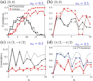
Figure 8: Plots showing analytical (dashed curves with markers), experimental (solid curves with markers) and numerical (dashed) curves of linear entropy and concurrence as a function of the number of kicks, as the initial state $|\psi_{0}\rangle$ is evolved under repeated applications of operator $\mathcal{U}$. Parameters of the initial state, $(\theta_{0},\phi_{0})$, and chaoticity parameter, $\kappa_{0}$, are specified in each figure. Analytical (wherever plotted) and numerical curves exactly overlap, and hence can not be seen separately.

The plots showing comparison of linear entropy and concurrence from the experimental data for the state $|\pi/2,-\pi/2\rangle$ when $\kappa_{0}=0.5$ and $\kappa_{0}=2.5$, are shown in Fig. (8(c,d)). It shows a much smaller entropy growth for $\kappa_{0}=0.5$ in comparison to the state $|000\rangle$, consistent with the bound in Eq. (39) and is a reflection, in the semiclassical limit, of the stable neighborhood of $|\pi/2,-\pi/2\rangle$. This is also consistent with the long time average, already displayed in Eq. (40). More qualitative discussions of the time-evolution have been published in Madhok2018_corr .

IV Exact solution for four-qubits:

It is particularly interesting to study a four-qubit kicked top as this is the smallest system where all-to-all interaction among qubits is different from that of nearest-neighbour interaction, and therefore presents a special case of a genuinely nonintegrable system. Surprisingly, even in this case, an exact solution to the kicked top with spin $j=2$, is possible. Similar to that of three-qubit kicked top, we are again confined to ($2j+1=5$)-dimensional permutation symmetric subspace of the total $2^{2j}=16$-dimensional Hilbert space. In this case the parity symmetry reduced and permutation symmetric basis in which $\mathcal{U}$ is block-diagonal is

$$|\phi_{1}^{\pm}\rangle = \frac{1}{\sqrt{2}}(|W\rangle\mp|\overline{W}\rangle),$$

$$|\phi_{2}^{\pm}\rangle = \frac{1}{\sqrt{2}}(|0000\rangle\pm|1111\rangle),\,\textrm{and}$$

$$|\phi_{3}^{+}\rangle = \frac{1}{\sqrt{6}}\sum_{\mathcal{P}}|0011\rangle_{\mathcal{P}}$$ (44)

where $|W\rangle=\frac{1}{2}\sum_{\mathcal{P}}|0001\rangle_{\mathcal{P}}$, $|\overline{W}\rangle=\frac{1}{2}\sum_{\mathcal{P}}|1110\rangle_{\mathcal{P}}$, and $\sum_{\mathcal{P}}$ sums over all possible permutations. Husimi plots for each of these states is shown in Fig. (9).

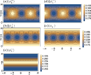
Figure 9: Husimi (quasiprobability distribution, $|\langle\phi_{i}|\theta_{0},\phi_{0}\rangle|^{2}$) plots for a set of five four-qubit bases states ($|\phi_{i}\rangle$), where $|\theta_{0},\phi_{0}\rangle$ is an arbitrary four-qubit, parametrized by ($\theta_{0},\phi_{0}$).

While all of these states $|\phi_{j}^{\pm}\rangle$ are eigenstates of the parity operator $\otimes^{4}_{j=1}\sigma^{y}_{j}$ with eigenvalue $\pm 1$, a peculiarity of 4-qubits is that $|\phi_{1}^{+}\rangle$ is also an eigenstate of the Floquet operator $\mathcal{U}$ with eigenvalue $-1$ for all values of the parameter $\kappa_{0}$.

Thus the $5-$ dimensional space splits into $1\oplus 2\oplus 2$ subspaces on which the operators are $\mathcal{U}_{0}=-1$ and $\mathcal{U}_{\pm}$. Note that we continue to use the same symbol for the symmetry reduced Floquet operators as for the 3-qubit case, although they are not the same. It is interesting that the eigenstate $|\phi_{1}^{+}\rangle$ still has a classically viable interpretation, but only for small $\kappa_{0}$, where as is clear from the Husimi, it is localized on the fixed points and the symmetric islands. A more detailed study of eigenstates is postponed while we concentrate here on the time evolution.

In this basis, the unitary Floquet operator $\mathcal{U}$ becomes block diagonal, which makes it easy to take the $n^{th}$ power of the unitary operator $\mathcal{U}$,

$$\mathcal{U}^{n}=\begin{pmatrix}(-1)^{n}&0&0\\ 0&\mathcal{U}_{+}^{n}&0\\ 0&0&\mathcal{U}_{-}^{n}\end{pmatrix}.$$ (45)

Thus in this case also we do not encounter the need to take powers of any matrix other than $2$-dimensional ones. Block $\mathcal{U}_{+}$ is $\mathcal{U}$ in the basis $\{\phi_{2}^{+},\phi_{3}^{+}\}$ and is,

$$\mathcal{U}_{+}=-ie^{-\frac{i\kappa}{2}}\left(\begin{array}[]{cc}\frac{i}{2}e^{-i\kappa}&\frac{\sqrt{3}i}{2}e^{-i\kappa}\\ \frac{\sqrt{3}i}{2}e^{i\kappa}&-\frac{i}{2}e^{i\kappa}\\ \end{array}\right),$$ (46)

while $\mathcal{U}_{-}$ is $\mathcal{U}$ in the basis $\{\phi_{1}^{-},\phi_{2}^{-}\}$,

$$\mathcal{U}_{-}=e^{-\frac{3i\kappa}{4}}\left(\begin{array}[]{cc}0&e^{\frac{3i\kappa}{4}}\\ -e^{-\frac{3i\kappa}{4}}&0\\ \end{array}\right),$$ (47)

where for simplicity we have used $\kappa=\kappa_{0}/2$.

Adopting the same procedure as for the case of 3 qubits, namely expressing $\mathcal{U}_{+}$ as a $SU(2)$ rotation, apart from a phase, and taking its power results in

$$\mathcal{U}_{+}^{n} = e^{-\frac{in(\pi+\kappa)}{2}}\begin{pmatrix}\alpha_{n}&i\beta_{n}^{*}\\ i\beta_{n}&\alpha_{n}^{*}\end{pmatrix},$$ (48)

where

$$\alpha_{n}=T_{n}(\chi)+\frac{i}{2}U_{n-1}(\chi)\cos{\kappa},\,\beta_{n}=\frac{\sqrt{3}}{2}U_{n-1}(\chi)e^{i\kappa}.$$ (49)

As above, $T_{n}(\chi)$ and $U_{n-1}(\chi)$ denote the Chebyshev polynomials of the first and second kinds respectively, but now $\chi=\sin{\kappa}/2=\sin(\kappa_{0}/2)/2$.

Similarly,

$$\mathcal{U}_{-}^{n}=e^{-\frac{3in\kappa}{4}}\left(\begin{array}[]{cc}\cos\frac{n\pi}{2}&e^{\frac{3i\kappa}{4}}\sin\frac{n\pi}{2}\\ -e^{-\frac{3i\kappa}{4}}\sin\frac{n\pi}{2}&\cos\frac{n\pi}{2}\\ \end{array}\right),$$ (50)

which has a much simpler form than the $\mathcal{U}_{+}^{n}$ and in fact $\mathcal{U}_{-}^{2}=-e^{-3i\kappa_{0}/4}I_{2}$ is up to a dynamical phase proportional to the identity. Thus all states in the negative parity subspace are essentially periodic with period-2, a uniquely quantum feature. In particular the GHZ state $|\phi_{2}^{-}\rangle=(|0000\rangle-|1111\rangle)/\sqrt{2}$ would be of this kind. Using these it is possible to find the exact evolution of the entanglement entropy of any one-qubit and again in particular we again concentrate on the initial states being $|0000\rangle$ and $|\pm\pm\pm\pm\rangle_{y}$, for the same reasons as in the 3 qubit case.

IV.1 Initial state $|\psi_{0}\rangle=|0000\rangle$

Considering four qubit state $|0000\rangle$, under the ‘$n$’ implementations of unitary operator $\mathcal{U}$,

$$\mathcal{U}^{n}|0000\rangle = \frac{1}{\sqrt{2}}\left(\mathcal{U}^{n}_{+}|\phi_{2}^{+}\rangle+\mathcal{U}^{n}_{-}|\phi_{2}^{-}\rangle\right).$$ (51)

leads to the state $|\psi_{n}\rangle$ at time $n$. Just as for the 3 qubit case the state $\mathcal{U}^{2n}|0000\rangle$ is upto local-unitary operators same as $\mathcal{U}^{2n-1}|0000\rangle$, and therefore again all entanglement properties have “steps” in their dynamical evolution and it is sufficient to consider the time $n$ to be an even integer. In this case

$$|\psi_{n}\rangle=e^{-\frac{in(\pi+\kappa)}{2}}\frac{1}{\sqrt{2}}\left(\alpha_{n}|\phi_{2}^{+}\rangle+i\beta_{n}|\phi_{3}^{+}\rangle+e^{-\frac{in\kappa}{4}}|\phi_{2}^{-}\rangle\right).$$ (52)

Single qubit reduced density matrix is simply diagonal for even values of $n$, eigenvalues being $\lambda(n,\kappa_{0})$ and $1-\lambda(n,\kappa_{0})$, where $\lambda(n,\kappa_{0})=\frac{1}{2}\left(1+\xi_{n}(\kappa_{0})\right)$, where

$$\xi_{n}(\kappa_{0}) = \textrm{Re}\left(\alpha_{n}e^{in\kappa_{0}/8}\right)$$

$$= T_{n}(\chi)\cos\frac{n\kappa_{0}}{8}-\frac{1}{2}U_{n-1}(\chi)\cos\frac{\kappa_{0}}{2}\sin\frac{n\kappa_{0}}{8}.$$

For even values of $n$, linear entropy of a single-qubit reduced state is given by,

$$S_{(0,0)}^{(4)}(n,\kappa_{0})=\frac{1}{2}\left[1-\xi_{n}^{2}(\kappa_{0})\right],$$ (54)

and at odd values, $S_{(0,0)}^{(4)}(2n-1,\kappa_{0})=S_{(0,0)}^{(4)}(2n,\kappa_{0})$. Figure (10) shows the evolution of this entanglement entropy for a few representative values of $\kappa_{0}$. In particular, even for $n=2$ (which is the same as $n=1$), we get a fairly long expression for the entanglement entropy, hence rather than display it, we state that for small $\kappa_{0}$ it increases as $S_{(0,0)}^{(4)}(1,\kappa_{0})\approx 3\,\kappa_{0}^{2}/32$, which is very similar to the corresponding 3-qubit case. It grows monotonically with $\kappa_{0}$ till $\kappa_{0}=\pi$ where it attains the upper-bound of $1/2$ already, in contrast to the 3-qubit case which attains this only at $\kappa_{0}=3\pi/2$.

Figure 10: Linear entropy of a single-qubit reduced state versus $n$ is plotted at different values of $\kappa_{0}$ shown in parts (a) and (b), corresponding to a four qubit initial state, $|0000\rangle$.

To find the relevant time scales in the growth of the entanglement, we note that the maximum value of the entropy is attained when $\xi_{n}(\kappa_{0})=0$. From Eq. (IV.1), and noting that the zeros of $T_{n}(\chi)$ and $U_{n-1}(\chi)$, do not occur simultaneously, we first examine the case when $n$ is even and $U_{n-1}(\chi)$ vanishes. This is similar to the analysis of the $3$ qubit case above and we simply state that this implies that $n_{*}\approx 4\pi/\kappa_{0}$. Thus the first even-time at which the second half of Eq. (IV.1) vanishes is $n_{*}$, however if this condition is satisfied the first part also vanishes as the $\cos(n\kappa_{0}/8)$ does. Thus the typical time-scale for the large entanglement to develop is slightly larger than the case of $3$ qubits where it was $3\pi/\kappa_{0}$. At the time when the entanglement is maximum, $\beta_{n}\approx 0$ and the resultant states are superpositions of $|\phi_{2}^{\pm}\rangle$ and are GHZ states. Thus the large 1-qubit entanglement observed in the experiment of Neill16 for $\kappa_{0}=0.5$ has more to do with the creation of such GHZ states than thermalization or chaos.

Long time average of the linear entropy is obtained by averaging over the time $n$, and is given by

$$\langle S^{(4)}_{(0,0)}(\kappa_{0})\rangle = \frac{1}{8}\left(\frac{9+2\cos^{2}(\kappa_{0}/2)}{3+\cos^{2}(\kappa_{0}/2)}\right),\kappa_{0}\neq 0,2\pi.$$ (55)

For $\kappa_{0}=0$, or $2\pi$, the entanglement vanishes. As soon as $\kappa_{0}$ becomes non-zero, this long-time averaged linear entropy attains a value of $2.75/8$, which further increases with $\kappa_{0}$ and attains a maximum value of $3/8$ at $\kappa_{0}=\pi$, as shown by the dashed curve in Fig. (11).

Thus, in this case, long time-averaged linear entropy of single-qubit reduced state oscillates within a very small interval of range $1/32$ for $\kappa_{0}\in(0,2\pi)$.

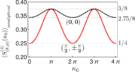
Figure 11: Analytically obtained expressions for time-averaged linear entropy for initial states $|0000\rangle$ (Eq. (55)) and $|++++\rangle_{y}$ (Eq. (59)) are plotted for $\kappa_{0}\in(0,4\pi)$. Extreme values are presented as horizontal lines, with their respective values ($S^{(4)}_{(\theta,\phi)}(\kappa_{0})=\textrm{constant}$) specified on the right side. Solid red curve and dashed black curve correspond to initial states $|++++\rangle_{y}$ and $|0000\rangle$ respectively.

IV.2 Initial state $|\psi_{0}\rangle=|++++\rangle_{y}$

This state lies entirely in the positive parity subspace of the five dimensional permutation symmetric space of four qubits, and is given by

$$\otimes^{4}|+\rangle_{y}=\frac{i}{\sqrt{2}}|\phi^{+}_{1}\rangle+\frac{1}{\sqrt{8}}|\phi_{2}^{+}\rangle-\sqrt{\frac{3}{8}}|\phi_{3}^{+}\rangle,$$ (56)

which under the action of $\mathcal{U}^{n}$, leads to $|\psi_{n}\rangle=\mathcal{U_{+}}^{n}|++++\rangle_{y}$, such that, (for $n>1$),

$$|\psi_{n}\rangle=\frac{(-1)^{n}}{\sqrt{2}}\left(i|\phi_{1}^{+}\rangle+e^{i\delta}\left(\alpha_{n}/2-i\sqrt{3}\beta_{n}^{*}/2\right)|\phi_{2}^{+}\rangle-e^{i\delta}\left(\sqrt{3}\alpha_{n}^{*}/2-i\beta_{n}/2\right)|\phi_{3}^{+}\rangle\right),$$ (57)

where $\delta=n(2\pi-\kappa_{0})/4$. The reduced density matrix of any one of the four qubits is given by,

$$\rho_{1}(n,\kappa_{0})=\textrm{Tr}_{2,3,4}\left(|\psi_{n}\rangle\langle\psi_{n}|\right)=\begin{pmatrix}1/2&\xi^{\prime}_{n}(\kappa_{0})\\ \xi^{\prime}_{n}(\kappa_{0})^{*}&1/2\end{pmatrix},$$ (58)

where,

$$\xi^{\prime}_{n}(\kappa_{0})=-i(T_{n}(\chi)\cos\delta+U_{n-1}(\chi)\sin\delta\cos(\kappa_{0}/2)),$$

and the linear entropy is given by

$$S^{(4)}_{(\pi/2,-\pi/2)}(n,\kappa_{0})=\frac{1}{2}\left(1-|\xi^{\prime}_{n}(\kappa_{0})|^{2}\right).$$

Figure (12) shows the evolution of this entanglement entropy for a few representative values of $\kappa_{0}$.

Figure 12: Linear entropy of a single-qubit reduced state versus $n$ is plotted at different values of $\kappa_{0}$ shown in parts (a), (b), (c), and (d), corresponding to a four qubit initial state, $|++++\rangle_{y}$.

A closed form expression for long time average linear entropy is then obtained as for the other case and results in (for $\kappa_{0}\neq 0,2\pi$),

$$\langle S^{(4)}_{(\frac{\pi}{2},\pm\frac{\pi}{2})}\rangle=\frac{1}{8}\left(\frac{9-\cos^{2}(\kappa_{0}/2)}{3+\cos^{2}(\kappa_{0}/2)}\right).$$ (59)

As soon as $\kappa_{0}$ becomes non-zero, this long time-averaged linear entropy attains its minimum value of $1/4$, which further increases with $\kappa_{0}$ and attains a maximum value of $3/8$ at $\kappa_{0}=\pi$, as shown by solid red curve in Fig. (11). In this case, long time-averaged linear entropy of single-qubit reduced state oscillates within a relatively larger interval of range $1/8$ for $\kappa_{0}\in(0,4\pi)$.

Time averaged linear entropy of single-qubit reduced state in both of these cases, reach their maximum value of $3/8$ when $\kappa_{0}=\pi$ and, remarkably, this matches with the average from the ensemble of random permutation symmetric states SheshadriPRE2018 of 4-qubits $S_{RMT}(4)$ as in the case of the 3-qubit case. In addition we see that the average for the states at $(\pi/2,\pm\pi/2)$ attain the value of $1/4$ for arbitrarily small $\kappa_{0}$ in contrast to the 3-qubit case which vanishes as in Eq. (40). In fact the non-zero average is seen in numerical calculations to be attained only on averaging over extremely long times for small $\kappa_{0}$, that reflects in Fig. (13), where different curves correspond to time-average over different times (as labelled in terms of $n$ in the inset). For small values of $\kappa_{0}$, i.e. $\kappa_{0}=2p\pi\pm\Delta\kappa_{0}$ ($p$ being an integer), time-average behavior of linear entropy for different times does not converge, and approaches the infinite-time average consistent with Eq. (59) and Fig. (11), as $n\rightarrow\infty$. This slow thermalization, specifically for state $|(\pi/2,\pm\pi/2)\rangle$ is attributed to the process of dynamical tunneling to which we now turn.

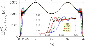
Figure 13: Simulated time-average linear entropy ($\langle S^{(4)}_{(\frac{\pi}{2},\pm\frac{\pi}{2})}(\kappa_{0})\rangle$) subject to initial state, $|(\pi/2,\pm\pi/2)\rangle$, plotted versus $\kappa_{0}$, is shown for different values of $n$ (as given in the inset) in the interval $\kappa_{0}\in[0,4\pi]$. Inset shows the blowed-up horizontal scale for $\kappa_{0}\in[0,\Delta\kappa_{0}]$, where $\Delta\kappa_{0}=2\pi/5$, that clearly presents the curves approaching the solid curve curve of Fig. 11.

IV.3 Dynamical tunneling

This very slow process is due to tunneling between $\otimes^{4}|+\rangle_{y}$ and $\otimes^{4}|-\rangle_{y}$. At $\kappa_{0}=0$, two positive parity eigenvectors of $\mathcal{U}$, $|\phi_{1}^{+}\rangle$ and $|\phi_{23}^{+}\rangle=\frac{1}{2}|\phi_{2}^{+}\rangle-\frac{\sqrt{3}}{2}|\phi_{3}^{+}\rangle$ are degenerate with eigenvalue $-1$. These can also be written as 4-qubit GHZ states GHZ0 ; GHZ :

$$i|\phi_{1}^{+}\rangle=\left(\otimes^{4}|+\rangle_{y}-\otimes^{4}|-\rangle_{y}\right)/\sqrt{2},$$ (60)

the unchanging eigenstate, and

$$|\phi_{23}\rangle=\left(\otimes^{4}|+\rangle_{y}+\otimes^{4}|-\rangle_{y}\right)/\sqrt{2}.$$ (61)

Thus

$$\mathcal{U}^{n}\otimes^{4}|+\rangle_{y}=(-1)^{n}\frac{i}{\sqrt{2}}|\phi_{1}^{+}\rangle+\mathcal{U}_{+}^{n}\frac{1}{\sqrt{2}}|\phi_{23}^{+}\rangle.$$ (62)

The eigenvalue of $\mathcal{U}_{+}$ that is $-1$ at $\kappa_{0}=0$ is $e^{i\gamma_{-}}$ with

$$\gamma_{-}=\frac{\kappa_{0}}{4}+\pi-\sin^{-1}\left(\frac{1}{2}\sin\frac{\kappa_{0}}{2}\right)\approx\pi-\frac{\kappa_{0}^{3}}{128}.$$ (63)

This implies that for $\kappa_{0}\ll 1$, the corresponding state and $|\phi_{1}^{+}\rangle$ are nearly degenerate. The splitting leads to a change in the relative phase of their contributions in Eq. (62) and at time $n_{*}\approx 128\pi/\kappa_{0}^{3}$ the evolved state is close to $\otimes^{4}|-\rangle$, leading to tunneling as shown in Fig. (14) between what in the classical limit are two stable islands. At time $n=n_{*}/2$ the state obtained is close to the GHZ state $(\otimes^{4}|+\rangle_{y}-i\otimes^{4}|-\rangle_{y})/\sqrt{2}$.

This tunneling is observed whenever $\otimes^{2j}|\pm\rangle$ are degenerate eigenstates of the rotation part of the Floquet $\mathcal{U}$. This implies that the number of qubits should be an integer multiple of $2\pi/p$, where $p$ is the rotation angle (we have used $p=\pi/2$, and hence the tunneling occurs when the number of qubits is a multiple of 4).

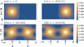
Figure 14: Husimi (quasi probability distribution) plots for the four-qubit initial state, $\otimes^{4}|+\rangle$, evolving under $n$ implementations of $\mathcal{U}$, and leading to tunneling to the state, $\otimes^{4}|-\rangle$, at time $n_{*}\approx 128\pi/\kappa_{0}^{3}\approx 402124$. ($\kappa_{0}=0.1$).

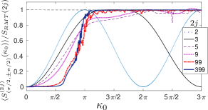
Figure 15: Normalized average single-qubit entanglement when the initial state is $\otimes^{2j}|+\rangle_{y}$ for increasing number of qubits (except multiples of $4$ where there is tunneling for $p=\pi/2$.)

For larger number of qubits, the average single-qubit entropy, normalized by the random state average, is numerically found when the initial state is $\otimes^{2j}|+\rangle_{y}$ and shown in Fig. (15). The number of qubits used for the cases shown in this figure are not multiples of $4$, and hence the long-time average vanishes at $\kappa_{0}=0$, that is there is no tunneling. The trend is in keeping with a more complex classical phase space that becomes fully chaotic when the random state average is approached. The initial state being centered on a fixed point, increasing the number of qubits leads to a sharp growth beyond $\kappa_{0}=2$ when the fixed point becomes unstable, a more detailed study of this is found in Bhosale-pre-2017 , without the connection to tunneling. Interestingly even for the 3-qubit case, for which we have the analytical evaluation in Eqs (40), a similar but smoother trend is displayed and reaches the random state value when $\kappa_{0}=3\pi/2$.

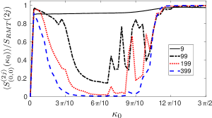
Figure 16: Normalized average single-qubit entanglement when the initial state is $\otimes^{2j}|0\rangle$ for increasing number of qubits.

The complementary state $\otimes_{k=1}^{2j}|0\rangle$ has a nonzero average as $\kappa_{0}$ approaches $0$, both for the 3- and the 4-qubit cases. We have already discussed the origin of this in some detail for the $3-$ qubit case. For a very large number of qubits we expect that classically the tunneling effect vanishes. This is borne out in Fig. (16), although surprisingly even for very large number of qubits for a range of $\kappa_{0}$ values close to $0$, the formation of nonclassical states resulting in large average single qubit entanglement is seen. The subsequent increase of entanglement for larger values of $\kappa_{0}$ is due to the destabilization of the period-4 orbit at $\kappa_{0}=\pi$. A more detailed analysis is called for, including the study of entanglement between large blocks of spins which will distinguish between the non-classical states produced when the system is near-integrable and the random states produced at much larger values of the parameter when the classical phase-space is mixed or chaotic. A recent analysis in kumari2018untangling uses an upper-bound of the entanglement entropy using the Fannes-Audernaert inequality to argue for connections between entanglement and chaos and why states localized on the stable period-4 orbits can have large entanglement in the deep quantum regime.

V Conclusions

Quest for an exactly solvable model is hard and often a matter of serendipity. In our work, we give exact solution for 3- and 4- qubit instances of the kicked top and explicitly derive expressions for the time evolved state, reduced density matrix, entanglement entropy and its long time average values. Our work provides interesting connections between a quantum system with few degrees of freedom and its classical limit that is non-integrable and can exhibit chaos for high $\kappa_{0}$ values. For example, we find that the exactly solvable 3- and 4- qubit instances of the kicked top provide insights into how entropy and entanglement thermalize in closed quantum systems in the sense of long time averages approaching ensemble averages, as the classical limit approaches global chaos, as predicted by random matrix theory. Since we derive exact analytical results valid for all values of $\kappa_{0}$, this will be further useful to study transition to thermalisation in closed quantum systems. Experiments have already probed the 3-qubit case, and it is worth mentioning that, in the light of our work, it should now be viewed as a study of thermalisation in an integrable system rather than thermalisation induced due to lack of sufficient number of conserved quantities Neill16 . It will be interesting to see at what spin size does the exact solvability of these models become intractable and whether or not that has a physical interpretation.

Even more remarkable is the entanglement dynamics at small values of the chaoticity parameter. This cannot be directly attributed to non-integrability. For example, even for small $\kappa_{0}$, in the case of the three qubit $|0,0\rangle$ state, we find an increase of entanglement with time, which can be attributed to the generation of highly non-classical GHZ type states. We accurately predict time scales for such entanglement dynamics and found an excellent agreement with the numerics. Likewise, the $|\pi/2,-\pi/2\rangle$ state in the 4-qubit case displays, for the same rotation angle, tunneling and creation of GHZ states and we have described this in detail as well. In the near-integrable regime we exactly calculate tunneling splitting and show this to be in agreement with the numerics. To the best of our knowledge, ours is the first work to find a connection between tunneling splitting, the number of qubits and a system parameter. It is worth mentioning that entanglement generation occurs despite the initial state being localised on a stable island with phase space having almost no chaos. We believe our findings and analysis of entanglement generation at low values of $\kappa_{0}$ will contribute to the understanding of entanglement generation in dynamical systems and it’s connections to classical bifurcations, emergence of structures and ergodicity in the phase space. This also complements our findings for higher values of $\kappa_{0}$ as well as the existing literature on the connections between entanglement generation and chaos.

Lastly, larger number of qubits can show genuine signatures of non-integrability and chaos, and tunneling leads to creation of macroscopic superpositions that are generalized GHZ states. We hope our work raises new questions and adds to the discussion on the connections between integrability, quantum chaos, and thermalization. Since the multi-qubit kicked top can be viewed as an analog quantum simulator, robustness of such a system to errors hauke2012can ; Shepelyansky_2001 , especially in the regime where we generate highly non-classical GHZ like states and explore truly quantum phenomena like tunneling, will be of interest to the quantum information community. As an aside, we are able to give an alternate proof of the Pell identity satisfied by the Chebyshev polynomials!

*

Appendix A Linear entropy of an arbitrary three-qubit permutation symmetric state

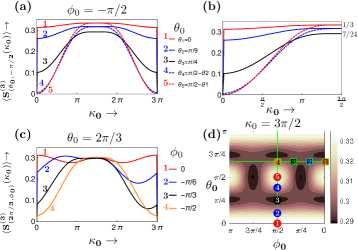
Figure 17: (a),(b) Time averaged linear entropy ($\langle S_{(\theta_{0},-\pi/2)}^{(3)}\rangle$) of a single party reduced state vs chaoticity parameter $\kappa_{0}$. Different curves correspond to different initial states, $|\theta_{0},-\pi/2\rangle$ as labelled $1$ to $5$, alongwith explicit values of $\theta_{0}$ given in the plot legends. These corresponding initial states $|\theta_{0},\phi_{0}\rangle$ are also marked as numbered circles in the contour plot given in part (d). Part (c) contains the plots for $\langle S_{(2\pi/3,\phi_{0})}^{(3)}\rangle$ vs chaoticity parameter $\kappa_{0}$ for a fixed value of $\theta_{0}=2\pi/3$. Different curves correspond to different initial states, labelled by numbers $1$ to $4$ alongwith explicit values of $\phi_{0}$ given in the plot legends. Respective initial states $|\theta_{0},\phi_{0}\rangle$ are also marked as numbered squares (with a green border) in the contour plot given in part (d). Contour plot shown in part (d) corresponds to $\kappa_{0}=3\pi/2$.

Considering a three-qubit state

$$|\psi_{0}\rangle=a_{1}|\phi_{1}^{+}\rangle+a_{2}|\phi_{2}^{+}\rangle+b_{1}|\phi_{1}^{-}\rangle+b_{2}|\phi_{2}^{-}\rangle.$$ (64)

Each of the three qubits are initialized in the same state ($|\psi\rangle=\cos\frac{\theta_{0}}{2}|0\rangle+e^{-i\phi_{0}}\sin\frac{\theta_{0}}{2}|1\rangle$, in the computational bases), such that the initial state of the $3-$ qubit system is $|\psi_{0}\rangle=\otimes^{3}|\psi\rangle$, where $\theta_{0}\in[0,\pi]$ and $\phi_{0}\in[-\pi,\pi]$. Repeated implementations of the unitary operator $\mathcal{U}$, leads to $|\psi_{n}\rangle=\mathcal{U}^{n}|\psi_{0}\rangle$. We obtain single-party reduced density operator by tracing out any of the two qubits of the three-qubit density operator ($\rho_{n}=|\psi_{n}\rangle\langle\psi_{n}|$), leading to,

$$\rho_{i}=\begin{pmatrix}r&s\\ s^{*}&1-r\end{pmatrix},$$ (65)

where the elements of the density operator are given by

$$r = \frac{1}{2}+\textrm{Re}\left(a_{1n}b_{1n}^{*}+\frac{1}{3}a_{2n}b_{2n}^{*}\right)\quad\textrm{and}$$

$$s = \frac{1}{\sqrt{3}}\textrm{Re}\left(a_{1n}b_{2n}^{*}+b_{1n}a_{2n}^{*}\right)+\frac{i}{\sqrt{3}}\textrm{Im}\left(a_{1n}a_{2n}^{*}+b_{1n}b_{2n}^{*}\right)$$ (66)

$$-\frac{i}{3}\left(a_{2n}+b_{2n}\right)\left(a_{2n}^{*}-b_{2n}^{*}\right).$$

Where the coefficients, $a_{1n}=a_{1}\alpha_{n}-a_{2}\beta_{n}^{*}$, $a_{2n}=a_{1}\beta_{n}+a_{2}\alpha_{n}^{*}$, $b_{1n}=i^{n}\left(b_{1}\alpha_{n}+b_{2}\beta_{n}^{*}\right)$, and $b_{2n}=i^{n}\left(b_{2}\alpha_{n}^{*}-b_{1}\beta_{n}\right)$. Linear entropy of the single-qubit (Eq. (65)) is thus given by,

$$S_{(\theta_{0},\phi_{0})}^{(3)}(n,\kappa)=2\left[r(1-r)-|s|^{2}\right].$$ (67)

Thus linear entropy is obtained as a function of the initial-state parameters ($\theta_{0},\phi_{0}$). Long time average linear entropy is calculated numerically with $n=1000$ for various initial states as shown in Fig. (17). Part (a) and (c) of Fig. (17) show the variation of time average entropy with chaoticity parameter for a period $2\pi j$. Pairs of complimentary $\theta_{0}$s, saturate to same values in the region around $\kappa_{0}=3\pi/2$. Part (b) of Fig. (17) highlights the range of values of average linear entropy at $\kappa_{0}=3\pi/2$, a scale of similar range in part (d) depicts that the linear entropy of a single-qubit reduced state for an arbitrary value of parameters ($\theta_{0},\phi_{0}$) fall into this range. Further, we have obtained an explicit closed form experssion for long time average linear entropy for an arbitrary ($\theta_{0},\phi_{0}$) at $\kappa_{0}=3\pi/2$, which is discussed in the main text.

References

- (1) Patrick Billingsley. Prime numbers and brownian motion. The American Mathematical Monthly, 80(10):1099–1115, 1973.
- (2) F. Haake. Quantum Signatures of Chaos. Spring-Verlag, Berlin, 1991.
- (3) Asher Peres. Quantum Theory: Concepts and Methods. Kluwer Academic Publishers, New York, 2002.
- (4) M Kuś, R Scharf, and F Haake. Symmetry versus degree of level repulsion for kicked quantum systems. Zeitschrift für Physik B Condensed Matter, 66(1):129–134, 1987.
- (5) M Kus, J Mostowski, and F Haake. Universality of eigenvector statistics of kicked tops of different symmetries. Journal of Physics A: Mathematical and General, 21(22):L1073, 1988.
- (6) K Zyczkowski. Indicators of quantum chaos based on eigenvector statistics. Journal of Physics A: Mathematical and General, 23(20):4427, 1990.
- (7) Peter Gerwinski, Fritz Haake, Harald Wiedemann, Marek Kuś, and Karol Życzkowski. Semiclassical spectra without periodic orbits for a kicked top. Phys. Rev. Lett., 74:1562–1565, Feb 1995.
- (8) Xiaoguang Wang, Shohini Ghose, Barry C. Sanders, and Bambi Hu. Entanglement as a signature of quantum chaos. Phys. Rev. E, 70:016217, 2004.
- (9) M. Lombardi and A. Matzkin. Entanglement and chaos in the kicked top. Phys. Rev. E, 83:016207, Jan 2011.
- (10) Shohini Ghose and Barry C. Sanders. Entanglement dynamics in chaotic systems. Phys. Rev. A, 70:062315, 2004.
- (11) Vaibhav Madhok, Carlos A. Riofrío, Shohini Ghose, and Ivan H. Deutsch. Information gain in tomography˘a quantum signature of chaos. Phys. Rev. Lett., 112:014102, 2014.
- (12) Angelo Piga, Maciej Lewenstein, and James Q. Quach. Quantum chaos and entanglement in ergodic and non-ergodic systems. arXiv preprint arXiv:1804.10543, 2018.
- (13) Udaysinh T. Bhosale and M. S. Santhanam. Signatures of bifurcation on quantum correlations: Case of the quantum kicked top. Phys. Rev. E, 95:012216, Jan 2017.
- (14) S. Chaudhury, A. Smith, B. E. Anderson, S. Ghose, and P. S. Jessen. Quantum signatures of chaos in a kicked top. Nature, 461:768, 2009.
- (15) C. Neill, P. Roushan, M. Fang, Y. Chen, M. Kolodrubetz, Z. Chen, A. Megrant, R. Barends, B. Campbell, B. Chiaro, A. Dunsworth, E. Jeffrey, J. Kelly, J. Mutus, P. J. J. O’Malley, C. Quintana, D. Sank, A. Vainsencher, J. Wenner, T. C. White, A. Polkovnikov, and J. M. Martinis. Ergodic dynamics and thermalization in an isolated quantum system. Nature Physics, 12:1037, 2016.
- (16) Amy C. Cassidy, Douglas Mason, Vanja Dunjko, and Maxim Olshanii. Threshold for chaos and thermalization in the one-dimensional mean-field bose-hubbard model. Phys. Rev. Lett., 102:025302, Jan 2009.
- (17) Lea F. Santos and Marcos Rigol. Onset of quantum chaos in one-dimensional bosonic and fermionic systems and its relation to thermalization. Phys. Rev. E, 81:036206, Mar 2010.
- (18) Luca D’Alessio, Yariv Kafri, Anatoli Polkovnikov, and Marcos Rigol. From quantum chaos and eigenstate thermalization to statistical mechanics and thermodynamics. Advances in Physics, 65(3):239–362, 2016.
- (19) R. V. Jensen and R. Shankar. Statistical behavior in deterministic quantum systems with few degrees of freedom. Phys. Rev. Lett., 54:1879–1882, Apr 1985.
- (20) J. M. Deutsch. Quantum statistical mechanics in a closed system. Phys. Rev. A, 43:2046–2049, 1991.
- (21) Mark Srednicki. Chaos and quantum thermalization. Phys. Rev. E, 50:888–901, 1994.
- (22) Marcos Rigol, Dunjko Vanja, and Olshanii Maxim. Thermalization and its mechanism for generic isolated quantum systems. Nature, 452(7189):854, 2009.
- (23) M. C. Bañuls, J. I. Cirac, and M. B. Hastings. Strong and weak thermalization of infinite nonintegrable quantum systems. Phys. Rev. Lett., 106:050405, Feb 2011.
- (24) J. M. Deutsch, Haibin Li, and Auditya Sharma. Microscopic origin of thermodynamic entropy in isolated systems. Phys. Rev. E, 87:042135, Apr 2013.
- (25) T Langen, R Geiger, M Kuhnert, B Rauer, and J Schmiedmayer. Local emergence of thermal correlations in an isolated quantum many-body system. Nature, 9:640, 2013.
- (26) Luca D’Alessio and Marcos Rigol. Long-time behavior of isolated periodically driven interacting lattice systems. Phys. Rev. X, 4:041048, Dec 2014.
- (27) Achilleas Lazarides, Arnab Das, and Roderich Moessner. Periodic thermodynamics of isolated quantum systems. Phys. Rev. Lett., 112:150401, Apr 2014.
- (28) Achilleas Lazarides, Arnab Das, and Roderich Moessner. Equilibrium states of generic quantum systems subject to periodic driving. Phys. Rev. E, 90:012110, Jul 2014.
- (29) Asmi Haldar, Roderich Moessner, and Arnab Das. Onset of floquet thermalization. Phys. Rev. B, 97:245122, Jun 2018.
- (30) Adam M. Kaufman, M. Eric Tai, Alexander Lukin, Matthew Rispoli, Robert Schittko, Philipp M. Preiss, and Markus Greiner. Quantum thermalization through entanglement in an isolated many-body system. Science, 353(6301):794–800, 2016.
- (31) Govinda Clos, Diego Porras, Ulrich Warring, and Tobias Schaetz. Time-resolved observation of thermalization in an isolated quantum system. Phys. Rev. Lett., 117:170401, Oct 2016.
- (32) Kaden R. A. Hazzard, Mauritz van den Worm, Michael Foss-Feig, Salvatore R. Manmana, Emanuele G. Dalla Torre, Tilman Pfau, Michael Kastner, and Ana Maria Rey. Quantum correlations and entanglement in far-from-equilibrium spin systems. Phys. Rev. A, 90:063622, Dec 2014.
- (33) M. C. Gutzwiller. Chaos in Classical and Quantum Mechanics. Springer-Verlag, New York, 1990.
- (34) Vaibhav Madhok, Shruti Dogra, and Arul Lakshminarayan. Quantum correlations as probes of chaos and ergodicity. Optics Communications, 420:189 – 193, 2018.
- (35) Emil A. Yuzbashyan and B. Sriram Shastry. Quantum integrability in systems with finite number of levels. Journal of Statistical Physics, 150(4):704–721, Feb 2013.
- (36) Paul A. Miller and Sarben Sarkar. Signatures of chaos in the entanglement of two coupled quantum kicked tops. Phys. Rev. E, 60:1542–1550, 1999.
- (37) Collin M Trail, Vaibhav Madhok, and Ivan H Deutsch. Entanglement and the generation of random states in the quantum chaotic dynamics of kicked coupled tops. Physical Review E, 78(4):046211, 2008.
- (38) Arul Lakshminarayan. Entangling power of quantized chaotic systems. Phys. Rev. E, 64:036207, 2001.
- (39) Jayendra N. Bandyopadhyay and Arul Lakshminarayan. Testing statistical bounds on entanglement using quantum chaos. Phys. Rev. Lett., 89:060402, 2002.
- (40) Jayendra N. Bandyopadhyay and Arul Lakshminarayan. Entanglement production in coupled chaotic systems : Case of the kicked tops. Phys. Rev. E, 69:016201, 2004.
- (41) A J Scott and Carlton M Caves. Entangling power of the quantum baker’s map. Journal of Physics A: Mathematical and General, 36(36):9553, 2003.
- (42) Arul Lakshminarayan, Shashi Srivastava, Roland Ketzmerick, Arnd Bäcker, and Steven Tomsovic. Entanglement and localization of eigenstates of interacting chaotic systems. Phys. Rev. E, 94:010205 (R), 2016.
- (43) Michael J. Davis and Eric J. Heller. Quantum dynamical tunneling in bound states. The Journal of Chemical Physics, 75(1):246–254, 1981.
- (44) W. A. Lin and L. E. Ballentine. Quantum tunneling and chaos in a driven anharmonic oscillator. Phys. Rev. Lett., 65:2927–2930, Dec 1990.
- (45) Asher Peres. Dynamical quasidegeneracies and quantum tunneling. Phys. Rev. Lett., 67:158–158, Jul 1991.
- (46) Steven Tomsovic, editor. Tunneling in complex systems. World Scientific, Singapore, 1998.
- (47) Srihari Keshavamurthy and Peter Schlagheck, editors. Dynamical Tunneling—Theory and Experiment. CRC Press, Boca Raton, FL, 2011.
- (48) G. J. Milburn. Simulating nonlinear spin models in an ion trap, 1999.
- (49) Joshua B. Ruebeck, Jie Lin, and Arjendu K. Pattanayak. Entanglement and its relationship to classical dynamics. Phys. Rev. E, 95:062222, 2017.
- (50) Udaysinh T. Bhosale and M. S. Santhanam. Periodicity of quantum correlations in the quantum kicked top. Phys. Rev. E, 98:052228, Nov 2018.
- (51) Tomaž Prosen. Exact time-correlation functions of quantum ising chain in a kicking transversal magnetic fieldspectral analysis of the adjoint propagator in heisenberg picture. Progress of Theoretical Physics Supplement, 139:191–203, 2000.
- (52) Arul Lakshminarayan and V. Subrahmanyam. Multipartite entanglement in a one-dimensional time-dependent ising model. Phys. Rev. A, 71:062334, Jun 2005.
- (53) Roy J. Glauber and Fritz Haake. Superradiant pulses and directed angular momentum states. Phys. Rev. A, 13:357, Oct 1976.
- (54) R. R. Puri. Mathematical Methods of Quantum Optics. Springer, Berlin, 2001.
- (55) John C Mason and David C Handscomb. Chebyshev polynomials. Chapman and Hall/CRC, 2002.
- (56) William K. Wootters. Entanglement of formation of an arbitrary state of two qubits. Phys. Rev. Lett., 80:2245–2248, 1998.
- (57) Ting Yu and J. H. Eberly. Evolution from entanglement to decoherence of bipartite mixed ”x” states. Quantum Info. Comput., 7(5):459–468, July 2007.
- (58) Sunil K. Mishra, Arul Lakshminarayan, and V. Subrahmanyam. Protocol using kicked ising dynamics for generating states with maximal multipartite entanglement. Phys. Rev. A, 91:022318, Feb 2015.
- (59) Akshay Seshadri, Vaibhav Madhok, and Arul Lakshminarayan. Tripartite mutual information, entanglement, and scrambling in permutation symmetric systems with an application to quantum chaos. Phys. Rev. E, 98:052205, Nov 2018.
- (60) Daniel F. V. James, Paul G. Kwiat, William J. Munro, and Andrew G. White. Measurement of qubits. Phys. Rev. A, 64:052312, 2001.
- (61) Matthias Steffen, M. Ansmann, Radoslaw C. Bialczak, N. Katz, Erik Lucero, R. McDermott, Matthew Neeley, E. M. Weig, A. N. Cleland, and John M. Martinis. Measurement of the entanglement of two superconducting qubits via state tomography. Science, 313(5792):1423–1425, 2006.
- (62) Erik Lucero, M. Hofheinz, M. Ansmann, Radoslaw C. Bialczak, N. Katz, Matthew Neeley, A. D. O’Connell, H. Wang, A. N. Cleland, and John M. Martinis. High-fidelity gates in a single josephson qubit. Phys. Rev. Lett., 100:247001, 2008.
- (63) Daniel M. Greenberger, Michael A. Horne, and Anton Zeilinger. Going Beyond Bell’s Theorem, pages 69–72. Springer Netherlands, Dordrecht, 1989.
- (64) Daniel M. Greenberger, Michael A. Horne, Abner Shimony, and Anton Zeilinger. Bell’s theorem without inequalities. American Journal of Physics, 58(12):1131–1143, 1990.
- (65) Meenu Kumari and Shohini Ghose. Untangling entanglement and chaos. arXiv preprint arXiv:1806.10545, 2018.
- (66) Philipp Hauke, Fernando M Cucchietti, Luca Tagliacozzo, Ivan Deutsch, and Maciej Lewenstein. Can one trust quantum simulators? Reports on Progress in Physics, 75(8):082401, 2012.
- (67) D. L. Shepelyansky. Quantum chaos and quantum computers. Physica Scripta, T90(1):112, 2001.