Robust Decision Trees Against Adversarial Examples

Abstract

Although adversarial examples and model robustness have been extensively studied in the context of linear models and neural networks, research on this issue in tree-based models and how to make tree-based models robust against adversarial examples is still limited. In this paper, we show that tree based models are also vulnerable to adversarial examples and develop a novel algorithm to learn robust trees. At its core, our method aims to optimize the performance under the worst-case perturbation of input features, which leads to a max-min saddle point problem. Incorporating this saddle point objective into the decision tree building procedure is non-trivial due to the discrete nature of trees—a naive approach to finding the best split according to this saddle point objective will take exponential time. To make our approach practical and scalable, we propose efficient tree building algorithms by approximating the inner minimizer in this saddle point problem, and present efficient implementations for classical information gain based trees as well as state-of-the-art tree boosting models such as XGBoost. Experimental results on real world datasets demonstrate that the proposed algorithms can substantially improve the robustness of tree-based models against adversarial examples.

1 Introduction

The discovery of adversarial examples in various deep learning models (Szegedy et al., 2013; Kos et al., 2018; Cheng et al., 2018; Chen et al., 2018a; Carlini & Wagner, 2018; Huang et al., 2017) has led to extensive studies of deep neural network (DNN) robustness under such maliciously crafted subtle perturbations. Although deep learning-based model robustness has been well-studied in the recent literature from both attack and defense perspectives, studies on the robustness of tree-based models are quite limited (Papernot et al., 2016a).

In our paper, we shed light on the adversarial robustness of an important class of machine learning models — decision trees. Among machine learning models used in practice, tree-based methods stand out in many applications, with state-of-the-art performance. Tree-based methods have achieved widespread success due to their simplicity, efficiency, interpretability, and scalability on large datasets. They have been suggested as an advantageous alternative to deep learning in some cases (Zhou & Feng, 2017). In this paper, we study the robustness of tree-based models under adversarial attacks, and more importantly, we propose a novel robust training framework for tree-based models. Below we highlight our major contributions:

• We study the robustness of decision tree-based machine learning algorithms through the lens of adversarial examples. We study both classical decision trees and state-of-the-art ensemble boosting methods such as XGBoost. We show that, similar to neural networks, tree-based models are also vulnerable to adversarial examples.

• We propose a novel robust decision tree training framework to improve robustness against adversarial examples. This method seeks to optimize the worst case condition by solving a max-min problem. This framework is quite general and can be applied to tree-based models with any score function used to choose splitting thresholds. To the best of our knowledge, this is the first work contributing a general robust decision tree training framework against adversarial examples.

• We implement our framework in both classical information gain based classification trees and state-of-the-art large-scale tree boosting systems. To scale up our framework, we make necessary and efficient approximations to handle complex models and real world data sets. Our experimental results show consistent and substantial improvements on adversarial robustness.

2 Related Works

2.1 Decision Tree and Gradient Boosted Decision Tree

Decision tree learning methods are widely used in machine learning and data mining. As considered here, the goal is to create a tree structure with each interior node corresponding to one of the input features. Each interior node has two children, and edges to child nodes represent the split condition for that feature. Each leaf provides a prediction value of the model, given that the input features satisfy the conditions represented by the path from the root to that leaf. In practice, decision tree learning algorithms are based on greedy search, which builds a tree starting from its root by making locally optimal decisions at each node. Classical decision tree training recursively chooses features, sets thresholds and splits the examples on a node by maximizing a pre-defined score, such as information gain or Gini impurity.

Decision trees are often used within ensemble methods. A well-known gradient tree boosting method has been developed by Friedman et al. (2000); Friedman (2001) and Friedman (2002) to allow optimization of an arbitrary differentiable loss function. Later scalable tree boosting systems have been built to handle large datasets. For example, pGBRT (Tyree et al., 2011) parallelizes the training procedure by data partitioning for faster and distributed training. XGBoost (Chen & Guestrin, 2016) is a prominent tree boosting software framework; in data mining contests, 17 out of 29 published winning solutions at Kaggle’s blog in 2015 used XGBoost in their models. LightGBM (Ke et al., 2017; Zhang et al., 2018) is another highly efficient boosting framework that utilizes histograms on data features to significantly speed up training. mGBDT (Feng et al., 2018) learns hierarchical representations by stacking multiple layers of gradient boosted decision trees (GBDTs). Other variants such as extreme multi-label GBDT (Si et al., 2017) and cost efficient tree boosting approaches (Peter et al., 2017; Xu et al., 2019) have also been proposed recently.

2.2 Adversarial Attack for Deep Neural Networks

An adversarial attack is a subtle modification of a benign example. In a successful attack, the classifier will misclassify this modified example, while the original example is correctly classified. Such attacks can be roughly divided into two categories, white-box attacks and black-box attacks. White-box attacks assume that the model is fully exposed to the attacker, including parameters and structures, while in black-box attacks, the attacker can query the model but has no (direct) access to any internal information inside the model. FGSM (Goodfellow et al., 2015) is one of the first methods in the white-box attack category. It computes the gradient only once to generate an adversarial example. This method is strengthened as Iterative-FGSM (or I-FGSM) (Kurakin et al., 2017), which applies FGSM multiple times for a higher attack success rate and smaller distortion. C&W attack (Carlini & Wagner, 2017) formulates the attack as an optimization problem with an $\ell_{2}$ penalization. EAD-L1 attack (Chen et al., 2018b) uses a more general formulation than C&W attack with elastic-net regularization. To bypass some defenses with obfuscated gradients, the BPDA attack introduced by Athalye et al. (2018) is shown to successfully circumvent many defenses.

The white-box setting is often argued as being unrealistic in the literature. In contrast, several recent works have studied ways to fool the model given only model output scores or probabilities. Methods in Chen et al. (2017) and Ilyas et al. (2017) are able to craft adversarial examples by making queries to obtain the corresponding probability outputs of the model. A stronger and more general attack has been developed recently by Cheng et al. (2019), which does not rely on the gradient nor the smoothness of model output. This enables attackers to successfully attack models that only output hard labels.

2.3 Defenses for Deep Neural Networks

It is difficult to defend against adversarial examples, especially under strong and adaptive attacks. Some early methods, including feature squeezing (Xu et al., 2017) and defensive distillation (Papernot et al., 2016b) have been proven ineffective against stronger attacks like C&W. Many recently proposed defense methods are based on obfuscated gradients (Guo et al., 2017; Song et al., 2017; Buckman et al., 2018; Ma et al., 2018; Samangouei et al., 2018) and are already overcome by the aforementioned BPDA attack.

Adversarial training, first introduced in Kurakin et al. (2017), is effective on DNNs against various attacks. In adversarial training, adversarial examples are generated during the training process and are used as training data to increase model robustness. This technique has been formally posed as a min-max robust optimization problem in Madry et al. (2018) and has achieved very good performance under adversarial attacks. Several recent work have tried to improve over the original adversarial training formulation (Liu & Hsieh, 2019; Liu et al., 2019; Zhang et al., 2019). There are some other methods in the literature seeking to give provable guarantees on the robustness performance, such as distributional robust optimization (Sinha et al., 2018), convex relaxations (Wong & Kolter, 2018; Wong et al., 2018; Wang et al., 2018) and semidefinite relaxations (Raghunathan et al., 2018). Some of these methods can be deployed in medium-sized networks and achieve satisfactory robustness.

However, all of the current defense methods assume the model to be differentiable and use gradient based optimizers, so none of them can be directly applied to decision tree based models, which are discrete and non-differentiable.

3 Adversarial Examples of Decision Tree Based Models

Recent developments in machine learning have resulted in the deployment of large-scale tree boosting systems in critical applications such as fraud and malware detection. Unlike deep neural networks (DNNs), tree based models are non-smooth, non-differentiable and sometimes interpretable, which might lead to the belief that they are more robust than DNNs. However, the experiments in our paper show that similar to DNNs, tree-based models can also be easily compromised by adversarial examples. In this paper, we focus on untargeted attacks, which are considered to be successful as long as the model misclassifies the adversarial examples.

Unlike DNNs, algorithms for crafting adversarial examples for tree-based models are poorly studied. The main reason is that tree-based models are discrete and non-differentiable, thus we cannot use common gradient descent based methods for white-box attack. An early attack algorithm designed for single decision trees has been proposed by Papernot et al. (2016a), based on greedy search. To find an adversarial example, this method searches the neighborhood of the leaf which produces the original prediction, and finds another leaf labeled as a different class by considering the path from the original leaf to the target leaf, and changing the feature values accordingly to result in misclassification.

A white-box attack against binary classification tree ensembles has been proposed by Kantchelian et al. (2016). This method finds the exact smallest distortion (measured by some $\ell_{p}$ norm) necessary to mislead the model. However, the algorithm relies on Mixed Integer Linear Programming (MILP) and thus can be very time-consuming when attacking large scale tree models as arise in XGBoost. In this paper, we use the $\ell_{\infty}$ version of Kantchelian’s attack as one of our methods to evaluate small and mid-size binary classification model robustness. Kantchelian et al. (2016) also introduce a faster approximation to generate adversarial examples using symbolic prediction with $\ell_{0}$ norm minimization and combine this method into an adversarial training approach. Unfortunately, the demonstrated adversarial training is not very effective; despite increasing model robustness for $\ell_{0}$ norm perturbations, robustness for $\ell_{1}$, $\ell_{2}$ and $\ell_{\infty}$ norm perturbations are noticeably reduced compared to the naturally (non-robustly) trained model.

Original	Adversarial of nat. GBDT	Adversarial of rob. GBDT

(a) pred.=2                  

(b)

$\ell_{\infty}$ dist.$=0.069$

pred.=8

(c)

$\ell_{\infty}$ dist.$=0.344$

pred.=8

(d) pred.=“Ankle Boot”

(e)

$\ell_{\infty}$ dist.$=0.074$

pred.=“Shirt”

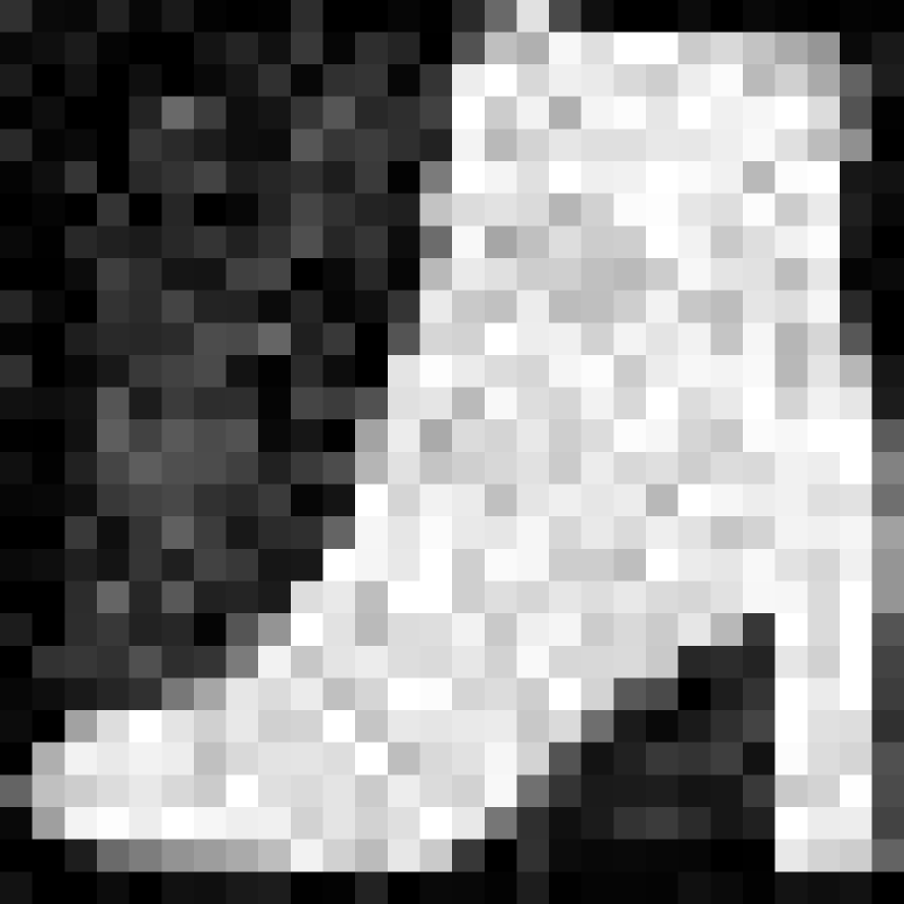
(f)

$\ell_{\infty}$ dist.$=0.394$

pred.=“Bag”

Figure 1: MNIST and Fashion-MNIST examples and their adversarial examples found using the untargeted attack proposed by Cheng et al. (2019) on 200-tree gradient boosted decision tree (GBDT) models trained using XGBoost with depth=8. Natural GBDT models (nat.) are fooled by small $\ell_{\infty}$ perturbations (b, e), while our robust (rob.) GBDT models require much larger perturbations (c, f) for successful attacks. For both MNIST and Fashion-MNIST robust models, we use $\epsilon=0.3$ (a robust training hyper-parameter which will be introduced in Section 4). More examples are shown in the appendix.

In our paper, in addition to Kantchelian attacks we also use a general attack method proposed in Cheng et al. (2019) which does not rely on the gradient nor the smoothness of output of a machine learning model. Cheng’s attack method has been used to efficiently evaluate the robustness of complex models on large datasets, even under black-box settings. To deal with non-smoothness of model output, this method focuses on the distance between the benign example and the decision boundary, and reformulates the adversarial attack as a minimization problem of this distance. Despite the non-smoothness of model prediction, the distance to decision boundary is usually smooth within a local region, and can be found by binary search on vector length given a direction vector. To minimize this distance without gradient, Cheng et al. (2019) used a zeroth order optimization algorithm with a randomized gradient-free method. In our paper, we use the $\ell_{\infty}$ version of Cheng’s attack.

Some adversarial examples obtained by this method are shown in Figure 1, where we display results on both MNIST and Fashion-MNIST datasets. The models we test are natural GBDT models trained using XGBoost and our robust GBDT models, each with 200 trees and a tree depth of 8. Cheng’s attack is able to craft adversarial examples with very small distortions on natural models; for human eyes, the adversarial distortion added to the natural model’s adversarial examples appear as imperceptible noise. We also conduct white-box attacks using the MILP formulation (Kantchelian et al., 2016), which takes much longer time to solve but the $\ell_{\infty}$ distortion found by MILP is comparable to Cheng’s method; see Section 5 for more details. In contrast, for our robust GBDT model, the required adversarial example distortions are so large that we can even vaguely see a number 8 in subfigure (c). The substantial increase in the $\ell_{\infty}$ distortion required to misclassify as well as the increased visual impact of such distortions shows the effectiveness of our robust decision tree training, which we will introduce in detail next. In the main text, we use the $\ell_{\infty}$ version of Kantchelian’s attack; we present results of $\ell_{1}$ and $\ell_{2}$ Kantchelian attacks in the appendix.

4 Robust Decision Trees

4.1 Intuition

As shown in Section 3, tree-based models are vulnerable to adversarial examples. Thus it is necessary to augment the classical natural tree training procedure in order to obtain reliable models robust against adversarial attacks. Our method formulates the process of optimally finding best split threshold in decision tree training as a robust optimization problem. As a conceptual illustration, Figure 2 presents a special case where the traditional greedy optimal splitting may yield non-robust models. A horizontal split achieving high accuracy or score on original points may be easily compromised by adversarial perturbations. On the other hand, we are able to select a better vertical split considering possible perturbations in $\ell_{\infty}$ balls. At a high level, the robust splitting feature and threshold take the distances between data points into account (which is often ignored in most decision tree learning algorithms) and tries to optimize the worst case performance under adversarial perturbations. Some recent works in DNNs (Ilyas et al., 2019; Tsipras et al., 2019) divided features into two categories, robust features and non-robust features. In tree-based models, the effect of this dichotomy on the robustness is straight forward, as seen in the two different splits in Figure 2 using $x^{(1)}$ (a robust feature) and $x^{(2)}$ (a non-robust feature).

Figure 2: (Best viewed in color) A simple example illustrating how robust splitting works. Upper: A set of 10 points that can be easily separated with a horizontal split on feature $x^{(2)}$. The accuracy of this split is 0.8. Middle: The high accuracy horizontal split cannot separate the $\ell_{\infty}$ balls around the data points and thus an adversary can perturb any example $\mathbf{x}_{i}$ within the indicated $\ell_{\infty}$ ball to mislead the model. The worst case accuracy under adversarial perturbations is 0 if all points are perturbed within the square boxes ($\ell_{\infty}$ norm bounded noise). Lower: a more robust split would be a split on feature $x^{(1)}$. The accuracy of this split is 0.7 under all possible perturbations within the same size $\ell_{\infty}$ norm bounded noise (square boxes).

4.2 General Robust Decision Tree Framework

In this section we formally introduce our robust decision tree training framework. For a training set with $N$ examples and $d$ real valued features $\mathcal{D}=\{(\mathbf{x}_{i},y_{i})\}$ ($1\leq i\leq N$, $y_{i}\in\mathbb{R}$, $\mathbf{x}_{i}=[x_{i}^{(1)},x_{i}^{(2)},\dots,x_{i}^{(j)},\dots,x_{i}^{(d)}]\in\mathbb{R}^{d}$), we first normalize the feature values to $[0,\ 1]$ such that $\mathbf{x}_{i}\in[0,1]^{d}$ (the best feature value for split will also be scaled accordingly, but it is irrelevant to model performance). For a general decision tree based learning model, at a given node, we denote $\mathcal{I}\subseteq\mathcal{D}$ as the set of points at that node. For a split on the $j$-th feature with a threshold $\eta$, the sets that will be mentioned in Sections 4.2,  4.3 and 4.4 are summarized in Table 1.

Notation	Definition
$\mathcal{I}$	set of examples on the current node
$\mathcal{I}_{0}$	$\mathcal{I}\cap\{(\mathbf{x}_{i},y_{i})|y_{i}=0\}$ (for classification)
$\mathcal{I}_{1}$	$\mathcal{I}\cap\{(\mathbf{x}_{i},y_{i})|y_{i}=1\}$ (for classification)
$\mathcal{I}_{L}$	$\mathcal{I}\cap\{(\mathbf{x}_{i},y_{i})|x^{(j)}<\eta\}$
$\mathcal{I}_{R}$	$\mathcal{I}\cap\{(\mathbf{x}_{i},y_{i})|x^{(j)}\geq\eta\}$
$\Delta\mathcal{I}$	$\mathcal{I}\cap\{(\mathbf{x}_{i},y_{i})|\eta-\epsilon\leq x^{(j)}\leq\eta+\epsilon$}
$\Delta\mathcal{I}_{L}$	$\Delta\mathcal{I}\cap\mathcal{I}_{L}$
$\Delta\mathcal{I}_{R}$	$\Delta\mathcal{I}\cap\mathcal{I}_{R}$
$\mathcal{I}_{L}^{o}$	$\mathcal{I}_{L}\setminus\Delta\mathcal{I}$
$\mathcal{I}_{R}^{o}$	$\mathcal{I}_{R}\setminus\Delta\mathcal{I}$

Table 1: Notations of different sets in Section 4. We assume a split is made on the $j$-th feature with a threshold $\eta$, and this feature can be perturbed by $\pm\epsilon$.

In classical tree based learning algorithms (which we refer to as “natural” trees in this paper), the quality of a split on a node can be gauged by a score function $S(\cdot)$: a function of the splits on left and right child nodes ($\mathcal{I}_{L}$ and $\mathcal{I}_{R}$), or equivalently on the chosen feature $j$ to split and a corresponding threshold value $\eta$. Since $\mathcal{I}_{L}$ and $\mathcal{I}_{R}$ are determined by $j$, $\eta$ and $\mathcal{I}$, we abuse the notation and define $S(j,\ \eta,\ \mathcal{I}):=S(\mathcal{I}_{L},\ \mathcal{I}_{R})$.

Traditionally, people consider different scores for choosing the “best” split, such as information gain used by ID3 (Quinlan, 1986) and C4.5 (Quinlan, 1986), or Gini impurity in CART (Breiman, 1984). Modern software packages (Chen & Guestrin, 2016; Ke et al., 2017; Dorogush et al., 2018) typically find the best split that minimize a loss function directly, allowing decision trees to be used in a large class of problems (i.e., mean square error loss for regression, logistic loss for classification, and ranking loss for ranking problems). A regular (“natural”) decision tree training process will either exactly or approximately evaluate the score function, for all possible features and split thresholds on the leaf to be split, and select the best $j,\ \eta$ pair:

$$j^{*},\eta^{*}=\operatorname*{arg\,max}_{j,\ \eta}\ S(\mathcal{I}_{L},\ \mathcal{I}_{R})=\operatorname*{arg\,max}_{j,\ \eta}\ S(j,\ \eta,\ \mathcal{I}).$$ (1)

In our setting, we consider the case where features of examples in $\mathcal{I}_{L}$ and $\mathcal{I}_{R}$ can be perturbed by an adversary. Since a typical decision tree can only split on a single feature at one time, it is natural to consider adversarial perturbations within an $\ell_{\infty}$ ball of radius $\epsilon$ around each example $\mathbf{x}_{i}$:

$$\mathit{B}_{\epsilon}^{\infty}(\mathbf{x}_{i})\vcentcolon=[x_{i}^{(1)}-\epsilon,\ x_{i}^{(1)}+\epsilon]\times\dots\times[x_{i}^{(d)}-\epsilon,\ x_{i}^{(d)}+\epsilon].$$

Such perturbations enable the adversary to minimize the score obtained by our split. So instead of finding a split with highest score, an intuitive approach for robust training is to maximize the minimum score value obtained by all possible perturbations in an $\ell_{\infty}$ ball with radius $\epsilon$,

$$j^{*},\ \eta^{*}=\operatorname*{arg\,max}_{j,\ \eta}\ RS(j,\ \eta,\ \mathcal{I}),$$ (2)

where $RS(\cdot)$ is a robust score function defined as

$$\begin{split}&RS(j,\ \eta,\ \mathcal{I})\vcentcolon=\min_{\mathcal{I}^{\prime}=\{(\mathbf{x}^{\prime}_{i},\ y_{i})\}}S(j,\ \eta,\ \mathcal{I}^{\prime})\\ &\text{s.t. }\mathbf{x}^{\prime}_{i}\in\mathit{B}_{\epsilon}^{\infty}(\mathbf{x}_{i})\text{, for all }\mathbf{x}^{\prime}_{i}\in\mathcal{I}^{\prime}.\end{split}$$ (3)

In other words, each $\mathbf{x}_{i}\in\mathcal{I}$ can be perturbed individually under an $\ell_{\infty}$ norm bounded perturbation to form a new set of training examples $\mathcal{I}^{\prime}$. We consider the worst case perturbation, such that the set $\mathcal{I}^{\prime}$ triggers the worst case score after split with feature $j$ and threshold $\eta$. The training objective (2) becomes a max-min optimization problem.

Note that there is an intrinsic consistency between boundaries of the $\ell_{\infty}$ balls and the decision boundary of a decision tree. For the split on the $j$-th feature, perturbations along features other than $j$ do not affect the split. So we only need to consider perturbations within $\pm\epsilon$ along the $j$-th feature. We define $\Delta\mathcal{I}$ as the ambiguity set, containing examples with feature $j$ inside the $[\eta-\epsilon,\eta+\epsilon]$ region (see Table 1). Only examples in $\Delta\mathcal{I}$ may be perturbed from $\mathcal{I}_{L}$ to $\mathcal{I}_{R}$ or from $\mathcal{I}_{R}$ to $\mathcal{I}_{L}$ to reduce the score. Perturbing points in $\mathcal{I}\setminus\Delta\mathcal{I}$ will not change the score or the leaves they are assigned to. We denote $\mathcal{I}_{L}^{o}$ and $\mathcal{I}_{R}^{o}$ as the set of examples that are certainly on the left and right child leaves under perturbations (see Table 1 for definitions). Then we introduce 0-1 variables $s_{i}=\{0,1\}$ denoting an example in the ambiguity set $\Delta\mathcal{I}$ to be assigned to $\mathcal{I}_{L}$ and $\mathcal{I}_{R}$, respectively. Then the $RS$ can be formulated as a 0-1 integer optimization problem with $|\Delta\mathcal{I}|$ variables, which is NP-hard in general. Additionally, we need to scan through all $d$ features of all examples and solve $O(|\mathcal{I}|d)$ minimization problems for a single split at a single node. This large number of problems to solve makes this computation intractable. Therefore, we need to find an approximation for the $RS(j,\ \eta,\ \mathcal{I})$. In Sections 4.3 and 4.4, we present two different approximations and corresponding implementations of our robust decision tree framework, first for classical decision trees with information gain score, and then for modern tree boosting systems which can minimize any loss function.

It is worth mentioning that we normalize features to $[0,\ 1]^{d}$ for the sake of simplicity in this paper. One can also define $\epsilon_{1},\ \epsilon_{2},\ \dots,\ \epsilon_{d}$ for each feature and then the adversary is allowed to perturb $\mathbf{x}_{i}$ within $[x_{i}^{(1)}-\epsilon_{1},\ x_{i}^{(1)}+\epsilon_{1}]\times\dots\times[x_{i}^{(d)}-\epsilon_{d},\ x_{i}^{(d)}+\epsilon_{d}]$. In this case, we would not need to normalize the features. Also, $\epsilon$ is a hyper-parameter in our robust model. Models trained with larger $\epsilon$ are expected to be more robust and when $\epsilon=0$, the robust model is the same as a natural model.

4.3 Robust Splitting for Decision Trees with Information Gain Score

Here we consider a decision tree for binary classification, $y_{i}\in\{0,1\}$, with information gain as the metric for node splitting. The information gain score is

$$S(j,\ \eta,\ \mathcal{I})\vcentcolon=IG(j,\ \eta)=H(y)-H(y|x^{(j)}<\eta),$$

where $H(\cdot)$ and $H(\cdot|\cdot)$ are entropy and conditional entropy on the empirical distribution. For simplicity, we denote $N_{0}\vcentcolon=|\mathcal{I}_{0}|$, $N_{1}\vcentcolon=|\mathcal{I}_{1}|$, $n_{0}\vcentcolon=|\mathcal{I}_{L}\cap\mathcal{I}_{0}|$ and $n_{1}\vcentcolon=|\mathcal{I}_{L}\cap\mathcal{I}_{1}|$. The following theorem shows adversary’s perturbation direction to minimize the information gain.

Theorem 1.

If $\frac{n_{0}}{N_{0}}<\frac{n_{1}}{N_{1}}$ and $\frac{n_{0}+1}{N_{0}}\leq\frac{n_{1}}{N_{1}}$, perturbing one example in $\Delta\mathcal{I}_{R}$ with label 0 to $\mathcal{I}_{L}$ will decrease the information gain.

Similarly, if $\frac{n_{1}}{N_{1}}<\frac{n_{0}}{N_{0}}$ and $\frac{n_{1}+1}{N_{1}}\leq\frac{n_{0}}{N_{0}}$, perturbing one example in $\Delta\mathcal{I}_{R}$ with label 1 to $\mathcal{I}_{L}$ will decrease the information gain. The proof of this theorem will be presented in Section A in the appendix. Note that we also have a similar conclusion for Gini impurity score, which will be shown in Section B in the appendix. Therefore, to decrease the information gain score, the adversary needs to perturb examples in $\Delta\mathcal{I}$ such that $\frac{n_{0}}{N_{0}}$ and $\frac{n_{1}}{N_{1}}$ are close to each other (the ideal case $\frac{n_{0}}{N_{0}}=\frac{n_{1}}{N_{1}}$ may not be achieved because $n_{0}$, $n_{1}$, $N_{0}$ and $N_{1}$ are integers). The robust split finding algorithm is shown in Algorithm 1. In this algorithm we find a perturbation that minimizes $\left|\frac{n_{0}}{N_{0}}-\frac{n_{1}}{N_{1}}\right|$ as an approximation and upper bound to the optimal solution. Algorithm 3 in Section A in the appendix shows an $O(|\mathcal{I}|)$ procedure to find such perturbation to approximately minimize the information gain. Since the algorithm scans through $\{x^{(j)}_{1},\dots,x^{(j)}_{d}\}$ in the sorted order, the sets $\Delta\mathcal{I}$, $\mathcal{I}^{o}_{L},\mathcal{I}^{o}_{R}$ can be maintained in amortized $O(1)$ time in the inner loop. Therefore, the computational complexity of the robust training algorithm is $O(d|\mathcal{I}|^{2})$ per split.

Although it is possible to extend our conclusion to other traditional scores of classification trees, we will focus on the modern scenario where we use a regression tree to fit any loss function in Section 4.4.

Algorithm 1 Robust Split with Information Gain

  Input: Training set $\{(x_{i},\ y_{i})\}|_{i=1}^{N}$, $x_{i}\in[0,1]^{d}$, $y_{i}\in\{0,1\}$.

  Input: The instance set of the current node $I$.

  Input: $\epsilon$, the radius of the $\ell_{\infty}$ ball.

  Output: Optimal split of the current node.

  $\mathcal{I}_{0}\leftarrow\{(x_{i},\ y_{i})|y_{i}=0\},\mathcal{I}_{1}\leftarrow\{(x_{i},\ y_{i})|y_{i}=1\}$;

  $N_{0}\leftarrow|\mathcal{I}\cap\mathcal{I}_{0}|,\ N_{1}\leftarrow|\mathcal{I}\cap\mathcal{I}_{1}|$;

  for $j\leftarrow 1$ to $d$ do

     for $m$ in sorted($\mathcal{I}$, ascending order by $x_{m}^{j}$) do

        $\eta\leftarrow\frac{1}{2}(x_{m}^{j}+x_{m+1}^{j})$, $\Delta\mathcal{I}\leftarrow\mathcal{I}\cap\{(x_{i},\ y_{i})|\eta-\epsilon\leq x^{(j)}\leq\eta+\epsilon\}$;

        $\mathcal{I}_{L}^{o}\leftarrow\{(x_{i},\ y_{i})|x^{(j)}<\eta-\epsilon\},\mathcal{I}_{R}^{o}\leftarrow\{(x_{i},\ y_{i})|x^{(j)}>\eta+\epsilon\}$;

        $n_{0}^{o}\leftarrow|\mathcal{I}_{L}^{o}\cap\mathcal{I}_{0}|$, $n_{1}^{o}\leftarrow|\mathcal{I}_{L}^{o}\cap\mathcal{I}_{1}|$;

        Find $\Delta n_{0}^{*}$, $\Delta n_{1}^{*}$ to minimize $|\frac{\Delta n_{0}^{*}+n_{0}^{o}}{N_{0}}-\frac{\Delta n_{1}^{*}+n_{1}^{o}}{N_{1}}|$ using Algorithm 3 in Section A in the appendix;

        From $\Delta\mathcal{I}$, add $\Delta n_{0}^{*}$ points with $y=0$ and $\Delta n_{1}^{*}$ points with $y=1$ to $\mathcal{I}_{L}^{o}$ and obtain $\mathcal{I}_{L}$;

        Add remaining points in $\Delta\mathcal{I}$ to $\mathcal{I}_{R}^{o}$ and obtain $\mathcal{I}_{R}$;

        $RS(j,\ \eta)\leftarrow IG(\mathcal{I}_{L},\mathcal{I}_{R})$;

     end for

  end for

  $j^{*},\eta^{*}\leftarrow\operatorname*{arg\,max}_{j,\ \eta}RS(j,\ \eta)$;

  Split on feature $j^{*}$ with a threshold $\eta^{*}$;

4.4 Robust Splitting for GBDT models

Algorithm 2 Robust Split for Boosted Tree

  Input: training set $\{(x_{i},\ y_{i})\}|_{i=1}^{N}$, $x_{i}\in[0,1]^{d}$, $y_{i}\in\mathbb{R}$.

  Input: The instance set of the current node $I$.

  Input: $\epsilon$, the radius of the $\ell_{\infty}$ ball.

  Output: Optimal split of the current node.

  for $j\leftarrow 1$ to $d$ do

     for $m$ in sorted($\mathcal{I}$, ascending order by $x_{m}^{j}$) do

        $\eta\leftarrow\frac{1}{2}(x_{m}^{j}+x_{m+1}^{j})$;

        $\mathcal{I}_{L}^{o}\leftarrow\{(x_{i},\ y_{i})|x^{(j)}<\eta-\epsilon\},\Delta\mathcal{I}_{L}\leftarrow\mathcal{I}\cap\{(x_{i},\ y_{i})|\eta-\epsilon\leq x^{(j)}<\eta\}$;

        $\mathcal{I}_{R}^{o}\leftarrow\{(x_{i},\ y_{i})|x^{(j)}>\eta+\epsilon\}$, $\Delta\mathcal{I}_{R}\leftarrow\mathcal{I}\cap\{(x_{i},\ y_{i})|\eta\leq x^{(j)}\leq\eta+\epsilon\}$;

        $S_{1}=S(\mathcal{I}_{L},\mathcal{I}_{R})$,  $S_{2}=S(\mathcal{I}_{L}^{o},\ \mathcal{I}_{R}^{o}\cup\Delta\mathcal{I})$, $S_{3}=S(\mathcal{I}_{L}^{o}\cup\Delta\mathcal{I},\mathcal{I}_{R}^{o})$, $S_{4}=S(\mathcal{I}_{L}^{o}\cup\Delta\mathcal{I}_{R},\mathcal{I}_{R}^{o}\cup\Delta\mathcal{I}_{L})$;

        $RS(j,\ \eta)\leftarrow\min\{S_{1},S_{2},S_{3},S_{4}\};$

     end for

  end for

  $j^{*},\eta^{*}\leftarrow\operatorname*{arg\,max}_{j,\ \eta}RS(j,\ \eta)$;

  Split on feature $j^{*}$ with a threshold $\eta^{*}$;

We now introduce the regression tree training process used in many modern tree boosting packages including XGBoost (Chen & Guestrin, 2016), LightGBM (Ke et al., 2017) and CatBoost (Dorogush et al., 2018). Specifically, we focus on the formulation of gradient boosted decision tree (GBDT), which is one of the most successful ensemble models and has been widely used in industry. GBDT is an additive tree ensemble model $\phi(\cdot)$ combining outputs of $K$ trees

$$\hat{y}_{i}=\phi_{K}(\mathbf{x}_{i})=\sum_{k=1}^{K}f_{k}(\mathbf{x}_{i})$$

where each $f_{k}$ is a decision tree and $\hat{y}_{i}$ is the final output for $\mathbf{x}_{i}$. Here we only focus on regression trees where $\hat{y}_{i}\in\mathbb{R}$. Note that even for a classification problem, the modern treatment in GBDT is to consider the data with logistic loss, and use a regression tree to minimize this loss.

During GBDT training, the trees $f_{k}$ are generated in an additive manner: when we consider the tree $f_{K}$, all previous trees $f_{k},k\in\{1,\cdots,K-1\}$ are kept unchanged. For a general convex loss function $l$ (such as MSE or logistic loss), we desire to minimize the following objective

$$\begin{split}&\mathcal{L}(\phi,\mathcal{D})=\sum_{i=1}^{N}l(y_{i},\hat{y}_{i})+\sum_{k=1}^{K}\Omega(f_{k})\\ &=\sum_{i=1}^{N}l\left(y_{i},\phi_{K-1}(\mathbf{x}_{i})+f_{K}(\mathbf{x}_{i})\right)+\sum_{k=1}^{K-1}\Omega(f_{k})+\Omega(f_{K})\end{split}$$

where $\Omega(f)$ is a regularization term to penalize complex trees; for example, in XGBoost, $\Omega(f)=\gamma T+\frac{1}{2}\lambda\|\mathbf{\omega}\|^{2}$, where $T$ is the number of leaves, $\mathbf{\omega}$ is a vector of all leaf predictions and $\lambda,\ \gamma\geq 0$ are regularization constants. Importantly, when we consider $f_{K}$, $\phi_{K-1}$ is a constant. The impact of $f_{K}(\mathbf{x}_{i})$ on $l(y_{i},\hat{y}_{i})$ can be approximated using a second order Taylor expansion:

$$\begin{split}&l(y_{i},\phi_{K}(\mathbf{x}_{i}))\approx\hat{l}(y_{i},\phi_{K}(\mathbf{x}_{i}))\\ &:=l(y_{i},\phi_{K-1}(\mathbf{x}_{i}))+g_{i}f_{K}(\mathbf{x}_{i})+\frac{1}{2}h_{i}(f_{K}(\mathbf{x}_{i}))^{2}\end{split}$$

where $g_{i}=\frac{\partial l(y_{i},\phi_{K}(\mathbf{x}_{i}))}{\partial f_{K}(\mathbf{x}_{i})}$ and $h_{i}=\frac{\partial^{2}l(y_{i},\phi_{K}(\mathbf{x}_{i}))}{\partial f_{K}^{2}(\mathbf{x}_{i})}$ are the first and second order derivatives on the loss function with respect to the prediction of decision tree $f_{K}$ on point $\mathbf{x}_{i}$. Conceptually, ignoring the regularization terms, the score function can be given as:

$$\begin{split}&S(\mathcal{I}_{L},\mathcal{I}_{R})=\sum_{i\in\mathcal{I}_{L}}\hat{l}(y_{i},\phi_{K}(\mathbf{x}_{i}))\rvert_{\phi_{K}(\mathbf{x}_{i})=\omega_{L}}\\ &+\!\sum_{i\in\mathcal{I}_{R}}\!\hat{l}(y_{i},\phi_{K}(\mathbf{x}_{i}))\rvert_{\phi_{K}(\mathbf{x}_{i})=\omega_{R}}\!-\!\sum_{i\in\mathcal{I}}\!\hat{l}(y_{i},\phi_{K}(\mathbf{x}_{i}))\rvert_{\phi_{K}(\mathbf{x}_{i})=\omega_{P}}\end{split}$$

where $\omega_{L}$, $\omega_{R}$ and $\omega_{P}$ are the prediction values of the left, right and parent nodes. The score represents the improvements on reducing the loss function $\mathcal{L}$ for all data examples in $\mathcal{I}$. The exact form of score used in XGBoost with regularization terms is given in (Chen & Guestrin, 2016):

$$\begin{split}&S(j,\ \eta,\ \mathcal{I})=S(\mathcal{I}_{L},\ \mathcal{I}_{R})\\ &\!:=\!\frac{1}{2}\bigg{[}\frac{(\sum_{i\in\mathcal{I}_{L}}g_{i})^{2}}{\sum_{i\in\mathcal{I}_{L}}h_{i}+\lambda}\!+\!\frac{(\sum_{i\in\mathcal{I}_{R}}g_{i})^{2}}{\sum_{i\in\mathcal{I}_{R}}h_{i}+\lambda}\!-\!\frac{(\sum_{i\in\mathcal{I}}g_{i})^{2}}{\sum_{i\in\mathcal{I}}h_{i}+\lambda}\bigg{]}-\gamma,\end{split}$$

where $\gamma$ is a regularization constant. Again, to minimize the score by perturbing points in $\Delta\mathcal{I}$, the adversary needs to solve an intractable 0-1 integer optimization at each possible splitting position. Since GBDT is often deployed in large scale data mining tasks with a large amount of training data to scan through at each node, and we need to solve $RS$ $O(|\mathcal{I}|d)$ times, we cannot afford any expensive computation. For efficiency, our robust splitting procedure for boosted decision trees, as detailed in Algorithm 2, approximates the minimization by considering only four representative cases: (1) no perturbations: $S_{1}=S(\mathcal{I}_{L},\ \mathcal{I}_{R})$; (2) perturb all points in $\Delta\mathcal{I}$ to the right: $S_{2}=S(\mathcal{I}_{L}^{o},\mathcal{I}_{R}^{o}\cup\Delta\mathcal{I})$; (3) perturb all points in $\Delta\mathcal{I}$ to the left: $S_{3}=S(\mathcal{I}_{L}^{o}\cup\Delta\mathcal{I},\mathcal{I}_{R}^{o})$; (4) swap the points in $\Delta\mathcal{I}$: $S_{4}=S(\mathcal{I}_{L}^{o}\cup\Delta\mathcal{I}_{R},\mathcal{I}_{R}^{o}\cup\Delta\mathcal{I}_{L})$. We take the minimum among the four representative cases as an approximation of the $RS$:

$$RS(j,\ \eta,\ \mathcal{I})\approx\min\{S_{1},\ S_{2},\ S_{3},\ S_{4}\}.$$ (4)

Though this method only takes $O(1)$ time to give a rough approximation of the $RS$ at each possible split position, it is effective empirically as demonstrated next in Section 5.

5 Experiments

Our code is at https://github.com/chenhongge/RobustTrees.

5.1 Robust Information Gain Decision Trees

We present results on three small datasets with robust information gain based decision trees using Algorithm 1. We focus on untargeted adversarial attacks. For each dataset we test on 100 examples (or the whole test set), and we only attack correctly classified images. Attacks proceed until the attack success rate is 100%; the differences in robustness are reflected in the distortion of the adversarial examples required to achieve a successful attack. In Table 2, we present the average $\ell_{\infty}$ distortion of the adversarial examples of both classical natural decision trees and our robust decision trees trained on different datasets. We use Papernot’s attack as well as $\ell_{\infty}$ versions of Cheng’s and Kantchelian’s attacks. The $\ell_{1}$ and $\ell_{2}$ distortion found by Kantchelian’s $\ell_{1}$ and $\ell_{2}$ attacks are presented in Table 4 in the appendix. The adversarial examples found by Cheng’s, Papernot’s and Kantchelian’s attacks have much larger $\ell_{\infty}$ norm for our robust trees compared to those for the natural trees, demonstrating that our robust training algorithm improves the decision tree robustness substantially. In some cases our robust decision trees also have higher test accuracy than the natural trees. This may be due to the fact that the robust score tends to encourage the tree to split at thresholds where fewer examples are in the ambiguity set, and thus the split is also robust against random noise in the training set. Another possible reason is the implicit regularization in the robust splitting. The robust score is always lower than the regular score and thus our splitting is more conservative. Also, from results in Table 2 we see that most of the adversarial examples found by Papernot’s attack have larger $\ell_{\infty}$ norm than those found by Cheng’s $\ell_{\infty}$ attack. This suggests that the straight-forward greedy search attack is not as good as a sophisticated general attack for attacking decision trees. Cheng’s attack is able to achieve similar $\ell_{\infty}$ distortion as Kantchelian’s attack, without solving expensive MILPs. While not scalable to large datasets, Kantchelian’s attack can find the minimum adversarial examples, reflecting the true robustness of a tree-based model.

Dataset	training	test	# of	# of	robust $\epsilon$	depth		test acc.		avg. $\ell_{\infty}$ dist. by Cheng’s $\ell_{\infty}$ attack		avg. $\ell_{\infty}$ dist. by Papernot’s attack		avg. $\ell_{\infty}$ dist. by Kantchelian’s $\ell_{\infty}$ attack
	set size	set size	features	classes		robust	natural	robust	natural	robust	natural	robust	natural	robust	natural
breast-cancer	546	137	10	2	0.3	5	5	.948	.942	.531	.189	.501	.368	.463	.173
diabetes	614	154	8	2	0.2	5	5	.688	.747	.206	.065	.397	.206	.203	.060
ionosphere	281	70	34	2	0.2	4	4	.986	.929	.388	.109	.408	.113	.358	.096

Table 2: Test accuracy and robustness of information gain based single decision tree model. The robustness is evaluated by the average $\ell_{\infty}$ distortion of adversarial examples found by Cheng’s, Papernot’s and Kantchelian’s attacks. Average $\ell_{\infty}$ distortion of robust decision tree models found by three attack methods are consistently larger than that of the naturally trained ones.

5.2 Robust GBDT Models

In this subsection, we evaluate our algorithm in the tree boosting setting, where multiple robust decision trees are created in an ensemble to improve model accuracy. We implement Algorithm 2 by slightly modifying the node splitting procedure in XGBoost. Our modification is only relevant to computing the scores for selecting the best split, and is compatible with other existing features of XGBoost. We also use XGBoost to train natural (undefended) GBDT models. Again, we focus on untargeted adversarial attacks. We consider nine real world large or medium sized datasets and two small datasets (Chang & Lin, 2011), spanning a variety of data types (including both tabular and image data). For small datasets we use 100 examples and for large or medium sized datasets, we use 5000 examples for robustness evaluation, except for MNIST 2 vs. 6, where we use 100 examples. MNIST 2 vs. 6 is a subset of MNIST to only distinguish between 2 and 6. This is the dataset tested in Kantchelian et al. (2016). We use the same number of trees, depth and step size shrinkage as in Kantchelian et al. (2016) to train our robust and natural models. Same as Kantchelian et al. (2016), we only test 100 examples for MNIST 2 vs. 6 since the model is relatively large. In Table 3, we present the average $\ell_{\infty}$ distortion of adversarial examples found by Cheng’s $\ell_{\infty}$ attack for both natural GBDT and robust GBDT models trained on those datasets. For small and medium binary classification models, we also present results of Kantchelian’s $\ell_{\infty}$ attack, which finds the minimum adversarial example in $\ell_{\infty}$ norm. The $\ell_{1}$ and $\ell_{2}$ distortion found by Kantchelian’s $\ell_{1}$ and $\ell_{2}$ attacks are presented in Table 5 in the appendix. Kantchelian’s attack can only handle binary classification problems and small scale models due to its time-consuming MILP formulation. Papernot’s attack is inapplicable here because it is for attacking a single tree only. The natural and robust models have the same number of trees for comparison. We only attack correctly classified images and all examples are successfully attacked. We see that our robust GBDT models consistently outperform the natural GBDT models in terms of $\ell_{\infty}$ robustness.

For some datasets, we need to increase tree depth in robust GBDT models in order to obtain accuracy comparable to the natural GBDT models. The requirement of larger model capacity is common in the adversarial training literature: in the state-of-the-art defense for DNNs, Madry et al. (2018) argues that increasing the model capacity is essential for adversarial training to obtain good accuracy.

Dataset	training	test	# of	# of	# of	robust	depth		test acc.		avg. $\ell_{\infty}$ dist. by Cheng’s $\ell_{\infty}$ attack		dist.	avg. $\ell_{\infty}$ dist. by Kantchelian’s $\ell_{\infty}$ attack		dist.
	set size	set size	features	classes	trees	$\epsilon$	robust	natural	robust	natural	robust	natural	improv.	robust	natural	improv.
breast-cancer	546	137	10	2	4	0.3	8	6	.978	.964	.411	.215	1.91X	.406	.201	2.02X
covtype	400,000	181,000	54	7	80	0.2	8	8	.847	.877	.081	.061	1.31X	not binary	not binary	—
cod-rna	59,535	271,617	8	2	80	0.2	5	4	.880	.965	.062	.053	1.16X	.054	.034	1.59X
diabetes	614	154	8	2	20	0.2	5	5	.786	.773	.139	.060	2.32X	.114	.047	2.42X
Fashion-MNIST	60,000	10,000	784	10	200	0.1	8	8	.903	.903	.156	.049	3.18X	not binary	not binary	—
HIGGS	10,500,000	500,000	28	2	300	0.05	8	8	.709	.760	.022	.014	1.57X	time out	time out	—
ijcnn1	49,990	91,701	22	2	60	0.1	8	8	.959	.980	.054	.047	1.15X	.037	.031	1.19X
MNIST	60,000	10,000	784	10	200	0.3	8	8	.980	.980	.373	.072	5.18X	not binary	not binary	—
Sensorless	48,509	10,000	48	11	30	0.05	6	6	.987	.997	.035	.023	1.52X	not binary	not binary	—
webspam	300,000	50,000	254	2	100	0.05	8	8	.983	.992	.049	.024	2.04X	time out	time out	—
MNIST 2 vs. 6	11,876	1,990	784	2	1000	0.3	6	4	.997	.998	.406	.168	2.42X	.315	.064	4.92X

Table 3: The test accuracy and robustness of GBDT models. Average $\ell_{\infty}$ distortion of our robust GBDT models are consistently larger than those of the naturally trained models. The robustness is evaluated by the average $\ell_{\infty}$ distortion of adversarial examples found by Cheng’s and Kantchelian’s attacks. Only small or medium sized binary classification models can be evaluated by Kantchelian’s attack, but it finds the minimum adversarial example with smallest possible distortion.

Figure 3 and Figure 5 in the appendix show the distortion and accuracy of MNIST and Fashion-MNIST models with different number of trees. The adversarial examples are found by Cheng’s $\ell_{\infty}$ attack. Models with $k$ trees are the first $k$ trees during a single boosting run of $K$ ($K\geq k$) trees. The $\ell_{\infty}$ distortion of robust models are consistently much larger than those of the natural models. For MNIST dataset, our robust GBDT model loses accuracy slightly when the model has only 20 trees. This loss is gradually compensated as more trees are added to the model; regardless of the number of trees in the model, the robustness improvement is consistently observed, as our robust training is embedded in each tree’s building process and we create robust trees beginning from the very first step of boosting. Adversarial training in Kantchelian et al. (2016), in contrast, adds adversarial examples with respect to the current model at each boosting round so adversarial examples produced in the later stages of boosting are only learned by part of the model. The non-robust trees in the first few rounds of boosting still exist in the final model and they may be the weakness of the ensemble. Similar problems are not present in DNN adversarial training since the whole model is exposed to new adversarial examples throughout the training process. This may explain why adversarial training in Kantchelian et al. (2016) failed to improve $\ell_{1}$, $\ell_{2}$, or $\ell_{\infty}$ robustness on the MNIST 2 vs. 6 model, while our method achieves significant robustness improvement with the same training parameters and evaluation metrics, as shown in Tables 3 and 5. Additionally, we also evaluate the robustness of natural and robust models with different number of trees on a variety of datasets using Cheng’s $\ell_{\infty}$ attack, presented in Table 7 in the appendix.

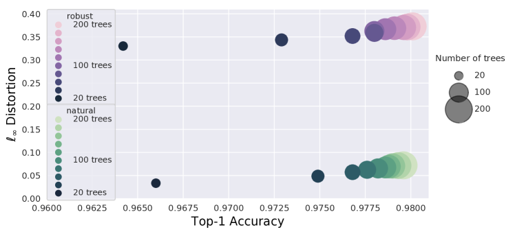
Figure 3: (Best viewed in color) $\ell_{\infty}$ distortion vs. classification accuracy of GBDT models on MNIST dataset with different numbers of trees (circle size). The adversarial examples are found by Cheng’s $\ell_{\infty}$ attack. The robust training parameter $\epsilon=0.3$ for MNIST. With robust training (purple) the distortion needed to fool a model increases dramatically with less than $1\%$ accuracy loss.

We also test our framework on random forest models and the results are shown in Section G in the appendix.

6 Conclusion

In this paper, we study the robustness of tree-based machine learning models under adversarial attacks. Our experiments show that just as in DNNs, tree-based models are also vulnerable to adversarial attacks. To address this issue, we propose a novel robust decision tree training framework. We make necessary approximations to ensure scalability and implement our framework in both classical decision tree and tree boosting settings. Extensive experiments on a variety of datasets show that our method substantially improves model robustness. Our framework can be extended to other tree-based models such as Gini impurity based classification trees, random forest, and CART.

Appendix A Proof of Theorem 1

Here we prove Theorem 1 for information gain score.

Proof.

$H(y)$ and $H(y|x^{(j)}<\eta)$ are defined as

$$H(y)=-\frac{|\mathcal{I}_{0}|}{|\mathcal{I}|}\log(\frac{|\mathcal{I}_{0}|}{|\mathcal{I}|})-\frac{|\mathcal{I}_{1}|}{|\mathcal{I}|}\log(\frac{|\mathcal{I}_{1}|}{|\mathcal{I}|}),$$

and

$$\begin{split}&H(y|x^{(j)}<\eta)=\\ &-\frac{|\mathcal{I}_{L}|}{|\mathcal{I}|}\bigg{[}\frac{|\mathcal{I}_{L}\cap\mathcal{I}_{0}|}{|\mathcal{I}_{L}|}\log(\frac{|\mathcal{I}_{L}\cap\mathcal{I}_{0}|}{|\mathcal{I}_{L}|})+\frac{|\mathcal{I}_{L}\cap\mathcal{I}_{1}|}{|\mathcal{I}_{L}|}\log(\frac{|\mathcal{I}_{L}\cap\mathcal{I}_{1}|}{|\mathcal{I}_{L}|})\bigg{]}\\ &-\frac{|\mathcal{I}_{R}|}{|\mathcal{I}|}\bigg{[}\frac{|\mathcal{I}_{R}\cap\mathcal{I}_{0}|}{|\mathcal{I}_{R}|}\log(\frac{|\mathcal{I}_{R}\cap\mathcal{I}_{0}|}{|\mathcal{I}_{R}|})+\frac{|\mathcal{I}_{R}\cap\mathcal{I}_{1}|}{|\mathcal{I}_{R}|}\log(\frac{|\mathcal{I}_{R}\cap\mathcal{I}_{1}|}{|\mathcal{I}_{R}|})\bigg{]}.\end{split}$$

For simplicity, we denote $N_{0}\vcentcolon=|\mathcal{I}_{0}|$, $N_{1}\vcentcolon=|\mathcal{I}_{1}|$, $n_{0}\vcentcolon=|\mathcal{I}_{L}\cap\mathcal{I}_{0}|$ and $n_{1}\vcentcolon=|\mathcal{I}_{L}\cap\mathcal{I}_{1}|$. The information gain of this split can be written as a function of $n_{0}$ and $n_{1}$:

$$\begin{split}IG&=C_{1}[n_{0}\log(\frac{n_{0}}{N_{0}(n_{1}+n_{0})})+n_{1}\log(\frac{n_{1}}{N_{1}(n_{1}+n_{0})})\\ &+(N_{0}-n_{0})\log(\frac{N_{0}-n_{0}}{N_{0}(N_{1}+N_{0}-n_{1}-n_{0})})\\ &+(N_{1}-n_{1})\log(\frac{N_{1}-n_{1}}{N_{1}(N_{1}+N_{0}-n_{1}-n_{0})})]+C_{2},\end{split}$$ (5)

where $C_{1}>0$ and $C_{2}$ are constants with respect to $n_{0}$. Taking $n_{0}$ as a continuous variable, we have

$$\frac{\partial IG}{\partial n_{0}}=C_{1}\cdot\log(1+\frac{n_{0}N_{1}-N_{0}n_{1}}{(N_{0}-n_{0})(n_{1}+n_{0})})$$ (6)

When $\frac{\partial IG}{\partial n_{0}}<0$, perturbing one example in $\Delta\mathcal{I}_{R}$ with label 0 to $\mathcal{I}_{L}$ will increase $n_{0}$ and decrease the information gain. It is easy to see that $\frac{\partial IG}{\partial n_{0}}<0$ if and only if $\frac{n_{0}}{N_{0}}<\frac{n_{1}}{N_{1}}.$ This indicates that when $\frac{n_{0}}{N_{0}}<\frac{n_{1}}{N_{1}}$ and $\frac{n_{0}+1}{N_{0}}\leq\frac{n_{1}}{N_{1}}$, perturbing one example with label 0 to $\mathcal{I}_{L}$ will always decrease the information gain. ∎

Similarly, if $\frac{n_{1}}{N_{1}}<\frac{n_{0}}{N_{0}}$ and $\frac{n_{1}+1}{N_{1}}\leq\frac{n_{0}}{N_{0}}$, perturbing one example in $\Delta\mathcal{I}_{R}$ with label 1 to $\mathcal{I}_{L}$ will decrease the information gain. As mentioned in the main text, to decrease the information gain score in Algorithm 1, the adversary needs to perturb examples in $\Delta\mathcal{I}$ such that $\frac{n_{0}}{N_{0}}$ and $\frac{n_{1}}{N_{1}}$ are close to each other. Algorithm 3 gives an $O(|\Delta\mathcal{I}|)$ method to find $\Delta n_{0}^{*}$ and $\Delta n_{1}^{*}$, the optimal number of points in $\Delta\mathcal{I}$ with label 0 and 1 to be added to the left.

Algorithm 3 Finding $\Delta n_{0}^{*}$ and $\Delta n_{1}^{*}$ to Minimize Information Gain or Gini Impurity

  Input: $N_{0}$ and $N_{1}$, number of instances with label 0 and 1. $n_{0}^{o}$ and $n_{1}^{o}$, number of instances with label 0 and 1 that are certainly on the left.

  Input: $|\Delta\mathcal{I}\cap\mathcal{I}_{0}|$ and $|\Delta\mathcal{I}\cap\mathcal{I}_{1}|$, number of instances with label 0 and 1 that can be perturbed.

  Output: $\Delta n_{0}^{*}$, $\Delta n_{1}^{*}$, optimal number of points with label 0 and 1 in $\Delta\mathcal{I}$ to be place on the left.

  $\Delta n_{0}^{*}\leftarrow 0,\ \Delta n_{1}^{*}\leftarrow 0,\ \text{min\textunderscore diff}\leftarrow|\frac{n_{0}^{o}}{N_{0}}-\frac{n_{1}^{o}}{N_{1}}|$;

  for $\Delta n_{0}\leftarrow 0$ to $|\Delta\mathcal{I}\cap\mathcal{I}_{0}|$ do

     $\text{ceil}\leftarrow\lceil\frac{N_{1}(n_{0}^{o}+\Delta n_{0})}{N_{0}}\rceil-n_{1}^{o}$;

     $\text{floor}\leftarrow\lfloor\frac{N_{1}(n_{0}^{o}+\Delta n_{0})}{N_{0}}\rfloor-n_{1}^{o}$;

     for $\Delta n^{\prime}_{1}$ in $\{\text{ceil},\ \text{floor}\}$ do

        $\Delta n_{1}\leftarrow\max\{\min\{\Delta n^{\prime}_{1},\ |\Delta\mathcal{I}\cap\mathcal{I}_{1}|\},\ 0\};$

        if $\text{min\textunderscore diff}>|\frac{\Delta n_{0}+n_{0}^{0}}{N_{0}}-\frac{\Delta n_{1}+n_{1}^{0}}{N_{1}}|$ then

           $\Delta n_{0}^{*}\leftarrow\Delta n_{0},\ \Delta n_{1}^{*}\leftarrow\Delta n_{1},\ \text{min\textunderscore diff}\leftarrow|\frac{\Delta n_{0}+n_{0}^{0}}{N_{0}}-\frac{\Delta n_{1}+n_{1}^{0}}{N_{1}}|$;

        end if

     end for

  end for

  Return $\Delta n_{0}^{*}$ and $\Delta n_{1}^{*}$;

Appendix B Gini Impurity Score

We also have a theorem for Gini impurity score similar to Theorem 1.

Theorem 1.

If $\frac{n_{0}}{N_{0}}<\frac{n_{1}}{N_{1}}$ and $\frac{n_{0}+1}{N_{0}}\leq\frac{n_{1}}{N_{1}}$, perturbing one example in $\Delta\mathcal{I}_{R}$ with label 0 to $\mathcal{I}_{L}$ will decrease the Gini impurity.

Proof.

The Gini impurity score of a split with threshold $\eta$ on feature $j$ is

$$\begin{split}Gini&=(1-\frac{|\mathcal{I}_{0}|^{2}}{|\mathcal{I}|^{2}}-\frac{|\mathcal{I}_{1}|^{2}}{|\mathcal{I}|^{2}})\\ &-\frac{|\mathcal{I}_{L}|}{|\mathcal{I}|}(1-\frac{|\mathcal{I}_{0}\cap\mathcal{I}_{L}|^{2}}{|\mathcal{I}_{L}|^{2}}-\frac{|\mathcal{I}_{1}\cap\mathcal{I}_{L}|^{2}}{|\mathcal{I}_{L}|^{2}})\\ &-\frac{|\mathcal{I}_{R}|}{|\mathcal{I}|}(1-\frac{|\mathcal{I}_{0}\cap\mathcal{I}_{R}|^{2}}{|\mathcal{I}_{R}|^{2}}-\frac{|\mathcal{I}_{1}\cap\mathcal{I}_{R}|^{2}}{|\mathcal{I}_{R}|^{2}})\\ &=C_{3}[\frac{n_{0}^{2}+n_{1}^{2}}{n_{1}+n_{0}}+\frac{(N_{0}-n_{0})^{2}+(N_{1}-n_{1})^{2}}{(N_{0}+N_{1}-n_{0}-n_{1})}]+C_{4},\end{split}$$ (7)

where we use the same notation as in (5). $C_{3}>0$ and $C_{4}$ are constants with respect to $n_{0}$. Taking $n_{0}$ as a continuous variable, we have

$$\begin{split}\frac{\partial\ Gini}{\partial n_{0}}=2C_{3}\frac{m_{1}m_{0}(n_{0}m_{1}+n_{1}m_{0}+2n_{1}m_{1})}{(n_{0}+n_{1})^{2}(m_{0}+m_{1})^{2}}(\frac{n_{0}}{m_{0}}-\frac{n_{1}}{m_{1}}),\end{split}$$ (8)

where $m_{0}:=N_{0}-n_{0}$ and $m_{1}:=N_{1}-n_{1}$. Then $\frac{\partial\ Gini}{\partial n_{0}}<0$ holds if $\frac{n_{0}}{m_{0}}<\frac{n_{1}}{m_{1}}$, which is equivalent to $\frac{n_{0}}{N_{0}}<\frac{n_{1}}{N_{1}}.$ ∎

Since the conditions of Theorem 1 and Theorem 1 are the same, Algorithm 1 and Algorithm 3 also work for tree-based models using Gini impurity score.

Appendix C Decision Boundaries of Robust and Natural Models

Figure 4 shows the decision boundaries and test accuracy of natural trees as well as robust trees with different $\epsilon$ values on two dimensional synthetic datasets. All trees have depth 5 and we plot training examples in the figure. The results show that the decision boundaries of our robust decision trees are simpler than the decision boundaries in natural decision trees, agreeing with the regularization argument in the main text.

Figure 4: (Best viewed in color) The decision boundaries and test accuracy of natural decision trees and robust decision trees with depth 5 on synthetic datasets with two features.

Appendix D Omitted Results on $\ell_{1}$ and $\ell_{2}$ distortion

In Tables 4 and 5 we present the $\ell_{1}$ and $\ell_{2}$ distortions of vanilla (information gain based) decision trees and GBDT models obtained by Kantchelian’s $\ell_{1}$ and $\ell_{2}$ attacks. Again, only small or medium sized binary classification models can be evaluated by Kantchelian’s attack. From the results we can see that although our robust decision tree training algorithm is designed for $\ell_{\infty}$ perturbations, it can also improve models $\ell_{1}$ and $\ell_{2}$ robustness significantly.

Appendix E Omitted Results on Models with Different Number of Trees

Figure 5 shows the $\ell_{\infty}$ distortion and accuracy of Fashion-MNIST GBDT models with different number of trees. In Table 7 we present the test accuracy and $\ell_{\infty}$ distortion of models with different number of trees obtained by Cheng’s $\ell_{\infty}$ attack. For each dataset, models are generated during a single boosting run. We can see that the robustness of robustly trained models consistently outperforms that of natural models with the same number of trees. Another interesting finding is that for MNIST and Fashion-MNIST datasets in Figures 3 (in the main text) and 5, models with more trees are generally more robust. This may not be true in other datasets; for example, results from Table 7 in the Appendix shows that on some other datasets, the natural GBDT models lose robustness when more trees are added.

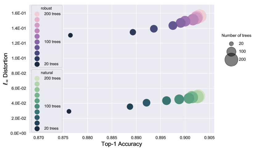
Figure 5: (Best viewed in color) $\ell_{\infty}$ distortion vs. classification accuracy of GBDT models on Fashion-MNIST datasets with different numbers of trees (circle size). The adversarial examples are found by Cheng’s $\ell_{\infty}$ attack. The robust training parameter $\epsilon=0.1$ for Fashion-MNIST. With robust training (purple) the distortion needed to fool a model increases dramatically with less than $1\%$ accuracy loss.

Appendix F Reducing Depth Does Not Improve Robustness

One might hope that one can simply reduce the depth of trees to improve robustness since shallower trees provide stronger regularization effects. Unfortunately, this is not true. As demonstrated in Figure 6, the robustness of naturally trained GBDT models are much worse when compared to robust models, no matter how shallow they are or how many trees are in the ensemble. Also, when the number of trees in the ensemble model is limited, reducing tree depth will significantly lower the model accuracy.

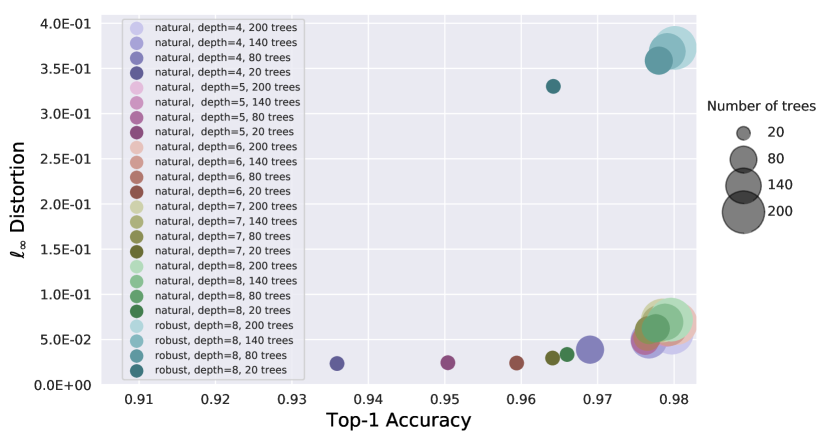
Figure 6: (Best viewed in color) Robustness vs. classification accuracy plot of GBDT models on MNIST dataset with different depth and different numbers of trees. The adversarial examples are found by Cheng’s $\ell_{\infty}$ attack. The robust training parameter $\epsilon=0.3$. Reducing the model depth cannot improve robustness effectively compared to our proposed robust training procedure.

Appendix G Random Forest Model Results

We test our robust training framework on random forest (RF) models and our results are in Table 6. In these experiments we build random forest models with 0.5 data sampling rate and 0.5 feature sampling rate. We test the robust and natural random forest model on three datasets and in each dataset, we tested 100 points using Cheng’s and Kantchelian’s $\ell_{\infty}$ attacks. From the results we can see that our robust decision tree training framework can also significantly improve random forest model robustness.

Appendix H More MNIST and Fashion-MNIST Adversarial Examples

In Figure 7 we present more adversarial examples for MNIST and Fashion-MNIST datasets using GBDT models.

Dataset	training	test	# of	# of	robust $\epsilon$	depth		test acc.		avg. $\ell_{1}$ dist. by Kantchelian’s $\ell_{1}$ attack		avg. $\ell_{2}$ dist. by Kantchelian’s $\ell_{2}$ attack
	set size	set size	features	classes		robust	natural	robust	natural	robust	natural	robust	natural
breast-cancer	546	137	10	2	0.3	5	5	.948	.942	.534	.270	.504	.209
diabetes	614	154	8	2	0.2	5	5	.688	.747	.204	.075	.204	.065
ionosphere	281	70	34	2	0.2	4	4	.986	.929	.358	.127	.358	.106

Table 4: The test accuracy and robustness of information gain based single decision tree models. The robustness is evaluated by the average $\ell_{1}$ and $\ell_{2}$ distortions of adversarial examples found by Kantchelian’s $\ell_{1}$ and $\ell_{2}$ attacks. Average $\ell_{\infty}$ distortions of robust decision tree models found by the two attack methods are consistently larger than those of the naturally trained ones.

Dataset	training	test	# of	# of	# of	robust	depth		test acc.		avg. $\ell_{1}$ dist. by Kantchelian’s $\ell_{1}$ attack		dist.	avg. $\ell_{2}$ dist. by Kantchelian’s $\ell_{2}$ attack		dist.
	set size	set size	features	classes	trees	$\epsilon$	robust	natural	robust	natural	robust	natural	improv.	robust	natural	improv.
breast-cancer	546	137	10	2	4	0.3	8	6	.978	.964	.488	.328	1.49X	.431	.251	1.72X
cod-rna	59,535	271,617	8	2	80	0.2	5	4	.880	.965	.065	.059	1.10X	.062	.047	1.32X
diabetes	614	154	8	2	20	0.2	5	5	.786	.773	.150	.081	1.85X	.135	.059	2.29X
ijcnn1	49,990	91,701	22	2	60	0.1	8	8	.959	.980	.057	.051	1.12X	.048	.042	1.14X
MNIST 2 vs. 6	11,876	1,990	784	2	1000	0.3	6	4	.997	.998	1.843	.721	2.56X	.781	.182	4.29X

Table 5: The test accuracy and robustness of GBDT models. Average $\ell_{1}$ and $\ell_{2}$ distortions of robust GBDT models are consistently larger than those of the naturally trained models. The robustness is evaluated by the average $\ell_{1}$ and $\ell_{2}$ distortions of adversarial examples found by Kantchelian’s $\ell_{1}$ and $\ell_{2}$ attacks.

Dataset	training	test	# of	# of	# of	robust	depth		test acc.		avg. $\ell_{\infty}$ dist. by Cheng’s $\ell_{\infty}$ attack		dist.	avg. $\ell_{\infty}$ dist. by Kantchelian’s $\ell_{\infty}$ attack		dist.
	set size	set size	features	classes	trees	$\epsilon$	robust	natural	robust	natural	robust	natural	improv.	robust	natural	improv.
breast-cancer	546	137	10	2	60	0.3	8	6	.993	.993	.406	.297	1.37X	.396	.244	1.62X
diabetes	614	154	8	2	60	0.2	5	5	.753	.760	.185	.093	1.99X	.154	.072	2.14X
MNIST 2 vs. 6	11,876	1,990	784	2	1000	0.3	6	4	.986	.983	.445	.180	2.47X	.341	.121	2.82X

Table 6: The test accuracy and robustness of random forest models. Average $\ell_{\infty}$ distortion of our robust random forest models are consistently larger than those of the naturally trained models. The robustness is evaluated by the average $\ell_{\infty}$ distortion of adversarial examples found by Cheng’s and Kantchelian’s attacks.

breast-cancer (2) $\epsilon=0.3$ $\text{depth}_{r}=8,\ \text{depth}_{n}=6$	train	test	feat.	# of trees	1		2		3		4		5		6		7		8		9		10
				model	rob.	nat.	rob.	nat.	rob.	nat.	rob.	nat.	rob.	nat.	rob.	nat.	rob.	nat.	rob.	nat.	rob.	nat.	rob.	nat.
	546	137	10	tst. acc.	.985	.942	.971	.964	.978	.956	.978	.964	.985	.964	.985	.964	.985	.971	.993	.971	.993	.971	1.00	.971
				$\ell_{\infty}$ dist.	.383	.215	.396	.229	.411	.216	.411	.215	.406	.226	.407	.229	.406	.248	.439	.234	.439	.238	.437	.241
covtype (7) $\epsilon=0.2$ $\text{depth}_{r}=\text{depth}_{n}=8$	train	test	feat.	# of trees	20		40		60		80		100		120		140		160		180		200
				model	rob.	nat.	rob.	nat.	rob.	nat.	rob.	nat.	rob.	nat.	rob.	nat.	rob.	nat.	rob.	nat.	rob.	nat.	rob.	nat.
	400,000	181,000	54	tst. acc.	.775	.828	.809	.850	.832	.865	.847	.877	.858	.891	.867	.902	.875	.912	.882	.921	.889	.926	.894	.930
				$\ell_{\infty}$ dist.	.125	.066	.103	.064	.087	.062	.081	.061	.079	.060	.077	.059	.077	.058	.075	.056	.075	.056	.073	.055
cod-rna (2) $\epsilon=0.2$ $\text{depth}_{r}=5,\ \text{depth}_{n}=4$	train	test	feat.	# of trees	20		40		60		80		100		120		140		160		180		200
				model	rob.	nat.	rob.	nat.	rob.	nat.	rob.	nat.	rob.	nat.	rob.	nat.	rob.	nat.	rob.	nat.	rob.	nat.	rob.	nat.
	59,535	271,617	8	tst. acc.	.810	.947	.861	.959	.874	.963	.880	.965	.892	.966	.900	.967	.903	.967	.915	.967	.922	.967	.925	.968
				$\ell_{\infty}$ dist.	.077	.057	.066	.055	.063	.054	.062	.053	.059	.053	.057	.052	.056	.052	.056	.052	.056	.052	.058	.052
diabetes (2) $\epsilon=0.2$ $\text{depth}_{r}=\text{depth}_{n}=5$	train	test	feat.	# of trees	2		4		6		8		10		12		14		16		18		20
				model	rob.	nat.	rob.	nat.	rob.	nat.	rob.	nat.	rob.	nat.	rob.	nat.	rob.	nat.	rob.	nat.	rob.	nat.	rob.	nat.
	614	154	8	tst. acc.	.760	.753	.760	.753	.766	.753	.773	.753	.773	.734	.779	.727	.779	.747	.779	.760	.779	.773	.786	.773
				$\ell_{\infty}$ dist.	.163	.066	.163	.065	.154	.071	.151	.071	.152	.073	.148	.072	.146	.067	.144	.062	.138	.062	.139	.060
Fashion-MNIST (10) $\epsilon=0.1$ $\text{depth}_{r}=\text{depth}_{n}=8$	train	test	feat.	# of trees	20		40		60		80		100		120		140		160		180		200
				model	rob.	nat.	rob.	nat.	rob.	nat.	rob.	nat.	rob.	nat.	rob.	nat.	rob.	nat.	rob.	nat.	rob.	nat.	rob.	nat.
	60,000	10,000	784	tst. acc.	.877	.876	.889	.889	.894	.892	.898	.896	.899	.899	.900	.901	.902	.902	.902	.901	.902	.903	.903	.903
				$\ell_{\infty}$ dist.	.131	.029	.135	.035	.139	.041	.144	.043	.147	.045	.149	.047	.151	.048	.153	.048	.154	.049	.156	.049
HIGGS (2) $\epsilon=0.05$ $\text{depth}_{r}=\text{depth}_{n}=8$	train	test	feat.	# of trees	50		100		150		200		250		300		350		400		450		500
				model	rob.	nat.	rob.	nat.	rob.	nat.	rob.	nat.	rob.	nat.	rob.	nat.	rob.	nat.	rob.	nat.	rob.	nat.	rob.	nat.
	10,500,000	500,000	28	tst. acc.	.676	.747	.688	.753	.700	.755	.702	.758	.705	.759	.709	.760	.711	.762	.712	.764	.716	.763	.718	.764
				$\ell_{\infty}$ dist.	.023	.013	.023	.014	.022	.014	.022	.014	.022	.014	.022	.014	.021	.015	.021	.015	.021	.015	.021	.015
ijcnn1 (2) $\epsilon=0.1$ $\text{depth}_{r}=\text{depth}_{n}=8$	train	test	feat.	# of trees	10		20		30		40		50		60		70		80		90		100
				model	rob.	nat.	rob.	nat.	rob.	nat.	rob.	nat.	rob.	nat.	rob.	nat.	rob.	nat.	rob.	nat.	rob.	nat.	rob.	nat.
	49,990	91,701	22	tst. acc.	.933	.973	.942	.977	.947	.977	.952	.979	.958	.980	.959	.980	.962	.980	.964	.980	.967	.980	.968	.980
				$\ell_{\infty}$ dist.	.065	.048	.061	.047	.058	.048	.057	.047	.054	.048	.054	.047	.054	.047	.053	.047	.052	.047	.052	.047
MNIST (10) $\epsilon=0.3$ $\text{depth}_{r}=\text{depth}_{n}=8$	train	test	feat.	# of trees	20		40		60		80		100		120		140		160		180		200
				model	rob.	nat.	rob.	nat.	rob.	nat.	rob.	nat.	rob.	nat.	rob.	nat.	rob.	nat.	rob.	nat.	rob.	nat.	rob.	nat.
	$60,000$	$10,000$	784	tst. acc.	.964	.966	.973	.975	.977	.977	.978	.978	.978	.978	.979	.979	.979	.979	.980	.979	.980	.979	.980	.980
				$\ell_{\infty}$ dist.	.330	.033	.343	.049	.352	.057	.359	.062	.363	.065	.367	.067	.369	.069	.370	.071	.371	.072	.373	.072
Sensorless (11) $\epsilon=0.05$ $\text{depth}_{r}=\text{depth}_{n}=6$	train	test	feat.	# of trees	3		6		9		12		15		18		21		24		27		30
				model	rob.	nat.	rob.	nat.	rob.	nat.	rob.	nat.	rob.	nat.	rob.	nat.	rob.	nat.	rob.	nat.	rob.	nat.	rob.	nat.
	48,509	10,000	48	tst. acc.	.834	.977	.867	.983	.902	.987	.923	.991	.945	.992	.958	.994	.966	.996	.971	.996	.974	.997	.978	.997
				$\ell_{\infty}$ dist.	.037	.022	.036	.022	.035	.023	.035	.023	.035	.023	.035	.023	.035	.023	.035	.023	.035	.023	.035	.023
webspam (2) $\epsilon=0.05$ $\text{depth}_{r}=\text{depth}_{n}=8$	train	test	feat.	# of trees	10		20		30		40		50		60		70		80		90		100
				model	rob.	nat.	rob.	nat.	rob.	nat.	rob.	nat.	rob.	nat.	rob.	nat.	rob.	nat.	rob.	nat.	rob.	nat.	rob.	nat.
	$300,000$	$50,000$	254	tst. acc.	.950	.976	.964	.983	.970	.986	.973	.989	.976	.990	.978	.990	.980	.991	.981	.991	.982	.992	.983	.992
				$\ell_{\infty}$ dist.	.049	.010	.048	.015	.049	.019	.049	.021	.049	.023	.049	.024	.049	.024	.049	.024	.048	.024	.049	.024

Table 7: The test accuracy and robustness of GBDT models. Here $\text{depth}_{n}$ is the depth of natural trees and $\text{depth}_{r}$ is the depth of robust trees. Robustness is evaluated by the average $\ell_{\infty}$ distortion of adversarial examples found by Cheng’s attack (Cheng et al., 2019). The number in the parentheses after each dataset name is the number of classes. Models are generated during a single boosting run. We can see that the robustness of our robust models consistently outperforms that of natural models with the same number of trees.

Original	Adversarial of nat. GBDT	Adversarial of rob. GBDT	Original	Adversarial of nat. GBDT	Adversarial of rob. GBDT

(a) pred.=7                        

(b)

$\ell_{\infty}$ dist.$=0.002$

pred.=9

(c)

$\ell_{\infty}$ dist.$=0.305$

pred.=9

(d) pred.=0                        

(e)

$\ell_{\infty}$ dist.$=0.018$

pred.=8

(f)

$\ell_{\infty}$ dist.$=0.327$

pred.=5

(g) pred.=9                        

(h)

$\ell_{\infty}$ dist.$=0.025$

pred.=4

(i)

$\ell_{\infty}$ dist.$=0.402$

pred.=4

(j) pred.=6                        

(k)

$\ell_{\infty}$ dist.$=0.014$

pred.=8

(l)

$\ell_{\infty}$ dist.$=0.329$

pred.=8

(m) pred.=“Sneaker”

(n)

$\ell_{\infty}$ dist.$=0.025$

pred.=“Bag”

(o)

$\ell_{\infty}$ dist.$=0.482$

pred.=“Sandal”

(p) pred.=“Dress”

(q)

$\ell_{\infty}$ dist.$=0.024$

pred.=“T-shirt/top”

(r)

$\ell_{\infty}$ dist.$=0.340$

pred.=“Trouser”

(s) pred.=“Pullover”

(t)

$\ell_{\infty}$ dist.$=0.017$

pred.=“Bag”

(u)

$\ell_{\infty}$ dist.$=0.347$

pred.=“Coat”

(v) pred.=“Bag”         

(w)

$\ell_{\infty}$ dist.$=0.033$

pred.=“Shirt”

(x)

$\ell_{\infty}$ dist.$=0.441$

pred.=“Coat”

Figure 7: MNIST and Fashion-MNIST examples and their adversarial examples found using the untargeted Cheng’s $\ell_{\infty}$ attack (Cheng et al., 2019) on 200-tree gradient boosted decision tree (GBDT) models trained using XGBoost with depth=8. For both MNIST and Fashion-MNIST robust models, we use $\epsilon=0.3$.

References

- Athalye et al. (2018) Athalye, A., Carlini, N., and Wagner, D. Obfuscated gradients give a false sense of security: Circumventing defenses to adversarial examples. In International Conference on Machine Learning, 2018.
- Breiman (1984) Breiman, L. Classification and Regression Trees. Routledge, 1984.
- Buckman et al. (2018) Buckman, J., Roy, A., Raffel, C., and Goodfellow, I. Thermometer encoding: One hot way to resist adversarial examples. International Conference on Learning Representations, 2018.
- Carlini & Wagner (2017) Carlini, N. and Wagner, D. Towards evaluating the robustness of neural networks. In 2017 IEEE Symposium on Security and Privacy (SP), pp. 39–57. IEEE, 2017.
- Carlini & Wagner (2018) Carlini, N. and Wagner, D. Audio adversarial examples: Targeted attacks on speech-to-text. arXiv preprint arXiv:1801.01944, 2018.
- Chang & Lin (2011) Chang, C.-C. and Lin, C.-J. LIBSVM: A library for support vector machines. ACM Transactions on Intelligent Systems and Technology, 2:27:1–27:27, 2011. Software available at http://www.csie.ntu.edu.tw/~cjlin/libsvm.
- Chen et al. (2018a) Chen, H., Zhang, H., Chen, P.-Y., Yi, J., and Hsieh, C.-J. Attacking visual language grounding with adversarial examples: A case study on neural image captioning. In Annual Meeting of the Association for Computational Linguistics, 2018a.
- Chen et al. (2017) Chen, P.-Y., Zhang, H., Sharma, Y., Yi, J., and Hsieh, C.-J. Zoo: Zeroth order optimization based black-box attacks to deep neural networks without training substitute models. In Proceedings of the 10th ACM Workshop on Artificial Intelligence and Security, pp. 15–26. ACM, 2017.
- Chen et al. (2018b) Chen, P.-Y., Sharma, Y., Zhang, H., Yi, J., and Hsieh, C.-J. Ead: elastic-net attacks to deep neural networks via adversarial examples. In Thirty-Second AAAI Conference on Artificial Intelligence, 2018b.
- Chen & Guestrin (2016) Chen, T. and Guestrin, C. XGBoost: A scalable tree boosting system. In Proceedings of the 22nd ACM SIGKDD International Conference on Knowledge Discovery and Data Mining, pp. 785–794. ACM, 2016.
- Cheng et al. (2018) Cheng, M., Yi, J., Zhang, H., Chen, P.-Y., and Hsieh, C.-J. Seq2sick: Evaluating the robustness of sequence-to-sequence models with adversarial examples. arXiv preprint arXiv:1803.01128, 2018.
- Cheng et al. (2019) Cheng, M., Le, T., Chen, P.-Y., Zhang, H., Yi, J., and Hsieh, C.-J. Query-efficient hard-label black-box attack: An optimization-based approach. In International Conference on Learning Representations, 2019.
- Dorogush et al. (2018) Dorogush, A. V., Ershov, V., and Gulin, A. Catboost: gradient boosting with categorical features support. arXiv preprint arXiv:1810.11363, 2018.
- Feng et al. (2018) Feng, J., Yu, Y., and Zhou, Z.-H. Multi-layered gradient boosting decision trees. In Neural Information Processing Systems, 2018.
- Friedman et al. (2000) Friedman, J., Hastie, T., Tibshirani, R., et al. Additive logistic regression: a statistical view of boosting (with discussion and a rejoinder by the authors). The Annals of Statistics, 28(2):337–407, 2000.
- Friedman (2001) Friedman, J. H. Greedy function approximation: a gradient boosting machine. The Annals of Statistics, 29(5):1189–1232, 2001.
- Friedman (2002) Friedman, J. H. Stochastic gradient boosting. Computational Statistics & Data Analysis, 38(4):367–378, 2002.
- Goodfellow et al. (2015) Goodfellow, I., Shlens, J., and Szegedy, C. Explaining and harnessing adversarial examples. In International Conference on Learning Representations, 2015.
- Guo et al. (2017) Guo, C., Rana, M., Cisse, M., and van der Maaten, L. Countering adversarial images using input transformations. arXiv preprint arXiv:1711.00117, 2017.
- Huang et al. (2017) Huang, S., Papernot, N., Goodfellow, I., Duan, Y., and Abbeel, P. Adversarial attacks on neural network policies. arXiv preprint arXiv:1702.02284, 2017.
- Ilyas et al. (2017) Ilyas, A., Engstrom, L., Athalye, A., and Lin, J. Query-efficient black-box adversarial examples. arXiv preprint arXiv:1712.07113, 2017.
- Ilyas et al. (2019) Ilyas, A., Santurkar, S., Tsipras, D., Engstrom, L., Tran, B., and Madry, A. Adversarial examples are not bugs, they are features. arXiv preprint arXiv:1905.02175, 2019.
- Kantchelian et al. (2016) Kantchelian, A., Tygar, J., and Joseph, A. Evasion and hardening of tree ensemble classifiers. In International Conference on Machine Learning, pp. 2387–2396, 2016.
- Ke et al. (2017) Ke, G., Meng, Q., Finley, T., Wang, T., Chen, W., Ma, W., Ye, Q., and Liu, T.-Y. LightGBM: A highly efficient gradient boosting decision tree. In Neural Information Processing Systems, pp. 3146–3154, 2017.
- Kos et al. (2018) Kos, J., Fischer, I., and Song, D. Adversarial examples for generative models. In 2018 IEEE Security and Privacy Workshops (SPW), pp. 36–42. IEEE, 2018.
- Kurakin et al. (2017) Kurakin, A., Goodfellow, I., and Bengio, S. Adversarial machine learning at scale. In International Conference on Learning Representations, 2017.
- Liu & Hsieh (2019) Liu, X. and Hsieh, C.-J. Rob-gan: Generator, discriminator, and adversarial attacker. In IEEE conference on Computer Vision and Pattern Recognition, 2019.
- Liu et al. (2019) Liu, X., Li, Y., Wu, C., and Hsieh, C.-J. Adv-bnn: Improved adversarial defense through robust bayesian neural network. In International Conference on Learning Representations, 2019.
- Ma et al. (2018) Ma, X., Li, B., Wang, Y., Erfani, S. M., Wijewickrema, S., Houle, M. E., Schoenebeck, G., Song, D., and Bailey, J. Characterizing adversarial subspaces using local intrinsic dimensionality. arXiv preprint arXiv:1801.02613, 2018.
- Madry et al. (2018) Madry, A., Makelov, A., Schmidt, L., Tsipras, D., and Vladu, A. Towards deep learning models resistant to adversarial attacks. In International Conference on Learning Representations, 2018.
- Papernot et al. (2016a) Papernot, N., McDaniel, P., and Goodfellow, I. Transferability in machine learning: from phenomena to black-box attacks using adversarial samples. arXiv preprint arXiv:1605.07277, 2016a.
- Papernot et al. (2016b) Papernot, N., McDaniel, P., Wu, X., Jha, S., and Swami, A. Distillation as a defense to adversarial perturbations against deep neural networks. In 2016 IEEE Symposium on Security and Privacy (SP), pp. 582–597. IEEE, 2016b.
- Peter et al. (2017) Peter, S., Diego, F., Hamprecht, F. A., and Nadler, B. Cost efficient gradient boosting. In Neural Information Processing Systems, 2017.
- Quinlan (1986) Quinlan, J. R. Induction of decision trees. Machine Learning, 1(1):81–106, 1986.
- Raghunathan et al. (2018) Raghunathan, A., Steinhardt, J., and Liang, P. Certified defenses against adversarial examples. arXiv preprint arXiv:1801.09344, 2018.
- Samangouei et al. (2018) Samangouei, P., Kabkab, M., and Chellappa, R. Defense-GAN: Protecting classifiers against adversarial attacks using generative models. arXiv preprint arXiv:1805.06605, 2018.
- Si et al. (2017) Si, S., Zhang, H., Keerthi, S. S., Mahajan, D., Dhillon, I. S., and Hsieh, C.-J. Gradient boosted decision trees for high dimensional sparse output. In International Conference on Machine Learning, 2017.
- Sinha et al. (2018) Sinha, A., Namkoong, H., and Duchi, J. Certifying some distributional robustness with principled adversarial training. In International Conference on Learning Representations, 2018.
- Song et al. (2017) Song, Y., Kim, T., Nowozin, S., Ermon, S., and Kushman, N. Pixeldefend: Leveraging generative models to understand and defend against adversarial examples. arXiv preprint arXiv:1710.10766, 2017.
- Szegedy et al. (2013) Szegedy, C., Zaremba, W., Sutskever, I., Bruna, J., Erhan, D., Goodfellow, I., and Fergus, R. Intriguing properties of neural networks. arXiv preprint arXiv:1312.6199, 2013.
- Tsipras et al. (2019) Tsipras, D., Santurkar, S., Engstrom, L., Turner, A., and Madry, A. Robustness may be at odds with accuracy. International Conference on Learning Representations, 2019.
- Tyree et al. (2011) Tyree, S., Weinberger, K. Q., Agrawal, K., and Paykin, J. Parallel boosted regression trees for web search ranking. In Proceedings of the 20th International Conference on World Wide Web, pp. 387–396. ACM, 2011.
- Wang et al. (2018) Wang, S., Chen, Y., Abdou, A., and Jana, S. Mixtrain: Scalable training of formally robust neural networks. arXiv preprint arXiv:1811.02625, 2018.
- Wong & Kolter (2018) Wong, E. and Kolter, J. Z. Provable defenses against adversarial examples via the convex outer adversarial polytope. In International Conference on Machine Learning, 2018.
- Wong et al. (2018) Wong, E., Schmidt, F., Metzen, J. H., and Kolter, J. Z. Scaling provable adversarial defenses. In Neural Information Processing Systems, 2018.
- Xu et al. (2017) Xu, W., Evans, D., and Qi, Y. Feature squeezing: Detecting adversarial examples in deep neural networks. arXiv preprint arXiv:1704.01155, 2017.
- Xu et al. (2019) Xu, Z. E., Kusner, M. J., Weinberger, K. Q., and Zheng, A. X. Gradient regularized budgeted boosting. arXiv preprint arXiv:1901.04065, 2019.
- Zhang et al. (2018) Zhang, H., Si, S., and Hsieh, C.-J. GPU-acceleration for large-scale tree boosting. SysML Conference, 2018.
- Zhang et al. (2019) Zhang, H., Yu, Y., Jiao, J., Xing, E. P., Ghaoui, L. E., and Jordan, M. I. Theoretically principled trade-off between robustness and accuracy. arXiv preprint arXiv:1901.08573, 2019.
- Zhou & Feng (2017) Zhou, Z.-H. and Feng, J. Deep forest: Towards an alternative to deep neural networks. In International Joint Conferences on Artificial Intelligence, 2017.