Online adaptive basis refinement and compression for reduced-order models via vector-space sieving

Abstract

In many applications, projection-based reduced-order models (ROMs) have demonstrated the ability to provide rapid approximate solutions to high-fidelity full-order models (FOMs). However, there is no a priori assurance that these approximate solutions are accurate; their accuracy depends on the ability of the low-dimensional trial basis to represent the FOM solution. As a result, ROMs can generate inaccurate approximate solutions, e.g., when the FOM solution at the online prediction point is not well represented by training data used to construct the trial basis. To address this fundamental deficiency of standard model-reduction approaches, this work proposes a novel online-adaptive mechanism for efficiently enriching the trial basis in a manner that ensures convergence of the ROM to the FOM, yet does not incur any FOM solves. The mechanism is based on the previously proposed adaptive $h$-refinement method for ROMs [12], but improves upon this work in two crucial ways. First, the proposed method enables basis refinement with respect to any orthogonal basis (not just the Kronecker basis), thereby generalizing the refinement mechanism and enabling it to be tailored to the physics characterizing the problem at hand. Second, the proposed method provides a fast online algorithm for periodically compressing the enriched basis via an efficient proper orthogonal decomposition (POD) method, which does not incur any operations that scale with the FOM dimension. These two features allow the proposed method to serve as (1) a failsafe mechanism for ROMs, as the method enables the ROM to satisfy any prescribed error tolerance online (even in the case of inadequate training), and (2) an efficient online basis-adaptation mechanism, as the combination of basis enrichment and compression enables the basis to adapt online while controlling its dimension.

url]sandia.gov/ ktcarlb

1 Introduction

Physics-based modeling and simulation now plays an essential role across a wide range of design, control, decision-making, and discovery applications in science and engineering. However, as such simulations are playing an increasingly important role, greater demands are being placed on their fidelity. As a result, these models are often characterized by fine spatiotemporal resolution that results in large-scale models whose simulation can consume months on a supercomputer. This computational burden precludes such high-fidelity models from being employed in important real-time or many-query scenarios that require the (parameterized) model to be simulated very quickly (e.g., model predictive control) or thousands of times (e.g., design optimization).

Naturally, the importance of real-time and many-query problems has resulted in a demand for fast approximation techniques to mitigate the computational bottleneck of simulating the high-fidelity full-order model (FOM). Projection-based reduced-order models (ROMs) comprise a promising class of such techniques that provide fast (yet often accurate) approximations by reducing the dimensionality and complexity of the FOM. ROMs are typically deployed in two stages. First, during the (training) offline stage, these methods execute computationally expensive training tasks to construct a low-dimensional ‘trial’ subspace. In many cases (e.g., proper orthogonal decomposition, the reduced-basis method), these training tasks entail simulating the FOM for several points in parameter space. Second, during the (deployed) online stage, the ROM computes fast approximate solutions at arbitrary points in the parameter space via projection: it computes a solution in the low-dimensional trial subspace by enforcing the high-fidelity-model residual to be orthogonal to a test subspace of the same (low) dimension. If the FOM is nonlinear in the state or nonaffine in functions of the parameters, ‘hyper-reduction’ methods are required to ensure the complexity of the ROM remains independent of the FOM dimension; see Refs. [36, 8, 27] for reviews of the subject.

The predictive accuracy of the ROM depends on the ability of the trial subspace to represent the FOM solution at the online prediction point of interest. In many practical scenarios, the trial subspace is deficient for this purpose; for example, if the basis constructed using proper orthogonal decomposition (POD) and the physics characterizing the online prediction point (e.g., discontinuities) were not observed during training, then the ROM will be incapable of resolving this phenomenon and will yield an inaccurate online approximation. This simple observation exposes a fundamental deficiency of standard model-reduction approaches: ROMs are not ensured to produce accurate approximations when they are deployed at online points whose FOM-solution characteristics were absent from the training data. In other words, ROMs are subject to generalization error. In our experience, the inability of ROMs to provide a priori assurances of accurate predictions at arbitrary online prediction points is the primary obstacle to the widespread adoption of ROMs in science and engineering.

Researchers have developed two categories of approaches that aim to overcome this deficiency. In our view, such a method should satisfy two desiderata: it should

1. ensure monotone convergence of the ROM to the FOM, and

2. incur an operation count that is independent of the FOM dimension.

Unfortunately, no currently available method satisfies both desiderata; however, some methods satisfy one of them. The first (and largest) category of approaches reverts to the FOM when the ROM is detected to be inaccurate, and subsequently enriches the ROM with information gleaned from the FOM solve. In the simplest case, one can add the FOM solution (possibly computed over a subdomain only) to the trial basis and proceed with the enriched ROM [4, 37, 39, 28, 38, 30]. A more involved approach enriches the trial subspace by generating a Krylov subspace using the FOM [15, 17]. While this category of methods indeed enriches the trial subspace with missing solution characteristics, it incurs an operation count that depends on the FOM dimension, which ultimately precludes online efficiency.

The second category of approaches involves adapting the low-dimensional basis online without explicitly solving the full-order model. The first class of methods in this category comprises ‘dynamic sampling’ approaches. Peherstorfer et al. [33] propose to continually sub-sample new entries of the FOM residual in order to compute online updates to an adaptive basis used to represent both the velocity and the state; they also propose variants that employ gappy POD to compensate for limited measurements [34] and propagate coherent structures in transport-dominated problems [31]. While these methods are characterized by an operation count that is independent of the FOM dimension, they do not ensure convergence to the FOM. The second class of methods corresponds to ‘geometric subspace’ techniques, which employ geodesic or tangent-space structure to adapt the trial basis. Within this class, Zimmerman et al.  [42] propose performing online geometric updates of the trial basis by solving a Grassmannian Rank-One Subspace Estimation (GROUSE) optimization problem. Alternatively Peng et al. [35] propose employing tangent-space information to enrich the trial basis. Unfortunately, the former does not ensure convergence to the FOM, while the later performs POD on FOM snapshot data, which incurs an operation count that depends on the FOM dimension. The third class of methods corresponds to ‘adaptive local–global’ methods [22, 41], which construct both a global ROM and a set of local ROMs for different regions of the spatial domain. When the global ROM is deemed to be inaccurate, these methods enrich the global trial basis with the solution computed from approximately solving the FOM linear system using a local ROM. However, these methods also fail to ensure convergence to the FOM.

In this work, we propose an adaptive method that—when equipped with hyper-reduction—satisfies both of the above desiderata. The method is based on the previously proposed $h$-refinement method for ROMs [12], which is analogous to mesh-adaptive $h$-refinement for finite-element, finite-volume, and discontinuous-Galerkin discretizations. ROM $h$-refinement enriches the low-dimensional trial basis online by ‘splitting’ a given basis vector into multiple vectors with disjoint discrete support. The approach identifies basis vectors to split using a dual-weighted-residual approach that aims to reduce the error in an output quantity of interest. Ultimately, the method generates a hierarchy of subspaces online that converges to the full space while ensuring an operation count that is independent of the FOM dimension; this provides a failsafe mechanism for the ROM, as it enables the ROM to satisfy any prescribed error tolerance regardless of its original fidelity. Despite these attractive attributes, this method has two noticeable areas for improvement:

1. The method always performs online basis refinement by ‘splitting’ basis vectors entry-wise. While this refinement mechanism can lead to rapid convergence for some problems, the convergence rate may be quite slow for others, i.e., many splits may be required before the basis can adequately represent the FOM solution.

2. The ROM dimension is controlled by simply resetting the refined basis to the original basis after a prescribed number of time steps, before which the basis dimension grows monotonically. This reset effectively discards all information gained about the characteristics of the online FOM solution during the refinement procedure.

This paper proposes techniques that address each of these drawbacks. To address drawback 1, we propose a generalization of the $h$-refinement basis-splitting mechanism. In particular, we propose to perform online refinement by projecting trial basis vectors onto progressively finer orthogonal decompositions of their encompassing vector space, which we take to be $\mathbb{R}^{n}$. Because we allow the refinement mechanism to be constructed from any orthogonal decomposition of $\mathbb{R}^{n}$, this approach enables a more general class of refinement mechanisms than simple entry-wise splitting. This allows the practitioner to tailor the refinement mechanism to the particular physics of the problem at hand. We present this contribution in sections 3, 5. To address drawback 2, we propose a fast online method for basis compression that computes the POD of refined-ROM solutions while incurring an $n$-independent operation count. Not only does this basis-compression procedure control the ROM dimension online, it also enables the basis to adaptively evolve in time. Numerical experiments demonstrate that both of these contributions enable the new approach to yield significant performance improvements over the original $h$-refinement method. We present this contribution in section 7.

We briefly remark that some ‘adaptive’ methods exist that tailor the ROM to specific regions of the parameter space [2, 1, 23, 26, 20, 32], time domain [20, 19], and the state space [3, 32]. The connotation of ‘adaptive’ is different in the context of the present work. The works cited above are ‘adaptive’ in that they construct separate ROMs for each region offline with the objective of reducing the ROM dimension. This is quite different from the ‘adaptive’ method we propose, which performs a posteriori refinement of the ROM during the online stage.

The remainder of the paper is organized as follows. Section 2 formulates the problem, including the FOM (section 2.1), the ROM (section 2.2), and objectives of this work (section 2.3). Section 3 provides the mathematical framework of the proposed refinement mechanism, including notation (section 3.1), a description of vector space sieving (section 3.2), the refinement tree (section 3.3), and frontiers (section 3.4). Section 4 provides the algorithm schema. Section 5 describes the basis refinement mechanism, including frontier refinement (section 5.1), dual-weighted-residual error indicators (section 5.2), the refinement algorithm (section 5.3), and a technique to resolve ill-conditioning and ensure linear independence of the refined basis (section 5.4). Section 6 describes construction of the refinement tree. Section 7 describes the online basis-compression algorithm, including compression via metric-corrected POD (section 7.1), a description on computing the metric (section 7.2), a characterization of the ‘meet’ of frontiers (section 7.3), a method for updating the projected metrics (section 7.4), and finally the basis-compression algorithm itself (section 7.5). Section 8 discusses the algorithm’s complexity, and section 9 provides numerical experiments that illustrate the benefits of the proposed method. Section 10 provides conclusions and an outlook for future work. Finally, C provides proposition proofs.

2 Problem formulation

2.1 Full-order model

We consider solving a time sequence of parameterized systems of algebraic equations

$$\tilde{\boldsymbol{r}}^{k}(\boldsymbol{x}^{k};\boldsymbol{\mu})=0\,,\quad k\in\mathbb{N}(\mathsf{T}),$$ (2.1)

where $\mathbb{N}(\mathsf{T})\equiv\{1,\ldots,\mathsf{T}\}$, $\boldsymbol{x}^{k}\in\mathbb{R}^{n}$ denotes the state of the system at the $k$th time instance, $\boldsymbol{\mu}\in\mathcal{D}\subset\mathbb{R}^{{n_{\boldsymbol{\mu}}}}$ denotes input parameters, and $\tilde{\boldsymbol{r}}^{k}\colon\mathbb{R}^{n}\times\mathcal{D}\rightarrow\mathbb{R}^{n}$ denotes the residual operator at the $k$th time instance. This problem setting arises in a broad range of applications, e.g., from the spatial discretization of elliptic partial differential equations (PDEs) (e.g., where $\tilde{\boldsymbol{r}}^{k}:(\boldsymbol{x};\boldsymbol{\mu})\mapsto{\mathbf{A}}(\boldsymbol{\mu})\boldsymbol{x}(\boldsymbol{\mu})-{\mathbf{b}}(\boldsymbol{\mu})$ and $\mathsf{T}=1$ for elliptic linear PDEs), or from the implicit time discretization of systems of ordinary differential equations (ODEs) $\dot{\boldsymbol{x}}=\boldsymbol{f}(\boldsymbol{x};\mu)$ (e.g., where $\tilde{\boldsymbol{r}}^{k}\colon(\boldsymbol{x};\boldsymbol{\mu})\mapsto\boldsymbol{x}-\boldsymbol{x}^{k-1}-\Delta t\,\boldsymbol{f}(\boldsymbol{x};\boldsymbol{\mu})$ in the case of backward Euler). Often, the practitioner is primarily interested in a quantity that is a functional of the state, i.e.,

$$\boldsymbol{z}^{k}\vcentcolon=g(\boldsymbol{x}^{k};\boldsymbol{\mu})\,,\quad\ k\in\mathbb{N}(\mathsf{T}),$$ (2.2)

where $\boldsymbol{z}^{k}\in\mathbb{R}$ and $g:\mathbb{R}^{n}\times\mathcal{D}\rightarrow\mathbb{R}$.

In many scenarios, the dimension $n$ of the full-order-model (FOM) equations (2.1) is large, which makes computing their solution prohibitively expensive in real-time and many-query settings that demand fast evaluation of the input–output map $\boldsymbol{\mu}\mapsto\{\boldsymbol{z}^{1},\ldots,\boldsymbol{z}^{\mathsf{T}}\}$. This work considers projection-based reduced-order models (ROMs) to mitigate this computational burden.

2.2 Reduced-order model

Model-reduction methods typically execute two stages. First, these methods perform a computationally expensive (training) offline stage to construct (1) a low-dimensional trial subspace spanned by the columns of the basis (in matrix form) $\mathbf{V}\in\mathbb{R}^{n\times p}_{*}$ (with $p\ll n$), and (2) an associated test subspace spanned by the columns of the basis matrix $\mathbf{W}\in\mathbb{R}^{n\times p}_{*}$. Here $\mathbb{R}^{m\times n}_{*}$ denotes the set of full-column-rank $m\times n$ matrices (i.e., the non-compact Stiefel manifold). In the case of POD, the offline stage comprises solving the FOM equations (2.1) for $\boldsymbol{\mu}\in\mathcal{D}_{\text{train}}\subsetneq\mathcal{D}$, collecting the associated solution snapshots $\boldsymbol{x}^{k}(\boldsymbol{\mu})$ for $k=1,\ldots,\mathsf{T}$ and $\boldsymbol{\mu}\in\mathcal{D}_{\text{train}}$, and setting the trial basis to the dominant left singular vectors of the ‘snapshot matrix’ whose columns correspond to these solution snapshots. Then, during the computationally inexpensive (deployed) online stage, these methods compute approximate solutions to the FOM equations (2.1) via projection: they seek approximate solutions in the affine trial subspace $\bar{\boldsymbol{x}}+\text{range}(\mathbf{V})\subset\mathbb{R}^{n}$, where $\bar{\boldsymbol{x}}\in\mathbb{R}^{n}$ denotes a reference state, and enforce orthogonality of the FOM residual to the test basis, i.e., they compute generalized coordinates $\hat{\boldsymbol{x}}^{k}(\boldsymbol{\mu})\in\mathbb{R}^{p}$ satisfying

$$\mathbf{W}^{T}\tilde{\boldsymbol{r}}^{k}\left(\bar{\boldsymbol{x}}+\mathbf{V}\hat{\boldsymbol{x}}^{k};\boldsymbol{\mu}\right)={\mathbf{0}}\,.$$ (2.3)

The ROM approximate solution then corresponds to $\bar{\boldsymbol{x}}+\mathbf{V}\hat{\boldsymbol{x}}^{k}(\boldsymbol{\mu})$. When the residual operator $\tilde{\boldsymbol{r}}^{k}$ is affine in its first argument and affine in functions of its second argument, solving the ROM equations (2.3) can be performed efficiently by precomputing low-dimensional affine operators during the offline stage and solving a $p\times p$ linear system during the online stage. However, when the residual operator $\tilde{\boldsymbol{r}}^{k}$ is nonlinear, then ‘hyper-reduction’ methods such as empirical interpolation [7, 18], collocation [29, 5, 37], or gappy proper orthogonal decomposition (POD) [5, 16] must be employed to ensure that assembling the reduced equations (2.3) incurs an $n$-independent operation count. While we do not explicitly consider these hyper-reduction methods in this work, the proposed methods are forward compatible with these techniques. Future work will consider their integration.

Many ROM techniques employ a test basis $\mathbf{W}$ corresponding to a linear transformation of the trial basis $\mathbf{V}$ such that

$$\mathbf{W}=\mathbf{A}^{n}(\boldsymbol{x}^{k};\boldsymbol{\mu})\,\mathbf{V}\,,$$ (2.4)

where $\mathbf{A}^{n}(\boldsymbol{x}^{k};\boldsymbol{\mu}):\mathbb{R}^{n}\times\mathcal{D}\rightarrow\mathbb{R}^{n\times n}$ denotes a transformation matrix that depends in general on the state and parameters. For example, Galerkin projection employs $\mathbf{A}^{n}(\boldsymbol{x}^{k};\boldsymbol{\mu})={\mathbf{I}}$; balanced truncation employs $\mathbf{A}^{n}(\boldsymbol{x}^{k};\boldsymbol{\mu})=\mathbf{Q}$, where $\mathbf{Q}$ is the observability Gramian of the linear time-invariant system; least-squares Petrov–Galerkin projection [29, 10, 11, 14, 13] employs $\mathbf{A}^{n}(\boldsymbol{x}^{k};\boldsymbol{\mu})=\frac{\partial\tilde{\boldsymbol{r}}^{k}}{\partial\boldsymbol{x}}(\boldsymbol{x}^{k};\boldsymbol{\mu})$; for linearized compressible-flow problems, $\mathbf{A}^{n}(\boldsymbol{x}^{k};\boldsymbol{\mu})$ can be chosen to ensure stability [6]. When the test basis can be expressed in the form of Eq. (2.4) for some transformation matrix $\mathbf{A}^{n}(\boldsymbol{x}^{k};\boldsymbol{\mu})$, the Petrov–Galerkin projection characterizing the ROM equations (2.3) is equivalent to Galerkin projection performed on a modified residual $\boldsymbol{r}^{k}:(\boldsymbol{x};\boldsymbol{\mu})\mapsto\mathbf{A}^{n}(\boldsymbol{x};\boldsymbol{\mu})^{T}\tilde{\boldsymbol{r}}^{k}(\boldsymbol{x};\boldsymbol{\mu})$, and Eq. (2.3) is equivalent to

$$\mathbf{V}^{T}\boldsymbol{r}^{k}\left(\bar{\boldsymbol{x}}+\mathbf{V}\hat{\boldsymbol{x}}^{k};\boldsymbol{\mu}\right)={\mathbf{0}}\,.$$ (2.5)

The remainder of the paper restricts attention to the Galerkin projection (2.5), as it corresponds to a wide range of practical Petrov–Galerkin ROMs characterized by a test basis of the form (2.4).

2.3 Objectives

If the projection error of the FOM solution $\boldsymbol{x}^{k}(\boldsymbol{\mu})$ onto the trial subspace $\bar{\boldsymbol{x}}+\text{range}(\mathbf{V})$ is large at a particular time instance, then the ROM solution $\bar{\boldsymbol{x}}+\mathbf{V}\hat{\boldsymbol{x}}^{k}(\boldsymbol{\mu})$ will provide a poor approximation to the FOM solution $\boldsymbol{x}^{k}(\boldsymbol{\mu})$. The original adaptive $h$-refinement method [12] provided a promising approach for enriching the basis $\mathbf{V}$ in this scenario. However, as described in the introduction, this method exhibits two significant shortcomings:

1. The method always performs refinement by ‘splitting’ basis vectors entry-wise. This refinement mechanism may not always lead to fast convergence. For example, when the FOM corresponds to the discretization of a PDE problem, basis splitting can introduce sharp gradients in the refined basis vectors; if the PDE solution is expected to be smooth, then this refinement mechanism can yield slow convergence. Our first objective is to address this shortcoming by introducing a new mathematical framework for basis refinement, which we present in section 3. We then use this framework to generalize the original basis-splitting refinement mechanism in sections 5 and 6. The resulting extension enables a broader class of refinement mechanisms than simply entry-wise basis splitting.

2. The method controls the ROM dimension by simply resetting the basis to the original one after a prescribed number of time steps. Our second objective is to improve upon this reset strategy. In particular, we observe that basis refinement provides valuable information about online FOM solution components that were not representable with the original basis. Our objective is to devise a method of periodically compressing the refined basis to control its dimensionality without discarding this additional information. We address this objective in section 7.

3 Mathematical framework

We assume that we are given an initial basis $\mathbf{\Phi}\in\mathbb{R}^{n\times p_{0}}_{*}$ such that $\mathbf{V}=\mathbf{\Phi}$ initially. We seek to enrich this basis $\mathbf{\Phi}$ by recursively decomposing columns of $\mathbf{\Phi}$ until the basis is sufficiently rich to accurately represent the FOM solution $\boldsymbol{x}^{k}(\boldsymbol{\mu})$. In this section, we establish mathematical preliminaries that will be leveraged to achieve this goal. Section 3.1 introduces required notation. Section 3.2 introduces vector-space sieving, which is the fundamental refinement mechanism we employ. Section 3.3 introduces the refinement tree data structure that helps to prescribe the refinement strategy. Section 3.4 introduces the notion of a refinement-tree frontier, which allows the algorithm to monitor the current level of refinement applied to a basis vector.

3.1 Notation

We use somewhat nonstandard notation for matrices that enables their entries to be indexed by elements of arbitrary sets (not just integers). For this purpose, we write an $A\times B$ matrix for arbitrary sets $A$ and $B$ as

$$M\in\mathbb{R}^{A\times B}\,\Leftrightarrow M:A\times B\longrightarrow\mathbb{R}$$ (3.1)

such that $\mathbb{R}^{A\times B}$ denotes the set of mappings from $A\times B$ to $\mathbb{R}$. We denote element $(a,b)$ of $M$ as $M_{a,b}\equiv M(a,b)\in\mathbb{R}$ for $a\in A$ and $b\in B$. For these generalized matrices, the matrix product is defined as expected, i.e., for $M_{1}\in\mathbb{R}^{A\times B}$ and $M_{2}\in\mathbb{R}^{B\times C}$, the matrix product $M_{1}M_{2}\in\mathbb{R}^{A\times C}$ is

$$[M_{1}M_{2}]_{a,c}=\sum_{b\in B}[M_{1}]_{a,b}[M_{2}]_{b,c}\,.$$ (3.2)

Given an array of these matrices $M_{ij}\in\mathbb{R}^{A_{i}\times B_{j}}$, they can be concatenated into a new matrix according to

$$M=\left[\begin{array}[]{ccc}M_{11}&\cdots&M_{1r}\\ \vdots&\ddots&\vdots\\ M_{s1}&\cdots&M_{sr}\end{array}\right]\in\mathbb{R}^{\left(\bigsqcup_{i}A_{i}\right)\times\left(\bigsqcup_{j}B_{j}\right)}\,,$$ (3.3)

where $\bigsqcup_{i}A_{i}$ denotes the disjoint union of the sets $A_{i}$. We use the disjoint union because the sets $A_{i}$ may have non-empty intersection, and we must treat the same index appearing in $A_{i}$ and $A_{j}$ with $i\neq j$ differently. In this notation, the standard set of $n\times m$ real-valued matrices is formally represented as $\mathbb{R}^{\mathbb{N}(n)\times\mathbb{N}(m)}$ (not $\mathbb{R}^{n\times m}$) although we use the two interchangably.

Finally, if $M\in\mathbb{R}^{A\times B}$, then for $\tilde{A}\subset A$ and $\tilde{B}\subset B$, we denote the $\tilde{A},\tilde{B}$ submatrix of $M$ as

$$M_{\tilde{A},\tilde{B}}\in\mathbb{R}^{\tilde{A}\times\tilde{B}}\,,$$ (3.4)

and its entries are simply the corresponding ones in $M$, i.e., $(M_{\tilde{A},\tilde{B}})_{a,b}=M_{a,b}$ for $a\in\tilde{A}$ and $b\in\tilde{B}$. If $\tilde{A}=A$ or $\tilde{B}=B$, we use a colon as a shorthand, i.e., $M_{:,\tilde{B}}\equiv M_{A,\tilde{B}}$ and $M_{\tilde{A},:}\equiv M_{\tilde{A},B}$.

3.2 Vector-space sieving

We enrich the initial basis $\mathbf{\Phi}$ using the idea of ‘sieving’ a vector through a chosen decomposition of a $\mathbb{R}^{n}$. More precisely, consider a decomposition $\mathcal{U}\equiv\{\mathbb{U}_{1},\ldots,\mathbb{U}_{n_{\mathcal{U}}}\}$ of a ‘parent’ inner-product space $(\mathbb{V},\langle\cdot,\cdot\rangle)$ (e.g., $\mathbb{V}=\mathbb{R}^{n}$ with $\langle\cdot,\cdot\rangle$ the Euclidean inner product) such that

$$\mathbb{V}=\sum_{\mathbb{U}\in\mathcal{U}}\mathbb{U}\,.$$ (3.5)

Then, any vector $\boldsymbol{\phi}\in\mathbb{V}$ can be decomposed into components $\boldsymbol{\phi}_{\mathbb{U}}\in\mathbb{U}$ for all $\mathbb{U}\in\mathcal{U}$, i.e.,

$$\boldsymbol{\phi}=\sum_{\mathbb{U}\in\mathcal{U}}\boldsymbol{\phi}_{\mathbb{U}}\,.$$ (3.6)

If the vector spaces $\mathbb{U}_{i}$ are orthogonal in the inner product $\langle\cdot,\cdot\rangle$, then this decomposition is unique and is given by the orthogonal projection of $\boldsymbol{\phi}$ onto the vector spaces $\mathbb{U}_{i}$, i.e.,

$$\boldsymbol{\phi}_{\mathbb{U}}=P_{\mathbb{U}}(\boldsymbol{\phi}),\quad\mathbb{U}\in\mathcal{U}\,,$$ (3.7)

where $P_{\mathbb{U}}$ denotes the orthogonal projector onto $\mathbb{U}$, i.e.,

$$P_{\mathbb{U}}:\boldsymbol{\phi}\mapsto\operatorname*{arg\,min}_{\boldsymbol{u}\in\mathbb{U}}\|\boldsymbol{\phi}-\boldsymbol{u}\|,$$ (3.8)

where $\|v\|\equiv\sqrt{\langle v,v\rangle}$. Henceforth, we consider all decompositions to be orthogonal. We now formally define an orthogonal decomposition of a vector space and the sieve of a vector through one.

Definition 3.1 (orthogonal decomposition).

We refer to a collection of vector spaces $\mathcal{U}\equiv\{\mathbb{U}_{1},\ldots,\mathbb{U}_{n_{\mathcal{U}}}\}$ with each $\mathbb{U}_{i}$ a nontrivial subspace of an inner-product space $\mathbb{V}$ as an orthogonal decomposition of $\mathbb{V}$ if

1. the subspaces sum to $\mathbb{V}$, i.e.,

   $$\mathbb{V}=\sum_{\mathbb{U}\in\mathcal{U}}\mathbb{U},\quad\text{and}$$ (3.9)

2. the subspaces are orthogonal, i.e.,

   $$\mathbb{U}_{i}\perp\mathbb{U}_{j},\quad\forall\mathbb{U}_{i},\mathbb{U}_{j}\in\mathcal{U},\ i\neq j\,,$$ (3.10)

   where the operator $\perp$ is defined as follows: $\mathbb{U}_{i}\perp\mathbb{U}_{j}$ if and only if $\langle u_{i},u_{j}\rangle=0$ for all $u_{i}\in\mathbb{U}_{i},\,u_{j}\in\mathbb{U}_{j}$.

Definition 3.2 (sieve).

We denote the sieve of a vector $\boldsymbol{\phi}\in\mathbb{V}$ through an orthogonal decomposition $\mathcal{U}\equiv\{\mathbb{U}_{1},\ldots,\mathbb{U}_{n_{\mathcal{U}}}\}$ of an inner-product space $\mathbb{V}$ by $P_{\mathcal{U}}\left\{\boldsymbol{\phi}\right\}$ and define it as

$$P_{\mathcal{U}}\left\{\boldsymbol{\phi}\right\}\equiv\left\{P_{\mathbb{U}_{1}}(\boldsymbol{\phi}),\ldots,P_{\mathbb{U}_{n_{\mathcal{U}}}}(\boldsymbol{\phi})\right\}\subset\mathbb{V}\,.$$ (3.11)

When $\mathbb{V}=\mathbb{R}^{n}$ and the above is desired in matrix form, we instead write

$$P_{\mathcal{U}}\left[\boldsymbol{\phi}\right]\equiv\left[\begin{array}[]{ccc}P_{\mathbb{U}_{1}}(\boldsymbol{\phi})&\cdots&P_{\mathbb{U}_{m}}(\boldsymbol{\phi})\end{array}\right]\in\mathbb{R}^{\mathbb{N}(n)\times\mathcal{U}}\,.$$ (3.12)

Remark 3.1 (Vector-space sieving as a generalization of basis splitting).

Consider the particular case where the subspaces $\mathbb{U}_{i}$ are each spanned individually by Kronecker basis vectors (i.e., the canonical unit vectors). In this case, sieving a basis vector corresponds to ‘splitting’ it entry-wise into vectors that have disjoint (discrete) support and whose nonzero elements are equal to the corresponding elements of the original vector. This is equivalent to the original $h$-refinement basis-splitting mechanism [12]; thus, vector-space sieving comprises a generalization of this mechanism.

If the initial basis $\mathbf{\Phi}$ is not rich enough to accurately represent the FOM solution $\boldsymbol{x}^{k}(\boldsymbol{\mu})$, and we are given an orthogonal decomposition $\mathcal{U}\equiv\{\mathbb{U}_{1},\ldots,\mathbb{U}_{n_{\mathcal{U}}}\}$, we can sieve selected columns of $\mathbf{\Phi}$ through this decomposition to enrich this basis in the hope of better representing $\boldsymbol{x}^{k}(\boldsymbol{\mu})$. We adopt this refinement mechanism for two reasons:

1. We desire a refinement mechanism that produces hierarchical trial subspaces,

   $$\text{range}\left(\mathbf{V}^{(0)}\right)\subset\text{range}\left(\mathbf{V}^{(1)}\right)\subset\text{range}\left(\mathbf{V}^{(2)}\right)\subset\cdots\,,$$ (3.13)

   where $\mathbf{V}^{(0)}=\mathbf{\Phi}$ and $\mathbf{V}^{(i)}$ denote progressive refinements of the original basis $\mathbf{V}^{(0)}$. This property is desirable because it ensures that refinement equips the ROM with strictly higher fidelity. Vector-space sieving achieves this property via recursion: after sieving a vector $\boldsymbol{\phi}$ through a decomposition $\mathcal{U}\equiv\{\mathbb{U}_{1},\ldots,\mathbb{U}_{n_{\mathcal{U}}}\}$ to obtain the vectors $\boldsymbol{\phi}_{\mathbb{U}}$ for $\mathbb{U}\in\mathcal{U}$, we can continue to sieve the vector $\boldsymbol{\phi}$ by decomposing the subspaces $\mathbb{U}\in\mathcal{U}$ into even finer subspaces. For example, consider an orthogonal decomposition $\mathcal{W}\equiv\{\mathbb{W}_{1},\ldots,\mathbb{W}_{n_{\mathcal{W}}}\}$ of $\mathbb{U}_{1}$. Sieving $\boldsymbol{\phi}_{\mathbb{U}_{1}}$ through this decomposition yields vectors $\boldsymbol{\phi}_{\mathbb{U}_{1}\mathbb{W}}$, $\mathbb{W}\in\mathcal{W}$ satisfying

   $$\boldsymbol{\phi}_{\mathbb{U}_{1}}=\sum_{\mathbb{W}\in\mathcal{W}}\boldsymbol{\phi}_{\mathbb{U}_{1}\mathbb{W}}\,.$$ (3.14)

   The resulting refined basis satisfies

   $$\text{span}(\{\boldsymbol{\phi}_{\mathbb{U}_{1}},\ldots,\boldsymbol{\phi}_{\mathbb{U}_{n_{\mathcal{U}}}}\})\subset\text{span}(\{\boldsymbol{\phi}_{\mathbb{U}_{1}\mathbb{W}_{1}},\ldots,\boldsymbol{\phi}_{\mathbb{U}_{1}\mathbb{W}_{n_{\mathcal{W}}}},\boldsymbol{\phi}_{\mathbb{U}_{2}},\ldots,\boldsymbol{\phi}_{\mathbb{U}_{n_{\mathcal{U}}}}\})\,.$$ (3.15)

   Therefore, vector-space sieving can generate hierarchical subspaces by recursively decomposing $\mathbb{V}$ in this manner. This recursive decomposition naturally gives rise to a tree data structure, which we characterize in section 3.3.

2. We desire a progressive refinement mechanism that ensures the ROM converges to the FOM, as this property ensures that the refined ROM can (eventually) recover the FOM solution $\boldsymbol{x}^{k}(\boldsymbol{\mu})$ given any initial basis. Again, this can be achieved by vector-space sieving. Suppose that $\mathbb{V}=\mathbb{R}^{n}$ and we employ an orthogonal decomposition that is as fine as possible, i.e., $\mathcal{U}\equiv\{\mathbb{U}_{1},\ldots,\mathbb{U}_{n}\}$, where $\dim(\mathbb{U}_{i})=1$, $i=1,\ldots,n$. Each $\mathbb{U}_{i}$ is then spanned by a single vector $\boldsymbol{q}_{i}$, and sieving $\boldsymbol{\phi}$ through this decomposition gives

   $$\boldsymbol{\phi}=\sum_{i=1}^{n}\alpha_{i}\boldsymbol{q}_{i}\,,$$ (3.16)

   Assuming that $\alpha_{i}\neq 0$ for $i=1,\ldots,n$, we have

   $$\text{span}(\{\boldsymbol{\phi}_{\mathbb{U}_{1}},\ldots,\boldsymbol{\phi}_{\mathbb{U}_{n}}\})=\text{span}(\{\boldsymbol{q}_{1},\ldots,\boldsymbol{q}_{n}\})=\mathbb{R}^{n}\,.$$ (3.17)

   Thus, barring degenerate cases, sieving a vector through the finest decompositions of $\mathbb{R}^{n}$ recovers the FOM, as the FOM is equivalent to a ROM with trial subspace of $\mathbb{R}^{n}$.

We now describe the refinement tree, which equips vector-space sieving with these two properties.

3.3 The refinement tree

Recursively decomposing $\mathbb{R}^{n}$ into finer subspaces can be conceptualized as constructing a tree, as every decomposition of a vector space $\mathbb{U}$ into $\mathbb{W}_{1},\ldots,\mathbb{W}_{m}$ yields a natural parent–child relationship between the parent $\mathbb{U}$ and its children $\mathbb{W}_{1},\ldots,\mathbb{W}_{m}$.

To make this tree structure explicit, we define a refinement tree. We begin by specifying notation. A directed graph $G=(\mathcal{V},\mathcal{E})$ is given by a set of vertices $\mathcal{V}$ and a set of directed edges $\mathcal{E}$. Each edge $e\in\mathcal{E}$ takes the form of a tuple of two vertices $e=(v_{1},v_{2})$ with $v_{1},v_{2}\in\mathcal{V}$, where $(v_{1},v_{2})$ is interpreted as an edge from $v_{1}$ to $v_{2}$. We refer to a directed graph $T$ as a rooted tree if it is acyclic and every vertex $v\in\mathcal{V}$ has in-degree one (i.e., one edge enters $v$), except for a unique root vertex $r\in\mathcal{V}$ that has in-degree zero. For any non-root vertex $v\in\mathcal{V}$, if $(u,v)$ is the unique edge entering vertex $v$, then we refer to $u$ as the parent of $v$ and conversely $v$ as a child of $u$. In general, we denote the parent of a vertex $v\in\mathcal{V}$ as $P_{T}(v)$. If there is a (potentially trivial) directed path from $u\in\mathcal{V}$ to $v\in\mathcal{V}$, then we say that $u$ is an ancestor of $v$ and conversely $v$ is a descendant of $u$. We refer to vertices with out-degree zero (i.e., vertices with no children) as leaves; we denote the set of leaves by $\mathcal{L}\subset\mathcal{V}$ . We denote the children of a vertex $v$ in a tree $T$ as $C_{T}(v)\subsetneq\mathcal{V}$.

Definition 3.3 ($\mathbb{V}$-refinement tree).

A $\mathbb{V}$-refinement tree $T\equiv(\mathcal{V},\mathcal{E})$ for an inner-product space $\mathbb{V}$ is a rooted tree where the vertex set $\mathcal{V}$ is composed of subspaces of $\mathbb{V}$. Moreover, it has the following properties:

1. The root is $\mathbb{V}$. That is, $r=\mathbb{V}$.

2. Children correspond to an orthogonal decomposition of the parent. The children of any vertex $\mathbb{U}\in\mathcal{V}$ correspond to an orthogonal decomposition of $\mathbb{U}$, i.e., for all $\mathbb{U}\in\mathcal{V}$, we have

   $$\mathbb{U}=\sum_{(\mathbb{U},\mathbb{W})\in\mathcal{E}}\mathbb{W}\,,$$ (3.18)

   and the children of $\mathbb{U}$ are all orthogonal, i.e.,

   $$\mathbb{W}\perp\mathbb{Y},\qquad\forall(\mathbb{U},\mathbb{W}),(\mathbb{U},\mathbb{Y})\in\mathcal{E}\,.$$ (3.19)

   This property ensures that recursive sieving of a single vector will produce hierarchical trial subspaces.

3. Leaves have dimension one. The leaves of the tree correspond to vector spaces that cannot be decomposed further, i.e.,

   $$\dim(\mathbb{L})=1,\qquad\forall\mathbb{L}\in\mathcal{L}\,,$$ (3.20)

   This property enables recursive sieving of a single vector to recover a basis for the original space $\mathbb{V}$.

We now provide two basic results that lend intuition into $\mathbb{V}$-refinement trees. C contains all proofs.

Proposition 3.1.

For any $\mathbb{U},\mathbb{W}\in\mathcal{V}$, $\mathbb{W}$ is a descendant of $\mathbb{U}$ in the $\mathbb{V}$-refinement tree $T\equiv(\mathcal{V},\mathcal{E})$ iff $\mathbb{W}\subset\mathbb{U}$.

Proposition 3.2.

For any $\mathbb{U},\mathbb{W}\in\mathcal{V}$, $\mathbb{U}$ is not descendant from $\mathbb{W}$ and $\mathbb{W}$ is not descendant from $\mathbb{U}$ iff $\mathbb{W}\perp\mathbb{U}$.

Furthermore, there exists a natural partial ordering on the vertex set $\mathcal{V}$ of a $\mathbb{V}$-refinement tree $T$ given by the inclusion relation $\subset$. Proposition 3.1 shows that the inclusion relation $\subset$ is equivalent to the descendant relation in the topology of the tree $T$. This gives a notion of incomparability between two spaces,

Definition 3.4 (incomparability).

Two vector spaces $\mathbb{U},\mathbb{W}$ are incomparable if neither $\mathbb{U}\subset\mathbb{W}$ nor $\mathbb{W}\subset\mathbb{U}$.

The following corollary follows immediately from Propositions 3.1 and 3.2 and Definition 3.4.

Corollary 3.1.1.

For two spaces $\mathbb{U},\mathbb{W}\in\mathcal{V}$, the following are equivalent:

1. $\mathbb{U},\mathbb{W}\in\mathcal{V}$ are incomparable.

2. $\mathbb{U}\perp\mathbb{W}$.

3. $\mathbb{U}$ is not descendant from $\mathbb{W}$ and $\mathbb{W}$ is not descendant from $\mathbb{U}$.

The following corollary also follows immediately from Proposition 3.2.

Corollary 3.1.2.

The leaves of a $\mathbb{V}$-refinement tree form an incomparable set.

Remark 3.2.

Note that the leaves of a $\mathbb{V}$-refinement tree $T$ correspond to an orthogonal basis $\boldsymbol{q}_{1},\ldots,\boldsymbol{q}_{n}$ for $\mathbb{V}$. This is because $\mathbb{V}$-refinement-tree Properties 1 and 2 recursively imply that

$$\mathbb{V}=\sum_{\mathbb{L}\in\mathcal{L}}\mathbb{L}\,.$$ (3.21)

Corollary 3.1.2 tells us that these leaf spaces $\mathbb{L}$ are orthogonal, and Property 3 implies that each leaf space $\mathbb{L}$ corresponds to a single vector $\boldsymbol{q}_{i}$.

3.4 Frontiers

To use a refinement tree to sieve columns of the initial basis $\mathbf{\Phi}\in\mathbb{R}^{n\times p_{0}}_{*}$, we must be able to select a specific decomposition of $\mathbb{R}^{n}$ from an $\mathbb{R}^{n}$-refinement tree. To determine which decompositions are admissible for given a refinement tree, we introduce the notion of a ‘frontier’.

Definition 3.5 (frontier).

An orthogonal decomposition $\mathcal{U}$ of $\mathbb{V}$ is a frontier of a $\mathbb{V}$-refinement tree $T\equiv(\mathcal{V},\mathcal{E})$ if $\mathcal{U}\subset\mathcal{V}$, i.e., all of the elements of $\mathcal{U}$ correspond to vertices in the tree $T$.

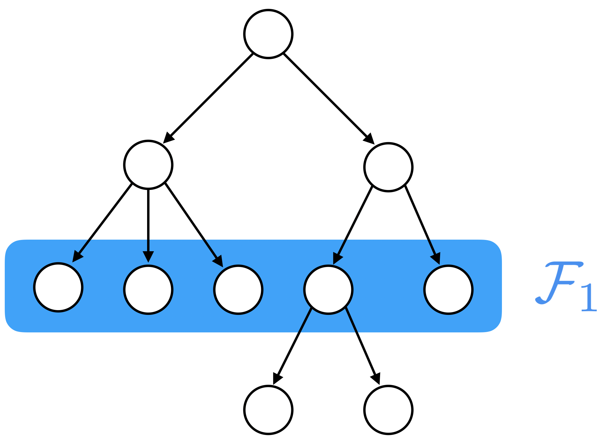
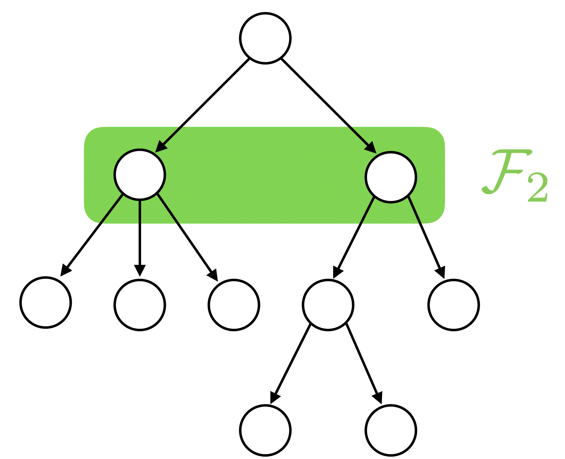
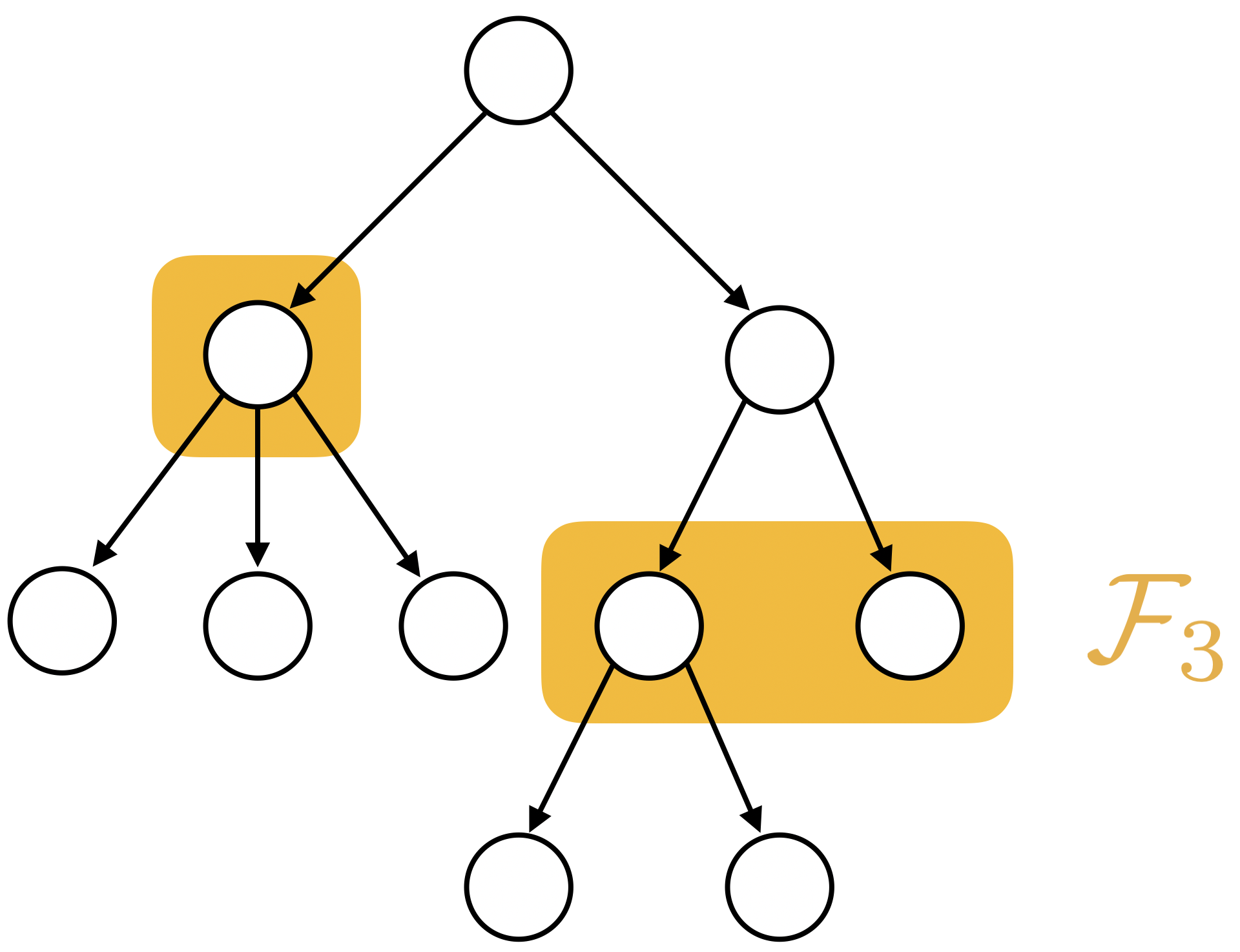
Figure 1: An example of three different frontiers $\mathcal{F}_{1},\mathcal{F}_{2},\mathcal{F}_{3}$ in a single refinement tree.

To lend insight into the structure of frontiers, we provide a characterization of frontiers in terms of incomparable vector spaces. In particular, a frontier $\mathcal{F}$ of a refinement tree $T$ comprises a subset of the vertices $\mathcal{V}$ in which every leaf is descendant from exactly one vertex in $\mathcal{F}$. This can be seen explicitly in fig. 1, which provides examples of frontiers. To show this characterization rigorously, we use the following proposition.

Proposition 3.3 (characterization of frontiers).

Given a $\mathbb{V}$-refinement tree $T\equiv(\mathcal{V},\mathcal{E})$, $\mathcal{F}\subset\mathcal{V}$ is a frontier iff every leaf $\mathbb{L}\in\mathcal{L}$ is descendant from exactly one space $\mathbb{U}\in\mathcal{F}$.

To enable the comparison of two frontiers $\mathcal{F}_{1}$ and $\mathcal{F}_{2}$ such that one can reason about which is ‘finer’, we introduce a natural partial ordering on the set of orthogonal decompositions of $\mathbb{V}$.

Definition 3.6 (partial order $\preceq$).

For two orthogonal decompositions $\mathcal{U}_{1},\mathcal{U}_{2}$ of $\mathbb{V}$, we write $\mathcal{U}_{1}\preceq\mathcal{U}_{2}$ if for every vector space $\mathbb{W}\in\mathcal{U}_{1}$, there is a vector space $\mathbb{U}\in\mathcal{U}_{2}$ such that $\mathbb{W}\subset\mathbb{U}$. If this is the case, we say that $\mathcal{U}_{1}$ is dominated by $\mathcal{U}_{2}$.

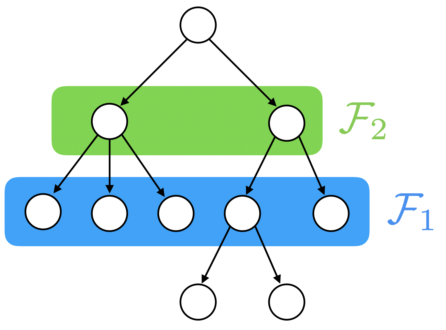
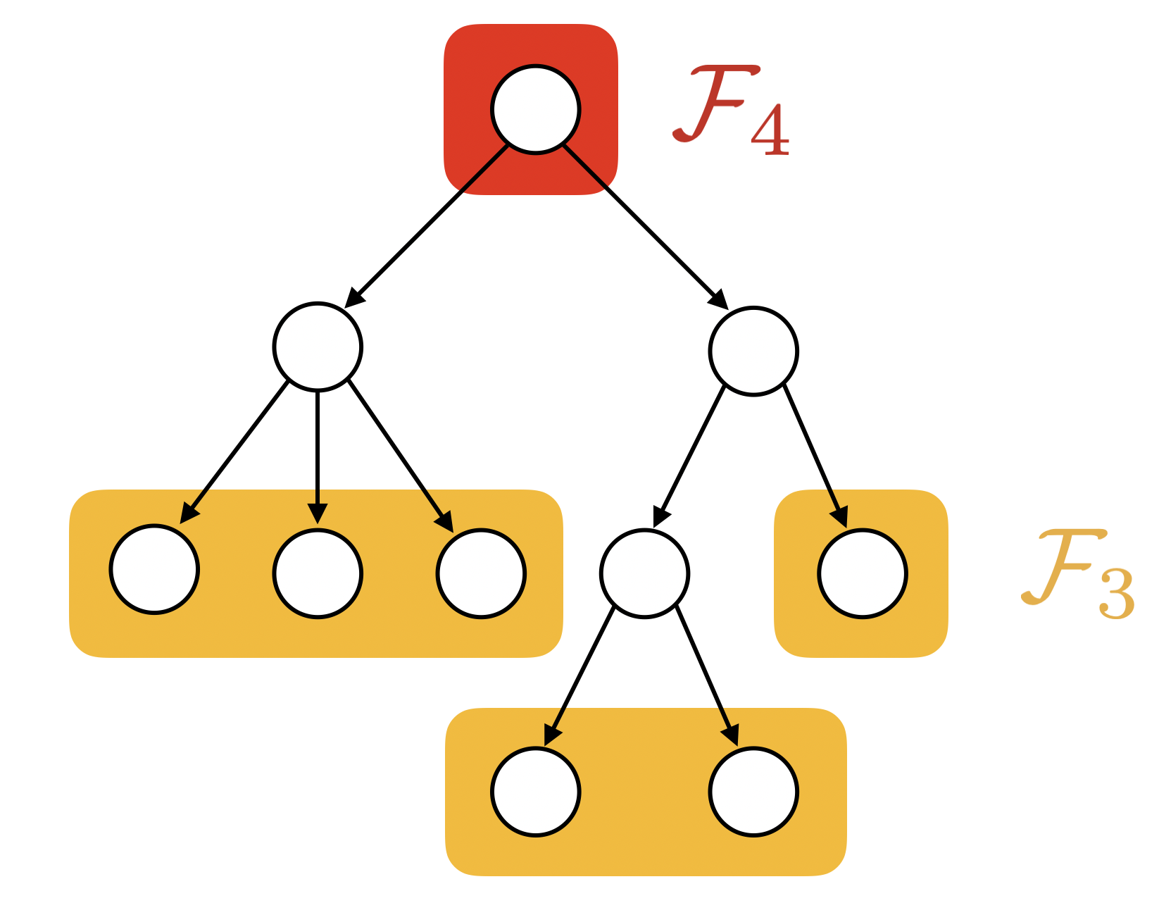
Figure 2: Two examples of the binary relation $\preceq$ of frontiers, as $\mathcal{F}_{1}\preceq\mathcal{F}_{2}$ and $\mathcal{F}_{3}\preceq\mathcal{F}_{4}$. Indeed, all frontiers above are comparable with $\mathcal{F}_{3}\preceq\mathcal{F}_{1}\preceq\mathcal{F}_{2}\preceq\mathcal{F}_{4}$.

This partial ordering extends to frontiers of a refinement tree $T$. Intuitively, $\mathcal{U}_{1}\preceq\mathcal{U}_{2}$ means that $\mathcal{U}_{1}$ is a finer decomposition than $\mathcal{U}_{2}$ and that $\mathcal{U}_{1}$ can be obtained by refining $\mathcal{U}_{2}$. This is borne out by the following proposition.

Proposition 3.4 (ancestor map).

If $\mathcal{U}_{1}$ and $\mathcal{U}_{2}$ are orthogonal decompositions of $\mathbb{V}$ and $\mathcal{U}_{1}\preceq\mathcal{U}_{2}$, then there exists a unique ancestor map $\psi_{\mathcal{U}_{1},\mathcal{U}_{2}}:\mathcal{U}_{1}\longrightarrow\mathcal{U}_{2}$ with the property that $\mathbb{W}\subset\psi_{\mathcal{U}_{1},\mathcal{U}_{2}}(\mathbb{W})$ for $\mathbb{W}\in\mathcal{U}_{1}$. This map also has the property,

$$\mathbb{U}=\sum_{\mathbb{W}\in\psi_{\mathcal{U}_{1},\mathcal{U}_{2}}^{-1}(\mathbb{U})}\mathbb{W},\qquad\forall\mathbb{U}\in\mathcal{U}_{2}\,.$$ (3.22)

We supress the subscripts of the ancestor map when the associated frontiers are obvious from context. Fig. 3 provides a visual example of an ancestor map.

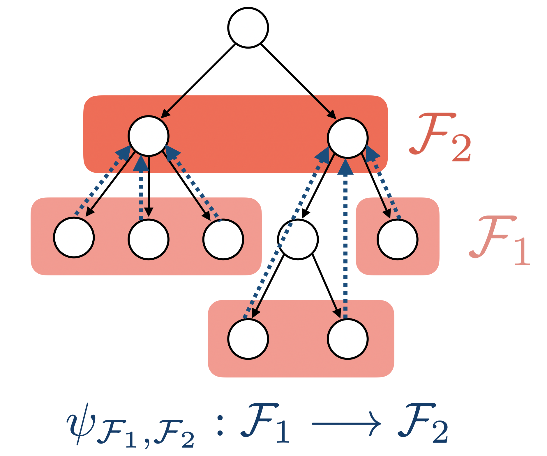
Figure 3: An example of an ancestor map $\psi_{\mathcal{F}_{1},\mathcal{F}_{2}}$ (shown with dotted arrows) where $\mathcal{F}_{1}\preceq\mathcal{F}_{2}$. The ancestor map associates each vertex in $\mathcal{F}_{1}$ with its unique ancestor in $\mathcal{F}_{2}$.

Corollary 3.2.1.

If $\mathcal{U}_{1}\preceq\mathcal{U}_{2}$ are orthogonal decompositions of $\mathbb{V}$ and $\psi_{\mathcal{U}_{1},\mathcal{U}_{2}}$ is the ancestor map between them, then for any vector $\boldsymbol{\phi}\in\mathbb{V}$ and space $\mathbb{U}\in\mathcal{U}_{2}$,

$$P_{\mathbb{U}}(\boldsymbol{\phi})=\sum_{\mathbb{W}\in\psi_{\mathcal{U}_{1},\mathcal{U}_{2}}^{-1}(\mathbb{U})}P_{\mathbb{W}}(\boldsymbol{\phi})\,.$$ (3.23)

Corollary 3.2.2.

If $\mathcal{U}_{1}\preceq\mathcal{U}_{2}$ are orthogonal decompositions of $\mathbb{V}$, then

$$\text{span}(P_{\mathcal{U}_{2}}\left\{\boldsymbol{\phi}\right\})\subset\text{span}(P_{\mathcal{U}_{1}}\left\{\boldsymbol{\phi}\right\})\,.$$ (3.24)

4 Algorithm schema

With mathematical preliminaries now established, we provide an overview of the proposed refinement algorithm. Suppose we are given an initial basis $\mathbf{V}=\mathbf{\Phi}\equiv[\boldsymbol{\phi}_{1}\ \cdots\ \boldsymbol{\phi}_{p_{0}}]\in\mathbb{R}^{n\times p_{0}}_{*}$ as well as an $\mathbb{R}^{n}$-refinement tree $T$. To perform refinement, we maintain a frontier $\mathcal{F}_{i}$ in the tree $T$ for each basis vector $\boldsymbol{\phi}_{i}$, $i=1,\ldots,p_{0}$. Because the basis begins in its initial unrefined state, we initially set all frontiers $\mathcal{F}_{i}$ to the coarsest possible value, namely the root-node state $\mathcal{F}_{i}\leftarrow\{\mathbb{R}^{n}\}$. Now, whenever the ROM solution $\bar{\boldsymbol{x}}+\mathbf{V}\hat{\boldsymbol{x}}^{k}(\boldsymbol{\mu})$ is deemed to be an inaccurate approximation of the FOM solution $\boldsymbol{x}^{k}(\boldsymbol{\mu})$, the algorithm performs basis refinement, which consists of first finding new (finer) frontiers $\mathcal{F}_{i}^{\prime}$, $i=1,\ldots,p_{0}$ satisfying

$$\mathcal{F}_{i}^{\prime}\preceq\mathcal{F}_{i}\,.$$ (4.1)

Next, the algorithm sets $\mathcal{F}_{i}\leftarrow\mathcal{F}_{i}^{\prime}$ and sieves basis vectors $\boldsymbol{\phi}_{i}$ through refined frontier $\mathcal{F}_{i}$ for $i=1,\ldots,p_{0}$ to arrive at a new enriched basis

$$\mathbf{V}=\left[\begin{array}[]{cccc}P_{\mathcal{F}_{1}}\left[\boldsymbol{\phi}_{1}\right]&\ldots&P_{\mathcal{F}_{p_{0}}}\left[\boldsymbol{\phi}_{p_{0}}\right]\end{array}\right]\in\mathbb{R}^{\mathbb{N}(n)\times\bar{\mathcal{F}}}\,,$$ (4.2)

where $\bar{\mathcal{F}}\equiv\bigsqcup_{i}\mathcal{F}_{i}$. If this new enriched basis remains insufficient, we can further refine the frontiers; this can proceed recursively until the desired level of fidelity is achieved. However, we must address three principal problems in developing such an algorithm:

1. Refinement of the frontiers $\mathcal{F}_{i}$ into $\mathcal{F}_{i}^{\prime}$. Ideally, the frontiers $\mathcal{F}_{i}^{\prime}$ would balance the accuracy benefit of increased fidelity with the cost drawback of increased dimensionality. Moreover, the algorithm should determine both (1) the frontiers $\mathcal{F}_{i}$ to refine, and (2) the manner in which they should be refined. For example, in the case of a propagating shock, refinement of the frontiers $\mathcal{F}_{i}$ should be performed in the vicinity of the shock. To address this, we propose an approach that extends the dual-weighted-residual error indicator technique from the original $h$-refinement method [12] to the present framework. These error indicators provide a heuristic guide for assessing which frontiers $\mathcal{F}_{i}$ offer the greatest refinement benefit in terms of minimizing the quantity-of-interest error. Section 5 presents this approach.

2. Construction of the $\mathbb{R}^{n}$-refinement tree $T$. The refinement tree $T$ determines the hierarchical structure of the frontiers $\mathcal{F}_{i}$, and should be designed such that relatively few refinement steps are needed to enable the basis to accurately represent the FOM solution. There are a number of considerations one may want to take into account when constructing this tree. For example, it may be desirable to preserve spatial coherence in the refinement hierarchy of $T$, so that the vector spaces in $\mathcal{V}$ correspond to contiguous regions of the spatial domain; in this case, the refined basis will be sparse, which can improve computational efficiency. Alternatively, it may be desirable to preserve coherence in the frequency domain, or even a combination of the two. In any case, the optimal tree $T$ is clearly highly problem dependent. Nonetheless, we provide a data-driven method for constructing this refinement tree, which is applicable to situations where no such problem-specific information is available besides collected snapshot data. This technique comprises an extension of the recursive $k$-means clustering approach proposed in the original $h$-refinement work [12]. Section 6 presents this approach.

3. Compression of the refined basis $\mathbf{V}$ when necessary. Whenever the basis $\mathbf{V}$ is refined in the above manner, the basis dimension increases. To prevent this dimension from increasing monotonically over time, we require an approach to control the basis dimension. The original $h$-refinement work [12] simply reset the basis $\mathbf{V}$ to the initial basis $\mathbf{\Phi}$ after a prescribed number of time steps. In the present mathematical framework, this corresponds to simply resetting the frontiers $\mathcal{F}_{i}\leftarrow\{\mathbb{R}^{n}\}$ periodically. However, this approach is undesirable for several reasons. First, the fact that the initial basis $\mathbf{\Phi}$ required refinement indicates that it is deficient; resetting the basis simply reintroduces these deficiencies. Second, refining the basis provides valuable information about the particular deficiency of the original basis; resetting the basis effectively discards this important information. To address these drawbacks, we propose to perform an online-efficient POD of solution snapshots computed with the refined ROM (after projecting out solution components in the initial basis $\mathbf{\Phi}$), and subsequently append the resulting POD modes to the original basis $\mathbf{\Phi}$. Naively implemented, this approach incurs an $n$-dependent operation count. However, we have developed an algorithm that employs the structure of the refinement tree $T$ to perform an efficient POD whose operation count depends only on the refined-ROM dimension $p$. Section 7 presents this algorithm.

5 Basis refinement

In this section, we present our approach for refining the frontiers $\mathcal{F}_{i}$, which corresponds to component 1 of the algorithm schema in section 4. This requires additional notation. In particular, we must establish notation for canonical refinements of an arbitrary frontier $\mathcal{F}_{i}$.

5.1 Frontier refinement

First, we define the process of decomposing a vector space $\mathbb{U}$ in a refinement tree $T$.

Definition 5.1 ($T$-refinement).

For a given $\mathbb{V}$-refinement tree $T\equiv(\mathcal{V},\mathcal{E})$, we denote $T$-refinement of a vector space $\mathbb{U}\in\mathcal{V}$ by $R_{T}\left(\mathbb{U}\right)$ and define it as

$$R_{T}\left(\mathbb{U}\right)\equiv\begin{cases}C_{T}(\mathbb{U})&C_{T}(\mathbb{U})\neq\emptyset\\ \{\mathbb{U}\}&\text{otherwise.}\end{cases}$$ (5.1)

Recall that $C_{T}(\mathbb{U})$ denotes the children of $\mathbb{U}$ in tree $T$.

The $T$-refinement of $\mathbb{U}$ corresponds to the decomposition of $\mathbb{U}$ given by the children of $\mathbb{U}$ in the tree $T$, unless $\mathbb{U}$ is a leaf of the tree, in which case the decomposition of $\mathbb{U}$ is given by itself. Now, for any given frontier $\mathcal{F}$ in a $T$-refinement tree, there is a natural notion of the ‘next level’ of refinement. We can simply take the refinement of every subspace in $\mathcal{F}$.

Definition 5.2 (full refinement).

The full refinement $\mathcal{F}^{+}$ of a frontier $\mathcal{F}$ is given by the $T$-refinement of all spaces in $\mathcal{F}$, i.e.,

$$\mathcal{F}^{+}\equiv\bigcup_{\mathbb{U}\in\mathcal{F}}R_{T}\left(\mathbb{U}\right)\,.$$ (5.2)

Figure 4: An example of a full refinement $\mathcal{F}^{+}$ of a frontier $\mathcal{F}$.

Remark 5.1.

Proposition (3.1) implies that $\mathcal{F}^{+}\preceq\mathcal{F}$.

Thus, there is always a simple way to perform refinement of a frontier $\mathcal{F}$: by taking the full refinement $\mathcal{F}^{+}$. However, such a strategy is aggressive; in practice, we aim to consider more tailored refinements of the frontier $\mathcal{F}$. To achieve this, we note that rather than refining every vector space in $\mathcal{F}$, we can refine a subset of these vector spaces. This leads to the definition of a partial refinement of a frontier $\mathcal{F}$.

Definition 5.3 (partial refinement).

The partial refinement of a frontier $\mathcal{F}$ of a $\mathbb{V}$-refinement tree $T$ at vector spaces $\mathbb{U}_{1},\ldots,\mathbb{U}_{m}\in\mathcal{F}$ is given by

$$R_{T}\left(\mathcal{F};\mathbb{U}_{1},\ldots,\mathbb{U}_{m}\right)\equiv\left(\mathcal{F}\setminus\left\{\mathbb{U}_{1},\ldots,\mathbb{U}_{m}\right\}\right)\cup\left(\bigcup_{i=1}^{m}R_{T}\left(\mathbb{U}_{i}\right)\right)\,.$$ (5.3)

In the absence of a refinement tree, the partial refinement of any orthogonal decomposition $\mathcal{U}$ of $\mathbb{V}$ using orthogonal decompositions $\mathcal{U}_{1},\ldots,\mathcal{U}_{m}$ of vector spaces $\mathbb{U}_{1},\ldots,\mathbb{U}_{m}\in\mathcal{U}$ is given by

$$R\left(\mathcal{U};\mathcal{U}_{1},\ldots,\mathcal{U}_{m}\right)\equiv\left(\mathcal{U}\setminus\left\{\mathbb{U}_{1},\ldots,\mathbb{U}_{m}\right\}\right)\cup\left(\bigcup_{i=1}^{m}\mathcal{U}_{i}\right)\,.$$ (5.4)

Remark 5.2.

Note that refinements are always dominated by the original decompositions from which they were refined, i.e.,

$$R_{T}\left(\mathcal{F};\mathbb{U}_{1},\ldots,\mathbb{U}_{m}\right) \preceq\mathcal{F}\,,$$ (5.5)

$$R\left(\mathcal{U};\mathcal{U}_{1},\ldots\mathcal{U}_{m}\right) \preceq\mathcal{U}\,.$$ (5.6)

Remark 5.3.

The partial refinement $R_{T}\left(\mathcal{F};\mathbb{U}_{1},\ldots,\mathbb{U}_{m}\right)$ of a frontier $\mathcal{F}$ at vector spaces $\mathbb{U}_{1},\ldots,\mathbb{U}_{m}\in\mathcal{F}$ is also a frontier. Moreover, if $\mathcal{F}_{1},\ldots,\mathcal{F}_{m}$ are frontiers of the subtrees of $T$ rooted at $\mathbb{U}_{1},\ldots,\mathbb{U}_{m}\in\mathcal{F}$, respectively, then the partial refinement $R\left(\mathcal{F};\mathcal{F}_{1},\ldots,\mathcal{F}_{m}\right)$ is also a frontier.

5.2 Dual-weighted-residual error indicators

The workhorse of the refinement portion of our algorithm is the goal-oriented dual-weighted-residual error-indicator approach from the original $h$-refinement method [12]. This approach ascribes an error indicator to every element of a frontier $\mathcal{F}$, thereby enabling the method to refine only the elements of the frontier $\mathcal{F}$ associated with the largest approximated errors.

We begin by assuming the context of section 4, i.e., we are given an initial basis $\mathbf{V}=\mathbf{\Phi}\equiv[\boldsymbol{\phi}_{1}\ \cdots\ \boldsymbol{\phi}_{p_{0}}]\in\mathbb{R}^{n\times p_{0}}_{*}$ and an $\mathbb{R}^{n}$-refinement tree $T$. The current ‘coarse’ basis is given by the sieve of the basis vectors $\boldsymbol{\phi}_{1},\ldots,\boldsymbol{\phi}_{p_{0}}$ through frontiers $\mathcal{F}_{1},\ldots,\mathcal{F}_{p_{0}}$, i.e.,

$$\mathbf{V}^{H}=\left[\begin{array}[]{ccc}P_{\mathcal{F}_{1}}\left[\boldsymbol{\phi}_{1}\right]&\cdots&P_{\mathcal{F}_{p_{0}}}\left[\boldsymbol{\phi}_{p_{0}}\right]\end{array}\right]\in\mathbb{R}^{\mathbb{N}(n)\times\bar{\mathcal{F}}^{H}}\,,$$ (5.7)

where $\bar{\mathcal{F}}^{H}\equiv\bigsqcup_{i}\mathcal{F}_{i}$. If the coarse basis $\mathbf{V}^{H}$ is deficient, we would like enrich the basis $\mathbf{V}^{H}$ by refining the frontiers $\mathcal{F}_{1},\ldots,\mathcal{F}_{p_{0}}$. A naive way to perform this refinement would be simply to apply full refinement to each frontier $\mathcal{F}_{1},\ldots,\mathcal{F}_{p_{0}}$, i.e.,

$$\mathbf{V}^{h}\equiv\left[\begin{array}[]{ccc}P_{\mathcal{F}_{1}^{+}}\left[\boldsymbol{\phi}_{1}\right]&\cdots&P_{\mathcal{F}_{p_{0}}^{+}}\left[\boldsymbol{\phi}_{p_{0}}\right]\end{array}\right]\in\mathbb{R}^{\mathbb{N}(n)\times\bar{\mathcal{F}}^{h}}\,,$$ (5.8)

where $\bar{\mathcal{F}}^{h}\equiv\bigsqcup_{i}\mathcal{F}_{i}^{+}$ and $\mathbf{V}^{h}$ denotes the full refinement of the previous basis $\mathbf{V}^{H}$. This aggressive approach is tantamount to performing uniform refinement. Instead, we aim to devise an adaptive approach that performs refinement only on basis vectors contributing most to the quantity-of-interest error.

For each frontier $\mathcal{F}_{i}$ in Eq. (5.7) and its full refinement $\mathcal{F}_{i}^{+}$, there exists an ancestor map

$$\psi_{i}\equiv\psi_{i,\mathcal{F}_{i}^{+},\mathcal{F}_{i}}:\mathcal{F}_{i}^{+}\longrightarrow\mathcal{F}_{i}\,.$$ (5.9)

These ancestor maps together induce a global ancestor map from $\bar{\mathcal{F}}^{h}\equiv\bigsqcup_{i}\mathcal{F}_{i}^{+}$ to $\bar{\mathcal{F}}^{H}\equiv\bigsqcup_{i}\mathcal{F}_{i}$, i.e.,

$$\psi\equiv\psi_{\bar{\mathcal{F}}^{h},\bar{\mathcal{F}}^{H}}:\bar{\mathcal{F}}^{h}\longrightarrow\bar{\mathcal{F}}^{H}$$ (5.10)

such that $\left.\psi\right|_{\mathcal{F}_{i}^{+}}=\psi_{i}$. The indicator matrix $\mathbf{I}^{h}_{H}\in\mathbb{R}^{\bar{\mathcal{F}}^{h}\times\bar{\mathcal{F}}^{H}}$ for this global ancestor map has entries

$$\left(\mathbf{I}^{h}_{H}\right)_{\mathbb{W},\mathbb{U}}\equiv\begin{cases}1&\psi(\mathbb{W})=\mathbb{U}\\ 0&\text{otherwise.}\end{cases}$$ (5.11)

In analogue to the prolongation operator from $h$-refinement for finite elements, we refer to the matrix $\mathbf{I}^{h}_{H}$ as the prolongation operator from the coarse basis $\mathbf{V}^{H}$ to the fine basis $\mathbf{V}^{h}$. Indeed, corollary (3.2.1) implies

$$\mathbf{V}^{H}=\mathbf{V}^{h}\mathbf{I}^{h}_{H}\,.$$ (5.12)

The prolongation operator relates coordinate representations in the coarse basis $\mathbf{V}^{H}$ to coordinate representations in the fine basis $\mathbf{V}^{h}$. Indeed, if we have a coordinate representation $\hat{\boldsymbol{x}}^{H}$ of data $\mathbf{V}^{H}\hat{\boldsymbol{x}}^{H}$ in the coarse basis $\mathbf{V}^{H}$, then

$$\mathbf{V}^{H}\hat{\boldsymbol{x}}^{H}=(\mathbf{V}^{h}\mathbf{I}^{h}_{H})\hat{\boldsymbol{x}}^{H}=\mathbf{V}^{h}(\mathbf{I}^{h}_{H}\hat{\boldsymbol{x}}^{H})\,.$$ (5.13)

Hence, $\mathbf{I}^{h}_{H}\hat{\boldsymbol{x}}^{H}$ provides the coordinate representation of this data in the fine basis $\mathbf{V}^{h}$.

Now, consider the context of refinement. Suppose we have computed a (coarse) ROM solution $\mathbf{V}^{H}\hat{\boldsymbol{x}}^{H}$ satisfying

$$\left(\mathbf{V}^{H}\right)^{T}\boldsymbol{r}\left(\mathbf{V}^{H}\hat{\boldsymbol{x}}^{H}\right)={\mathbf{0}}\,.$$ (5.14)

If we perform uniform refinement of all frontiers and solve the ROM corresponding to the resulting fine basis $\mathbf{V}^{h}$, we obtain a higher fidelity ROM solution $\mathbf{V}^{h}\hat{\boldsymbol{x}}^{h}$ satisfying

$$\left(\mathbf{V}^{h}\right)^{T}\boldsymbol{r}\left(\mathbf{V}^{h}\hat{\boldsymbol{x}}^{h}\right)={\mathbf{0}}\,.$$ (5.15)

However, we would like to avoid computations that scale with the dimension of the fully refined basis.

To achieve this—yet still glean information about the unknown refined solution $\mathbf{V}^{h}\hat{\boldsymbol{x}}^{h}$—we apply dual-weighted-residual error estimation. We begin by assuming the residual $\boldsymbol{r}$ is twice continuously differentiable and approximate it using a first-order Taylor-series expansion about the known coarse solution $\mathbf{V}^{H}\hat{\boldsymbol{x}}^{H}$, i.e.,

$$\boldsymbol{r}\left(\mathbf{V}^{h}\hat{\boldsymbol{x}}^{h}\right)=\boldsymbol{r}(\mathbf{V}^{H}\hat{\boldsymbol{x}}^{H})+\frac{\partial\boldsymbol{r}}{\partial\boldsymbol{x}}\left(\mathbf{V}^{H}\hat{\boldsymbol{x}}^{H}\right)\mathbf{V}^{h}\left(\hat{\boldsymbol{x}}^{h}-\mathbf{I}^{h}_{H}\hat{\boldsymbol{x}}^{H}\right)+O(\|\hat{\boldsymbol{x}}^{h}-\mathbf{I}^{h}_{H}\hat{\boldsymbol{x}}^{H}\|^{2})\,,$$ (5.16)

where we have used Eq. (5.12) to relate the coarse and refined bases. Left multiplying the above by $\mathbf{V}^{h}$ and using Eq. (5.15) yields

$${\mathbf{0}}=(\mathbf{V}^{h})^{T}\boldsymbol{r}\left(\mathbf{V}^{h}\hat{\boldsymbol{x}}^{h}\right)=(\mathbf{V}^{h})^{T}\boldsymbol{r}(\mathbf{V}^{H}\hat{\boldsymbol{x}}^{H})+(\mathbf{V}^{h})^{T}\frac{\partial\boldsymbol{r}}{\partial\boldsymbol{x}}\left(\mathbf{V}^{H}\hat{\boldsymbol{x}}^{H}\right)\mathbf{V}^{h}\left(\hat{\boldsymbol{x}}^{h}-\mathbf{I}^{h}_{H}\hat{\boldsymbol{x}}^{H}\right)+O(\|\hat{\boldsymbol{x}}^{h}-\mathbf{I}^{h}_{H}\hat{\boldsymbol{x}}^{H}\|^{2})\,.$$ (5.17)

Solving for the error $\hat{\boldsymbol{x}}^{h}-\mathbf{I}^{h}_{H}\hat{\boldsymbol{x}}^{H}$ gives the Newton approximation

$$\left(\hat{\boldsymbol{x}}^{h}-\mathbf{I}^{h}_{H}\hat{\boldsymbol{x}}^{H}\right)=-\left[(\mathbf{V}^{h})^{T}\frac{\partial\boldsymbol{r}}{\partial\boldsymbol{x}}\left(\mathbf{V}^{H}\hat{\boldsymbol{x}}^{H}\right)\mathbf{V}^{h}\right]^{-1}\left(\mathbf{V}^{h}\right)^{T}\boldsymbol{r}(\mathbf{V}^{H}\hat{\boldsymbol{x}}^{H})+O(\|\hat{\boldsymbol{x}}^{h}-\mathbf{I}^{h}_{H}\hat{\boldsymbol{x}}^{H}\|^{2})\,.$$ (5.18)

Unfortunately, computing this Newton approximation requires a $\bar{\mathcal{F}}^{h}\times\bar{\mathcal{F}}^{h}$ linear-system solve; this is precisely what we aim to avoid. Thus, we instead consider the dual. As above, we assume the quantity-of-interest functional $g$ (see Eq. (2.2)) is twice continuously differentiable and perform a Taylor expansion about the coarse solution $\hat{\boldsymbol{x}}^{H}$, i.e.,

$$g(\mathbf{V}^{h}\hat{\boldsymbol{x}}^{h})=g(\mathbf{V}^{H}\hat{\boldsymbol{x}}^{H})+\frac{\partial g}{\partial\boldsymbol{x}}\left(\mathbf{V}^{H}\hat{\boldsymbol{x}}^{H}\right)\mathbf{V}^{h}\left(\hat{\boldsymbol{x}}^{h}-\mathbf{I}^{h}_{H}\hat{\boldsymbol{x}}^{H}\right)+O(\|\hat{\boldsymbol{x}}^{h}-\mathbf{I}^{h}_{H}\hat{\boldsymbol{x}}^{H}\|^{2})\,.$$ (5.19)

Substituting Eq. (5.18) into Eq. (5.19) yields

$$g(\mathbf{V}^{h}\hat{\boldsymbol{x}}^{h})-g(\mathbf{V}^{H}\hat{\boldsymbol{x}}^{H})=-\left(\hat{\mathbf{y}}^{h}\right)^{T}(\mathbf{V}^{h})^{T}\boldsymbol{r}(\mathbf{V}^{H}\hat{\boldsymbol{x}}^{H})+O(\|\hat{\boldsymbol{x}}^{h}-\mathbf{I}^{h}_{H}\hat{\boldsymbol{x}}^{H}\|^{2})\,,$$ (5.20)

where $\hat{\mathbf{y}}^{h}\in\mathbb{R}^{\bar{\mathcal{F}}^{h}}$ is the fine adjoint satisfying

$$\left[(\mathbf{V}^{h})^{T}\frac{\partial\boldsymbol{r}}{\partial\boldsymbol{x}}(\mathbf{V}^{H}\hat{\boldsymbol{x}}^{H})^{T}\mathbf{V}^{h}\right]^{T}\hat{\mathbf{y}}^{h}=(\mathbf{V}^{h})^{T}\frac{\partial g}{\partial\boldsymbol{x}}\left(\mathbf{V}^{H}\hat{\boldsymbol{x}}^{H}\right)^{T}\,.$$ (5.21)

It may not seem that we have made any progress, as computing the adjoint $\hat{\mathbf{y}}^{h}$ in satisfying (5.21) still requires a $\bar{\mathcal{F}}^{h}\times\bar{\mathcal{F}}^{h}$ linear-system solve. However, the advantage of adopting this viewpoint is that there is a natural way to approximate the adjoint $\hat{\mathbf{y}}^{h}$ in an efficient manner, namely as the prolongation of the coarse adjoint $\hat{\mathbf{y}}^{H}\in\mathbb{R}^{\bar{\mathcal{F}}^{H}}$, i.e.,

$$\hat{\mathbf{y}}^{h}_{H}\equiv\mathbf{I}^{h}_{H}\hat{\mathbf{y}}^{H}\,.$$ (5.22)

where the coarse adjoint $\hat{\mathbf{y}}^{H}$ satisfies

$$\left[(\mathbf{V}^{H})^{T}\frac{\partial\boldsymbol{r}}{\partial\boldsymbol{x}}(\mathbf{V}^{H}\hat{\boldsymbol{x}}^{H})^{T}\mathbf{V}^{H}\right]^{T}\hat{\mathbf{y}}^{H}=(\mathbf{V}^{H})^{T}\frac{\partial g}{\partial\boldsymbol{x}}\left(\mathbf{V}^{H}\hat{\boldsymbol{x}}^{H}\right)^{T}\,.$$ (5.23)

Critically, computing the coarse adjoint $\hat{\mathbf{y}}^{H}$ requires only a $\bar{\mathcal{F}}^{H}\times\bar{\mathcal{F}}^{H}$ linear-system solve. Replacing the fine adjoint $\hat{\mathbf{y}}^{h}$ with its approximation $\hat{\mathbf{y}}^{h}_{H}$ in Eq. (5.20) yields

$$g\left(\mathbf{V}^{h}\hat{\boldsymbol{x}}^{h}\right)-g\left(\mathbf{V}^{H}\hat{\boldsymbol{x}}^{H}\right)\approx-\left(\hat{\mathbf{y}}^{h}_{H}\right)^{T}(\mathbf{V}^{h})^{T}\boldsymbol{r}\left(\mathbf{V}^{H}\hat{\boldsymbol{x}}^{H}\right)\,.$$ (5.24)

Finally, we can bound the right hand side of Eq. (5.24) by

$$\left|\left(\hat{\mathbf{y}}^{h}_{H}\right)^{T}(\mathbf{V}^{h})^{T}\boldsymbol{r}\left(\mathbf{V}^{H}\hat{\boldsymbol{x}}^{H}\right)\right|\leq\sum_{\mathbb{W}\in\bar{\mathcal{F}}^{h}}\boldsymbol{\delta}^{h}_{\mathbb{W}}\,.$$ (5.25)

Here, the error indicators $\boldsymbol{\delta}^{h}_{\mathbb{W}}\in\mathbb{R}_{\geq 0}$ for $\mathbb{W}\in\bar{\mathcal{F}}^{h}$ are the absolute values of the summands in the inner product $\left(\hat{\mathbf{y}}^{h}_{H}\right)^{T}\left[(\mathbf{V}^{h})^{T}\boldsymbol{r}\left(\mathbf{V}^{H}\hat{\boldsymbol{x}}^{H}\right)\right]$, i.e.,

$$\boldsymbol{\delta}^{h}_{\mathbb{W}}\equiv\left|\left[\hat{\mathbf{y}}^{h}_{H}\right]_{\mathbb{W}}\left(\boldsymbol{v}_{\mathbb{W}}^{h}\right)^{T}\boldsymbol{r}\left(\mathbf{V}^{H}\hat{\boldsymbol{x}}^{H}\right)\right|\,,$$ (5.26)

where $\boldsymbol{v}_{\mathbb{W}}^{h}$ denotes the $\mathbb{W}$-column of $\mathbf{V}^{h}$. These error indicators ascribe an approximate error heuristic to every element in the full refinement $\bar{\mathcal{F}}^{h}$. Moreover, these error indicators can be pulled back to the global coarse frontier $\bar{\mathcal{F}}^{H}$ via the global ancestor map $\psi$, i.e.,

$$\boldsymbol{\delta}^{H}_{\mathbb{U}}\equiv\sum_{\mathbb{W}\in\psi^{-1}(\mathbb{U})}\boldsymbol{\delta}^{h}_{\mathbb{W}},\qquad\mathbb{U}\in\bar{\mathcal{F}}^{H}\,.$$ (5.27)

That is, the error indicator for $\mathbb{U}\in\bar{\mathcal{F}}^{H}$ comprises the sum of error indicators of its children. In matrix form, this corresponds to

$$\boldsymbol{\delta}^{H}=\boldsymbol{\delta}^{h}\mathbf{I}^{h}_{H}\,.$$ (5.28)

The key to our refinement algorithm is to refine only the spaces $\mathbb{U}\in\bar{\mathcal{F}}^{H}$ for which the corresponding error indicator $\boldsymbol{\delta}^{H}_{\mathbb{U}}$ is large. In our implementation, we refine those spaces $\mathbb{U}\in\bar{\mathcal{F}}^{H}$ such that the corresponding error indicator is greater than the average of all error indicators. Algorithm 1 provides the full procedure for computing these error indicators.

Algorithm 1 Computation of Error Indicators

Input: The current coarse basis $\mathbf{V}^{H}$, the current frontiers $\mathcal{F}_{1},\ldots,\mathcal{F}_{p_{0}}$
      Output: The fine error indicators $\boldsymbol{\delta}^{h}$.

1:procedure ComputeErrorIndicators($\mathbf{V}^{H}$, $\mathcal{F}_{1},\ldots,\mathcal{F}_{p_{0}}$)

2:     $\bar{\mathcal{F}}^{H}\leftarrow\bigsqcup_{i}\mathcal{F}_{i}$

3:     $\bar{\mathcal{F}}^{h}\leftarrow\bigsqcup_{i}\mathcal{F}^{+}_{i}$

4:     $\mathbf{I}^{h}_{H}\leftarrow\textsc{ComputeProlongationOperator}\left(\bar{\mathcal{F}}^{H},\bar{\mathcal{F}}^{h}\right)$ $\triangleright$ Compute prolongation operator using Eq. (5.11)

5:      $\hat{\mathbf{y}}^{H}\leftarrow\left[(\mathbf{V}^{H})^{T}\frac{\partial\boldsymbol{r}}{\partial\boldsymbol{x}}(\mathbf{V}^{H}\hat{\boldsymbol{x}}^{H})^{T}\mathbf{V}^{H}\right]^{-T}\left[(\mathbf{V}^{H})^{T}\frac{\partial g}{\partial\boldsymbol{x}}\left(\mathbf{V}^{H}\hat{\boldsymbol{x}}^{H}\right)^{T}\right]$ $\triangleright$ Compute the coarse adjoint using Eq. (5.23)

6:     $\hat{\mathbf{y}}^{h}_{H}\leftarrow\mathbf{I}^{h}_{H}\hat{\mathbf{y}}^{H}$ $\triangleright$ Prolongate coarse adjoint to fine coordinate space.

7:     $\boldsymbol{\delta}^{h}\leftarrow\boldsymbol{0}\in\mathbb{R}^{\bar{\mathcal{F}}^{h}}$

8:     for $\mathbb{W}\in\bar{\mathcal{F}}^{h}\setminus\mathcal{L}$ do

9:         $\boldsymbol{\delta}^{h}_{\mathbb{W}}\leftarrow\left|\left[\hat{\mathbf{y}}^{h}_{H}\right]_{\mathbb{W}}\left(\boldsymbol{v}_{\mathbb{W}}^{h}\right)^{T}\boldsymbol{r}\left(\mathbf{V}^{H}\hat{\boldsymbol{x}}^{H}\right)\right|$$\triangleright$ Compute the error indicators using Eq. (5.26)

10:     end for

11:     return $\boldsymbol{\delta}^{h}$

12:end procedure

5.3 Refinement algorithm

With the preliminaries of frontier refinement and dual-weighted-residual error indicators now established, we return to the objective of this work: adaptive basis refinement.

Algorithms 2 and 3 report the proposed refinement algorithm, which takes the following approach: at a given time instance, the method first solves the ROM equations to within a prescribed tolerance $\varepsilon_{ROM}$. Next, an error indicator is applied to the ROM solution to assess its accuracy; here, we take the error indicator to be the norm of the FOM residual evaluated at the ROM solution. If this error indicator is larger than a prescribed tolerance $\varepsilon$, then the algorithm performs basis refinement. This is repeated until either the ROM solution satisfies the error-indicator tolerance, or the ROM has converged to the FOM.

Algorithm 2 Computation of Refined Frontiers

Input: The $\mathbb{R}^{n}$-refinement tree $T$, the fine error indicators $\boldsymbol{\delta}^{h}$, the current frontiers $\mathcal{F}_{1},\ldots,\mathcal{F}_{p_{0}}$.
      Output: A new set of frontiers $\mathcal{F}_{1}^{\prime},\ldots,\mathcal{F}_{p_{0}}^{\prime}$ refined according to the input error indicators.

1:procedure RefineFrontiers($T,\boldsymbol{\delta}^{h},\mathcal{F}_{1},\ldots,\mathcal{F}_{p_{0}}$)

2:     $\bar{\mathcal{F}}^{H}\leftarrow\bigsqcup_{i}\mathcal{F}_{i}$

3:     $\bar{\mathcal{F}}^{h}\leftarrow\bigsqcup_{i}\mathcal{F}^{+}_{i}$

4:     $\psi\leftarrow\textsc{GetGlobalAncestorMap}\left(\bar{\mathcal{F}}^{h},\bar{\mathcal{F}}^{H}\right)$ $\triangleright$ Compute the map in Eq. (5.10) sending every space to its ancestor.

5:     $\mathbf{I}^{h}_{H}\leftarrow\textsc{ComputeProlongationOperator}\left(\bar{\mathcal{F}}^{H},\bar{\mathcal{F}}^{h}\right)$ $\triangleright$ Compute prolongation operator using Eq. (5.11).

6:     $\boldsymbol{\delta}^{H}=\boldsymbol{\delta}^{h}\mathbf{I}^{h}_{H}$ $\triangleright$ Compute coarse error indicators using Eq. (5.28).

7:     $\eta\leftarrow\frac{1}{|\bar{\mathcal{F}}^{H}|}\sum_{\mathbb{U}\in\bar{\mathcal{F}}^{H}}\boldsymbol{\delta}^{H}_{\mathbb{U}}$ $\triangleright$ Compute the average of the coarse error indicators.

8:     $S\leftarrow\{\mathbb{U}\in\bar{\mathcal{F}}^{H}\mid\boldsymbol{\delta}^{H}_{\mathbb{U}}\geq\eta\}$ $\triangleright$ Select the spaces in $\bar{\mathcal{F}}^{H}$ whose coarse error indicator is greater than average.

9:     for $i\in\mathbb{N}(p_{0})$ do $\triangleright$ For each frontier $\mathcal{F}_{i}$

10:         $S_{i}\leftarrow\mathcal{F}_{i}\cap S$ $\triangleright$ Extract the elements of $S$ that came from $\mathcal{F}_{i}$.

11:         $\mathcal{F}_{i}^{\prime}\leftarrow R_{T}\left(\mathcal{F};S_{i}\right)$ $\triangleright$ Refine the frontier $\mathcal{F}_{i}$ at these spaces.

12:     end for

13:     return $(\mathcal{F}_{1}^{\prime},\ldots,\mathcal{F}_{p_{0}}^{\prime})$ $\triangleright$ Return the refined frontiers.

14:end procedure

Algorithm 3 Refinement Algorithm

Input: $\mathbb{R}^{n}$-refinement tree $T$, initial basis $\mathbf{\Phi}$, current frontiers $\mathcal{F}_{1},\ldots,\mathcal{F}_{p_{0}}$, reference solution $\bar{\boldsymbol{x}}$, residual function $\boldsymbol{r}$, ROM-residual tolerance $\varepsilon_{ROM}$, and FOM-residual tolerance $\varepsilon$.
      Output: A new set of frontiers $\mathcal{F}_{1}^{\prime},\ldots,\mathcal{F}_{p_{0}}^{\prime}$ refined according to the input error indicators.

1:procedure SolveModel($T,\mathbf{\Phi},\mathcal{F}_{1},\ldots,\mathcal{F}_{p_{0}},\bar{\boldsymbol{x}},\varepsilon_{ROM},\varepsilon$)

2:     while True do $\triangleright$ Refine the basis until the specified full-order tolerance is met.

3:          $\mathbf{V}^{H}\leftarrow\left[\begin{array}[]{ccc}P_{\mathcal{F}_{1}}\left[\boldsymbol{\phi}_{1}\right]&\cdots&P_{\mathcal{F}_{p_{0}}}\left[\boldsymbol{\phi}_{p_{0}}\right]\end{array}\right]$ $\triangleright$ Retrieve the current coarse model basis.

4:         $\hat{\boldsymbol{x}}\leftarrow\textsc{SolveROM}(\boldsymbol{r},\mathbf{V}^{H},\bar{\boldsymbol{x}},\varepsilon_{ROM})$ $\triangleright$ Solve the system $(\mathbf{V}^{H})^{T}\boldsymbol{r}\left(\bar{\boldsymbol{x}}+\mathbf{V}^{H}\hat{\boldsymbol{x}}\right)=0$ from Eq. (2.5).

5:         $\boldsymbol{x}\leftarrow\mathbf{V}^{H}\hat{\boldsymbol{x}}$ $\triangleright$ Lift the result to the full-order model.

6:         if $\|\boldsymbol{r}(\boldsymbol{x})\|_{2}<\varepsilon$ then $\triangleright$ Check if the full-order residual is within the specified tolerance.

7:              break $\triangleright$ If the specified tolerance is satisfied, stop refinement.

8:         end if

9:          $\boldsymbol{\delta}^{h}\leftarrow\textsc{ComputeErrorIndicators}(\mathbf{V}^{H},\mathcal{F}_{1},\ldots,\mathcal{F}_{p_{0}})$ $\triangleright$ Compute the error indicators in Eq. (5.26).

10:          $(\mathcal{F}_{1},\ldots,\mathcal{F}_{p_{0}})\leftarrow\textsc{RefineFrontiers}(T,\boldsymbol{\delta}^{h},\mathcal{F}_{1},\ldots,\mathcal{F}_{p_{0}})$ $\triangleright$ Use error indicators to selectively refine frontiers.

11:     end while

12:     return $(\mathcal{F}_{1},\ldots,\mathcal{F}_{p_{0}},\hat{\boldsymbol{x}})$.

13:end procedure

5.4 Resolving ill-conditioning and ensuring linear independence

To complete the presentation of the refinement algorithm, we must address two outstanding problems:

1. The refinement algorithm does not formally ensure that the matrix $\mathbf{V}$ is indeed a basis, i.e., that $\mathbf{V}$ has full column rank and thus belongs to the non-compact Stiefel manifold.

2. The refinement algorithm does not ensure the matrix $\mathbf{V}$ is well conditioned, even if it has full column rank. This occurs because every vector-space sieve reduces the $\ell^{2}$-norm of some columns of $\mathbf{V}$, as

   $$\|\boldsymbol{\phi}\|_{2}^{2}=\sum_{\boldsymbol{\phi}_{i}\in P_{\mathcal{U}}\left\{\boldsymbol{\phi}\right\}}\|\boldsymbol{\phi}_{i}\|_{2}^{2}\,.$$ (5.29)

   Therefore, recursive unbalanced basis refinement will cause the $\ell^{2}$-norms of some columns of $\mathbf{V}$ to shrink, which could lead to poor conditioning.

To counteract the first issue, we follow the approach of the original ROM $h$-refinement method [12] and deactivate redundant vectors of $\mathbf{V}\equiv[\boldsymbol{v}_{1}\ \cdots\ \boldsymbol{v}_{p}]$ by using a column-pivoted QR factorization. We address the second issue by scaling the remaining basis vectors to ensure the basis is well-conditioned. This amounts to computing a diagonal scaling matrix $\mathbf{\Sigma}_{*}\in\mathbb{R}^{p_{*}\times p_{*}}$ and a selection matrix $\mathbf{P}\in\{0,1\}^{p\times p_{*}}$, and defining

$$\mathbf{V}_{*}\equiv\mathbf{V}\mathbf{P}\mathbf{\Sigma}_{*}$$ (5.30)

such the basis $\mathbf{V}_{*}\in\mathbb{R}^{n\times p_{*}}_{*}$ contains a subset of the (scaled) columns of $\mathbf{V}$. To compute $\mathbf{P}$ and $\mathbf{\Sigma}_{*}$, we first define a general diagonal rescaling matrix $\mathbf{\Sigma}\in\mathbb{R}^{p\times p}$ with diagonal entries $\mathbf{\Sigma}_{ii}\equiv{1}/{\|\boldsymbol{v}_{i}\|_{2}}$. This addresses the second issue above. However, to address the first issue, we must cull the redundant columns of $\mathbf{V}\mathbf{\Sigma}$ to ensure linear independence to within some tolerance. We accomplish this via a column-pivoted QR decomposition

$$\mathbf{Q}\mathbf{R}\mathbf{\Pi}=\mathbf{V}\mathbf{\Sigma}\,.$$ (5.31)

Denoting by $\epsilon_{\text{QR}}$ the desired tolerance for linear independence, we select the columns of $\mathbf{V}$ whose diagonal $\mathbf{R}$-factors are greater than $\epsilon_{\text{QR}}$; we denote the associated cutoff by $s\vcentcolon=\min_{i}\{\mathbf{R}_{ii}<\epsilon_{\text{QR}}\}$. The selection operator $\mathbf{P}$ then corresponds to the first $s$ columns of the pivoting matrix, i.e.,

$$\mathbf{P}\equiv\mathbf{\Pi}_{:,\mathbb{N}(s)}\,.$$ (5.32)

Likewise, to preserve the rescaling factors for the preserved columns, we set

$$\mathbf{\Sigma}_{*}=\mathbf{P}^{T}\mathbf{\Sigma}\mathbf{P}\,.$$ (5.33)

These choices for $\mathbf{P}$ and $\mathbf{\Sigma}_{*}$ yield a basis $\mathbf{V}_{*}$ defined by Eq. (5.30) that is both linearly independent and well conditioned according to the threshold $\epsilon_{\text{QR}}$.

In the context of algorithm 3, we perform this excision procedure after performing frontier refinement. We then mark the frontier nodes corresponding to the excised columns of $\mathbf{V}$ as inactive, after which point the excised basis vectors are effectively ignored and can no longer be refined. These modifications can be incorporated in the refinement algorithm 3 with only minimal changes.

5.5 Proof of monotone convergence

To conclude this section, we demonstrate that the proposed basis-refinement algorithm ensures the ROM converges to the FOM, and that the refined bases produce a monotone sequence of embedded subspaces.

Theorem 5.4 (Convergence to the full-order model).

If for every leaf $\mathbb{L}\in\mathcal{L}$ of the refinement tree $T$, there exists an initial ROM basis vector $\boldsymbol{\phi}_{i(\mathbb{L})}$ such that $P_{\mathbb{L}}(\boldsymbol{\phi}_{i(\mathbb{L})})\neq 0$, then one of the following must occur:

1. The refinement algorithm computes a solution satisfying the FOM equations to within tolerance $\varepsilon$.

2. The range of the refined basis converges to $\mathbb{R}^{n}$.

Proof.

Consider the event where $\mathcal{F}_{i}=\mathcal{L}$, $i=1,\ldots,p_{0}$. In this event, for each $\mathbb{L}\in\mathcal{L}$, the projected vector $P_{\mathbb{L}}(\boldsymbol{\phi}_{i(\mathbb{L})})\in\mathbb{L}$ is nonzero by assumption, and $\mathbb{L}$ has dimension $1$, so $P_{\mathbb{L}}(\boldsymbol{\phi}_{i(\mathbb{L})})$ spans $\mathbb{L}$ and

$$\mathbb{L}\subset\text{span}(P_{\mathbb{L}}(\boldsymbol{\phi}_{i(\mathbb{L})}))\subset\text{span}\left(P_{\mathcal{F}_{i(\mathbb{L})}}\left\{\boldsymbol{\phi}_{i(\mathbb{L})}\right\}\right)\subset\text{span}\left(\bigcup_{i=1}^{p_{0}}P_{\mathcal{F}_{i}}\left\{\boldsymbol{\phi}_{i}\right\}\right)=\text{range}(\mathbf{V})\,.$$ (5.34)

Summing over $\mathbb{L}\in\mathcal{L}$ then gives us

$$\mathbb{R}^{n}=\sum_{\mathbb{L}\in\mathcal{L}}\mathbb{L}\subset\text{range}(\mathbf{V})\,.$$ (5.35)

Thus, if the event $\mathcal{F}_{i}=\mathcal{L}$, $i=1,\ldots,p_{0}$ occurs, then the event (2) in the theorem statement has occurred.

To conclude, we note that the event (1) in the theorem statement is precisely the termination condition of algorithm 3. Therefore, we claim that either the algorithm terminates or we have $\mathcal{F}_{i}=\mathcal{L}$, $i=1,\ldots,p_{0}$ at some iteration. If at a given iteration the event $\mathcal{F}_{i}=\mathcal{L}$, $i=1,\ldots,p_{0}$ has not yet occurred and the algorithm has not yet terminated, then we always assign leaves with an error indicator of zero, and refine all nodes with error indicators larger than average, a space in one of the frontiers $\mathcal{F}_{1},...,\mathcal{F}_{p_{0}}$ must be selected for refinement. Note that a frontier $\mathcal{F}_{i}$ can be refined if and only if $|\mathcal{F}_{i}|<n$, since otherwise every space in $\mathcal{F}_{i}$ has dimension $1$. Moreover, if $|\mathcal{F}_{i}|=n$, then, since $\mathcal{L}\preceq\mathcal{F}_{i}$ by proposition B.1, we must have $\mathcal{F}_{i}=\mathcal{L}$. Therefore, since a frontier cannot have size larger than $n$, and a refinement always strictly increases the size of at least one of the frontiers $\mathcal{F}_{i}$, eventually the event $\mathcal{F}_{i}=\mathcal{L}$, $i=1,\ldots,p_{0}$ must occur, which concludes the proof. ∎

Theorem 5.5 (Monotonicity).

The ranges of progressively refined bases produced by algorithm 3 form a monotone sequence of embedded subspaces.

Proof.

Let $\mathcal{F}_{1}^{(i)},...,\mathcal{F}_{p_{0}}^{(i)}$ denote the frontiers in algorithm 3, and let $\mathbf{V}^{(i)}$ denote the corresponding reduced basis at iteration $i$. Because $\mathcal{F}_{1}^{(i)},...,\mathcal{F}_{p_{0}}^{(i)}$ are produced from $\mathcal{F}_{1}^{(i-1)},...,\mathcal{F}_{p_{0}}^{(i-1)}$ via the refinement operators $R_{T}\left(\cdot;\cdot\right)$ and $R\left(\cdot;\cdot\right)$, we have (see remark 5.2),

$$\mathcal{F}_{j}^{(i)}\preceq\mathcal{F}_{j}^{(i-1)}\,.$$ (5.36)

Corollary (3.2.2) then gives us

$$\text{span}(P_{\mathcal{F}_{j}^{(i-1)}}\left\{\boldsymbol{\phi}\right\})\subset\text{span}(P_{\mathcal{F}_{j}^{(i)}}\left\{\boldsymbol{\phi}\right\})\,.$$ (5.37)

Summing over $j$ gives us the desired result,

$$\text{range}\left(\mathbf{V}^{(i-1)}\right)\subset\text{range}\left(\mathbf{V}^{(i)}\right)\,.$$ (5.38)

∎

We have therefore verified that our method exhibits the properties that we desire in an adaptive basis-refinement method.

6 Refinement-tree construction

Thus far, we have assumed that the $\mathbb{R}^{n}$-refinement tree $T$ is provided as an algorithm input without prescribing its construction. However, its construction is clearly central to the method’s peformance, as the tree $T$ encodes the basis-refinement mechanism. To this end, we propose two tree-construction approaches:

1. Manual: Some applications admit a natural decomposition mechanism. For example, if one desires that vector spaces in the tree $T$ correspond to subdomains of the spatial domain, one could perform a recursive partitioning of the spatial domain to generate the tree $T$. In other situations, perhaps the spatial domain should be split until a certain resolution, at which point splitting within each subdomain proceeds in frequency space. Clearly, there is a substantial amount of flexibility in designing the tree $T$ for a particular problem. However, it is often unclear how the tree $T$ should be designed for good performance; this motivates the need for an automated data-driven approach.

2. Data-driven: In the absence of an obvious way to to manually design the tree $T$, we propose to employ a data-driven method that comprises an extension of the tree-construction method proposed in the original $h$-refinement work [12], which is based on recursive $k$-means clustering.

We now briefly summarize the proposed data-driven tree-construction method. We assume we are provided with two inputs:

1. A snapshot matrix $\mathbf{X}\in\mathbb{R}^{n\times a}$ whose columns correspond to the FOM solution at a given time and parameter instance. Such snapshots are often used for the construction of the original ROM basis $\mathbf{\Phi}$, e.g., in the case of POD.

2. An orthogonal leaf basis $\boldsymbol{q}_{1},\ldots,\boldsymbol{q}_{n}$ of $\mathbb{R}^{n}$, which forms the leaves of the tree, i.e., $\mathcal{L}=\text{span}(\{\boldsymbol{q}_{i}\}_{i=1}^{n})$. The leaf basis is determined by the user, and the optimal choice is highly problem dependent. The method proposed in the original $h$-refinement paper [12] corresponds to selecting a leaf basis of $\boldsymbol{q}_{i}=\mathbf{e}_{i}$, $i=1,\ldots,n$, where $\mathbf{e}_{i}$ denotes the $i$th canonical (Kronecker) unit vector.

To generate the tree, we recursively cluster the leaf basis vectors $\boldsymbol{q}_{i}$ based on correlations observed in the snapshot data $\mathbf{X}$. To accomplish this, we first represent the snapshot data in leaf-basis coordinates, i.e., we compute

$$\mathbf{Y}\vcentcolon=\mathbf{Q}^{T}\mathbf{X}\,,$$ (6.1)

where $\mathbf{Q}\equiv[\boldsymbol{q}_{1}\,\cdots\,\boldsymbol{q}_{n}]$ and $\mathbf{Y}$ denotes the transformed snapshot matrix; in particular, the $i$th row of $\mathbf{Y}$ represents snapshots of the $i$th transformed degree of freedom. We then construct the tree by following the heuristic principle that the transformed degrees of freedom that exhibit strong correlation or anti-correlation with each other should be grouped together in the tree $T$. The rationale behind this heuristic arises from the observation that if the transformed degree of freedom corresponding to $\boldsymbol{q}_{i}$ is always a fixed scalar multiple of the transformed degree of freedom corresponding to $\boldsymbol{q}_{j}$, then those degrees of freedom can be coupled and represented by a single basis vector without sacrificing accuracy. In contrast, if those transformed degrees are uncorrelated, then enforcing their coupling can lead to significant accuracy loss. Thus, the algorithm attempts to keep $\boldsymbol{q}_{i}$ and $\boldsymbol{q}_{j}$ together in the same refinement-tree node if their respective degrees of freedom exhibit strong correlation or anti-correlation in the training data.

To formalize the algorithm, we denote by $\boldsymbol{d}_{i}\in\mathbb{R}^{a}$ the snapshot data corresponding to $i$th transformed degree of freedom associated with $\boldsymbol{q}_{i}$, i.e.,

$$\boldsymbol{d}_{i}\equiv(\mathbf{Y}_{i,:})^{T}\,.$$ (6.2)

To apply $k$-means clustering to achieve our goal, we would like to apply a transformation such that transformed degrees of freedom that are highly correlated/anti-correlated will have snapshots that are nearby in $\mathbb{R}^{a}$. Following the original $h$-refinement method, we accomplish this by first normalizing each snapshot $\boldsymbol{d}_{i}$ and negating it if its first entry is negative, i.e.,

$$\widetilde{\boldsymbol{d}}_{i}\equiv\begin{cases}\boldsymbol{d}_{i}/\|\boldsymbol{d}_{i}\|_{2}&(\boldsymbol{d}_{i})_{1}\geq 0\\ -\boldsymbol{d}_{i}/\|\boldsymbol{d}_{i}\|_{2}&(\boldsymbol{d}_{i})_{1}<0\,.\end{cases}$$ (6.3)

We propose to apply recursive $k$-means clustering to the transformed snapshots $\widetilde{\boldsymbol{d}}_{i}$, $i=1,\ldots,n$ until each cluster contains a single snapshot. This approach constructs the refinement tree in a level-order manner from the root node to the leaf nodes, and groups transformed degrees of freedom according to their observed correlation and anti-correlation. Each cluster defines a vertex in the refinement tree $T$ according to the span of the leaf basis vectors contained in the cluster. Algorithms 4 and 5 provide pseudo-code implementations of this procedure.

Algorithm 4 Data-driven refinement tree computation

Input: The snapshot data $\mathbf{X}$, the leaf basis $\mathbf{Q}$ of the tree, the desired number of children $k$ of each vertex in the tree.
      Output: A $\mathbb{R}^{n}$-refinement tree $T$.

1:procedure GenerateRefinementTree($\mathbf{X}$, $\mathbf{Q}$, $k$)

2:     $\mathbf{Y}\leftarrow\mathbf{Q}^{T}\mathbf{X}$ $\triangleright$ Transform the snapshot data $\mathbf{X}$ into the basis given by $\mathbf{Q}$.

3:     $\boldsymbol{d}_{i}\leftarrow(\mathbf{Y}_{i,:})^{T}$

4:     for $i\in\mathbb{N}(n)$ do $\triangleright$ Transform $\boldsymbol{d}_{i}$’s so that Euclidean distance is inversely proportional to correlation/anti-correlation.

5:         if $(\boldsymbol{d}_{i})_{1}\geq 0$ then

6:              $\widetilde{\boldsymbol{d}}_{i}\leftarrow\boldsymbol{d}_{i}/\|\boldsymbol{d}_{i}\|_{2}$

7:         else

8:              $\widetilde{\boldsymbol{d}}_{i}\leftarrow-\boldsymbol{d}_{i}/\|\boldsymbol{d}_{i}\|_{2}$

9:         end if

10:     end for

11:     $\mathbf{D}\leftarrow\left[\begin{array}[]{ccc}\widetilde{\boldsymbol{d}}_{1}&\cdots&\widetilde{\boldsymbol{d}}_{n}\end{array}\right]$

12:     $S\leftarrow\{1,\ldots,n\}$

13:     $T\leftarrow\textsc{BuildTreeRecursive}(\mathbf{D},S,\mathbf{Q},k)$ $\triangleright$ Assemble the tree by performing recursive $k$-means clustering.

14:     return $T$

15:end procedure

Algorithm 5 Recursive tree construction via $k$-means

Input: The matrix $\mathbf{D}\equiv[\widetilde{\boldsymbol{d}}_{1}\ \cdots\ \widetilde{\boldsymbol{d}}_{n}]$, a set $S$ of indices of the columns of $\mathbf{D}$ that span the current vector space, the orthogonal leaf basis $\mathbf{Q}$, and the desired number of children $k$ of each vertex in the tree.
      Output: An $\mathbb{R}^{n}$-refinement tree $T$.

1:procedure BuildTreeRecursive($\mathbf{D}$, $S$, $\mathbf{Q}$, $k$)

2:     $\mathbf{Q}_{\text{active}}\leftarrow\mathbf{Q}_{:,S}$

3:     $\mathbb{V}\leftarrow\text{span}(\{\mathbf{Q}_{\text{active}}\})$

4:     $T\leftarrow(\{\mathbb{V}\},\emptyset)$

5:     if $|S|\neq 1$ then

6:         $\mathbf{D}_{\text{active}}\leftarrow\mathbf{D}_{:,S}$

7:         $(S_{1},\ldots,S_{k})\leftarrow\textsc{KMeans}(\mathbf{D}_{\text{active}})$ $\triangleright$ Returns $k$ index sets denoting columns of $\mathbf{D}$ within each cluster.

8:         for $i\in\mathbb{N}(k)$ do

9:              if $S_{i}\neq\emptyset$ then

10:                  $T_{C}\leftarrow\textsc{BuildTreeRecursive}(\mathbf{D},S_{i},\mathbf{Q},k)$

11:                  $T\leftarrow\textsc{Graft}(T,\mathbb{V},T_{C})$ $\triangleright$ Grafts sub-tree $T_{C}$ onto tree $T$ such that the root of $T_{C}$ is a child of $\mathbb{V}$.

12:              end if

13:         end for

14:     end if

15:     return $T$

16:end procedure

7 Online basis compression

When implemented directly within a time-integration loop, Algorithm 3 produces a sequence of reduced bases of monotonically increasing dimension; indeed, the dimension of the refined basis will increase monotonically until the basis spans $\mathbb{R}^{n}$. The original $h$-refinement method [12] controlled the refined-basis dimension by simply resetting the refined basis $\mathbf{V}$ to the original basis $\mathbf{\Phi}$ after a prescribed number of time steps. However, as mentioned in the introduction, this effectively discards all information gained during refinement. To address this, we now present a novel online basis-compression method that comprises the second key contribution of this work.

The proposed method operates as follows: when either the refined-basis dimension exceeds a specified threshold or a prescribed number of time steps has elapsed, the method performs a compression of the refined basis $\mathbf{V}$ via an efficient online POD of snapshot data generated by the refined ROM since the previous compression. The method then uses this POD to enrich the original reduced basis $\mathbf{\Phi}$ and significantly reduce the dimension of the refined basis. Critically, we supply an algorithm that performs this POD while incurring an operation count that depends only on the refined ROM dimension $p$ and not on the FOM dimension $n$.

7.1 Compression via metric-corrected POD

We begin by establishing the setting of the proposed algorithm. We suppose that we are given an initial basis $\mathbf{\Phi}\equiv[\boldsymbol{\phi}_{1}\,\cdots\,\boldsymbol{\phi}_{p_{0}}]$ and a refined basis

$$\mathbf{V}=\left[\begin{array}[]{cccc}P_{\mathcal{F}_{1}}\left[\boldsymbol{\phi}_{1}\right]&\cdots&P_{\mathcal{F}_{p_{0}}}\left[\boldsymbol{\phi}_{p_{0}}\right]\end{array}\right]\,.$$ (7.1)

We would like to reset the dimension $p$ of the refined basis $\mathbf{V}$ to something comparable to the dimension $p_{0}$ of the original basis $\mathbf{\Phi}$. We assume that we are provided online snapshot data corresponding to $q$ solutions of the refined ROM, denoted by

$$\mathbf{X}=\mathbf{V}\hat{\mathbf{X}}\in\mathbb{R}^{n\times q}\,,$$ (7.2)

where $\hat{\mathbf{X}}\in\mathbb{R}^{\bar{\mathcal{F}}\times\mathbb{N}(q)}$ denotes the representation of the snapshot data in the coordinates of the refined basis. In practice, we take $\mathbf{X}$ to be solutions of the refined ROM at $q$ previous (online) time steps, i.e.,

$$\mathbf{X}=\left[\begin{array}[]{ccccc}\boldsymbol{x}^{k}&\boldsymbol{x}^{k-1}&\cdots&\boldsymbol{x}^{k-q+1}\end{array}\right]\,.$$ (7.3)

If the dimension $p$ of the refined basis exceeds that of the original basis $p_{0}$, then these snapshots cannot in general be represented using the original basis $\mathbf{\Phi}$. Hence, compression of these snapshots will preserve solution components not present in the initial basis. However, we require the algorithm to be online efficient such that its operation count does not depend on $n$; as a result, the method can operate only on the coordinate representation $\hat{\mathbf{X}}$.

7.1.1 Naive approach

In the context of $\mathbb{R}^{n}$-refinement trees, the proposed basis-compression approach entails overwriting the initial basis $\mathbf{\Phi}$ and resetting the frontiers $\mathcal{F}_{i}$. The new basis $\mathbf{\Phi}$ should capture the additional information contained in the online snapshot data $\mathbf{X}$. Because this framework requires the ability to distinguish the original version of $\mathbf{\Phi}$ from the current version of $\mathbf{\Phi}$, we denote the original reduced basis by $\mathbf{\Phi}^{(0)}$ and the basis produced after the $r$th compression by $\mathbf{\Phi}^{(r)}\in\mathbb{R}^{n\times p^{(r)}_{0}}_{*}$. The compression procedure outlined in the subsequent sections employs $\mathbf{X}^{(r)}$ to produce $\mathbf{\Phi}^{(r)}$, where $\mathbf{X}^{(r)}$ denotes the online snapshot data available during the $r$th compression. However, for notational simplicity, we simply write $\mathbf{X}$ instead of $\mathbf{X}^{(r)}$, as $\mathbf{X}$ is always used in the context of the $r$th basis compression. Likewise, all variables introduced in the next two sections are associated with the scope of the $r$th basis compression.

Because the original basis $\mathbf{\Phi}^{(0)}$ typically comprises the compression of a large amount of training data, the proposed method always retains the original basis $\mathbf{\Phi}^{(0)}$ in the compressed basis $\mathbf{\Phi}^{(r)}$, i.e.,

$$\mathbf{\Phi}^{(r)}=\left[\begin{array}[]{cc}\mathbf{\Phi}^{(0)}&\mathbf{\Psi}\end{array}\right]\,,$$ (7.4)

where $\mathbf{\Psi}\in\mathbb{R}^{n\times s}$ comprises $s$ enrichment vectors computed from the online snapshot data $\mathbf{X}$.

Due to the imposed form of the compressed basis (7.4), the enrichment vectors $\mathbf{\Psi}$ should represent the compression of the components of the online snapshot data orthogonal to the range of $\mathbf{\Phi}^{(0)}$. Thus, we compute $\mathbf{\Psi}$ from the POD of the projected snapshot matrix

$$\mathbf{X}_{\perp}\vcentcolon=\mathbf{X}-\mathbf{\Phi}^{(0)}(\mathbf{\Phi}^{(0)})^{T}\mathbf{X}\,.$$ (7.5)

That is, we compute the singular value decomposition

$$\mathbf{X}_{\perp}=\mathbf{U}\mathbf{\Sigma}\mathbf{V}^{T}\,,$$ (7.6)

and subsequently set

$$\mathbf{\Psi}=\left[\begin{array}[]{cccc}{\boldsymbol{u}}_{1}&\cdots&{\boldsymbol{u}}_{s}\end{array}\right]\,,$$ (7.7)

where ${\mathbf{U}}\equiv[{\boldsymbol{u}}_{1}\ \cdots\ {\boldsymbol{u}}_{r}]$ and $s$ is selected using a singular-value threshold. We then reset the frontiers $\mathcal{F}_{i}$ to

$$\mathcal{F}_{i}\leftarrow\{\mathbb{R}^{n}\},\quad i=1,\ldots,p_{0}+s\,.$$ (7.8)

While this idea is simple, we cannot explicitly perform the above operations because each incurs an $n$-dependent operation count, which precludes online efficiency. Fortunately, because $\boldsymbol{u}_{i}\in\text{range}(\mathbf{V})$ for all $i\in\mathbb{N}(s)$, there exists a representation $\hat{\mathbf{\Psi}}\in\mathbb{R}^{\bar{\mathcal{F}}\times\mathbb{N}(s)}$ of the enrichment vectors in the coordinates of the refined basis $\mathbf{V}$ such that

$$\mathbf{\Psi}=\mathbf{V}\hat{\mathbf{\Psi}}\,.$$ (7.9)

Thus, we can achieve an online-efficient basis-compression algorithm by computing the enrichment-vector representation $\hat{\mathbf{\Psi}}$ from the snapshot-data representation $\hat{\mathbf{X}}$ without resolving anything in $\mathbb{R}^{n}$. We now describe this approach.

7.1.2 Metric-corrected coordinate representation approach

The first step is to compute the representation $\hat{\mathbf{X}}_{\perp}\in\mathbb{R}^{\bar{\mathcal{F}}\times\mathbb{N}(q)}$ of the projected data $\mathbf{X}_{\perp}$ in the coordinates of basis $\mathbf{V}$ such that

$$\mathbf{X}_{\perp}=\mathbf{V}\hat{\mathbf{X}}_{\perp}\,.$$ (7.10)

Recall from Eq. (7.4) that $\mathbf{\Phi}^{(0)}$ is the given by the first $p^{(0)}_{0}$ columns of $\mathbf{\Phi}^{(r-1)}$; thus, the columns of $\mathbf{V}$ associated with frontiers $\mathcal{F}_{1},\ldots,\mathcal{F}_{p^{(0)}_{0}}$ were sieved from the columns of $\mathbf{\Phi}^{(0)}$. As a result, we can write

$$\boldsymbol{\phi}^{(0)}_{i}=\sum_{\boldsymbol{v}\in P_{\mathcal{F}_{i}}\left\{\boldsymbol{\phi}^{(0)}_{i}\right\}}\boldsymbol{v},\quad i=1,\ldots,p^{(0)}_{0}\,.$$ (7.11)

This implies

$$\mathbf{\Phi}^{(0)}=\mathbf{V}\hat{\mathbf{\Phi}}^{(0)}\,,$$ (7.12)

where $\hat{\mathbf{\Phi}}^{(0)}\in\{0,1\}^{\bar{\mathcal{F}}\times\mathbb{N}(p^{(0)}_{0})}$ associates with the prolongation from $\mathbf{\Phi}^{(0)}$ to $\mathbf{V}$. Now, substituting Eqs. (7.12) and (7.2) in Eq. (7.5) yields

$$\mathbf{X}_{\perp}=\mathbf{V}\hat{\mathbf{X}}-\mathbf{V}\hat{\mathbf{\Phi}}^{(0)}(\mathbf{V}\hat{\mathbf{\Phi}}^{(0)})^{T}\mathbf{V}\hat{\mathbf{X}}=\mathbf{V}\hat{\mathbf{X}}_{\perp}\,,$$ (7.13)

where

$$\hat{\mathbf{X}}_{\perp}\vcentcolon=\hat{\mathbf{X}}-\hat{\mathbf{\Phi}}^{(0)}(\hat{\mathbf{\Phi}}^{(0)})^{T}\left(\mathbf{V}^{T}\mathbf{V}\right)\hat{\mathbf{X}}\,$$ (7.14)

denotes the (desired) coordinate representation of the projected data $\mathbf{X}_{\perp}$, and the matrix $\mathbf{V}^{T}\mathbf{V}\in\mathbb{R}^{\bar{\mathcal{F}}\times\bar{\mathcal{F}}}$ is the induced metric on the range of $\mathbf{V}$ in canonical coordinates. Note that although the matrix $\mathbf{V}$ has $n$ rows, the dimension of the matrix $\mathbf{V}^{T}\mathbf{V}$ is independent of $n$ and hence can be applied or factorized in an online-efficient manner. Moreover, while a naive computation of the metric $\mathbf{V}^{T}\mathbf{V}$ would incur an $n$-dependent operation count, it is possible to ensure an $n$-independent operation count by performing offline precomputations and by efficiently traversing of the refinement tree $T$. For now, we assume that the metric $\mathbf{V}^{T}\mathbf{V}$ is provided and postpone discussion of its efficient computation until section 7.2.

Because the enrichment vectors $\mathbf{\Psi}$ correspond to the first $s$ left singular vectors of the projected snapshot matrix $\mathbf{X}_{\perp}$, they provide a solution to the optimization problem

$$\underset{\mathbf{\Xi}\in\mathbb{R}^{n\times s}}{\text{minimize}} \left\|\mathbf{X}_{\perp}-\mathbf{\Xi}\mathbf{\Xi}^{T}\mathbf{X}_{\perp}\right\|_{2}^{2}$$ (7.15)

subject to $$\mathbf{\Xi}^{T}\mathbf{\Xi}=\mathbf{I}\,.$$

Substituting Eq. (7.13) into Problem (7.15), we notice from Eq.(7.9) that computing $\mathbf{\Psi}$ as a solution to (7.15) is equivalent to computing $\hat{\mathbf{\Psi}}$ as a solution to

$$\underset{\hat{\mathbf{\Xi}}\in\mathbb{R}^{\bar{\mathcal{F}}\times\mathbb{N}(s)}}{\text{minimize}} \left\|\mathbf{V}\hat{\mathbf{X}}_{\perp}-\mathbf{V}\hat{\mathbf{\Xi}}\hat{\mathbf{\Xi}}^{T}\mathbf{V}^{T}\mathbf{V}\hat{\mathbf{X}}_{\perp}\right\|_{2}^{2}$$ (7.16)

subject to $$\hat{\mathbf{\Xi}}^{T}\mathbf{V}^{T}\mathbf{V}\hat{\mathbf{\Xi}}=\mathbf{I}\,.$$

Because the matrix $\mathbf{V}^{T}\mathbf{V}$ is symmetric positive semidefinite, there always exists a symmetric factorization

$$\mathbf{V}^{T}\mathbf{V}=\hat{\mathbf{Z}}^{T}\hat{\mathbf{Z}}$$ (7.17)

with $\hat{\mathbf{Z}}\in\mathbb{R}^{\bar{\mathcal{F}}\times\bar{\mathcal{F}}}$, which can be computed using the eigenvalue decomposition or Cholesky factorization of $\mathbf{V}^{T}\mathbf{V}$, for example.

Using Eq. (7.17) and the relation $\|\mathbf{V}\mathbf{A}\|_{2}=\|\hat{\mathbf{Z}}\mathbf{A}\|_{2}$, we can write Problem 7.16 equivalently as

$$\underset{\hat{\mathbf{\Xi}}\in\mathbb{R}^{\bar{\mathcal{F}}\times\mathbb{N}(s)}}{\text{minimize}} \left\|\hat{\mathbf{Z}}\hat{\mathbf{X}}_{\perp}-\hat{\mathbf{Z}}\hat{\mathbf{\Xi}}\hat{\mathbf{\Xi}}^{T}\hat{\mathbf{Z}}^{T}\hat{\mathbf{Z}}\hat{\mathbf{X}}_{\perp}\right\|_{2}^{2}$$ (7.18)

subject to $$\hat{\mathbf{\Xi}}^{T}\hat{\mathbf{Z}}^{T}\hat{\mathbf{Z}}\hat{\mathbf{\Xi}}=\mathbf{I}\,.$$

Computing $\hat{\mathbf{\Psi}}$ as a solution to (7.18) is equivalent to computing $\tilde{\mathbf{\Psi}}=\hat{\mathbf{Z}}\hat{\mathbf{\Psi}}$ as the solution to

$$\underset{\tilde{\mathbf{\Xi}}\in\mathbb{R}^{\bar{\mathcal{F}}\times\mathbb{N}(s)}}{\text{minimize}} \left\|\hat{\mathbf{Z}}\hat{\mathbf{X}}_{\perp}-\tilde{\mathbf{\Xi}}\tilde{\mathbf{\Xi}}^{T}\hat{\mathbf{Z}}\hat{\mathbf{X}}_{\perp}\right\|_{2}^{2}$$

subject to $$\tilde{\mathbf{\Xi}}^{T}\tilde{\mathbf{\Xi}}=\mathbf{I}\,,$$

which we recognize as equivalent to performing a POD on the transformed coordinate data $\hat{\mathbf{Z}}\hat{\mathbf{X}}_{\perp}$. Its solution is given by first computing the singular value decomposition

$$\hat{\mathbf{Z}}\hat{\mathbf{X}}_{\perp}=\tilde{\mathbf{U}}\tilde{\mathbf{\Sigma}}\tilde{\mathbf{V}}^{T}\,,$$ (7.19)

and then setting

$$\tilde{\mathbf{\Psi}}=\left[\begin{array}[]{cccc}\tilde{\boldsymbol{u}}_{1}&\cdots&\tilde{\boldsymbol{u}}_{s}\end{array}\right]\,,$$ (7.20)

where $\tilde{\mathbf{U}}\equiv[\tilde{\boldsymbol{u}}_{1}\ \cdots\ \tilde{\boldsymbol{u}}_{q}]$. Moreover, because the transformation $\hat{\mathbf{Z}}$ induces the correct metric on the data $\hat{\mathbf{X}}_{\perp}$, the singular values of the decomposition in Eq. (7.19) are identical to the singular values in Eq. (7.6), and the same singular-value threshold can be used to select the dimension $s$.

We are left with the issue of computing $\hat{\mathbf{\Psi}}$ from $\tilde{\mathbf{\Psi}}$. In principle, we can achieve this by directly computing

$$\hat{\mathbf{\Psi}}=\hat{\mathbf{Z}}^{-1}\tilde{\mathbf{\Psi}}\,.$$ (7.21)

Unfortunately, there is no assurance that the metric $\mathbf{V}^{T}\mathbf{V}$ is well conditioned; indeed, we often observe it to be ill conditioned in practice, in which case the matrix $\hat{\mathbf{Z}}$ inherits this ill conditioning. Thus, computing $\hat{\mathbf{\Psi}}$ via Eq. (7.21) directly is not practical. Fortunately, we can avoid this issue as long as the singular-value threshold is not overly aggressive. Rearranging Eq. (7.19) gives

$$\hat{\mathbf{Z}}^{-1}\tilde{\mathbf{U}}=\hat{\mathbf{X}}_{\perp}\tilde{\mathbf{V}}\tilde{\mathbf{\Sigma}}^{-1}\,.$$ (7.22)

Here, the ill conditioning of the matrix $\hat{\mathbf{Z}}^{-1}$ results in ill conditioning of the matrix $\tilde{\mathbf{\Sigma}}^{-1}$. However, since we aim to compute only the first $s$ columns of $\hat{\mathbf{Z}}^{-1}\tilde{\mathbf{U}}$, we can compute $\hat{\mathbf{\Psi}}$ using only the well-conditioned part of $\tilde{\mathbf{\Sigma}}^{-1}$ via

$$\hat{\mathbf{\Psi}}=\hat{\mathbf{Z}}^{-1}\tilde{\mathbf{\Psi}}=\hat{\mathbf{X}}_{\perp}\tilde{\mathbf{V}}_{:,\mathbb{N}(s)}\tilde{\mathbf{\Sigma}}_{\mathbb{N}(s),\mathbb{N}(s)}^{-1}\,.$$ (7.23)

Thus, by computing the singular value decomposition of the ‘metric-corrected’ data $\hat{\mathbf{Z}}\hat{\mathbf{X}}_{\perp}$ according to Eq. (7.19) and subsequently using Eq. (7.23) to compute $\hat{\mathbf{\Psi}}$, we can effectively perform a POD of the data $\mathbf{X}$ while ensuring an $n$-independent operation count. Algorithm 6 reports this procedure.

Algorithm 6 Metric-corrected coordinate POD

Input: The $\mathbb{R}^{n}$-refinement tree $T$, the current global frontier union $\bar{\mathcal{F}}\equiv\bigsqcup_{i}\mathcal{F}_{i}$, the coordinate representation $\hat{\mathbf{X}}$ of the input data $\mathbf{X}$, and a singular-value threshold $\epsilon$.
      Output: The coordinate representation $\hat{\mathbf{\Psi}}$ of the dominant left singular vectors $\mathbf{\Psi}$ of $\mathbf{X}-\mathbf{\Phi}^{(0)}(\mathbf{\Phi}^{(0)})^{T}\mathbf{X}$.

1:procedure MetricCorrectedPOD($T,\bar{\mathcal{F}},\hat{\mathbf{X}},\epsilon$)

2:     $\hat{\mathbf{\Phi}}\leftarrow\textsc{GetProlongationOperator}(\bar{\mathcal{F}})$ $\triangleright$ See Eq. (7.12) for details.

3:     $\hat{\mathbf{\Phi}}^{(0)}\leftarrow\hat{\mathbf{\Phi}}_{:,\mathbb{N}(m)}$

4:      $\hat{\mathbf{M}}\leftarrow\textsc{ComputeMetric}(T,\bar{\mathcal{F}})$ $\triangleright$ See algorithm (7.)

5:     $\hat{\mathbf{X}}_{\perp}\leftarrow\hat{\mathbf{X}}-\hat{\mathbf{\Phi}}^{(0)}(\hat{\mathbf{\Phi}}^{(0)})^{T}\hat{\mathbf{M}}\hat{\mathbf{X}}$ $\triangleright$ Project out the original basis $\mathbf{\Phi}$

6:      $\hat{\mathbf{Z}}\leftarrow\textsc{FactorizeMetric}(\hat{\mathbf{M}})$ $\triangleright$ Compute $\hat{\mathbf{Z}}\in\mathbb{R}^{\bar{\mathcal{F}}\times\bar{\mathcal{F}}}$ such that $\hat{\mathbf{Z}}^{T}\hat{\mathbf{Z}}=\hat{\mathbf{M}}$. See Eq. (7.17) for details.

7:     $\tilde{\mathbf{Y}}_{\perp}\leftarrow\hat{\mathbf{Z}}\hat{\mathbf{X}}_{\perp}$ $\triangleright$ Induce the desired metric $\hat{\mathbf{M}}$ onto the data

8:      $(\tilde{\mathbf{U}},\tilde{\mathbf{\Sigma}},\tilde{\mathbf{V}})\leftarrow\textsc{SVD}(\tilde{\mathbf{Y}}_{\perp})$

9:     $\sigma\leftarrow\|\hat{\mathbf{Z}}\hat{\mathbf{X}}\|_{2}$ $\triangleright$ Compute the 2-norm $\|\mathbf{X}\|_{2}=\|\mathbf{V}\hat{\mathbf{X}}\|_{2}=\|\hat{\mathbf{Z}}\hat{\mathbf{X}}\|_{2}$

10:     $s\leftarrow\max\{i\,|\,\tilde{\sigma_{i}}\geq\epsilon\sigma\}$ $\triangleright$ Select the maximum index of the set of singular values above the threshold $\epsilon\sigma$

11:     $\hat{\mathbf{\Psi}}\leftarrow\hat{\mathbf{X}}_{\perp}\tilde{\mathbf{V}}_{:,\mathbb{N}(s)}(\tilde{\mathbf{\Sigma}}_{\mathbb{N}(s),\mathbb{N}(s)})^{-1}$ $\triangleright$ Use Eq. (7.23) to avoid ill-conditioning issues.

12:     return $\hat{\mathbf{\Psi}}$

13:end procedure

To ensure this algorithm remains online efficient, we must ensure that computing the metric $\mathbf{V}^{T}\mathbf{V}$ in Step 4 incurs an $n$-independent operation count. We now provide a method to accomplish this.

7.2 Computing the metric

We first establish a few notational conveniences. To begin, note that the orthogonal projection $P_{\mathbb{U}}(\boldsymbol{w})$ of any vector $\boldsymbol{w}\in\mathbb{V}$ onto a subspace $\mathbb{U}$ can be represented as a linear operator, which we denote by $\mathbf{P}_{\mathbb{U}}$ and define as

$$\mathbf{P}_{\mathbb{U}}\boldsymbol{w}\equiv P_{\mathbb{U}}(\boldsymbol{w})\,.$$ (7.24)

Note that orthogonal projectors are idempotent (i.e., $\mathbf{P}_{\mathbb{U}}^{2}=\mathbf{P}_{\mathbb{U}}$) and self-adjoint (i.e., ${\mathbf{P}_{\mathbb{U}}}^{T}=\mathbf{P}_{\mathbb{U}}$). Moreover, if $\mathbb{W}$ is a subspace of $\mathbb{U}$, then $\mathbf{P}_{\mathbb{W}}\mathbf{P}_{\mathbb{U}}=\mathbf{P}_{\mathbb{U}}\mathbf{P}_{\mathbb{W}}=\mathbf{P}_{\mathbb{W}}$, and if $\mathbb{W}\perp\mathbb{U}$, then $\mathbf{P}_{\mathbb{W}}\mathbf{P}_{\mathbb{U}}=\mathbf{P}_{\mathbb{U}}\mathbf{P}_{\mathbb{W}}=\mathbf{0}$. Further, if $\mathcal{U}$ is an orthogonal decomposition of $\mathbb{U}$, then

$$\mathbf{P}_{\mathbb{U}}=\sum_{\mathbb{W}\in\mathcal{U}}\mathbf{P}_{\mathbb{W}}\,.$$ (7.25)

Note that Eq. (7.25) implies that if $\mathcal{F}$ is a frontier in a $\mathbb{V}$-refinement tree $T$, then $\mathbf{I}=\mathbf{P}_{\mathbb{V}}=\sum_{\mathbb{W}\in\mathcal{F}}\mathbf{P}_{\mathbb{W}}$. By construction, the every column in the basis $\mathbf{V}$ is related to a vector in the basis $\mathbf{\Phi}\equiv\mathbf{\Phi}^{(r-1)}$ through a projection as

$$\boldsymbol{v}_{\mathbb{U}}=\mathbf{P}_{\mathbb{U}}\boldsymbol{\phi}_{\chi(\mathbb{U})}\,,$$ (7.26)

where $\boldsymbol{v}_{\mathbb{U}}$ denotes the $\mathbb{U}$th column of $\mathbf{V}$ and

$$\chi:\bar{\mathcal{F}}\longrightarrow\mathbb{N}(p_{0})$$ (7.27)

maps the subspace $\mathbb{U}\in\bar{\mathcal{F}}$ to the index of the column of the original basis $\mathbf{\Phi}$ from which $\boldsymbol{v}_{\mathbb{U}}$ was sieved such that $\chi(\mathbb{U})=i$ for $\mathbb{U}\in\mathcal{F}_{i}$.

Now, note that element $(\mathbb{U},\mathbb{W})$ of the metric $\mathbf{V}^{T}\mathbf{V}$ is given by

$$\left[\mathbf{V}^{T}\mathbf{V}\right]_{\mathbb{U},\mathbb{W}}={\boldsymbol{v}_{\mathbb{U}}}^{T}\boldsymbol{v}_{\mathbb{W}}={\boldsymbol{\phi}_{\chi(\mathbb{U})}}^{T}{\mathbf{P}_{\mathbb{U}}}^{T}{\mathbf{P}_{\mathbb{W}}}\boldsymbol{\phi}_{\chi(\mathbb{W})}={\boldsymbol{\phi}_{\chi(\mathbb{U})}}^{T}\left({\mathbf{P}_{\mathbb{U}}}{\mathbf{P}_{\mathbb{W}}}\right)\boldsymbol{\phi}_{\chi(\mathbb{W})}\,.$$ (7.28)

Moreover, since $\mathbb{U}$ and $\mathbb{W}$ are derived from an $\mathbb{R}^{n}$-refinement tree $T$, corollary (3.1.1) implies that either $\mathbb{U}\subset\mathbb{W}$, $\mathbb{W}\subset\mathbb{U}$, or $\mathbb{W}\perp\mathbb{U}$, which in turn implies

$${\mathbf{P}_{\mathbb{U}}}{\mathbf{P}_{\mathbb{W}}}=\begin{cases}\mathbf{P}_{\mathbb{U}}&\mathbb{U}\subset\mathbb{W}\\ \mathbf{P}_{\mathbb{W}}&\mathbb{W}\subset\mathbb{U}\\ 0&\text{otherwise}.\end{cases}$$ (7.29)

Eqs. (7.28) and (7.29) yield

$${\boldsymbol{v}_{\mathbb{U}}}^{T}\boldsymbol{v}_{\mathbb{W}}=\begin{cases}{\boldsymbol{\phi}_{\chi(\mathbb{U})}}^{T}\mathbf{P}_{\mathbb{U}}\boldsymbol{\phi}_{\chi(\mathbb{W})}&\mathbb{U}\subset\mathbb{W}\\ {\boldsymbol{\phi}_{\chi(\mathbb{U})}}^{T}\mathbf{P}_{\mathbb{W}}\boldsymbol{\phi}_{\chi(\mathbb{W})}&\mathbb{W}\subset\mathbb{U}\\ 0&\text{otherwise},\end{cases}$$ (7.30)

which can be written equivalently as

$$\left[\mathbf{V}^{T}\mathbf{V}\right]_{\mathbb{U},\mathbb{W}}=\begin{cases}\left[\mathbf{\Phi}^{T}\mathbf{P}_{\mathbb{U}}\mathbf{\Phi}\right]_{\chi(\mathbb{U}),\chi(\mathbb{W})}&\mathbb{U}\text{ is descendant from }\mathbb{W}\text{ in }T\\ \left[\mathbf{\Phi}^{T}\mathbf{P}_{\mathbb{W}}\mathbf{\Phi}\right]_{\chi(\mathbb{U}),\chi(\mathbb{W})}&\mathbb{W}\text{ is descendant from }\mathbb{U}\text{ in }T\\ 0&\text{otherwise}.\end{cases}$$ (7.31)

This expression illuminates two important points:

1. The metric $\mathbf{V}^{T}\mathbf{V}$ is sparse. Moreover, the sparsity pattern can be efficiently computed from Eq. (7.31) in $O(p^{2}\min(\log n,p))$ operations: for each pair $(\mathbb{U},\mathbb{W})\in\bar{\mathcal{F}}\times\bar{\mathcal{F}}$, we can compute the common ancestor of $\mathbb{U}$ and $\mathbb{W}$ in $O(\min(\log n,p))$, and the entry is zero if the ancestor is neither $\mathbb{U}$ nor $\mathbb{W}$.

2. The matrices $\mathbf{\Phi}^{T}\mathbf{P}_{\mathbb{U}}\mathbf{\Phi}$, which we refer to as the projected metrics, have dimension $p_{0}\times p_{0}$. Thus, since $p_{0}\ll n$, we can store a significant number of them in memory. Moreover, these projected metrics are additive: if $\mathcal{U}$ is an orthogonal decomposition of $\mathbb{U}$, then multiplying Eq. (7.25) on the left and right by $\mathbf{\Phi}^{T}$ and $\mathbf{\Phi}$, respectively, yields

   $$\mathbf{\Phi}^{T}\mathbf{P}_{\mathbb{U}}\mathbf{\Phi}=\sum_{\mathbb{W}\in\mathcal{U}}\mathbf{\Phi}^{T}\mathbf{P}_{\mathbb{W}}\mathbf{\Phi}\,.$$ (7.32)

   In particular, for every non-leaf node, the projected metric at that node is the sum of the projected metrics at its children,

   $$\mathbf{\Phi}^{T}\mathbf{P}_{\mathbb{U}}\mathbf{\Phi}=\sum_{\mathbb{W}\in R_{T}\left(\mathbb{U}\right)}\mathbf{\Phi}^{T}\mathbf{P}_{\mathbb{W}}\mathbf{\Phi}\,.$$ (7.33)

   Hence, projected metrics can be computed recursively. Indeed, if the projected metrics are supplied for any frontier in the tree $T$, then the projected metrics for all vertices in $T$ above the frontier can be computed by recursively applying Eq. (7.33).

In light of these two considerations, our algorithm for computing the metric simply precomputes the projected metrics $\mathbf{\Phi}^{T}\mathbf{P}_{\mathbb{U}}\mathbf{\Phi}$ for every vertex $\mathbb{U}$ in the tree $T$. We store these precomputed projected metrics in “projected-metric attributes.”

Definition 7.1 (projected-metric attribute).

We ascribe to every vertex $\mathbb{U}$ of the $\mathbb{R}^{n}$-refinement tree $T$ a projected metric attribute $\textsc{ProjectedMetric}_{T}(\mathbb{U})$. Initially, all of the projected-metric attributes are set to the projected metrics of those subspaces, i.e.,

$$\textsc{ProjectedMetric}_{T}(\mathbb{U})\leftarrow(\mathbf{\Phi}^{(0)})^{T}\mathbf{P}_{\mathbb{U}}\mathbf{\Phi}^{(0)}\,.$$ (7.34)

The culmination of all of the above machinery yields algorithm (7). Some technical considerations prevent us from giving the full implementation of the procedure GetProjectedMetric as of yet, but for now, think of $\textsc{GetProjectedMetric}(T,\mathbb{W})$ as simply returning the projected-metric attribute $\textsc{ProjectedMetric}_{T}(\mathbb{W})$ stored at $\mathbb{W}$. The procedure $\textsc{GetGlobalAncestorMap}(\bar{\mathcal{F}})$ is simple to implement with proper bookkeeping, as it returns the mapping from any element of the global frontier $\mathbb{U}\in\bar{\mathcal{F}}$ to the index $i$ of the original basis vector $\boldsymbol{\phi}_{i}$ from which it was sieved.

Algorithm 7 Metric Computation

Input: The $\mathbb{R}^{n}$-refinement tree $T$, and the current global frontier $\bar{\mathcal{F}}$.
      Output: The metric $\hat{\mathbf{M}}=\mathbf{V}^{T}\mathbf{V}$.

1:procedure ComputeMetric($T,\bar{\mathcal{F}}$)

2:     $\hat{\mathbf{M}}\leftarrow\mathbf{0}\in\mathbb{R}^{\bar{\mathcal{F}}\times\bar{\mathcal{F}}}$

3:     $\chi\leftarrow\textsc{GetGlobalAncestorMap}(\bar{\mathcal{F}})$

4:     for $\mathbb{U},\mathbb{W}\in\bar{\mathcal{F}}$ do

5:         $\mathbb{A}\leftarrow\textsc{GetCommonAncestor}(T,\mathbb{U},\mathbb{W})$

6:         if $\mathbb{A}=\mathbb{U}$ then $\triangleright$ In this case, $\mathbb{W}\subset\mathbb{U}$

7:              $\hat{\mathbf{M}}^{P}\leftarrow\textsc{GetProjectedMetric}(T,\mathbb{W})$ $\triangleright$ Retrieve $\mathbf{\Phi}^{T}\mathbf{P}_{\mathbb{W}}\mathbf{\Phi}$. See full implementation in algorithm 9.

8:              $\hat{\mathbf{M}}_{\mathbb{U},\mathbb{W}}\leftarrow\hat{\mathbf{M}}^{P}_{\chi(\mathbb{U}),\chi(\mathbb{W})}$ $\triangleright$ Compute the $\mathbb{U},\mathbb{W}$ entry of $\hat{\mathbf{M}}$. See Eq. (7.31)

9:         else if $\mathbb{A}=\mathbb{W}$ then $\triangleright$ In this case, $\mathbb{U}\subset\mathbb{W}$

10:              $\hat{\mathbf{M}}^{P}\leftarrow\textsc{GetProjectedMetric}(T,\mathbb{U})$ $\triangleright$ Retrieve $\mathbf{\Phi}^{T}\mathbf{P}_{\mathbb{U}}\mathbf{\Phi}$. See full implementation in algorithm 9.

11:              $\hat{\mathbf{M}}_{\mathbb{U},\mathbb{W}}\leftarrow\hat{\mathbf{M}}^{P}_{\chi(\mathbb{U}),\chi(\mathbb{W})}$ $\triangleright$ Compute the $\mathbb{U},\mathbb{W}$ entry of $\hat{\mathbf{M}}$. See Eq. (7.31)

12:         end if

13:     end for

14:     return $\hat{\mathbf{M}}$

15:end procedure

7.3 The meet of frontiers

Because the original basis vectors $\boldsymbol{\phi}_{i}$ are sieved through distinct frontiers $\mathcal{F}_{i}$, comparing the resulting columns of $\mathbf{V}$ is difficult. In the coming section, we will require a way of comparing the vectors of $\mathbf{V}$ using a single frontier of the refinement tree $T$. Thus, in this section, we describe how to find a frontier $\bigwedge_{i=1}^{m}\mathcal{F}_{i}$ in the tree $T$ that satisfies $\bigwedge_{i=1}^{m}\mathcal{F}_{i}\preceq\mathcal{F}_{i}$ for all $i\in\mathbb{N}(p_{0})$, but is still as coarse as possible. These considerations motivate the following definition.

Definition 7.2 (frontier meet).

The meet (i.e., largest lower bound) of a collection of frontiers $\mathcal{F}_{1},\ldots,\mathcal{F}_{m}$ of a $\mathbb{V}$-refinement tree $T$ is denoted by $\bigwedge_{i=1}^{m}\mathcal{F}_{i}$ and is defined by the following properties:

1. $\bigwedge_{i=1}^{m}\mathcal{F}_{i}$ is a frontier.

2. $\bigwedge_{i=1}^{m}\mathcal{F}_{i}$ is a lower bound for $\{\mathcal{F}_{1},\ldots,\mathcal{F}_{m}\}$. That is, $\bigwedge_{i=1}^{m}\mathcal{F}_{i}\preceq\mathcal{F}_{j}$ for all $j\in\mathbb{N}(m)$. Or in other words, all frontiers $\mathcal{F}_{j}$ can be refined to $\bigwedge_{i=1}^{m}\mathcal{F}_{i}$.

3. $\bigwedge_{i=1}^{m}\mathcal{F}_{i}$ is coarser than all other lower bounds for $\{\mathcal{F}_{1},\ldots,\mathcal{F}_{m}\}$. That is, if $\mathcal{H}\preceq\mathcal{F}_{j}$ for all $j\in\mathbb{N}(m)$, then $\mathcal{H}\preceq\bigwedge_{i=1}^{m}\mathcal{F}_{i}$.

However, this definition is nonconstructive and so the uniqueness and existence of the meet is left in question. Hence, we will adopt an alternate constructive definition and prove in the appendix that the two are equivalent.

Definition 7.3 (frontier meet).

The meet (i.e., largest lower bound) of a collection of frontiers $\mathcal{F}_{1},\ldots\mathcal{F}_{m}$ of a $\mathbb{V}$-refinement tree $T$ is denoted and defined as

$$\bigwedge_{i=1}^{m}\mathcal{F}_{i}=\{\mathbb{U}_{1}\cap\mathbb{U}_{2}\cap\ldots\cap\mathbb{U}_{m}\mid\mathbb{U}_{j}\in\mathcal{F}_{j},\,\mathbb{U}_{1}\cap\mathbb{U}_{2}\cap\ldots\cap\mathbb{U}_{m}\neq 0\}\,.$$ (7.35)

That is, the meet is the set of all nontrivial intersections between the elements of each of the frontiers $\mathcal{F}_{i}$. To gain a more workable characterization of the meet of frontiers, we introduce the following propositions.

Proposition 7.1.

The meet $\bigwedge_{i}\mathcal{F}_{i}$ of a collection of frontiers $\mathcal{F}_{1},\ldots,\mathcal{F}_{m}$ of a $\mathbb{V}$-refinement tree $T\equiv(\mathcal{V},\mathcal{E})$ is also a frontier.

Proposition 7.2.

Every element of the meet $\bigwedge_{i}\mathcal{F}_{i}$ is an element of some $\mathcal{F}_{i}$, i.e., $\bigwedge_{i}\mathcal{F}_{i}\subset\bigcup_{i}\mathcal{F}_{i}$.

The above proposition (7.2) can be used to prove that the constructive definition (7.3) and the prescriptive definition (7.2) are in fact equivalent.

Proposition 7.3.

The meet $\bigwedge_{i}\mathcal{F}_{i}$ is the largest lower bound of the $\mathcal{F}_{i}$’s. That is, $\bigwedge_{i}\mathcal{F}_{i}\preceq\mathcal{F}_{j}$ for all $j\in\mathbb{N}(m)$ and for any frontier $\mathcal{H}$ such that $\mathcal{H}\preceq\mathcal{F}_{i}$ for all $i\in\mathbb{N}(m)$, we have that $\mathcal{H}\preceq\bigwedge_{i}\mathcal{F}_{i}$.

Finally, we provide a characterization of the meet which can be used for efficient computation.

Proposition 7.4.

The meet $\bigwedge_{i}\mathcal{F}_{i}$ is the subset of all elements $\mathbb{U}\in\bigcup_{i}\mathcal{F}_{i}$ that have no descendants in $\left(\bigcup_{i}\mathcal{F}_{i}\right)\setminus\mathbb{U}$.

In light of the above, one can compute the meet $\bigwedge_{i}\mathcal{F}_{i}$ of a collection of frontiers by performing an upward flood-fill of the tree $T$ starting at the vertices in $\mathcal{F}_{i}$. Afterwards, we can exact the meet $\bigwedge_{i}\mathcal{F}_{i}$ by removing all of the vertices in $\bigcup_{i}\mathcal{F}_{i}$ that were marked during this flood-fill process.

Algorithm 8 Meet Computation via Flood-Fill

Input: A collection of frontiers $\mathcal{F}_{1},\ldots,\mathcal{F}_{m}$ in a $\mathbb{V}$-refinement tree $T$.
      Output: The meet $\bigwedge_{i}\mathcal{F}_{i}$ of the frontiers $\mathcal{F}_{1},\ldots,\mathcal{F}_{m}$.

1:procedure ComputeMeet($T,\mathcal{F}_{1},\ldots,\mathcal{F}_{m}$)

2:     $M\leftarrow\emptyset$ $\triangleright$ The set of marked vertices.

3:     $U\leftarrow\bigcup_{i}\mathcal{F}_{i}$ $\triangleright$ The union of all frontiers.

4:     for $\mathbb{U}\in U$ do $\triangleright$ Iterate through all elements of the union $\bigcup_{i}\mathcal{F}_{i}$.

5:         $v\leftarrow\mathbb{U}$

6:         while $v\neq\mathbb{V}$ do

7:              $v\leftarrow\textsc{Parent}(v)$ $\triangleright$ Traverse up the tree

8:              if $v\in M$ then

9:                  break $\triangleright$ If this vertex was already marked, there is no need to continue up the tree any further.

10:              else

11:                  $M\leftarrow M\cup v$ $\triangleright$ Otherwise, mark this vertex and continue on.

12:              end if

13:         end while

14:     end for

15:     return $U\setminus M$

16:end procedure

Algorithm (8) outlines the full procedure. A quick inspection of the algorithm reveals that, at termination, the set of marked vertices $M$ will contain all strict ancestors in $T$ of vertices in $\bigcup_{i}\mathcal{F}_{i}$. Taking the set difference $\bigcup_{i}\mathcal{F}_{i}\setminus M$ thus gives the desired result by proposition (7.4).

7.4 Updating the projected metrics

A fundamental problem that we have not yet resolved arises from the fact that every time the basis is updated from $\mathbf{\Phi}^{(r-1)}$ to $\mathbf{\Phi}^{(r)}$ during the $r$th compression, the projected-metric attributes $\textsc{ProjectedMetric}_{T}(\mathbb{U})$ at each vertex in $T$ become invalid, as they are precomputed to be equal to $(\mathbf{\Phi}^{(r-1)})^{T}\mathbf{P}_{\mathbb{U}}\mathbf{\Phi}^{(r-1)}$. To address this issue, we derive a relationship between the projected metrics $(\mathbf{\Phi}^{(r)})^{T}\mathbf{P}_{\mathbb{U}}\mathbf{\Phi}^{(r)}$ and $(\mathbf{\Phi}^{(r-1)})^{T}\mathbf{P}_{\mathbb{U}}\mathbf{\Phi}^{(r-1)}$. Let $\mathcal{F}^{(r-1)}_{1},\ldots,\mathcal{F}^{(r-1)}_{p_{0}^{(r-1)}}$ denote the frontiers before the $r$th compression, which are associated with initial basis $\mathbf{\Phi}^{(r-1)}$ and refined basis $\mathbf{V}$, and define the frontier meet as

$$\mathcal{F}_{M}\equiv\bigwedge_{i}\mathcal{F}^{(r-1)}_{i}\,.$$ (7.36)

We now establish a useful structural property of frontiers.

Proposition 7.5.

If $\mathcal{F}$ is a frontier of a $\mathbb{V}$-refinement tree $T\equiv(\mathcal{V},\mathcal{E})$, then for every $\mathbb{U}\in\mathcal{V}$, exactly one of the following is true:

1. $\mathbb{U}$ is on the frontier $\mathcal{F}$, i.e., $\mathbb{U}\in\mathcal{F}$,

2. $\mathbb{U}$ is below the frontier $\mathcal{F}$, i.e., there exists $\mathbb{W}\in\mathcal{F}$ such that $\mathbb{U}\subsetneq\mathbb{W}$, or

3. $\mathbb{U}$ is above the frontier $\mathcal{F}$, i.e., there exists $\mathbb{W}\in\mathcal{F}$ such that $\mathbb{W}\subsetneq\mathbb{U}$.

We now decompose the task of relating the projected metrics $(\mathbf{\Phi}^{(r)})^{T}\mathbf{P}_{\mathbb{U}}\mathbf{\Phi}^{(r)}$ and $(\mathbf{\Phi}^{(r-1)})^{T}\mathbf{P}_{\mathbb{U}}\mathbf{\Phi}^{(r-1)}$ into the three cases of proposition (7.5).

1. Suppose $\mathbb{U}$ is on the frontier meet $\mathcal{F}_{M}$, i.e. $\mathbb{U}\in\mathcal{F}_{M}$. By proposition (3.4) and the fact that $\mathcal{F}_{M}\preceq\mathcal{F}^{(r-1)}_{i}$ by definition (7.2), there exists a unique ancestor map from $\mathcal{F}_{M}$ to each of the frontiers $\mathcal{F}^{(r-1)}_{i}$, which we denote by

   $$\psi_{i}:\mathcal{F}_{M}\longrightarrow\mathcal{F}^{(r-1)}_{i}\,.$$ (7.37)

   To understand the structure of the new projected metrics $(\mathbf{\Phi}^{(r)})^{T}\mathbf{P}_{\mathbb{U}}\mathbf{\Phi}^{(r)}$, we first consider the matrix $\mathbf{P}_{\mathbb{U}}\mathbf{\Phi}^{(r)}$. Note that

   $$\mathbf{P}_{\mathbb{U}}\mathbf{\Phi}^{(r)}=\mathbf{P}_{\mathbb{U}}\mathbf{V}\hat{\mathbf{\Phi}}^{(r)}\,,$$ (7.38)

   where $\hat{\mathbf{\Phi}}^{(r)}\in\mathbb{R}^{\bigsqcup_{i}\mathcal{F}^{(r-1)}_{i}\times\mathbb{N}(p^{(r)}_{0})}$ denotes the representation of $\mathbf{\Phi}^{(r)}$ in the coordinates of basis $\mathbf{V}$. The $i$th column of this matrix is given by

   $$\mathbf{P}_{\mathbb{U}}\boldsymbol{\phi}^{(r)}_{i}=\mathbf{P}_{\mathbb{U}}\mathbf{V}\hat{\boldsymbol{\phi}}^{(r)}_{i}=\sum_{\mathbb{W}\in\bigsqcup_{j}\mathcal{F}^{(r-1)}_{j}}\mathbf{P}_{\mathbb{U}}\boldsymbol{v}_{\mathbb{W}}\hat{\mathbf{\Phi}}^{(r)}_{\mathbb{W},i}=\sum_{\mathbb{W}\in\bigsqcup_{j}\mathcal{F}^{(r-1)}_{j}}\mathbf{P}_{\mathbb{U}}\left(\mathbf{P}_{\mathbb{W}}\boldsymbol{\phi}^{(r-1)}_{\chi(\mathbb{W})}\right)\hat{\mathbf{\Phi}}^{(r)}_{\mathbb{W},i}\,,$$ (7.39)

   where we recall from Eq. (7.27) that $\chi:\bigsqcup_{i}\mathcal{F}^{(r-1)}_{i}\longrightarrow\mathbb{N}(p_{0}^{(r-1)})$, and we have used the fact that $\boldsymbol{v}_{\mathbb{W}}$ is the projection of the basis vector $\boldsymbol{\phi}^{(r-1)}_{\chi(\mathbb{W})}$ into the space $\mathbb{W}$. We can write Eq. (7.39) equivalently as

   $$\mathbf{P}_{\mathbb{U}}\boldsymbol{\phi}^{(r)}_{i}=\sum_{j}\sum_{\mathbb{W}\in\mathcal{F}^{(r-1)}_{j}}\left(\mathbf{P}_{\mathbb{U}}\mathbf{P}_{\mathbb{W}}\right)\boldsymbol{\phi}^{(r-1)}_{j}\hat{\mathbf{\Phi}}^{(r)}_{\mathbb{W},i}\,,$$ (7.40)

   where we have used $\chi(\mathbb{W})=j$ for $\mathbb{W}\in\mathcal{F}^{(r-1)}_{j}$. The advantage of choosing $\mathbb{U}$ to be on the frontier $\mathcal{F}_{M}$ becomes clear in considering the projector product $\mathbf{P}_{\mathbb{U}}\mathbf{P}_{\mathbb{W}}$. Because $\mathcal{F}_{M}\preceq\mathcal{F}^{(r-1)}_{j}$ for all $j$, $\psi_{j}(\mathbb{U})\in\mathcal{F}^{(r-1)}_{j}$ is the unique vertex in $\mathcal{F}^{(r-1)}_{j}$ with the property that $\mathbb{U}\subset\psi_{j}(\mathbb{U})$ and $\mathbb{U}\perp\mathbb{W}$ for all other $\mathbb{W}\in\mathcal{F}^{(r-1)}_{j}$. Therefore, for $\mathbb{W}\in\mathcal{F}^{(r-1)}_{j}$, we have

   $$\mathbf{P}_{\mathbb{U}}\mathbf{P}_{\mathbb{W}}=\begin{cases}\mathbf{P}_{\mathbb{U}}&\mathbb{W}=\psi_{j}(\mathbb{U})\\ {\mathbf{0}}&\text{otherwise}.\end{cases}$$ (7.41)

   Substituting Eq. (7.41) in Eq. (7.40) yields

   $$\mathbf{P}_{\mathbb{U}}\boldsymbol{\phi}^{(r)}_{i}=\sum_{j}\mathbf{P}_{\mathbb{U}}\boldsymbol{\phi}^{(r-1)}_{j}\hat{\mathbf{\Phi}}^{(r)}_{\psi_{j}(\mathbb{U}),i}\,.$$ (7.42)

   In matrix form, this becomes

   $$\mathbf{P}_{\mathbb{U}}\mathbf{\Phi}^{(r)}=\mathbf{P}_{\mathbb{U}}\mathbf{\Phi}^{(r-1)}\mathbf{A}^{(\mathbb{U})}\,,$$ (7.43)

   where $\mathbf{A}^{(\mathbb{U})}\in\mathbb{R}^{p_{0}^{(r-1)}\times p_{0}^{(r)}}$ is the matrix with entries

   $$\mathbf{A}^{(\mathbb{U})}_{j,i}\equiv\hat{\mathbf{\Phi}}^{(r)}_{\psi_{j}(\mathbb{U}),i}\,.$$ (7.44)

   Now, we can derive the following relationship between the projected metrics $(\mathbf{\Phi}^{(r)})^{T}\mathbf{P}_{\mathbb{U}}\mathbf{\Phi}^{(r)}$ and $(\mathbf{\Phi}^{(r-1)})^{T}\mathbf{P}_{\mathbb{U}}\mathbf{\Phi}^{(r-1)}$:

   $$\begin{split}(\mathbf{\Phi}^{(r)})^{T}\mathbf{P}_{\mathbb{U}}\mathbf{\Phi}^{(r)}=(\mathbf{P}_{\mathbb{U}}\mathbf{\Phi}^{(r)})^{T}(\mathbf{P}_{\mathbb{U}}\mathbf{\Phi}^{(r)})=(\mathbf{P}_{\mathbb{U}}\mathbf{\Phi}^{(r-1)}\mathbf{A}^{(\mathbb{U})})^{T}(\mathbf{P}_{\mathbb{U}}\mathbf{\Phi}^{(r-1)}\mathbf{A}^{(\mathbb{U})})\\ =(\mathbf{A}^{(\mathbb{U})})^{T}\left[(\mathbf{\Phi}^{(r-1)})^{T}\mathbf{P}_{\mathbb{U}}\mathbf{\Phi}^{(r-1)}\right]\mathbf{A}^{(\mathbb{U})}\,.\end{split}$$ (7.45)

   where we have used the idempotent and self-adjoint properties of projectors. Therefore, we see that, for a space $\mathbb{U}$ on the frontier meet $\mathcal{F}_{M}$, the projected metrics before and after compression are related by conjugation by the matrix $\mathbf{A}^{(\mathbb{U})}$ in Eq. (7.44). This concludes the first case.

2. Suppose $\mathbb{U}$ is below the frontier meet $\mathcal{F}_{M}$, i.e., there exists a $\mathbb{W}\in\mathcal{F}_{M}$ such that $\mathbb{U}\subsetneq\mathbb{W}$. In this case, the properties of projectors give us

   $$\mathbf{P}_{\mathbb{U}}\mathbf{P}_{\mathbb{W}}=\mathbf{P}_{\mathbb{U}}\,.$$ (7.46)

   Using this property, and the idempotent and self-adjoint nature of projectors, we have

   $$\mathbf{P}_{\mathbb{W}}^{T}\mathbf{P}_{\mathbb{U}}\mathbf{P}_{\mathbb{W}}=\mathbf{P}_{\mathbb{U}}\,.$$ (7.47)

   Hence, we can write

   $$(\mathbf{\Phi}^{(r)})^{T}\mathbf{P}_{\mathbb{U}}\mathbf{\Phi}^{(r)}=(\mathbf{P}_{\mathbb{W}}\mathbf{\Phi}^{(r)})^{T}\mathbf{P}_{\mathbb{U}}(\mathbf{P}_{\mathbb{W}}\mathbf{\Phi}^{(r)})\,.$$ (7.48)

   Noting that $\mathbb{W}\in\mathcal{F}_{M}$, we can use results from case (1). Specifically, we have from Eq. (7.43) that

   $$\mathbf{P}_{\mathbb{W}}\mathbf{\Phi}^{(r)}=\mathbf{P}_{\mathbb{W}}\mathbf{\Phi}^{(r-1)}\mathbf{A}^{(\mathbb{W})}\,.$$ (7.49)

   Substituting Eqs. (7.49) and (7.47) into Eq. 7.48 yields

   $$(\mathbf{\Phi}^{(r)})^{T}\mathbf{P}_{\mathbb{U}}\mathbf{\Phi}^{(r)}=(\mathbf{P}_{\mathbb{W}}\mathbf{\Phi}^{(r-1)}\mathbf{A}^{(\mathbb{W})})^{T}\mathbf{P}_{\mathbb{U}}(\mathbf{P}_{\mathbb{W}}\mathbf{\Phi}^{(r-1)}\mathbf{A}^{(\mathbb{W})})=(\mathbf{A}^{(\mathbb{W})})^{T}\left[(\mathbf{\Phi}^{(r-1)})^{T}\mathbf{P}_{\mathbb{U}}\mathbf{\Phi}^{(r-1)}\right]\mathbf{A}^{(\mathbb{W})}\,.$$ (7.50)

   Therefore, we see that, for a space $\mathbb{U}$ below the frontier meet $\mathcal{F}_{M}$, the projected metrics before and after compression are related by conjugation by the matrix $\mathbf{A}^{(\mathbb{W})}$ defined in Eq. (7.44) for the unique space $\mathbb{W}\in\mathcal{F}_{M}$ such that $\mathbb{U}\subsetneq\mathbb{W}$. This concludes the second case.

3. Suppose $\mathbb{U}$ is above the frontier meet $\mathcal{F}_{M}$, i.e., there exists a $\mathbb{W}\in\mathcal{F}_{M}$ such that $\mathbb{W}\subsetneq\mathbb{U}$. In this case, there is no easy conjugation expression that relates the projected metrics before and after compression, to our knowledge. However, if the new projected metrics on the frontier $\mathcal{F}_{M}$ have been computed, then all of the projected metrics for vertices above the frontier $\mathcal{F}_{M}$ can be computed by recursively applying the property in Eq. (7.33), namely that

   $$(\mathbf{\Phi}^{(r)})^{T}\mathbf{P}_{\mathbb{U}}\mathbf{\Phi}^{(r)}=\sum_{\mathbb{W}\in R_{T}\left(\mathbb{U}\right)}(\mathbf{\Phi}^{(r)})^{T}\mathbf{P}_{\mathbb{W}}\mathbf{\Phi}^{(r)}\,.$$ (7.51)

   The base case for the recursion corresponds to case (1), where $\mathbb{U}\in\mathcal{F}_{M}$.

These three cases present a practical algorithm for updating the projected-metric attributes stored at each vertex of the refinement tree after compression. Roughly, this algorithm comprises four steps:

1. Compute the frontier meet $\mathcal{F}_{M}\equiv\bigwedge_{i}\mathcal{F}^{(r-1)}_{i}$ using algorithm 8.

2. Compute all the projected metrics on the frontier meet $\mathcal{F}_{M}$ via Eqs. (7.44) and (7.45). This requires computing a conjugation matrix $\mathbf{A}^{(\mathbb{U})}$ for each vertex $\mathbb{U}\in\mathcal{F}_{M}$ and then conjugating the projected-metric attribute at that vertex, i.e.,

   $$\textsc{ProjectedMetric}_{T}(\mathbb{U})\leftarrow(\mathbf{A}^{(\mathbb{U})})^{T}\,(\textsc{ProjectedMetric}_{T}(\mathbb{U}))\,\mathbf{A}^{(\mathbb{U})}\,.$$ (7.52)

3. For all vertices above the frontier meet $\mathcal{F}_{M}$, we recursively compute the projected-metric attribute for a vertex as the sum of the projected-metric attributes for that vertex’s children, i.e.,

   $$\textsc{ProjectedMetric}_{T}(\mathbb{U})\leftarrow\sum_{\mathbb{W}\in R_{T}\left(\mathbb{U}\right)}\textsc{ProjectedMetric}_{T}(\mathbb{W})\,.$$ (7.53)

4. For all vertices below the frontier meet $\mathcal{F}_{M}$, we apply the conjugation matrix $\mathbf{A}^{(\mathbb{U})}$ computed at their ancestor $\mathbb{U}\in\mathcal{F}_{M}$, i.e.,

   $$\textsc{ProjectedMetric}_{T}(\mathbb{W})\leftarrow(\mathbf{A}^{(\mathbb{U})})^{T}\,(\textsc{ProjectedMetric}_{T}(\mathbb{W}))\,\mathbf{A}^{(\mathbb{U})}\,.$$ (7.54)

Steps (1), (2), and (3) all incur an operation count that depends only on $p$ (the basis dimension before compression) and $p_{0}^{(r-1)}$ (the dimension of the basis $\mathbf{\Phi}^{(r-1)}$). On the other hand, performing step (4) explicitly would require visiting all $O(n)$ vertices beneath the frontier $\mathcal{F}_{M}$, thereby incurring an unacceptable computational cost that would preclude significant savings over simply computing the metric $\mathbf{V}^{T}\mathbf{V}$ outright. Fortunately, the conjugation matrices $\mathbf{A}^{(\mathbb{U})}$ that must be applied to all descendants of $\mathbb{U}\in\mathcal{F}_{M}$ in step (4) are completely identical. Therefore, we opt to defer the application of these matrices to their respective metrics until the projected-metric attributes are actually required. In the full version of our metric computation algorithm, the majority of these computations are done just-in-time by storing the state of the refinement tree attributes implicitly rather than explicitly.

In this spirit of deferring computation until necessary, we make a clear distinction between two different types of vertices in the refinement tree $T$:

1. Explicit vertices: these are vertices $\mathbb{U}$ of $T$ such that the attribute $\textsc{ProjectedMetric}_{T}(\mathbb{U})$ is current with the correct value of the projected metric. That is,

   $$\textsc{ProjectedMetric}_{T}(\mathbb{U})=(\mathbf{\Phi}^{(r)})^{T}\mathbf{P}_{\mathbb{U}}\mathbf{\Phi}^{(r)}\,.$$ (7.55)

2. Implicit vertices: these are vertices $\mathbb{U}$ of $T$ such that the attribute $\textsc{ProjectedMetric}_{T}(\mathbb{U})$ must be updated before it has the desired value. That is,

   $$\textsc{ProjectedMetric}_{T}(\mathbb{U})\neq(\mathbf{\Phi}^{(r)})^{T}\mathbf{P}_{\mathbb{U}}\mathbf{\Phi}^{(r)}$$ (7.56)

   in general. However, by virtue of the conjugacy relations derived earlier, obtaining the desired value is a matter of conjugating the projected-metric attribute by some matrix $\mathbf{B}$ that can be computed,

   $$\mathbf{B}^{T}(\textsc{ProjectedMetric}_{T}(\mathbb{U}))\mathbf{B}=(\mathbf{\Phi}^{(r)})^{T}\mathbf{P}_{\mathbb{U}}\mathbf{\Phi}^{(r)}\,,$$ (7.57)

   and the projected-metric attribute can then be updated in a deferred manner when it is needed,

   $$\textsc{ProjectedMetric}_{T}(\mathbb{U})\leftarrow\mathbf{B}^{T}(\textsc{ProjectedMetric}_{T}(\mathbb{U}))\mathbf{B}\,.$$ (7.58)

To aid in this deferred computation, we introduce two new attributes that are stored at each vertex of the refinement tree $T$.

Definition 7.4 (explicit flag attribute).

We ascribe to every vertex $\mathbb{U}$ of the refinement tree $T$ an explicit flag attribute $\textsc{IsExplicit}_{T}(\mathbb{U})$. The flag determines whether or not the vertex is viewed by our algorithm as an explicit or implicit vertex. Initially, all of the flags are set to false, i.e.,

$$\textsc{IsExplicit}_{T}(\mathbb{U})\leftarrow\textsc{False}\,,$$ (7.59)

with the understanding that every vertex is explicit before the first compression and the flag is used only after the first compression has occurred.

Definition 7.5 (deferred conjugation attribute).

We ascribe to some vertices $\mathbb{U}$ in $T$ a deferred conjugation attribute $\textsc{DeferredConjugation}_{T}(\mathbb{U})$. The understanding is that a deferred conjugation at node $\mathbb{U}$ must be applied to all of $\mathbb{U}$’s strict descendants before the projected-metric attributes at those descendants are correct. That is, for an implicit node $\mathbb{W}$ in $T$, the necessary conjugation matrix $\mathbf{B}$ in Eq. (7.58) to correct the projected-metric attribute is given by

$$\begin{split}\mathbf{B}=&(\textsc{DeferredConjugation}_{T}(\mathbb{U}_{m}))(\textsc{DeferredConjugation}_{T}(\mathbb{U}_{m-1}))\cdots\\ &(\textsc{DeferredConjugation}_{T}(\mathbb{U}_{1}))\,,\end{split}$$ (7.60)

where $\mathbb{U}_{1},\ldots,\mathbb{U}_{m}$ are the vertices with deferred conjugations encountered when traversing the tree $T$ upwards from the parent of $\mathbb{W}$ to the first explicit vertex $\mathbb{U}_{m}$ encountered (both inclusive). The deferred conjugation attributes for all vertices are initially set to empty, i.e.,

$$\textsc{DeferredConjugation}_{T}(\mathbb{U})\leftarrow\emptyset\,.$$ (7.61)

Despite the somewhat complex definition, the idea behind the deferred conjugation attribute is quite simple: when we compute the conjugation matrix $\mathbf{A}^{(\mathbb{U})}$ for a space $\mathbb{U}$ in the meet $\mathcal{F}_{M}$, we need to conjugate the projected-metric attributes of $\mathbb{U}$ and all of its descendants. While we compute the conjugation of the projected-metric attribute of $\mathbb{U}$ explicitly, we defer the computation of all of the strict descendants of $\mathbb{U}$, and instead mark $\mathbb{U}$ as having a deferred conjugation attribute,

$$\textsc{DeferredConjugation}_{T}(\mathbb{U})\leftarrow\mathbf{A}^{(\mathbb{U})}\,,$$ (7.62)

with the understanding that this conjugation will be applied to all the strict descendants of $\mathbb{U}$ on a just-in-time basis. To illustrate this point, suppose that after the first compression, we later want to compute the projected metric at a descendant $\mathbb{W}$ of $\mathbb{U}\in\mathcal{F}_{M}$. As indicated in Eq. (7.60), we would traverse the tree upward from $\mathbb{W}$ until we reached $\mathbb{U}$, find the deferred conjugation $\mathbf{A}^{(\mathbb{U})}$ at $\mathbb{U}$, apply it to the projected-metric attribute of $\mathbb{W}$ as necessary, set the vertex $\mathbb{W}$ to explicit, and set the deferred conjugation at $\mathbb{W}$ to $\mathbf{A}^{(\mathbb{U})}$, as all of the descendants of $\mathbb{U}$ must still be updated with the deferred conjugation $\mathbf{A}^{(\mathbb{U})}$ before they are correct. In this way, the deferred conjugations ‘trickle down’ the tree $T$ as needed. Thus, this approach avoids any operations whose complexity explicitly dependence on the FOM dimension $n$.

Of course, while this illustrative example is rather simple, there are still nontrivial implementation details we must address. However, the baseline invariant we maintain is that if a vertex $\mathbb{U}$ is explicit, then the projected-metric attribute at $\mathbb{U}$ is correct, i.e.,

$$\textsc{IsExplicit}_{T}(\mathbb{U})=\textsc{True}\qquad\text{implies}\qquad\textsc{ProjectedMetric}_{T}(\mathbb{U})=(\mathbf{\Phi}^{(r)})^{T}\mathbf{P}_{\mathbb{U}}\mathbf{\Phi}^{(r)}\,,$$ (7.63)

where $\mathbf{\Phi}^{(r)}$ is the reduced basis after the most recent compression. And conversely, if the vertex $\mathbb{U}$ is not explicit, then the projected-metric attribute at $\mathbb{U}$ can corrected by accumulating all necessary deferred conjugations above it in the tree, i.e.,

$$\textsc{IsExplicit}_{T}(\mathbb{U})=\textsc{False}\qquad\text{implies}\qquad\mathbf{B}^{T}(\textsc{ProjectedMetric}_{T}(\mathbb{U}))\mathbf{B}=(\mathbf{\Phi}^{(r)})^{T}\mathbf{P}_{\mathbb{U}}\mathbf{\Phi}^{(r)}\,,$$ (7.64)

where $\mathbf{B}$ is the product of all deferred conjugations above the vertex $\mathbb{U}$, given by Eq. (7.60).

7.5 Basis-compression algorithm

We now assemble the preliminaries prepared in the previous few sections. First, we present an algorithm to actually compute projected metrics from the tree. Algorithm 9, which follows the schematic outline given in the previous section, provides the computational details of this process.

Algorithm 9 Get Projected Metric (Basic)

Input: The $\mathbb{R}^{n}$-refinement tree $T$, and the vertex $\mathbb{U}$ at which to compute the projected metric.
      Output: The projected metric $(\mathbf{\Phi}^{(r)})^{T}\mathbf{P}_{\mathbb{U}}\mathbf{\Phi}^{(r)}$ at $\mathbb{U}$.

1:procedure GetProjectedMetric($T,\mathbb{U}$)

2:     $\hat{\mathbf{M}}\leftarrow\textsc{ProjectedMetric}_{T}(\mathbb{U})$

3:     if not $\textsc{IsExplicit}_{T}(\mathbb{U})$ then $\triangleright$ If the vertex is implicit, we traverse upwards and apply all deferred conjugations.

4:         $\mathbb{W}=\mathbb{U}$

5:         $\mathbf{B}\leftarrow\mathbf{I}$ $\triangleright$ $\mathbf{I}$ is the identity with the same dimensions as $\hat{\mathbf{M}}$

6:         while True do $\triangleright$ Apply all the deferred conjugations above the vertex $\mathbb{U}$ to $\hat{\mathbf{M}}$.

7:              $\mathbb{W}\leftarrow\textsc{Parent}(\mathbb{W})$

8:              if $\textsc{DeferredConjugation}_{T}(\mathbb{W})\neq\emptyset$ then

9:                  $\mathbf{B}\leftarrow\mathbf{B}(\textsc{DeferredConjugation}_{T}(\mathbb{W}))$ $\triangleright$ If there is a deferred conjugation stored at this vertex, apply it.

10:              end if

11:              if $\textsc{IsExplicit}_{T}(\mathbb{W})$ then $\triangleright$ We stop when we have reached an explicit vertex.

12:                  $\hat{\mathbf{M}}\leftarrow\mathbf{B}^{T}\hat{\mathbf{M}}\mathbf{B}$ $\triangleright$ Apply the accumulated deferred conjugations to $\hat{\mathbf{M}}$.

13:                  break

14:              end if

15:         end while

16:     end if

17:     return $\hat{\mathbf{M}}$

18:end procedure

With the ability to compute metrics in this fashion, we now follow the schematic details provided at the end of section 7.4 to update the projected metrics of the tree $T$ after a compression has been performed. Algorithms 10 and 11 provide the associated algorithms.

Algorithm 10 Update Projected Metrics (Basic)

Input: The $\mathbb{R}^{n}$-refinement tree $T$ and the frontiers $\mathcal{F}^{(r-1)}_{i}$ used to perform compression, and the coefficients $\hat{\mathbf{\Phi}}^{(r)}$.
      State Effects: Updates the internal representation of the projected metrics of $T$ so that they correspond to the desired basis with coordinate coefficients $\hat{\mathbf{\Phi}}^{(r)}$.

1:procedure UpdateProjectedMetrics($T,\mathcal{F}^{(r-1)}_{1},\ldots,\mathcal{F}^{(r-1)}_{p_{0}^{(r-1)}},\hat{\mathbf{\Phi}}^{(r)}$)

2:     $\mathcal{F}_{M}\leftarrow\textsc{ComputeMeet}(\mathcal{F}^{(r-1)}_{1},\ldots,\mathcal{F}^{(r-1)}_{p_{0}^{(r-1)}})$

3:     for $\mathbb{U}\in\mathcal{F}_{M}$ do$\triangleright$ Iterate through all vertices on the frontier meet.

4:         $\textsc{ProjectedMetric}_{T}(\mathbb{U})\leftarrow\textsc{GetProjectedMetric}(T,\mathbb{U})$ $\triangleright$ Compute correct projected metric.

5:         $\mathbf{A}^{(\mathbb{U})}\leftarrow\mathbf{0}\in\mathbb{R}^{p_{0}^{(r-1)}\times p_{0}^{(r)}}$

6:         for $(i,j)\in\mathbb{N}(p_{0}^{(r-1)})\times\mathbb{N}(p_{0}^{(r)})$ do $\triangleright$ Compute the deferred conjugation using Eq. (7.44).

7:              $\mathbf{A}^{(\mathbb{U})}_{i,j}\leftarrow\hat{\mathbf{\Phi}}^{(r)}_{\psi_{i}(\mathbb{U}),j}$

8:         end for

9:         if $\textsc{DeferredConjugation}_{T}(\mathbb{U})\neq\emptyset$ then $\triangleright$ Apply the deferred conjugation.

10:              $\textsc{DeferredConjugation}_{T}(\mathbb{U})\leftarrow\textsc{DeferredConjugation}_{T}(\mathbb{U})\,\mathbf{A}^{(\mathbb{U})}$

11:         else

12:              $\textsc{DeferredConjugation}_{T}(\mathbb{U})\leftarrow\mathbf{A}^{(\mathbb{U})}$

13:         end if

14:         $\textsc{IsExplicit}_{T}(\mathbb{U})\leftarrow\textsc{True}$ $\triangleright$ Now, set this vertices on the frontier meet to explicit.

15:     end for

16:     for $\mathbb{U}\in\{\mathbb{W}\mid\textsc{IsExplicit}_{T}(\mathbb{W})=\textsc{True}\}\setminus\mathcal{F}_{M}$ do$\triangleright$ Reset all other vertices except those on $\mathcal{F}_{M}$ to implicit.

17:         $\textsc{IsExplicit}_{T}(\mathbb{W})\leftarrow\textsc{False}$

18:     end for

19:     $\mathbb{V}\leftarrow\textsc{Root}(T)$

20:     $\textsc{ComputeProjectedMetricsRecursive}(T,\mathbb{V})$

21:end procedure

Algorithm 11 Recursive Projected Metric Computation (Basic)

Input: The $\mathbb{R}^{n}$-refinement tree $T$ and the vertex $\mathbb{U}$ at which to begin the recursive computation.
      Output: The correct projected metric $\hat{\mathbf{M}}$ at $\mathbb{U}$.
      State Effects: Computes the projected metric for $\mathbb{U}$ and its descendants above the frontier meet via the procedure in Eq. (7.54). Sets $\mathbb{U}$ and all of its descendants above the frontier meet to explicit and removes any deferred conjugations.

1:procedure ComputeProjectedMetricsRecursive($T,\mathbb{U}$)

2:     if not $\textsc{IsExplicit}_{T}(\mathbb{U})$ then $\triangleright$ If this vertex is implicit, recursively sum the projected metrics of its descendants.

3:         $\textsc{ProjectedMetric}_{T}(\mathbb{U})\leftarrow\sum_{\mathbb{W}\in\textsc{Children}(\mathbb{U})}\textsc{ComputeProjectedMetricsRecursive}(T,\mathbb{W})$

4:         $\textsc{IsExplicit}_{T}(\mathbb{U})\leftarrow\textsc{True}$

5:         $\textsc{DeferredConjugation}_{T}(\mathbb{U})\leftarrow\emptyset$

6:     end if

7:     return $\textsc{ProjectedMetric}_{T}(\mathbb{U})$

8:end procedure

Finally, algorithm 12 combines all the required components into the final online basis-compression algorithm.

Algorithm 12 Basis Compression

Input: The $\mathbb{R}^{n}$-refinement tree $T$, frontiers $\mathcal{F}^{(r-1)}_{i}$ used to perform compression, the compression snapshot data $\hat{\mathbf{X}}$ in the ROM basis, and the compression threshold $\epsilon$.
      Output: The new frontiers $\mathcal{F}^{(r)}_{i}$, the coefficients $\hat{\mathbf{\Phi}}^{(r)}$ of the compressed ROM basis in the current ROM basis.
      State Effects: Updates the internal state of the tree $T$ to correspond to the projected metrics of the new compressed basis.

1:procedure CompressBasis($T,\mathcal{F}^{(r-1)}_{1},\ldots,\mathcal{F}^{(r-1)}_{p_{0}^{(r-1)}},\hat{\mathbf{X}},\epsilon$)

2:     $\mathcal{F}\leftarrow\bigsqcup_{i}\mathcal{F}^{(r-1)}_{i}$

3:      $\hat{\mathbf{\Psi}}\leftarrow\textsc{MetricCorrectedPOD}(T,\mathcal{F},\hat{\mathbf{X}},\epsilon)$ $\triangleright$ Compute metric corrected POD to get the enrichment vectors $\hat{\mathbf{\Psi}}$

4:     $\hat{\mathbf{\Phi}}^{(r)}\leftarrow\left[\begin{array}[]{cc}\hat{\mathbf{\Phi}}^{(0)}&\hat{\mathbf{\Psi}}\end{array}\right]$ $\triangleright$ Append the enrichment vectors $\hat{\mathbf{\Psi}}$ to the original ROM vectors to get compressed basis.

5:      $\textsc{UpdateProjectedMetrics}(T,\mathcal{F}^{(r-1)}_{1},\ldots,\mathcal{F}^{(r-1)}_{p_{0}^{(r-1)}},\hat{\mathbf{\Phi}}^{(r)})$ $\triangleright$ Update the projected metrics for this new basis

6:     for $i\in\mathbb{N}(p_{0}^{(r)})$ do $\triangleright$ All new frontiers are initialized to the root of $T$. Note $p_{0}^{(r)}$ is the column count of $\hat{\mathbf{\Phi}}^{(r)}$.

7:         $\mathcal{F}^{(r)}_{i}\leftarrow\{\textsc{Root}(T)\}$

8:     end for

9:     return $(\mathcal{F}^{(r)}_{1},\ldots,\mathcal{F}^{(r)}_{p_{0}^{(r)}},\hat{\mathbf{\Phi}}^{(r)})$

10:end procedure

7.5.1 A note on numerical errors and diagnosis

Due to the limits of finite-precision arithmetic, numerical errors can accumulate over the course of several basis compressions. In general, the severity of these numerical errors depends on the choice of singular-value threshold $\epsilon$ in algorithm (6). However, as long as the singular-value threshold $\epsilon$ is not too small (e.g., $\epsilon>10^{-3}$), we have found that the magnitude of such numerical errors is usually negligible. Moreover, because vectors $\mathbf{\Psi}$ comprise a somewhat heuristic choice of enriching the original ROM $\mathbf{\Phi}^{(0)}$—and because we never explicitly rely on orthogonality of $\mathbf{\Psi}$—even substantial numerical errors in this process do not have substantial impact on the fundamental objective of the overall method.

However, if numerical error do become large, the proposed method exposes a natural indicator for the degree of numerical error that has accumulated in the tree’s internal representation of the projected metrics, namely, how close the projected-metric attribute of the root of $T$ is to the identity matrix. Because the compressed basis $\hat{\mathbf{\Phi}}^{(r)}$ is always orthogonal in exact arithmetic, and the root node is always explicit, we should always have

$$\textsc{ProjectedMetric}_{T}(\textsc{Root}(T))=\mathbf{I}\in\mathbb{R}^{p_{0}^{(r)}\times p_{0}^{(r)}}\,.$$ (7.65)

The extent to which this equality is violated provides a useful indicator for the magnitude of accumulated numerical errors. If the stored value deviates substantially from the identity, it is always possible to simply reset the compressed basis $\hat{\mathbf{\Phi}}^{(r)}$ to the original ROM basis $\mathbf{\Phi}^{(0)}$ and reset the internal state of the tree $T$ to its original configuration.

8 Discussion of algorithm complexity

We conclude by examining the space and time complexity of the proposed algorithm.

1. Offline Precomputation: The offline stage requires the following precomputation steps.

   1. Refinement-tree construction. We give the complexity of the data-driven tree construction algorithm described in section 6. First, the algorithm transforms the snapshots $\mathbf{X}\in\mathbb{R}^{n\times a}$ to the correct basis via $\mathbf{Q}^{T}\mathbf{X}$, where $\mathbf{Q}\equiv[\boldsymbol{q}_{1}\,\cdots\,\boldsymbol{q}_{n}]$ denotes the orthogonal leaf basis. Naively, this incurs $O(a\cdot T(n))$ operations, where $T(n)$ denotes the cost of transforming a single $n$-vector into the desired leaf basis. In the worst case, this is $T(n)=O(n^{2})$. However, there are many cases were $T(n)$ is smaller. For example, $T(n)=O(n\log n)$ when the leaf basis comprises Fourier modes, $T(n)=O(n)$ when leaf-basis transformation is computed via a fast wavelet transform, and $T(n)=0$ for the Kronecker leaf basis proposed in the original $h$-refinement paper [12], as transformation is unnecessary in this case.

      Next, the algorithm preprocesses the transformed snapshots for clustering via Eq. (6.3), which incurs $O(an)$ operations. Finally, the algorithm performs recursive $k$-means clustering to construct the refinement tree. If the resulting tree is roughly balanced, as seems to be the case in practice, the complexity of this dynamic-programming procedure is $O(K(a,n)\cdot\log n)$, where $K(a,n)$ denotes the complexity of a $k$-means operation on $n$ vectors of length $a$. Thus, in total, the operation count is bounded by

      $$\text{Operation Count}:\qquad O(a\cdot T(n))+O(an)+O(K(a,n)\cdot\log n)\,.$$ (8.1)

      For storage, we require $O(an)$ for the snapshot matrix, and $O(n)$ for the tree (without any additional attributes), because the number of nodes in a tree is at most twice the number of leaves. Finally, we require $B(n)$ storage for the leaf basis itself. The amount of storage needed for the leaf basis can vary, and $B(n)=O(n^{2})$ in the worst case; however, in many cases, the basis $B(n)$ need not be explicitly stored at all (e.g., Fourier basis), or the basis is sparse. Thus, the total required storage is

      $$\text{Storage}:\qquad O(an)+B(n)\,.$$ (8.2)

   2. Precomputing the projected metrics: the online-efficient compression algorithm requires precomputing the projected metrics $(\mathbf{\Phi}^{(0)})^{T}\mathbf{P}_{\mathbb{U}}\mathbf{\Phi}^{(0)}$ for all vertices $\mathbb{U}$ in the refinement tree $T$. We accomplish this by first computing this projected metric for each leaf node $\mathbb{L}_{i}\equiv\text{span}(\{\boldsymbol{q}_{i}\})\in\mathcal{L}$, $i=1,\ldots,n$. In this case, we have

      $$(\mathbf{\Phi}^{(0)})^{T}\mathbf{P}_{\mathbb{U}}\mathbf{\Phi}^{(0)}=(\mathbf{\Phi}^{(0)})^{T}\boldsymbol{q}_{i}\boldsymbol{q}_{i}^{T}\mathbf{\Phi}^{(0)}.$$ (8.3)

      This identity, combined with the summation property from Eq. (7.33) implies that, after computing $\mathbf{Q}^{T}\mathbf{\Phi}^{(0)}$, which incurs $O(p_{0}\cdot T(n))$ operations, one can compute the projected metric for the leaves in $O(np_{0}^{2})$, as computing each $p_{0}\times p_{0}$ matrix amounts to computing the outer product of an $p_{0}$-vector with itself. Then, we can compute the projected metrics at the remaining tree vertices by recursively applying Eq. (7.33), which incurs $O(np_{0}^{2})$ operations. Likewise, these metrics consume $O(np_{0}^{2})$ storage, yielding

      Operation Count $$:\qquad O(np_{0}^{2})+O(p_{0}\cdot T(n))\,,$$ (8.4)

      Storage $$:\qquad O(np_{0}^{2})\,.$$ (8.5)

   3. Precomputing Vector Sieves: The proposed method requires the ability to quickly compute vector sieves; this occurs implicitly in step 3 of algorithm 3. The complexity of doing so is heavily dependent on the selected leaf basis $\mathbf{Q}$. In the best case, the leaf basis $\mathbf{Q}$ is sparse, with the extreme scenario corresponding to $\mathbf{Q}=\mathbf{I}$, i.e., when the leaf basis corresponds to the standard Kronecker basis as in the original $h$-refinement paper [12]. In this scenario, computing sieves is straightforward: if any vertex $\mathbb{U}$ is spanned by the Kronecker vectors $\boldsymbol{e}_{i_{1}},\ldots,\boldsymbol{e}_{i_{k}}$, then projecting a vector $\boldsymbol{\phi}$ into $\mathbb{U}$ amounts to setting all of the entries of $\boldsymbol{\phi}$ to $0$ except for entries $i_{1},\ldots,i_{k}$. As such, this choice for the leaf basis does not require any specialized strategy or additional storage. However, in the worst case (e.g., a Fourier basis), each of the leaf basis vectors is dense. Moreover, due to the Shannon Sampling Theorem, it is unlikely that one can accurately compute projections onto vector spaces spanned by high-frequency Fourier modes without observing most (if not all) of the entries of the vector being projected; however, this incurs an online cost of $\Omega(n)$.

      Fortunately, this online cost can be avoided with offline precomputation and storage. In particular, we can precompute all the projections of the original basis $\mathbf{\Phi}^{(0)}$ into all of the possible vector spaces $\mathbb{U}$ in the tree. Unfortunately, this consumes $O(p_{0}n^{2})$ storage. However, only the sieves associated with tree vertices above the current global frontier must be stored in fast memory. Thus, the remaining projections can be offloaded and retrieved as needed.

      One can also trade storage for online computation by computing only a suitable subset of the projections of $\mathbf{\Phi}^{(0)}$ onto the vector spaces $\mathbb{U}$ and use the additive property of the refinement tree $T$ to sum these precomputed projections appropriately to achieve any desired projection. Alternatively, one can switch to directly computing the projections when a certain depth in the tree has been reached. Still, we acknowledge that neither of these options may be ideal in practice. As is, the ability of this algorithm to efficiently handle general, globally supported leaf bases $\mathbf{Q}$ remains an area for possible improvement. For this reason, we encourage the use of locally supported leaf bases $\mathbf{Q}$ when possible, as locally supported leaf bases do not have this storage problem when the tree $T$ is constructed to encourage sparsity in the refined basis vectors.

2. Online basis refinement: Online basis refinement is composed of two steps associated with steps 9 and 10 in algorithm 3. First, the algorithm computes error indicators via algorithm 1, then the algorithm uses these error indicators to refine the current frontier via algorithm 2. In algorithm 1, the expensive operations correspond to the computation of the coarse adjoint $\hat{\mathbf{y}}^{H}$ in step 5 and the computation of the error indicators $\boldsymbol{\delta}^{h}$ in step 9. These steps require computing (1) $(\mathbf{V}^{H})^{T}\frac{\partial\boldsymbol{r}}{\partial\boldsymbol{x}}(\mathbf{V}^{H}\hat{\boldsymbol{x}}^{H})^{T}\mathbf{V}^{H}$, which incurs $O(np^{2})$ operations due to the sparsity of the Jacobian, (2) $(\mathbf{V}^{H})^{T}\frac{\partial g}{\partial\boldsymbol{x}}\left(\mathbf{V}^{H}\hat{\boldsymbol{x}}^{H}\right)^{T}$, which incurs $O(np)$ operations, and (3) $\left|\left[\hat{\mathbf{y}}^{h}_{H}\right]_{\mathbb{W}}\left(\boldsymbol{v}_{\mathbb{W}}^{h}\right)^{T}\boldsymbol{r}\left(\mathbf{V}^{H}\hat{\boldsymbol{x}}^{H}\right)\right|$, which incurs $O(np)$ operations. The remainder of the computation can be performed in $O(p^{3})$ and is dominated by the matrix solve for the coarse adjoint $\hat{\mathbf{y}}^{H}$. Of course, any operations whose complexity scales with $n$ precludes online efficiency. While we do not resolve this bottleneck in this paper, we point out that this $n$-dependence can be eliminated using a hyper-reduction technique such as collocation [5, 29], gappy POD [24, 9, 5, 14, 16], or empirical interpolation [7, 18, 25, 21]. Such techniques approximate the full-order residual $\boldsymbol{r}$ via $\hat{\boldsymbol{r}}(\cdot)\equiv\mathbf{W}\,\mathbf{P}\,\boldsymbol{r}(\cdot)$, where $\mathbf{W}\in\mathbb{R}^{n\times s}$ and $\mathbf{P}\in\{0,1\}^{s\times n}$ comprises $s(\ll n)$ selected rows of the identity matrix. Subsequently, evaluating the projected residual $\mathbf{V}^{T}\hat{\boldsymbol{r}}$ incurs only $O(ps)$ operations, assuming that $\mathbf{V}^{T}\mathbf{W}\in\mathbb{R}^{p\times s}$ is precomputed. The precise integration of hyper-reduction with the proposed method consitutes an important direction for further work. Finally, we note that algorithm 2 does not require any operations that depend on $n$, as it only examines the tree $T$ above the fully-refined global frontier $(\bar{\mathcal{F}}^{H})^{+}$. Moreover, all operations, excluding the sub-routine call to algorithm 1 and the sieve of the original basis $\mathbf{\Phi}$ through $\bar{\mathcal{F}}^{h}$ can be performed in $O(p)$. For the sieve of the basis $\mathbf{\Phi}$ through $\bar{\mathcal{F}}^{h}$ we refer the reader to the earlier discussion of precomputation of vector sieves. In principle, it can be achieved in $O(pp_{0})$ if the leaf basis is sufficiently sparse, or if enough precomputation is done offline.

3. Online basis compression: To facilitate the analysis, we divide this up into multiple steps.

   1. Computing the metric $\mathbf{V}^{T}\mathbf{V}$ (step 4 of algorithm 6): each entry of the metric requires a lookup in the projected-metric attributes of the tree $T$. Finding the correct vertex at which to perform a lookup requires finding the common ancestor of two nodes. Assuming the tree is relatively balanced, this can be done in $O(\log n)$ time. If the projected-metric attribute is stored implicitly, then it is difficult to place an exact operation count on retrieving the projected metric stored at the common ancestor, as it depends on the number of deferred conjugations above the common ancestor. As is, the computation could be potentially expensive, fortunately, there is a method to accelerate this computation using a path compression technique, which reuses computation performed across multiple lookups for projected metrics. One can also maintain $\mathbf{V}^{T}\mathbf{V}$ every time a basis refinement is performed, and update the matrix accordingly.

   2. Compressing the basis (steps 6 and 8 of algorithm 6): Compressing the basis once $\mathbf{V}^{T}\mathbf{V}$ requires factorizing the metric $\mathbf{V}^{T}\mathbf{V}\in\mathbb{R}^{p\times p}$. This can be accomplished via symmetric eigenvalue decomposition, SVD, or a sparse Cholesky decomposition, for example. In the worst case, this decomposition incurs $O(p^{3})$ operations. Afterwords, we must perform a POD on the matrix $\tilde{\mathbf{Y}}_{\perp}\in\mathbb{R}^{p\times q}$, which incurs $O(p^{2}q)$ or $O(q^{2}p)$ operations if $q$ or $p$ is larger, respectively. The matrix multiplications performed afterward are dominated by the above operations.

   3. Updating the internal state of the refinement tree (step 5 of algorithm 12): After the basis has been compressed, we must update the projected-metric attributes on the refinement tree. This results in computations performed on vertices residing above frontier meet $\bigwedge_{i}\mathcal{F}_{i}$. Because the frontier meet is characterized by $O(p)$ vertices, the number of vertices this computation affects is also $O(p)$. Each vertex involves a matrix conjugation, which incurs $O(p_{0}^{2}p)$, yielding a total of $O(p_{0}^{2}p^{2})$ operations.

9 Numerical experiments

We now assess the performance of the proposed method on two benchmark problems in the context of a Galerkin reduced-order model characterized by a test basis of the form (2.4) with $\mathbf{A}^{n}(\boldsymbol{x}^{k};\boldsymbol{\mu})={\mathbf{I}}$.

9.1 FitzHugh–Nagumo equations

The FitzHugh–Nagumo equations model the activation and deactivation dynamics of a spiking neuron. It is a prototypical example of an excitable dynamical system and has played an important role in mathematical neuroscience. The system models two variables, the voltage $v(x,t)$ and the recovery of voltage $w(x,t)$, on the domain $\Omega\times\mathbb{T}\equiv[0,L]\times[0,8]$. The governing system of partial differential equations is given by

$$\varepsilon v_{t}(x,t) =\varepsilon^{2}v_{xx}(x,t)+f(v(x,t))-w(x,t)+c\,,$$ (9.1)

$$w_{t}(x,t) =bv(x,t)-\gamma w(x,t)+c\,,$$ (9.2)

with $f:v\mapsto v(v-0.1)(1-v)\,.$ We consider the boundary conditions

$$v(x,0)=0,\qquad w(x,0)=0,\qquad x\in\Omega\,,$$ (9.3)

$$v_{x}(0,t)=-i_{0}(t),\qquad v_{x}(L,t)=0,\qquad t\geq 0\,$$ (9.4)

with parameter values $L=1$, $\varepsilon=0.015$, $b=0.5$, $c=0.05$, and $\gamma=2$. The stimulus $i_{0}(t)$ corresponds to

$$i_{0}(t)\equiv 50\,000\,t^{3}\exp(-15t)\,.$$ (9.5)

To discretize the governing equations, we employ a finite-difference scheme with $512$ points, yielding a state vector of dimension $n=1024$ given by

$$\boldsymbol{x}=\left[\begin{array}[]{cccccc}v_{1}&\cdots&v_{n/2}&w_{1}&\cdots&w_{n/2}\end{array}\right]^{T}\,,$$ (9.6)

where $v_{i}$ and $w_{i}$ denote the computed values of $v$ and $w$, respectively, at grid point $i$. To numerically solve the resulting semidiscretized system, we use the backward-Euler scheme and a uniform time step of $\Delta t=0.008$. We construct the initial basis $\mathbf{\Phi}^{(0)}$ by performing a POD of the first $q=100$ time snapshots $\mathbf{X}\in\mathbb{R}^{n\times q}$ (corresponding to the time interval $[0,0.8]$), and taking the first $p_{0}=3$ POD vectors.

To demonstrate the merits of the proposed approach, we now show that the ability of the method to enable general basis-refinement mechanisms and to adaptively compress the basis can yield substantial performance improvements over the original $h$-refinement method [12] For this comparison, we construct two refinement trees $T_{\text{DCT}}$ and $T_{\text{K}}$, the first of which employs the discrete cosine transform (DCT) basis as a leaf basis, and the latter of which uses the standard Kronecker basis as a leaf basis. Without basis compression, the latter choice is equivalent to the original $h$-refinement method, which provides a baseline for performance comparison.

To generate the trees $T_{\text{DCT}}$ and $T_{\text{K}}$ we first separate the degrees of freedom into two disjoint sets $\mathcal{X}_{v}\vcentcolon=\{1,\ldots,n/2\}$ and $\mathcal{X}_{w}\vcentcolon=\{n/2+1,\ldots,n\}$, which correspond to the degrees of freedom associated with the voltage and the recovery of voltage, respectively. We take the leaf bases $\mathbf{Q}_{\text{DCT}}$ and $\mathbf{Q}_{\text{K}}$ of $T_{\text{DCT}}$ and $T_{\text{K}}$ respectively to be

$$\begin{split}\mathbf{Q}_{\text{DCT}}&\equiv\mathbf{Q}_{\text{DCT}}^{(v)}\oplus\mathbf{Q}_{\text{DCT}}^{(w)}\equiv\mathbf{M}^{(n/2)}_{\text{DCT}}\oplus\mathbf{M}_{\text{DCT}}^{(n/2)}\,,\\ \mathbf{Q}_{\text{K}}&\equiv\mathbf{Q}_{\text{K}}^{(v)}\oplus\mathbf{Q}_{\text{K}}^{(w)}\equiv\mathbf{I}^{(n/2)}\oplus\mathbf{I}^{(n/2)}=\mathbf{I}^{(n)}\,,\end{split}$$ (9.7)

where $\mathbf{M}^{(n/2)}_{\text{DCT}}$ is the $n/2\times n/2$ Discrete Cosine Transform II matrix. We take the direct sum of two such DCT-II matrices because the first $\mathbf{M}^{(n/2)}_{\text{DCT}}$ corresponds to a DCT-II basis on the degrees of freedom $\mathcal{X}_{v}$ and the second $\mathbf{M}^{(n/2)}_{\text{DCT}}$ corresponds to a DCT-II basis on the degrees of freedom $\mathcal{X}_{w}$.

To construct the $T_{\text{DCT}}$ and $T_{\text{K}}$ from these leaf bases, we employ the procedure outlined in section 6 with one small modification. In particular, because the state space $\mathbb{R}^{n}$ can be decomposed naturally into

$$\mathbb{R}^{n}=\mathbb{U}^{(v)}+\mathbb{U}^{(w)}\cong\mathbb{R}^{n/2}\oplus\mathbb{R}^{n/2}\,,$$ (9.8)

where $\mathbb{U}^{(v)}\cong\mathbb{R}^{n/2}$ is the vector space associated with the degrees of freedom in $\mathcal{X}_{v}$ and $\mathbb{U}^{(w)}\cong\mathbb{R}^{n/2}$ is the vector space associated with the degrees of freedom in $\mathcal{X}_{w}$. Because it is natural to decouple the degrees of freedom $\mathcal{X}_{v}$ from the degrees of freedom $\mathcal{X}_{w}$, as they associated with different variables, we enforce that top-most decomposition in the trees $T_{\text{DCT}}$ and $T_{\text{K}}$ is precisely the one in Eq. (9.8). This means that the first sieve performed on any vector $\boldsymbol{\phi}_{i}$ will always be to decompose it into two vectors

$$\boldsymbol{\phi}_{i}=\boldsymbol{\phi}_{i}^{v}+\boldsymbol{\phi}_{i}^{w}\,,$$ (9.9)

where $\boldsymbol{\phi}_{i}^{v}$ and $\boldsymbol{\phi}_{i}^{w}$ are supported on $\mathcal{X}_{v}$ and $\mathcal{X}_{w}$, respectively, and are equal to $\boldsymbol{\phi}_{i}$ on their respective supports.

We construct the remainder of the trees $T_{\text{DCT}}$ and $T_{\text{K}}$ beyond the first level by constructing trees $T_{\text{DCT}}^{(v)}$, $T_{\text{DCT}}^{(w)}$ and $T_{\text{K}}^{(v)}$, $T_{\text{K}}^{(w)}$ for decompositions of the spaces $\mathbb{U}^{(v)}$ and $\mathbb{U}^{(w)}$ via the data-driven algorithm in section 6, where the input snapshot data $\mathbf{X}$ corresponds to the same data used to generate the basis $\mathbf{\Phi}^{(0)}$. To be precise, we execute the algorithm in section 6 with data $\mathbf{X}_{\mathcal{X}_{v},:}$ and leaf basis $\mathbf{Q}_{\text{DCT}}^{(v)}$ and $\mathbf{Q}_{T}^{(v)}$ to generate $T^{(v)}_{\text{DCT}}$ and $T_{\text{K}}^{(v)}$, respectively, and with data $\mathbf{X}_{\mathcal{X}_{w},:}$ and leaf basis $\mathbf{Q}_{\text{DCT}}^{(w)}$ and $\mathbf{Q}_{T}^{(w)}$ to generate $T^{(w)}_{\text{DCT}}$ and $T_{\text{K}}^{(w)}$, respectively. We then construct $T_{\text{DCT}}$ and $T_{\text{K}}$ by grafting $T_{\text{DCT}}^{(v)}$, $T_{\text{DCT}}^{(w)}$ and $T_{\text{DCT}}^{(v)}$, $T_{\text{DCT}}^{(w)}$, respectively, to separate root nodes representing $\mathbb{R}^{n}$.

Fig. 5 reports performance Pareto fronts that enable a fair comparison between four variants of the proposed method arising from two different leaf bases $\mathbf{Q}_{\text{DCT}}$ and $\mathbf{Q}_{\text{K}}$, and enabling or disabling online basis compression. In particular, for every combination of the hyperparameters reported in table 1, we simulate the adaptive ROM and record its relative $\ell^{2}$ state error and its mean basis dimension. Then, for each of the four methods, we plot the performance associated with Pareto-dominant hyperparameter values, which are those for which no other hyperparameter value produces strictly better performance in both relative $\ell^{2}$ error and mean basis dimension. We note that $N_{\text{reset}}$ corresponds to the frequency with which basis compression or basis reset (to the original $\mathbf{\Phi}^{(0)}$) is performed, depending on whether or not online basis compression is enabled.

Fig. 5 shows that both of the two major contributions of this work, namely the ability to prescribe different refinement mechanisms and the ability to perform basis compression, significantly improve the method’s performance relative to that of the original $h$-refinement method. In particular, we note that the performance benefits from these contributions stack, i.e., using the basis $\mathbf{Q}_{\text{DCT}}$ together with basis compression yields the best performance. We note that the ROM with the (fixed) original basis of dimension three yielded 387% relative error.

For illustrative purposes, fig. 7 provides a simultaneous printout of the solutions to the full-order model, the reduced-order model with our refinement algorithm, and the base reduced-order model without any refinement. As we can see, the base reduced-order model completely fails to produce the appropriate dynamics of the full-order model, while our refinement algorithm manages to recover the appropriate dynamics with good accuracy.

In fig. 8, we provide a visualization of the refinement of a ROM basis vector during simulation. We note that, in this instance, our method opts to split only dynamical variables associated with the variable $v$.

We also provide an example of a basis compression step performed during simulation in fig. 8. This figure visualizes how our algorithm can significantly reduce refined ROM dimension while maintaining the ability to represent solutions at previous time steps.

Hyperparameter	Test Values
Tree Topology: Number of Children ($k$)	$2,4,8,12$
Child Grouping	true, false
Number of Time Steps Between Basis Resets / Compressions ($N_{reset}$)	$10,25,50,75$
Full-Order Model Tolerance ($\varepsilon$)	$0.01,0.005,0.002,0.001,$ $0.0005,0.0002,0.0001,0.00005$
Reduced-Order Model Tolerance ($\varepsilon_{ROM}$)	$10^{-8}$

Table 1: Marginal hyper-parameter choices for the Pareto fronts reported in fig. 5.

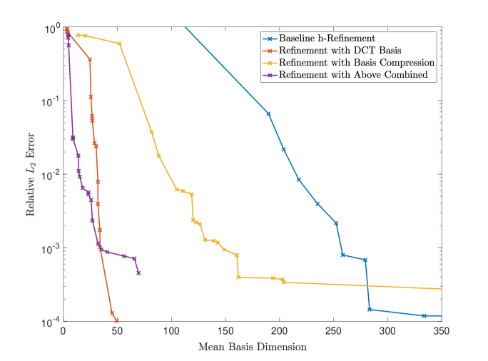
Figure 5: Pareto front comparison for FitzHugh–Nagumo system. This figure contains Pareto fronts computed for four different versions of our method on the FitzHugh–Nagumo example. The method executed with leaf basis $\mathbf{Q}_{\text{K}}$ and no basis compression, shown in blue, is identical to the original $h$-refinement method and serves as a baseline for performance comparison. The other variants correspond to the method executed with leaf basis $\mathbf{Q}_{\text{DCT}}$ and no basis compression, shown in orange; the method performed with leaf basis $\mathbf{Q}_{\text{K}}$ and basis compression, shown in yellow; and the method with $\mathbf{Q}_{\text{DCT}}$ and basis compression, shown in purple. In this case, the ROM executed with the fixed initial basis $\mathbf{\Phi}^{(0)}$ of dimension $3$ yielded $387\%$ error. The proposed method is able to reduce this error to arbitrarily low levels while maintaining reasonable basis dimensions. Furthermore, note that the major contributions of this paper, the ability to specify any arbitrary leaf basis, and the ability to perform basis compression, both lead to very significant performance increases over the original $h$-refinement method.

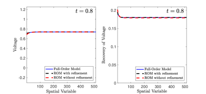
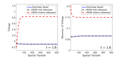
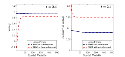
Figure 6: Comparison of FitzHugh-Nagumo Solutions. This figure compares solutions $v(x)$ (Voltage) and $w(x)$ (Recovery of Voltage) to the FitzHugh–Nagumo system in section 9.1 above at four different times $t$. The full-order model solution in shown in blue, while the base reduced-order model we use is shown in dotted red. The base reduced-order model combined with our refinement algorithm is shown in dotted black. In particular, we use a DCT refinement tree with $8$ children, child grouping enabled, a compression frequency of $25$ and a full-order model tolerance of $\varepsilon=0.0005$. The mean basis dimension of our refined ROM is $48$ (for comparison, the problem dimension is $1024$). The dynamics of this FitzHugh–Nagumo System involve bouncing back and forth between two regions in phase space. These bounces (i.e., neural spikes) happen on a very short time scale and are very difficult for the base ROM to capture. Indeed, as we see above, the base ROM is incapable of resolving these spikes and hence remains stuck in one region of phase space for the entirety of the simulation. Our refinement algorithm allows this behavior to be resolved very precisely, with final relative $\ell^{2}$ error of $0.7\%$.

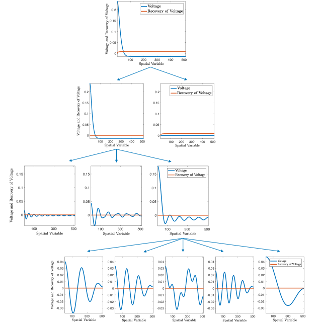
Figure 7: An illustration of the refinement of a ROM basis vector as it is sieved through the refinement tree in the FitzHugh–Nagumo case study above. The degrees of freedom are laid out as described in section 9.1. The first split corresponds to the vector space decomposition $\mathbb{R}^{n}=\mathbb{U}^{(v)}+\mathbb{U}^{(w)}$, decoupling the degrees of freedom corresponding to $v$ and $w$, respectively. After this first refinement, the next two refinements the refinement algorithm performs two band-pass filters to decouple the low frequencies on the degrees of freedom corresponding to $v$. Typically, the solutions to the FitzHugh–Nagumo system in section 9.1 are very smooth on the computational domain, with the exception of at the boundary. Hence, by isolating low frequencies components from the original ROM basis vector, our refined model is able to efficiently represent smooth data, leading to significantly lower average basis dimension than if one had used a refinement tree corresponding to the Kronecker basis. This performance increase is evident in fig. 5.

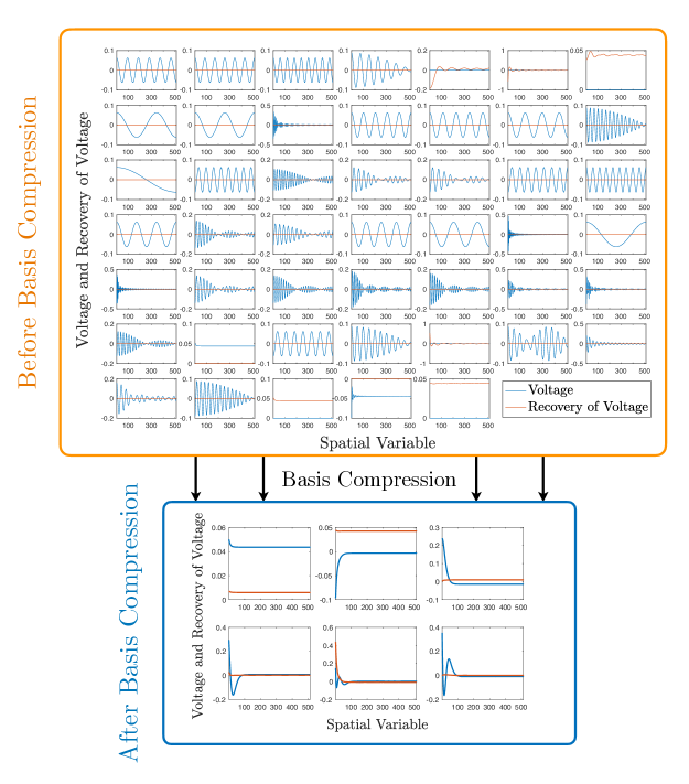
Figure 8: Visualization of basis compression. This figure presents a visualization of our basis compression algorithm on the FitzHugh–Nagumo system in section 9.1. The compression algorithm allows us to reduce the dimension of our refined ROM without losing the ability to represent solution data at previous time steps. In this case, the compression algorithm determines the important fidelity added to the ROM via refinement is concentrated on the left-hand side of the domain, and the remainder of the additional representative power of the refined ROM can be discarded without significantly impacting the ROM’s ability to capture solution data at previous time steps. If the underlying system exhibits some degree of temporal coherence, then this technique can lead to significant reduction in average basis dimension over simply resetting the ROM, as seen in fig. 5.

9.2 Nonlinear transmission line model

The second example we consider corresponds to a nonlinear transmission line model [40], which simulates the behavior of a particular circuit consisting of resistors, capacitors, and diodes and has been used as a benchmark problem for model-reduction techniques. The system consists of a collection of $n=100$ nodes, with the unknowns corresponding to the voltages $v_{1},\ldots,v_{n}$ at each of these nodes such that the state vector is $\boldsymbol{x}=\left[\begin{array}[]{ccc}v_{1}&\ldots&v_{n}\end{array}\right]^{T}$. The dynamics can be expressed as a system of nonlinear ODEs

$$\frac{d\boldsymbol{x}}{dt}=\boldsymbol{f}(\boldsymbol{x})+\mathbf{B}\,u(t)\,,$$ (9.10)

where the velocity $\boldsymbol{f}$ is

$$\boldsymbol{f}:\boldsymbol{x}\mapsto\left[\begin{array}[]{cccccc}-2&1&&&&\\ 1&-2&1&&&\\ &1&\ddots&\ddots&&\\ &&\ddots&-2&1&\\ &&&1&-2&1\\ &&&&1&-2\end{array}\right]\boldsymbol{x}+\left[\begin{array}[]{c}2-\exp(40x_{1})-\exp(40(x_{1}-x_{2}))\\ \exp(40(x_{1}-x_{2}))-\exp(40(x_{2}-x_{3}))\\ \exp(40(x_{2}-x_{3}))-\exp(40(x_{3}-x_{4}))\\ \vdots\\ \exp(40(x_{n-2}-x_{n_{1}}))-\exp(40(x_{n-1}-x_{n}))\\ \exp(40(x_{n-1}-x_{n}))-1\end{array}\right]\,,$$ (9.11)

and the input matrix is $\mathbf{B}\equiv\left[\begin{array}[]{cccc}1&0&\cdots&0\end{array}\right]^{T}$ such that the input current $u(t)$ enters the first node. The initial condition is given by $\left.\boldsymbol{x}\right|_{t=0}=\boldsymbol{0}$. To numerically integrate the governing ODE system in the time interval $\mathbb{T}=[0,10]$, we employ the backward-Euler scheme with a time step size $\Delta t=0.01$.

As in the previous example, we again demonstrate that the proposed method’s ability to consider general refinement mechanisms and perform online basis compression can yield substantial performance improvements over the original $h$-refinement method. Once again, we construct two refinement trees $T_{\text{DCT}}$ and $T_{\text{K}}$ associating with a discrete cosine transform leaf basis and a standard Kronecker leaf basis, respectively.

We consider a predictive scenario wherein training is executed for a training input $u(t)=u_{\text{train}}(t)\vcentcolon=1-{t}/{50}$ and testing is executed for an online input $u(t)=u_{\text{test}}(t)\vcentcolon=1/2(\cos(2\pi t/10)+1)$. We set the initial basis $\mathbf{\Phi}^{(0)}$ to the first $p_{0}=4$ POD vectors of snapshot data $\mathbf{X}\in\mathbb{R}^{n\times q}$ with $q=1000$ collected at the training input.

To generate the trees $T_{\text{DCT}}$ and $T_{\text{K}}$, we use the procedure outlined in section 6, with

$$\begin{split}\mathbf{Q}_{\text{DCT}}&\equiv\mathbf{M}^{(n)}_{\text{DCT}}\,,\\ \mathbf{Q}_{K}&\equiv\mathbf{I}^{(n)}\,,\end{split}$$ (9.12)

where $\mathbf{M}^{(n)}_{\text{DCT}}$ is the $n\times n$ DCT-II matrix and $\mathbf{I}^{(n)}$ is the $n\times n$ identity. We use the snapshot data $\mathbf{X}$ as the input to the tree-construction procedure.

Fig. 9 reports the resulting Pareto fronts, which arise from varying all hyperparameters according to values in table 2. Once again, we observe the new contributions of this work to yield significant performance improvements over the original $h$-refinement method. In particular, using the DCT basis with online basis compression clearly yields the best performance. We note that the ROM with the (fixed) original basis of dimension three yielded 20.2% relative error. Just like in the FighHugh-Nagumo example, we provide another simultaneous printout of the solutions to the FOM, refined ROM, and unrefined ROM in fig. 10. We note again that the unrefined ROM fails to fully resolve the physics of the FOM, but the refined ROM performs quite well.

Hyperparameter	Test Values
Tree Topology: Number of Children ($k$)	$2,4,8,12$
Child Grouping	true, false
Number of Time Steps Between Basis Resets / Compressions ($N_{reset}$)	$10,25,50,75$
Full-Order Model Tolerance ($\varepsilon$)	$0.01,0.005,0.002,0.001,$ $0.0005,0.0002,0.0001,0.00005$
Reduced-Order Model Tolerance ($\varepsilon_{ROM}$)	$10^{-8}$

Table 2: Marginal hyper-parameter choices for Pareto plot shown in fig. 9.

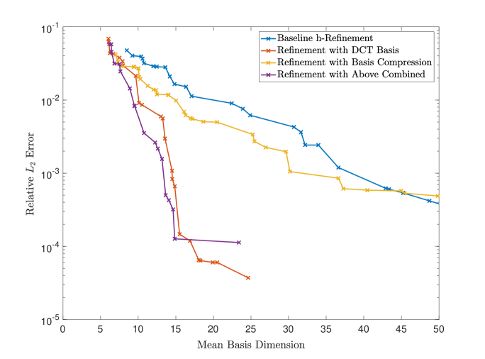
Figure 9: Pareto front comparison for the Nonlinear Transmission Line system. This figure contains Pareto fronts computed for four different versions of our method on the Nonlinear Transmission Line example. The method executed with leaf basis $\mathbf{Q}_{\text{K}}$ and no basis compression, shown in blue, is identical to the original $h$-refinement method and serves as a baseline for performance comparison. The other variants correspond to the method executed the method performed with leaf basis $\mathbf{Q}_{\text{DCT}}$ and no basis compression, shown in orange; the method performed with leaf basis $\mathbf{Q}_{\text{K}}$ and basis compression, shown in yellow; and the method with $\mathbf{Q}_{\text{DCT}}$ and basis compression, shown in purple. In this case, the ROM executed with the fixed initial basis $\mathbf{\Phi}^{(0)}$ of dimension $4$ yielded $20.2\%$ error. Again, the proposed method is able to reduce this error to arbitrarily low levels while maintaining reasonable basis dimensions. Furthermore, note that the major contributions of this paper, the ability to specify any arbitrary leaf basis, and the ability to perform basis compression, both lead to very significant performance increases over the original $h$-refinement method.

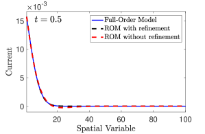
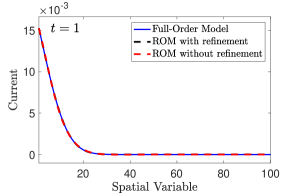
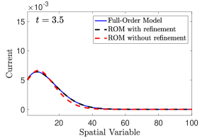
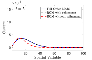
Figure 10: Comparison of Nonlinear Transmission Line Solutions. This figure shows an illustration of the output of our algorithm on the nonlinear transmission line system in section 9.2 at different times $t$. The full-order model solution in shown in blue, while the base reduced-order model we use is shown in dotted red. The base reduced-order model combined with our refinement algorithm is shown in dotted black. In particular, we use a DCT refinement tree with $8$ children, child grouping enabled, a compression frequency of $25$ and a full-order model tolerance of $\varepsilon=0.001$. The mean basis dimension of our refined ROM is $13$ (for comparison, the problem dimension is $100$). The dynamics of this Nonlinear Transmission Line System involves relaxation from a pulse at $t=0$. We note that the base ROM performs well initially, but fails to resolve later times correctly. On the other hand, our refinement algorithm allows this behavior to be resolved, with final relative $\ell^{2}$ error of $1.9\%$.

10 Conclusions

This work has proposed an online adaptive basis refinement and compression method for reduced-order models. The principal new contributions of the method include:

1. A mathematical framework, presented in sections 3, 5, and 6, that generalizes the original ROM $h$-refinement method [12], as it enables a general basis-refinement mechanism based on recursive vector-space decompositions. This allows for custom tailoring of the ROM refinement mechanism to the particular problem, which we have demonstrated can significantly improve performance over the original approach.

2. A novel online basis-compression algorithm, presented in section 7, which controls the dimension of the refined basis online while ensuring an $n$-independent operation count. We have demonstrated that this aspect of the method enables additional substantial performance improvements over the original approach.

The proposed approach distinguishes itself from existing approaches for online ROM adaptivity in that it avoids any FOM solves, yet it also ensures monotone convergence to the full-order model, as proved in theorems 5.4 and 5.5.

Future research directions include integrating hyper-reduction techniques such as collocation, empirical interpolation, or gappy POD into the proposed framework. This would entail adaptively adding/removing residual sampling points to maintain well-posedness of the refined-ROM system; one challenge here involves ensuring the sampling pattern is ‘compatible’ with the refined basis, so that one does not run into the scenario where, for example, many sample points fall outside the supports of refined basis vectors. Another direction for investigation entails devising approaches to reduce the storage requirements for leaf vector spaces with global support, either by using an on-the-fly computation approach (as we employ to compute the metric $\mathbf{V}^{T}\mathbf{V}$) or perhaps via a sampling approach. Finally, future work entails applying the proposed method to a truly large-scale industrial problem.

Appendix A Modified splitting algorithm

In this appendix, we give a pseudocode integration of the conditioning technique we presented in section 5.4 into the refinement algorithm 3. To perform this integration, we must maintain a list $\mathcal{I}\subset\bigsqcup_{i}\mathcal{F}_{i}$ of inactive vertices in the frontiers $\mathcal{F}_{1},...,\mathcal{F}_{p_{0}}$. After refinement, whenever a vertex is detected by the ill-conditioning check in 5.4, we place it into the list $\mathcal{I}$. Afterwards, during the frontier refinement algorithm, specifically during the computation of the full refinement $\bar{\mathcal{F}}^{h}$ of the global frontier $\bar{\mathcal{F}}^{H}\equiv\bigsqcup_{i}\mathcal{F}_{i}$ we deliberately exclude all of the vertices in $\mathcal{I}$ from taking part in refinement. Furthermore, we also implement basis vector rescaling, which maintains a scale factor for every active frontier element in $\bigsqcup_{i}\mathcal{F}_{i}\setminus\mathcal{I}$ , as described in section 5.4.

Below, in algorithms 13, 14, 15, we give the modified versions of the algorithms 1, 2, 3 respectively as described in section 5.4. Note that in algorithm 15, the implementation of HandleFullInactiveVertices is deferred to the user. This routine is triggered when all available refinement options have been systematically deactivated by the conditioning technique. If the value of the cutoff $\epsilon_{\text{QR}}$ used for the conditioning technique is too high, it is possible that we may disable all available refinement options before we converge to a solution that is within the desired tolerance. In order to address this, there are a number of things the user can do to reactivate vertices which have been deactivated if this corner case is reached. two possibilities include:

1. Simply resetting $\mathcal{I}$ to empty and halving the value of $\epsilon_{\text{QR}}$.

2. Performing a column-pivoted QR decomposition of $\left[\begin{array}[]{ccc}P_{\mathcal{F}_{1}}\left[\boldsymbol{\phi}_{1}\right]&\cdots&P_{\mathcal{F}_{p_{0}}}\left[\boldsymbol{\phi}_{p_{0}}\right]\end{array}\right]$ to determine which elements of $\mathcal{I}$ to reactivate. Optionally, one can modify $\epsilon_{\text{QR}}$ by examining the diagonal values of the above QR decomposition.

The specific implementation may depend on the use-case, and hence is left up to the user.

Algorithm 13 Modified computation of Error Indicators

Input: The current coarse basis $\mathbf{V}^{H}_{*}$, the current frontiers $\mathcal{F}_{1},\ldots,\mathcal{F}_{p_{0}}$, the set of inactive vertices $\mathcal{I}$.
      Output: The fine error indicators $\boldsymbol{\delta}^{h}$.

1:procedure ComputeErrorIndicators($\mathbf{V}^{H}_{*}$, $\mathcal{F}_{1},\ldots,\mathcal{F}_{p_{0}},\mathcal{I}$)

2:     $\bar{\mathcal{F}}^{H}\leftarrow\left(\bigsqcup_{i}\mathcal{F}_{i}\right)\setminus\mathcal{I}$

3:     $\bar{\mathcal{F}}^{h}\leftarrow\bigsqcup_{i}\left(\bigcup_{\mathbb{U}\in\mathcal{F}_{i}\setminus\mathcal{I}}R_{T}\left(\mathbb{U}\right)\right)$ $\triangleright$ To compute the refined global frontier $\bar{\mathcal{F}}^{h}$, we refine all spaces in $\bar{\mathcal{F}}^{H}$ except those marked as inactive.

4:     $\mathbf{I}^{h}_{H}\leftarrow\textsc{ComputeProlongationOperator}\left(\bar{\mathcal{F}}^{H},\bar{\mathcal{F}}^{h}\right)$ $\triangleright$ Compute prolongation operator using Eq. (5.11)

5:      $\hat{\mathbf{y}}^{H}\leftarrow\left[(\mathbf{V}^{H}_{*})^{T}\frac{\partial\boldsymbol{r}}{\partial\boldsymbol{x}}(\mathbf{V}^{H}_{*}\hat{\boldsymbol{x}}^{H})^{T}\mathbf{V}^{H}_{*}\right]^{-T}\left[(\mathbf{V}^{H}_{*})^{T}\frac{\partial g}{\partial\boldsymbol{x}}\left(\mathbf{V}^{H}_{*}\hat{\boldsymbol{x}}^{H}\right)^{T}\right]$ $\triangleright$ Compute the coarse adjoint using Eq. (5.23)

6:     $\hat{\mathbf{y}}^{h}_{H}\leftarrow\mathbf{I}^{h}_{H}\hat{\mathbf{y}}^{H}$ $\triangleright$ Prolongate coarse adjoint to fine coordinate space.

7:     $\boldsymbol{\delta}^{h}\leftarrow\boldsymbol{0}\in\mathbb{R}^{\bar{\mathcal{F}}^{h}}$

8:     for $\mathbb{W}\in\bar{\mathcal{F}}^{h}\setminus\mathcal{L}$ do

9:         $\boldsymbol{\delta}^{h}_{\mathbb{W}}\leftarrow\left|\left[\hat{\mathbf{y}}^{h}_{H}\right]_{\mathbb{W}}\left(\boldsymbol{v}_{\mathbb{W}}^{h}\right)^{T}\boldsymbol{r}\left(\mathbf{V}^{H}\hat{\boldsymbol{x}}^{H}\right)\right|$$\triangleright$ Compute the error indicators using Eq. (5.26)

10:     end for

11:     return $\boldsymbol{\delta}^{h}$

12:end procedure

Algorithm 14 Modified computation of Refined Frontiers

Input: The $\mathbb{R}^{n}$-refinement tree $T$, the fine error indicators $\boldsymbol{\delta}^{h}$, the current frontiers $\mathcal{F}_{1},\ldots,\mathcal{F}_{p_{0}}$, the set of inactive vertices $\mathcal{I}$.
      Output: A new set of frontiers $\mathcal{F}_{1}^{\prime},\ldots,\mathcal{F}_{p_{0}}^{\prime}$ refined according to the input error indicators.

1:procedure RefineFrontiers($T,\boldsymbol{\delta}^{h},\mathcal{F}_{1},\ldots,\mathcal{F}_{p_{0}}$)

2:     $\bar{\mathcal{F}}^{H}\leftarrow\left(\bigsqcup_{i}\mathcal{F}_{i}\right)\setminus\mathcal{I}$

3:     $\bar{\mathcal{F}}^{h}\leftarrow\bigsqcup_{i}\left(\bigcup_{\mathbb{U}\in\mathcal{F}_{i}\setminus\mathcal{I}}R_{T}\left(\mathbb{U}\right)\right)$ $\triangleright$ To compute the refined global frontier $\bar{\mathcal{F}}^{h}$, we refine all spaces in $\bar{\mathcal{F}}^{H}$.

4:     $\psi\leftarrow\textsc{GetGlobalAncestorMap}\left(\bar{\mathcal{F}}^{h},\bar{\mathcal{F}}^{H}\right)$ $\triangleright$ Compute the map in Eq. (5.10) sending every space to its ancestor.

5:     $\mathbf{I}^{h}_{H}\leftarrow\textsc{ComputeProlongationOperator}\left(\bar{\mathcal{F}}^{H},\bar{\mathcal{F}}^{h}\right)$ $\triangleright$ Compute prolongation operator using Eq. (5.11).

6:     $\boldsymbol{\delta}^{H}=\boldsymbol{\delta}^{h}\mathbf{I}^{h}_{H}$ $\triangleright$ Compute coarse error indicators using Eq. (5.28).

7:     $\eta\leftarrow\frac{1}{|\bar{\mathcal{F}}^{H}|}\sum_{\mathbb{U}\in\bar{\mathcal{F}}^{H}}\boldsymbol{\delta}^{H}_{\mathbb{U}}$ $\triangleright$ Compute the average of the coarse error indicators.

8:     $S\leftarrow\{\mathbb{U}\in\bar{\mathcal{F}}^{H}\mid\boldsymbol{\delta}^{H}_{\mathbb{U}}\geq\eta\}$ $\triangleright$ Select the spaces in $\bar{\mathcal{F}}^{H}$ whose coarse error indicator is greater than average.

9:     for $i\in\mathbb{N}(p_{0})$ do $\triangleright$ For each frontier $\mathcal{F}_{i}$

10:         $S_{i}\leftarrow\mathcal{F}_{i}\cap S$ $\triangleright$ Extract the elements of $S$ that came from $\mathcal{F}_{i}$.

11:         $\mathcal{F}_{i}^{\prime}\leftarrow R_{T}\left(\mathcal{F};S_{i}\right)$ $\triangleright$ Refine the frontier $\mathcal{F}_{i}$ at these spaces.

12:     end for

13:     return $(\mathcal{F}_{1}^{\prime},\ldots,\mathcal{F}_{p_{0}}^{\prime})$ $\triangleright$ Return the refined frontiers.

14:end procedure

Algorithm 15 Refinement Algorithm

Input: $\mathbb{R}^{n}$-refinement tree $T$, initial basis $\mathbf{\Phi}$, current frontiers $\mathcal{F}_{1},\ldots,\mathcal{F}_{p_{0}}$, reference solution $\bar{\boldsymbol{x}}$, residual function $\boldsymbol{r}$, ROM-residual tolerance $\varepsilon_{ROM}$, and FOM-residual tolerance $\varepsilon$, the set of inactive vertices $\mathcal{I}$ (initially empty), a cutoff $\epsilon_{\text{QR}}$ for the conditioning technique.
      Output: A new set of frontiers $\mathcal{F}_{1}^{\prime},\ldots,\mathcal{F}_{p_{0}}^{\prime}$ refined according to the input error indicators, the new set of inactive vertices $\mathcal{I}^{\prime}$.

1:procedure SolveModel($T,\mathbf{\Phi},\mathcal{F}_{1},\ldots,\mathcal{F}_{p_{0}},\bar{\boldsymbol{x}},\varepsilon_{ROM},\varepsilon,\mathcal{I},\epsilon_{\text{QR}}$)

2:     while True do $\triangleright$ Refine the basis until the specified full-order tolerance is met.

3:         if $\left(\bigsqcup_{i}\mathcal{F}_{i}\right)\setminus\mathcal{L}\subset\mathcal{I}$ then $\triangleright$ If there are no viable refinement options available because all of them have been deactivated.

4:              HandleFullInactiveVertices $\triangleright$ Reactivate inactive vertices, specific implementation is left to the user. See above for suggestions.

5:         end if

6:          $\mathbf{V}^{H}\leftarrow\left[\begin{array}[]{ccc}P_{\mathcal{F}_{1}}\left[\boldsymbol{\phi}_{1}\right]&\cdots&P_{\mathcal{F}_{p_{0}}}\left[\boldsymbol{\phi}_{p_{0}}\right]\end{array}\right]$ $\triangleright$ Retrieve the current coarse model basis.

7:         $\mathbf{V}^{H}_{*}\leftarrow\mathbf{V}^{H}_{:,\left(\bigsqcup_{i}\mathcal{F}_{i}\right)\setminus\mathcal{I}}$ $\triangleright$ Remove columns of $\mathbf{V}^{H}$ which correspond to vertices in $\mathcal{I}$

8:         $\sigma^{H}_{*}\leftarrow\left\{1/\|(\mathbf{V}^{H}_{*})_{:,\mathbb{U}}\|_{2}\mid\mathbb{U}\in\left(\bigsqcup_{i}\mathcal{F}_{i}\right)\setminus\mathcal{I}\right\}$ $\triangleright$ Get inverse norms of all columns in $\mathbf{V}^{H}$

9:         $\mathbf{\Sigma}^{H}_{*}\leftarrow\text{diag}(\sigma^{H}_{*})$

10:         $\mathbf{V}^{H}_{*}\leftarrow\mathbf{V}^{H}\mathbf{\Sigma}_{*}$ $\triangleright$ Rescale the columns of $\mathbf{V}^{H}$

11:         $\hat{\boldsymbol{x}}\leftarrow\textsc{SolveROM}(\boldsymbol{r},\mathbf{V}^{H}_{*},\bar{\boldsymbol{x}},\varepsilon_{ROM})$ $\triangleright$ Solve the system $(\mathbf{V}^{H})^{T}\boldsymbol{r}\left(\bar{\boldsymbol{x}}+\mathbf{V}^{H}_{*}\hat{\boldsymbol{x}}\right)=0$ from Eq. (2.5).

12:         $\boldsymbol{x}\leftarrow\mathbf{V}^{H}_{*}\hat{\boldsymbol{x}}$ $\triangleright$ Lift the result to the full-order model.

13:         if $\|\boldsymbol{r}(\boldsymbol{x})\|_{2}<\varepsilon$ then $\triangleright$ Check if the full-order residual is within the specified tolerance.

14:              break $\triangleright$ If the specified tolerance is satisfied, stop refinement.

15:         end if

16:          $\boldsymbol{\delta}^{h}\leftarrow\textsc{ComputeErrorIndicators}(\mathbf{V}^{H}_{*},\mathcal{F}_{1},\ldots,\mathcal{F}_{p_{0}})$ $\triangleright$ Compute the error indicators in Eq. (5.26).

17:          $(\mathcal{F}_{1},\ldots,\mathcal{F}_{p_{0}})\leftarrow\textsc{RefineFrontiers}(T,\boldsymbol{\delta}^{h},\mathcal{F}_{1},\ldots,\mathcal{F}_{p_{0}})$ $\triangleright$ Use error indicators to selectively refine frontiers.

18:          $\mathbf{V}^{h}\leftarrow\left[\begin{array}[]{ccc}P_{\mathcal{F}_{1}}\left[\boldsymbol{\phi}_{1}\right]&\cdots&P_{\mathcal{F}_{p_{0}}}\left[\boldsymbol{\phi}_{p_{0}}\right]\end{array}\right]$ $\triangleright$ Retrieve the current refined model basis.

19:         $\mathbf{V}^{h}\leftarrow\mathbf{V}^{h}_{:,\left(\bigsqcup_{i}\mathcal{F}_{i}\right)\setminus\mathcal{I}}$ $\triangleright$ Remove columns of $\mathbf{V}^{h}$ which correspond to vertices in $\mathcal{I}$

20:         $\sigma^{h}\leftarrow\left\{1/\|\mathbf{V}^{h}_{:,\mathbb{U}}\|_{2}\mid\mathbb{U}\in\left(\bigsqcup_{i}\mathcal{F}_{i}\right)\setminus\mathcal{I}\right\}$ $\triangleright$ Get inverse norms of all columns in $\mathbf{V}^{h}$

21:         $\mathbf{\Sigma}^{h}\leftarrow\text{diag}(\sigma^{h})$

22:         $\mathbf{V}^{h}\leftarrow\mathbf{V}^{h}\mathbf{\Sigma}^{h}$ $\triangleright$ Rescale the columns of $\mathbf{V}^{h}$

23:         $(\mathbf{Q},\mathbf{R},\pi)\leftarrow\textsc{CPQR}(\mathbf{V}^{h})$ $\triangleright$ Take column-pivoted QR factorization of $\mathbf{V}^{h}$; $\pi$ denotes the resulting column permutation.

24:         $k\leftarrow\max_{i}\{i\mid\mathbf{R}_{ii}\geq\epsilon_{\text{QR}}\}$ $\triangleright$ Find the selection cutoff $k$ for the columns of $\mathbf{V}^{h}$.

25:         $\mathcal{I}_{\text{new}}\leftarrow\pi_{k+1:\text{end}}$ $\triangleright$ The spaces corresponding to the columns which occur after the cutoff $k$ must now be marked as inactive.

26:         $\mathcal{I}\leftarrow\mathcal{I}\cup\mathcal{I}_{\text{new}}$$\triangleright$ Add the above spaces to the set of inactive spaces.

27:     end while

28:     return $(\mathcal{F}_{1},\ldots,\mathcal{F}_{p_{0}},\hat{\boldsymbol{x}},\mathcal{I})$.

29:end procedure

Appendix B Child grouping

To better curtail the ROM dimension increase of a refinement, we may not want to split a parent node completely into all of its children, but rather into groups of children, as was done in the previous reduced-order model $h$-refinement paper [12]. These considerations motivate the definition of a generalized frontier,

Definition B.1 (generalized frontier).

A generalized frontier $\tilde{\mathcal{F}}$ (i.e., a frontier with child grouping) of a refinement tree $T$ is an orthogonal decomposition of $\mathbb{R}^{n}$ such that there exists a frontier $\mathcal{F}$ of $T$ satisfying

$$\mathcal{F}\preceq\tilde{\mathcal{F}}\,,$$ (B.1)

with the property that the ancestor map $\psi:\mathcal{F}\longrightarrow\tilde{\mathcal{F}}$ satisfies

$$\psi(\mathbb{U})\subset P_{T}(\mathbb{U}),\qquad\forall\mathbb{U}\in\mathcal{F}\,,$$ (B.2)

where $P_{T}(\mathbb{U})$ denotes the parent of $\mathbb{U}$ in $T$.

The concept of a generalized frontier provides a useful range of resolutions between the coarse frontier $\mathcal{F}$ and the refinement $\mathcal{F}^{+}$. In practice, a generalized frontier $\tilde{\mathcal{F}}$ can be represented on a computer by storing the frontier $\mathcal{F}$ in Eq. (B.1) together with the induced ancestor map $\psi:\mathcal{F}\longrightarrow\tilde{\mathcal{F}}$. Note that this representation $(\mathcal{F},\psi)$ of a generalized frontier may not be unique without additional constraints, but every generalized frontier can be represented as such. To guarantee uniqueness of the frontier $\mathcal{F}$, we use the convention that

$$(\mathcal{F}\cap\tilde{\mathcal{F}})\setminus\mathcal{L}=\emptyset\,.$$ (B.3)

We give this $\mathcal{F}$ above a definition:

Definition B.2 (Full refinement of a generalized frontier).

The full refinement of a generalized frontier $\tilde{\mathcal{F}}$ is any frontier $\mathcal{F}$ which satisfies Eqs. (B.1), (B.2), and (B.3). We denote the full refinement of a generalized frontier $\tilde{\mathcal{F}}$ as $(\tilde{\mathcal{F}})^{+}$.

Proposition B.1 (Uniqueness of full refinements of generalized frontiers).

The full refinement of a generalized frontier exists and is unique.

This definition now allows for straightforward generalization of the refinement algorithms 1 and 3 to generalized frontiers by simply replacing the frontiers $\mathcal{F}_{1},...,\mathcal{F}_{k}$ with generalized frontiers $\tilde{\mathcal{F}}_{1},...,\tilde{\mathcal{F}}_{k}$. On the other hand, to make use of the additional freedom that generalized frontiers give us in performing refinement, we modify algorithm 2, which actually performs the frontier refinement. This modification is a direct extension of the child grouping mechanism from the original ROM $h$-refinement paper [12].

To begin, note that $\tilde{\mathcal{F}}$ can be thought of as a special grouping of the spaces in $(\tilde{\mathcal{F}})^{+}$. From Eq. (B.1) above, every space in $\tilde{\mathcal{F}}$ is a sum of a group of spaces in $(\tilde{\mathcal{F}})^{+}$, with the property, imparted from Eq. (B.2), that groupped spaces must have the same parent in the tree $T$. The generalized frontier structure is therefore directly analogous to child grouping from ROM $h$-refinement.

Just like our refinement algorithm 3 does not necessarily refine a frontier $\mathcal{F}$ to its full refinement $\mathcal{F}^{+}$, we also do not necessarily have to split the spaces $\mathbb{U}\in\tilde{\mathcal{F}}$ we select for refinement into all of their individual consituents $\psi^{-1}(\mathbb{U})$ in $(\tilde{\mathcal{F}})^{+}$. Instead, we opt to use the dual-weighted error residual indicators $\boldsymbol{\delta}^{h}$ in Eq. (5.26) to determine a more conservative refinement.

This is done as follows: suppose we select $\mathbb{U}\in\tilde{\mathcal{F}}$ for refinement, i.e., the coarse error indicator $\boldsymbol{\delta}^{H}_{\mathbb{U}}$ is larger than the average of the coarse error indicators for the spaces in $\tilde{\mathcal{F}}$. The coarse error indicator can then be decomposed in terms of the fine error indicators for constituent spaces of $\mathbb{U}$ (see Eq. (5.27)),

$$\boldsymbol{\delta}^{H}_{\mathbb{U}}=\sum_{\mathbb{W}\in\psi^{-1}(\mathbb{U})}\boldsymbol{\delta}^{h}_{\mathbb{W}}\,.$$ (B.4)

Since these error indicators give us a rough estimate of the reduction in error achieved by refining fully to a specific vector space in $\psi^{-1}(\mathbb{U})$, one principled way of refining $\mathbb{U}$ into subgroups $G_{i}\subset\psi^{-1}(\mathbb{U})$ of spaces in $\psi^{-1}(\mathbb{U})$ would be to split $\psi^{-1}(\mathbb{U})$ in such a way that the subgroups $G_{i}$ have roughly equal cumulative error indicators $\sum_{\mathbb{W}\in G_{i}}\boldsymbol{\delta}^{h}_{\mathbb{W}}$. More precisely, given some splitting factor $0<\alpha<1$, we would like to find a decomposition of $\psi^{-1}(\mathbb{U})$ into a minimal number of disjoint subgroups $G_{i}$ with the property that each subgroup has a cummulative error that is at most a fraction $\alpha$ of the total cummulative error $\boldsymbol{\delta}^{H}_{\mathbb{U}}$ of $\psi^{-1}(\mathbb{U})$, i.e.,

$$\sum_{\mathbb{W}\in G_{i}}\boldsymbol{\delta}^{h}_{\mathbb{W}}\leq\alpha\boldsymbol{\delta}^{H}_{\mathbb{U}}\,.$$ (B.5)

This is the well-known bin-packing problem, which is $\mathcal{NP}$-hard. We use the inexpensive and easily implemented greedy first-fit algorithm to generate the sets $G_{i}$. Greedy first-fit achieves the optimal number of bins within a factor of $2$, although there are other common approximation algorithms one may use if so inclined. Note that smaller values of $\alpha$ correspond to more aggressive splitting. Once the sets $G_{i}$ have been calculated, we define the corresponding spaces $\mathbb{G}_{i}$ as

$$\mathbb{G}_{i}\equiv\sum_{\mathbb{W}\in G_{i}}\mathbb{W}\,.$$ (B.6)

From the properties of the ancestor map $\psi$, it is easy to see that these spaces form an orthogonal decomposition $\mathcal{U}_{\mathbb{U}}=\{\mathbb{G}_{i}\}_{i}$ of the parent space $\mathbb{U}$. Hence, if $\mathbb{U}_{1},...,\mathbb{U}_{b}\in\tilde{\mathcal{F}}$ are marked for refinement, and $\mathcal{U}_{\mathbb{U}_{1}},...,\mathcal{U}_{\mathbb{U}_{b}}$ are the corresponding decompositions of these spaces computed with the greedy binning strategy above, then our refinement step becomes

$$\tilde{\mathcal{F}}^{\prime}\leftarrow R\left(\tilde{\mathcal{F}};\mathcal{U}_{\mathbb{U}_{1}},\ldots,\mathcal{U}_{\mathbb{U}_{b}}\right)\,.$$ (B.7)

Note $\tilde{\mathcal{F}}^{\prime}$ is an orthogonal decomposition by remark (5.3) and that the full refinement $(\tilde{\mathcal{F}})^{+}$ of $\tilde{\mathcal{F}}$ serves as the frontier $\mathcal{F}$ in Eqs. (B.1) and (B.2) for the orthogonal decomposition $\tilde{\mathcal{F}}^{\prime}$. This makes $\tilde{\mathcal{F}}^{\prime}$ a generalized frontier. The pseudocode for computing the refinement of $\tilde{\mathcal{F}}$ is given in algorithm 16.

Algorithm 16 Computation of Refined Generalized Frontiers

Input: The $\mathbb{R}^{n}$-refinement tree $T$, the fine error indicators $\boldsymbol{\delta}^{h}$, the current generalized frontiers $\tilde{\mathcal{F}}_{1},\ldots,\tilde{\mathcal{F}}_{p_{0}}$.
      Output: A new set of generalized frontiers $\tilde{\mathcal{F}}_{1}^{\prime},\ldots,\tilde{\mathcal{F}}_{p_{0}}^{\prime}$ refined according to the input error indicators.

1:procedure RefineFrontiers($T,\boldsymbol{\delta}^{h},\tilde{\mathcal{F}}_{1},\ldots,\tilde{\mathcal{F}}_{p_{0}}$)

2:     $\bar{\mathcal{F}}^{H}\leftarrow\bigsqcup_{i}\tilde{\mathcal{F}}_{i}$

3:     $\bar{\mathcal{F}}^{h}\leftarrow\bigsqcup_{i}\tilde{\mathcal{F}}^{+}_{i}$

4:     $\psi\leftarrow\textsc{GetGlobalAncestorMap}\left(\bar{\mathcal{F}}^{h},\bar{\mathcal{F}}^{H}\right)$ $\triangleright$ Compute the map in Eq. (5.10) sending every space to its ancestor.

5:     $\mathbf{I}^{h}_{H}\leftarrow\textsc{ComputeProlongationOperator}\left(\bar{\mathcal{F}}^{H},\bar{\mathcal{F}}^{h}\right)$ $\triangleright$ Compute prolongation operator using Eq. (5.11).

6:     $\boldsymbol{\delta}^{H}=\boldsymbol{\delta}^{h}\mathbf{I}^{h}_{H}$ $\triangleright$ Compute coarse error indicators using Eq. (5.28).

7:     $\eta\leftarrow\frac{1}{|\bar{\mathcal{F}}^{H}|}\sum_{\mathbb{U}\in\bar{\mathcal{F}}^{H}}\boldsymbol{\delta}^{H}_{\mathbb{U}}$ $\triangleright$ Compute the average of the coarse error indicators.

8:     $S\leftarrow\{\mathbb{U}\in\bar{\mathcal{F}}^{H}\mid\boldsymbol{\delta}^{H}_{\mathbb{U}}\geq\eta\}$ $\triangleright$ Select the spaces in $\bar{\mathcal{F}}^{H}$ whose coarse error indicator is greater than average.

9:     for $i\in\mathbb{N}(p_{0})$ do $\triangleright$ For each frontier $\mathcal{F}_{i}$

10:         $S_{i}\leftarrow\mathcal{F}_{i}\cap S$ $\triangleright$ Extract the elements of $S$ that came from $\mathcal{F}_{i}$.

11:         $\tilde{\mathcal{F}}_{i}^{\prime}\leftarrow\tilde{\mathcal{F}}_{i}$

12:         for $\mathbb{U}\in S_{i}$ do $\triangleright$ For each space $\mathbb{U}$ to be refined.

13:              $\{G_{1},...,G_{b}\}\leftarrow\textsc{GreedyBinPacking}(\boldsymbol{\delta}^{h}_{\psi^{-1}(\mathbb{U})},\alpha\boldsymbol{\delta}^{H}_{\mathbb{U}})$ $\triangleright$ Perform first-fit algorithm with item sizes $\boldsymbol{\delta}^{h}_{\psi^{-1}(\mathbb{U})}$ and bin size $\alpha\boldsymbol{\delta}^{H}_{\mathbb{U}}$. $G_{1},...,G_{b}$ are the resulting bin contents.

14:              for $j\in\mathbb{N}(b)$ do

15:                  $\mathbb{G}_{j}\leftarrow\sum_{\mathbb{W}\in G_{j}}\mathbb{W}$ $\triangleright$ Compute subspaces corresponding to bin contents.

16:              end for

17:              $\mathcal{U}_{\mathbb{U}}\leftarrow\{\mathbb{G}_{1},...,\mathbb{G}_{b}\}$ $\triangleright$ Construct the orthogonal decomposition of $\mathbb{U}$.

18:              $\tilde{\mathcal{F}}_{i}^{\prime}\leftarrow R\left(\tilde{\mathcal{F}}_{i}^{\prime};\mathcal{U}_{\mathbb{U}}\right)$ $\triangleright$ Split the space $\mathbb{U}$ on $\tilde{\mathcal{F}}$ by using the decomposition $\mathcal{U}_{\mathbb{U}}$.

19:         end for

20:     end for

21:     return $(\tilde{\mathcal{F}}_{1}^{\prime},\ldots,\tilde{\mathcal{F}}_{p_{0}}^{\prime})$ $\triangleright$ Return the refined frontiers.

22:end procedure

Appendix C Proofs of propositions

See 3.1

Proof.

If $\mathbb{W}$ is a descendant of $\mathbb{U}$, then recursive application of the property (2) immediately gives that $\mathbb{W}\subset\mathbb{U}$. Conversely, consider the case where $\mathbb{W}\subset\mathbb{U}$. Let $\mathbb{A}\in\mathcal{V}$ be the first common ancestor of $\mathbb{W}$ and $\mathbb{U}$. If $\mathbb{A}=\mathbb{U}$, then the desired result holds automatically. If $\mathbb{A}=\mathbb{W}$, then the forward direction implies that $\mathbb{U}\subset\mathbb{W}$ and thus $\mathbb{U}=\mathbb{W}$ and the desired result holds. Otherwise, suppose $\mathbb{A}\neq\mathbb{W}$ and $\mathbb{A}\neq\mathbb{U}$. Because $\mathbb{A}$ is the first common ancestor of $\mathbb{W}$ and $\mathbb{U}$, $\mathbb{W}$ and $\mathbb{U}$ must be descendant from different children $\mathbb{W}^{\prime}$ and $\mathbb{U}^{\prime}$ of $\mathbb{A}$ respectively. Property (3) implies $\mathbb{W}^{\prime}\perp\mathbb{U}^{\prime}$ and the forward direction of the proof implies that $\mathbb{W}\subset\mathbb{W}^{\prime}$ and $\mathbb{U}\subset\mathbb{U}^{\prime}$. Hence, $\mathbb{W}\perp\mathbb{U}$. Furthermore, since every vertex in the tree has a leaf as an ancestor, the forward direction of the proof combined with property (4) implies that all spaces in $\mathcal{V}$ have dimension at least $1$. This fact, combined with $\mathbb{W}\perp\mathbb{U}$ and the assumption $\mathbb{W}\subset\mathbb{U}$ gives a contradiction, proving the backward direction. ∎

See 3.2

Proof.

For the forward direction, if the assumption holds, then the first common ancestor of $\mathbb{U}$ and $\mathbb{W}$ is neither $\mathbb{U}$ nor $\mathbb{W}$. The desired result was now proved as part of the proof of proposition (3.1). For the backward direction, since all spaces in $\mathcal{V}$ have at least dimension $1$, so $\mathbb{W}\perp\mathbb{U}$ implies that neither $\mathbb{W}$ nor $\mathbb{U}$ is a subset of the other. The desired result follows from proposition (3.1). ∎

See 3.3

Proof.

Suppose $\mathcal{F}\subset\mathcal{V}$ is a frontier and suppose for contradiction that there is a leaf $\mathbb{L}$ that is not descendant from any space in $\mathcal{F}$. Since $\mathbb{L}$ is a leaf, this means that $\mathbb{L}$ is incomparable with every element in $\mathcal{F}$, which by (3.1.1) means that $\mathbb{L}$ is orthogonal to every space in $\mathcal{F}$. Hence, $\mathcal{F}$ cannot be a decomposition of $\mathbb{V}$.

Conversely, suppose $\mathcal{F}\subset\mathcal{V}$ is a set of vertices such that every leaf in $\mathbb{L}$ is descendant from exactly one element in $\mathcal{F}$. For each $\mathbb{U}_{i}\in\mathcal{F}$ we denote $\mathbb{L}_{ij}$ as the leaf spaces descendant from $\mathbb{U}_{i}$. Recursive application of properties (1) and (2) of a refinement tree tells us that

$$\mathbb{U}_{i}=\sum_{j}\mathbb{L}_{ij}\,.$$ (C.1)

Therefore, since $\mathbb{U}_{i}$ is incomparable with all $\mathbb{L}_{rj}$ such that $r\neq i$, it follows that $\mathbb{U}_{i}\perp\mathbb{U}_{r}$ for $i\neq r$. Furthermore, since the leaf spaces $\mathbb{L}_{ij}$ sum to $\mathbb{V}$, the spaces $\mathbb{U}_{i}$ must also sum to $\mathbb{V}$. Hence, $\mathcal{F}$ is an orthogonal decomposition of $\mathbb{V}$. ∎

See 3.4

Proof.

The existence of such a map is trivial, it follows from the definition of the partial order $\preceq$. The uniqueness of this map follows from the fact that the elements of $\mathcal{F}_{2}$ must be orthogonal, and hence $\mathbb{W}\in\mathcal{F}_{1}$ can be a subspace of at most one of the spaces in $\mathcal{F}_{2}$. To prove Eq. (3.22), note that, by the above, we must always have $\sum_{\mathbb{W}\in\psi^{-1}(\mathbb{U})}\mathbb{W}\subset\mathbb{U}$. So, suppose for contradiction that $\sum_{\mathbb{W}\in\psi^{-1}(\mathbb{U})}\mathbb{W}\subsetneq\mathbb{U}$. Consider the space

$$\mathbb{W}^{\prime}=\left(\sum_{\mathbb{W}\in\psi^{-1}(\mathbb{U})}\mathbb{W}\right)^{\perp}\cap\mathbb{U}\,.$$ (C.2)

This space cannot be trivial – by assumption, there exists a nonzero $v\in\mathbb{U}\setminus\sum_{\mathbb{W}\in\psi^{-1}(\mathbb{U})}\mathbb{W}$ and projecting out the space $\sum_{\mathbb{W}\in\psi^{-1}(\mathbb{U})}\mathbb{W}$ yields a nonzero vector both in $\mathbb{U}$ and in $\left(\sum_{\mathbb{W}\in\psi^{-1}(\mathbb{U})}\mathbb{W}\right)^{\perp}$. Furthermore, $\mathbb{W}^{\prime}\perp\mathbb{W}$ for $\mathbb{W}\in\psi^{-1}(\mathbb{U})$ by construction, and $\mathbb{W}^{\prime}\perp\mathbb{W}$ for all $\mathbb{W}\in\mathcal{U}_{1}$ such that $\psi(\mathbb{W})\neq\mathbb{U}$ since $\mathbb{W}\subset\psi(\mathbb{W})$, $\psi(\mathbb{W})\perp\mathbb{U}$, and $\mathbb{W}^{\prime}\subset\mathbb{U}$. Therefore, there exists a nonzero vector in $\mathbb{W}^{\prime}$ that is not contained in $\sum_{\mathbb{W}\in\mathcal{U}_{1}}\mathbb{W}$ and hence $\mathcal{U}_{1}$ cannot be an orthogonal decomposition of $\mathbb{V}$, a contradiction. ∎

See 7.1

Proof.

To begin, we prove that the constituents of $\bigwedge_{i}\mathcal{F}_{i}$ are orthogonal to one another. Let $\mathbb{W}\neq\mathbb{W}^{\prime}$ be elements of $\bigwedge_{i}\mathcal{F}_{i}$. Then, we have

$$\begin{split}\mathbb{W}=\mathbb{U}_{1}\cap\mathbb{U}_{2}\cap\ldots\cap\mathbb{U}_{m}\qquad\mathbb{U}_{i}\in\mathcal{F}_{i}\\ \mathbb{W}^{\prime}=\mathbb{U}_{1}^{\prime}\cap\mathbb{U}_{2}^{\prime}\cap\ldots\cap\mathbb{U}_{m}^{\prime}\qquad\mathbb{U}_{i}^{\prime}\in\mathcal{F}_{i}\\ \end{split}$$ (C.3)

Because $\mathbb{W}\neq\mathbb{W}^{\prime}$ we must have $\mathbb{U}_{j}\neq\mathbb{U}_{j}^{\prime}$ for some $j$. Then $\mathbb{U}_{j}\perp\mathbb{U}_{j}^{\prime}$ by the properties of $\mathcal{F}_{j}$. Thus, since $\mathbb{W}\subset\mathbb{U}_{j}$ and $\mathbb{W}^{\prime}\subset\mathbb{U}_{j}^{\prime}$, we have that $\mathbb{W}\perp\mathbb{W}^{\prime}$.

Now, to prove that $\bigwedge_{i}\mathcal{F}_{i}$ spans $\mathbb{V}$: because $\mathcal{L}$ spans $\mathbb{V}$, it suffices to show that, for each $\mathbb{L}\in\mathcal{L}$, there exists $\mathbb{W}\in\bigwedge_{i}\mathcal{F}_{i}$ such that $\mathbb{L}\subset\mathbb{W}$, where $\mathcal{L}$ are the leaves of $T$. Because $\mathcal{L}\preceq\mathcal{F}_{i}$ for all $i$, note that each $\mathbb{L}\in\mathcal{L}$ satisfies $\mathbb{L}\subset\mathbb{W}_{i}$ for some $\mathbb{W}_{i}\in\mathcal{F}_{i}$. Therefore, $\mathbb{L}\subset\mathbb{W}_{1}\cap\mathbb{W}_{2}\cap\ldots\cap\mathbb{W}_{m}\in\bigwedge_{i}\mathcal{F}_{i}$ and, since this holds for all $\mathbb{L}\in\mathcal{L}$, we have that $\bigwedge_{i}\mathcal{F}_{i}$ spans $\mathbb{V}$.

Finally, we need to prove that

$$\mathbb{U}_{1}\cap\mathbb{U}_{2}\cap\ldots\cap\mathbb{U}_{m}\in\mathcal{V}$$ (C.4)

for all $\mathbb{U}_{i}\in\mathcal{F}_{i}$ such that the above intersection is nontrivial. It suffices to prove that for any two $\mathbb{U}_{1},\mathbb{U}_{2}\in\mathcal{V}$ that either $\mathbb{U}_{1}\cap\mathbb{U}_{2}\in\mathcal{V}$ or $\mathbb{U}_{1}\cap\mathbb{U}_{2}=0$. Corollary (3.1.1) tells us that either one of $\mathbb{U}_{1},\mathbb{U}_{2}$ is a subspace of the other, or $\mathbb{U}_{1}\perp\mathbb{U}_{2}$. In the first case we have either $\mathbb{U}_{1}\cap\mathbb{U}_{2}=\mathbb{U}_{1}$ or $\mathbb{U}_{1}\cap\mathbb{U}_{2}=\mathbb{U}_{2}$. Either way, $\mathbb{U}_{1}\cap\mathbb{U}_{2}\in\mathcal{V}$. In the second case we have $\mathbb{U}_{1}\cap\mathbb{U}_{2}=0$. This proves the desired result. ∎

See 7.2

Proof.

We proved in proposition (7.4) that for any $\mathbb{U}_{1},\mathbb{U}_{2}\in\mathcal{V}$, $\mathbb{U}_{1}\cap\mathbb{U}_{2}$ is equal to either $\mathbb{U}_{1}$, $\mathbb{U}_{2}$, or $0$. Then for, $\mathbb{U}_{1}\cap\mathbb{U}_{2}\cap\ldots\cap\mathbb{U}_{m}\in\bigwedge_{i}\mathcal{F}_{i}$, this means that $\mathbb{U}_{1}\cap\mathbb{U}_{2}\cap\ldots\cap\mathbb{U}_{m}=\mathbb{U}_{j}$ for some $j$ as the intersection is nontrivial. ∎

See 7.3

Proof.

The first statement that $\bigwedge_{i}\mathcal{F}_{i}\preceq\mathcal{F}_{j}$ follows trivially from the fact that $\mathbb{U}_{1}\cap\mathbb{U}_{2}\cap\ldots\cap\mathbb{U}_{m}\subset\mathbb{U}_{j}$. For the second statement, let $\mathbb{W}\in\mathcal{H}$. Then, by assumption, $\mathbb{W}\subset\mathbb{U}_{i}$ for some $\mathbb{U}_{i}\in\mathcal{F}_{i}$ for all $i\in\mathbb{N}(m)$. Ergo, $\mathbb{W}\subset\mathbb{U}_{1}\cap\mathbb{U}_{2}\cap\ldots\mathbb{U}_{m}\in\bigwedge_{i}\mathcal{F}_{i}$. Therefore, $\mathcal{H}\preceq\bigwedge_{i}\mathcal{F}_{i}$. ∎

See 7.4

Proof.

For contradiction, suppose there exists $\mathbb{U}\in\bigwedge_{i}\mathcal{F}_{i}$ that has a descendant $\mathbb{W}\in\mathcal{F}_{j}$ such that $\mathbb{W}\subsetneq\mathbb{U}$. Then, we note that $\bigwedge_{i}\mathcal{F}_{i}\not\preceq\mathcal{F}_{j}$ since $\mathbb{U}$ cannot be a subspace of any element in $\mathcal{F}_{j}$ as otherwise $\mathbb{W}$ would be a subspace of another space in $\mathcal{F}_{j}$, violating orthogonality. The result $\bigwedge_{i}\mathcal{F}_{i}\not\preceq\mathcal{F}_{j}$ then contradicts proposition (7.3).

Conversely, suppose $\mathbb{U}\in\mathcal{F}_{j}$ has no descendants in $\left(\bigcup_{i}\mathcal{F}_{i}\right)\setminus\mathbb{U}$. By proposition (7.3) above, $\bigwedge_{i}\mathcal{F}_{i}\preceq\mathcal{F}_{j}$, which means that there must exist $\mathbb{W}\in\bigwedge_{i}\mathcal{F}_{i}\subset\bigcup_{i}\mathcal{F}_{i}$ such that $\mathbb{W}\subset\mathbb{U}$. By assumption, we must therefore have $\mathbb{W}=\mathbb{U}$, or else $\mathbb{U}$ would have a descendant in $\left(\bigcup_{i}\mathcal{F}_{i}\right)\setminus\mathbb{U}$. Thus, $\mathbb{U}\in\bigwedge_{i}\mathcal{F}_{i}$. ∎

See 7.5

Proof.

Let $\mathbb{L}$ be a leaf descendant from $\mathbb{U}$. By the characterization of frontiers given in proposition (B.1), every leaf $\mathbb{L}\in\mathcal{V}$ is descendant from exactly one element $\mathbb{W}\in\mathcal{F}$. Both $\mathbb{U}$ and $\mathbb{W}$ must then be on the same path from the root $\mathbb{V}$ to the leaf $\mathbb{L}$. This means one is descendant from the other, which proves that either $\mathbb{U}\subset\mathbb{W}$ or $\mathbb{W}\subset\mathbb{U}$ by proposition (3.1). To prove that (2) and (3) are exclusive, suppose there existed $\mathbb{W}_{1},\mathbb{W}_{2}\in\mathcal{F}$ such that $\mathbb{U}\subsetneq\mathbb{W}_{1}$ and $\mathbb{W}_{2}\subsetneq\mathbb{U}$. This would imply that $\mathbb{W}_{2}\subsetneq\mathbb{W}_{1}$, which is impossible because then $\mathbb{W}_{1}\neq\mathbb{W}_{2}$, and hence $\mathbb{W}_{1},\mathbb{W}_{2}$ are nontrivial subspaces such that $\mathbb{W}_{2}\perp\mathbb{W}_{1}$ by the definition of a frontier, which contradicts $\mathbb{W}_{2}\subsetneq\mathbb{W}_{1}$. Exclusion between (1) and (2) and between (1) and (3) can be proved similarly. ∎

See B.1

Proof.

For existence, let $\tilde{\mathcal{F}}$ be a generalized frontier with a frontier $\mathcal{F}$ such that $\mathcal{F}\preceq\tilde{\mathcal{F}}$ and $\psi(\mathbb{U})\subset P_{T}(\mathbb{U})$ for all $\mathbb{U}\in\mathcal{F}$, where $\psi$ is the ancestor map. Suppose $(\mathcal{F}\cap\tilde{\mathcal{F}})\setminus\mathcal{L}\neq\emptyset$ and let $\mathbb{U}\in(\mathcal{F}\cap\tilde{\mathcal{F}})\setminus\mathcal{L}$. Consider $\mathcal{F}^{\prime}\equiv R_{T}\left(\mathcal{F};\mathbb{U}\right)$. Note $\mathcal{F}^{\prime}\preceq\tilde{\mathcal{F}}$ since $\mathcal{F}\preceq\tilde{\mathcal{F}}$. And since $\mathbb{U}\not\in\mathcal{L}$, $\mathbb{U}\not\in\mathcal{F}^{\prime}$. Furthermore, all elements of $\mathcal{F}^{\prime}\setminus\mathcal{F}$ are children of $\mathbb{U}$ which is in $\tilde{\mathcal{F}}$, and hence, these children cannot be in $\tilde{\mathcal{F}}$, as $\tilde{\mathcal{F}}$ is an orthogonal decomposition. Thus, $|(\mathcal{F}^{\prime}\cap\tilde{\mathcal{F}})\setminus\mathcal{L}|<|(\mathcal{F}\cap\tilde{\mathcal{F}})\setminus\mathcal{L}|$. Induction now shows that the full-refinement exists.

For uniqueness, suppose there are two distinct $\mathcal{F}_{1}$ and $\mathcal{F}_{2}$ satisfying the full refinement property, with corresponding ancestor maps $\psi_{1}:\mathcal{F}_{1}\longrightarrow\tilde{\mathcal{F}}$ and $\psi_{2}:\mathcal{F}_{2}\longrightarrow\tilde{\mathcal{F}}$. Without loss of generality, assume $\mathcal{F}_{1}\setminus\mathcal{F}_{2}$ is nonempty. Let $\mathbb{U}\in\mathcal{F}_{1}\setminus\mathcal{F}_{2}$. By proposition (7.5), $\mathbb{U}$ must be either above, on, or below $\mathcal{F}_{2}$. It cannot be on $\mathcal{F}_{2}$, so that leaves two choices:

1. $\mathbb{U}$ is above $\mathcal{F}_{2}$: In this case, there exists $\mathbb{W}\in\mathcal{F}_{2}$ descendant from $\mathbb{U}$, such that $P_{T}(\mathbb{W})\subset\mathbb{U}$. But since $\mathbb{W}\subset\mathbb{U}$, we must have $\psi_{2}(\mathbb{W})=\psi_{1}(\mathbb{U})$, as otherwise, since $\tilde{\mathcal{F}}$ is an orthogonal decomposition, we would have $\psi_{2}(\mathbb{W})\cap\psi_{1}(\mathbb{U})=\emptyset$, but this gives a contradiction with $\mathbb{W}\subset\mathbb{U}\subset\psi_{1}(\mathbb{U})$ and $\mathbb{W}\subset\psi_{2}(\mathbb{W})$. But then, we would ahve that $\psi_{1}(\mathbb{U})=\psi_{2}(\mathbb{W})\subset P_{T}(\mathbb{W})\subset\mathbb{U}$, which tells us that $\mathbb{U}=\psi_{1}(\mathbb{U})$. But this means that $\mathbb{U}\in\tilde{\mathcal{F}}$ and $\mathbb{U}\in\mathcal{F}_{1}$ and $\mathbb{U}$ is not a leaf, which contradicts our assumption.

2. $\mathbb{U}$ is below $\mathcal{F}_{2}$: In this case, $\mathbb{U}$ is descendant from some $\mathbb{W}\in\mathcal{F}_{2}$. The argument above can now be run in reverse.

Thus, the full refinement must be unique. ∎

References

- [1] D. Amsallem, J. Cortial, K. Carlberg, and C. Farhat, A method for interpolating on manifolds structural dynamics reduced-order models, International journal for numerical methods in engineering, 80 (2009), pp. 1241–1258.
- [2] D. Amsallem and C. Farhat, Interpolation method for adapting reduced-order models and application to aeroelasticity, AIAA journal, 46 (2008), pp. 1803–1813.
- [3] D. Amsallem, M. J. Zahr, and C. Farhat, Nonlinear model order reduction based on local reduced-order bases, International Journal for Numerical Methods in Engineering, 92 (2012), pp. 891–916.
- [4] E. Arian, M. Fahl, and E. W. Sachs, Trust-region proper orthogonal decomposition for flow control, tech. rep., Institute for Computer Applications in Science and Engineering, 2000.
- [5] P. Astrid, S. Weiland, K. Willcox, and T. Backx, Missing point estimation in models described by proper orthogonal decomposition, IEEE Transactions on Automatic Control, 53 (2008), pp. 2237–2251.
- [6] M. F. Barone, I. Kalashnikova, D. J. Segalman, and H. K. Thornquist, Stable galerkin reduced order models for linearized compressible flow, Journal of Computational Physics, 228 (2009), pp. 1932–1946.
- [7] M. Barrault, Y. Maday, N. C. Nguyen, and A. T. Patera, An ‘empirical interpolation’ method: application to efficient reduced-basis discretization of partial differential equations, Comptes Rendus Mathématique Académie des Sciences, 339 (2004), pp. 667–672.
- [8] P. Benner, S. Gugercin, and K. Willcox, A survey of model reduction methods for parametric systems, (2013).
- [9] R. Bos, X. Bombois, and P. Van den Hof, Accelerating large-scale non-linear models for monitoring and control using spatial and temporal correlations, Proceedings of the American Control Conference, 4 (2004), pp. 3705–3710.
- [10] T. Bui-Thanh, K. Willcox, and O. Ghattas, Model reduction for large-scale systems with high-dimensional parametric input space, SIAM Journal on Scientific Computing, 30 (2008), pp. 3270–3288.
- [11] , Parametric reduced-order models for probabilistic analysis of unsteady aerodynamic applications, AIAA Journal, 46 (2008), pp. 2520–2529.
- [12] K. Carlberg, Adaptive h-refinement for reduced-order models, International Journal for Numerical Methods in Engineering, 102 (2015), pp. 1192–1210.
- [13] K. Carlberg, M. Barone, and H. Antil, Galerkin v. least-squares Petrov–Galerkin projection in nonlinear model reduction, Journal of Computational Physics, 330 (2017), pp. 693–734.
- [14] K. Carlberg, C. Bou-Mosleh, and C. Farhat, Efficient non-linear model reduction via a least-squares Petrov–Galerkin projection and compressive tensor approximations, International Journal for Numerical Methods in Engineering, 86 (2011), pp. 155–181.
- [15] K. Carlberg and C. Farhat, An adaptive POD-Krylov reduced-order model for structural optimization, 8th World Congress on Structural and Multidisciplinary Optimization, Lisbon, Portugal, (2009).
- [16] K. Carlberg, C. Farhat, J. Cortial, and D. Amsallem, The GNAT method for nonlinear model reduction: effective implementation and application to computational fluid dynamics and turbulent flows, Journal of Computational Physics, 242 (2013), pp. 623–647.
- [17] K. Carlberg, V. Forstall, and R. Tuminaro, Krylov-subspace recycling via the POD-augmented conjugate-gradient algorithm, SIAM Journal on Matrix Analysis and Applications, 37 (2016), pp. 1304–1336.
- [18] S. Chaturantabut and D. C. Sorensen, Nonlinear model reduction via discrete empirical interpolation, SIAM Journal on Scientific Computing, 32 (2010), pp. 2737–2764.
- [19] M. Dihlmann, M. Drohmann, and B. Haasdonk, Model reduction of parametrized evolution problems using the reduced basis method with adaptive time-partitioning, Proc. of ADMOS, 2011 (2011), p. 64.
- [20] M. Drohmann, B. Haasdonk, and M. Ohlberger, Adaptive reduced basis methods for nonlinear convection–diffusion equations, in Finite Volumes for Complex Applications VI Problems & Perspectives, Springer, 2011, pp. 369–377.
- [21] , Reduced basis approximation for nonlinear parametrized evolution equations based on empirical operator interpolation, SIAM Journal on Scientific Computing, 34 (2012), pp. A937–A969.
- [22] Y. Efendiev, E. Gildin, and Y. Yang, Online adaptive local-global model reduction for flows in heterogeneous porous media, Computation, 4 (2016), p. 22.
- [23] J. L. Eftang, A. T. Patera, and E. M. Rønquist, An” hp” certified reduced basis method for parametrized elliptic partial differential equations, SIAM Journal on Scientific Computing, 32 (2010), pp. 3170–3200.
- [24] R. Everson and L. Sirovich, Karhunen–Loève procedure for gappy data, Journal of the Optical Society of America A, 12 (1995), pp. 1657–1664.
- [25] D. Galbally, K. Fidkowski, K. Willcox, and O. Ghattas, Non-linear model reduction for uncertainty quantification in large-scale inverse problems, International Journal for Numerical Methods in Engineering, 81 (2009), pp. 1581–1608.
- [26] B. Haasdonk, M. Dihlmann, and M. Ohlberger, A training set and multiple bases generation approach for parameterized model reduction based on adaptive grids in parameter space, Mathematical and Computer Modelling of Dynamical Systems, 17 (2011), pp. 423–442.
- [27] J. S. Hesthaven, G. Rozza, and B. Stamm, Certified reduced basis methods for parametrized partial differential equations, Springer, 2015.
- [28] T. Kim and D. L. James, Skipping steps in deformable simulation with online model reduction, in ACM transactions on graphics (TOG), vol. 28, ACM, 2009, p. 123.
- [29] P. A. LeGresley, Application of proper orthogonal decomposition (POD) to design decomposition methods, Citeseer, 2006.
- [30] M. Ohlberger and F. Schindler, Error control for the localized reduced basis multiscale method with adaptive on-line enrichment, SIAM Journal on Scientific Computing, 37 (2015), pp. A2865–A2895.
- [31] B. Peherstorfer, Model reduction for transport-dominated problems via online adaptive bases and adaptive sampling, arXiv preprint arXiv:1812.02094, (2018).
- [32] B. Peherstorfer, D. Butnaru, K. Willcox, and H.-J. Bungartz, Localized discrete empirical interpolation method, SIAM Journal on Scientific Computing, 36 (2014), pp. A168–A192.
- [33] B. Peherstorfer and K. Willcox, Online adaptive model reduction for nonlinear systems via low-rank updates, SIAM Journal on Scientific Computing, 37 (2015), pp. A2123–A2150.
- [34] , Dynamic data-driven model reduction: adapting reduced models from incomplete data, Advanced Modeling and Simulation in Engineering Sciences, 3 (2016), p. 11.
- [35] L. Peng and K. Mohseni, An online manifold learning approach for model reduction of dynamical systems, SIAM Journal on Numerical Analysis, 52 (2014), pp. 1928–1952.
- [36] G. Rozza, D. B. P. Huynh, and A. T. Patera, Reduced basis approximation and a posteriori error estimation for affinely parametrized elliptic coercive partial differential equations, Archives of Computational Methods in Engineering, 15 (2007), p. 1.
- [37] D. Ryckelynck, A priori hyperreduction method: an adaptive approach, Journal of computational physics, 202 (2005), pp. 346–366.
- [38] Y. Teng, M. Meyer, T. DeRose, and T. Kim, Subspace condensation: full space adaptivity for subspace deformations, ACM Transactions on Graphics (TOG), 34 (2015), p. 76.
- [39] G. Weickum, M. Eldred, and K. Maute, A multi-point reduced-order modeling approach of transient structural dynamics with application to robust design optimization, Structural and Multidisciplinary Optimization, 38 (2009), p. 599.
- [40] J. K. White, A trajectory piecewise-linear approach to model order reduction of nonlinear dynamical systems, PhD thesis, Massachusetts Institute of Technology, 2003.
- [41] Y. Yang, E. Gildin, Y. Efendiev, V. Calo, et al., Online adaptive POD-DEIM model reduction for fast simulation of flows in heterogeneous media, in SPE Reservoir Simulation Conference, Society of Petroleum Engineers, 2017.
- [42] R. Zimmermann, B. Peherstorfer, and K. Willcox, Geometric subspace updates with applications to online adaptive nonlinear model reduction, SIAM Journal on Matrix Analysis and Applications, 39 (2018), pp. 234–261.