Antiferromagnetic phase of the Kondo-insulator

Abstract

We discuss the quasiparticle band structure of the antiferromagnetic phase of the planar Kondo lattice model with a half-filled conduction band, the so-called Kondo insulator. The band structure is obtained by bond fermion technique and good agreement is obtained with the single particle spectral function obtained by Dynamical Cluster Approximation. In particular, various changes of the band structure with $J/t$ observed in the numerical spectra are reproduced qualitatively by the calculation. In the absence of Fermi surface nesting we find a semimetallic phase for sufficiently small exchange constant and possible experimental consequences are discussed.

I Introduction

Magnetic ordering transitions in Heavy Fermion compounds continue to be a subject of considerable interest in solid state physics. In addition to the paramagnetic low-temperature phase with the characteristic heavy bands and a Fermi surface volume corresponding to itinerant $f$ electronsStewart ; kondoinsulators , many of these compounds also have several antiferromagnetic phases with differ in the ordering wave vector of the magnetic moments and/or the Fermi surface volume i.e. including the $f$-electrons or not. Often these transitions can be tuned by external parameters resulting in quantum critical points, non-Fermi liquid behaviour and superconducting domesStewartII ; loenireview ; Steglichreview .
The appropriate model to study Heavy Fermions is the Kondo lattice model (KLM) which in its simplest form can be written as

$$H = \sum_{{\bm{k}},\sigma}\;\epsilon_{\bm{k}}\;c_{{\bm{k}},\sigma}^{\dagger}c_{{\bm{k}},\sigma}+J\sum_{j}\;{\bm{S}}_{j}\cdot{\bm{\sigma}}_{j}.$$ (1)

The model is defined on a lattice (in the present work: a planar s.c. lattice) of $N$ unit cells, whereby each unit cell $j$ contains one conduction band (or $c$) orbital and one localized (or $f$) orbital, the operators $c_{j,\sigma}^{\dagger}$ and $f_{j,\sigma}^{\dagger}$ create an electron with z-spin $\sigma$ in these orbitals. Moreover, ${\bm{\sigma}}_{j}=\frac{1}{2}\;c_{j,\sigma}^{\dagger}\;{\bm{\tau}}_{\sigma\sigma^{\prime}}\;c_{j,\sigma^{\prime}}$, with ${\bm{\tau}}$ the vector of Pauli matrices, is the spin operator for conduction electrons whereas ${\bm{S}}_{j}$ denotes the spin operator for $f$ electrons, defined in an analogous way. An important feature of the model is the constraint to have precisely one electron per $f$-orbital:

$$\sum_{\sigma}\;f_{j,\sigma}^{\dagger}f_{j,\sigma} = 1,$$ (2)

which must hold separately for each unit cell $j$. The number $N_{c}$ of conduction electrons is variable, we denote their density/unit cell as $n_{c}$, the total electron density then is $n_{e}=1+n_{c}$. Finally

$$\epsilon_{\bm{k}}=-2t\left(\;\cos(k_{x})+\cos(k_{y})\;\right)+4t_{1}\;\cos(k_{x})\;\cos(k_{y})$$

is the dispersion relation of the conduction band, parameterized by a nearest-neighbor hopping integral $-t$ and 2^nd nearest neighbor hopping integral $t_{1}$.
The KLM is discussed mainly in mean-field (or saddle-point) approximation, whereby the exchange term which is quartic in electron operators is subject to mean-field factorizationYoshimoriSakurai ; LacroixCyrot ; Lacroix ; AuerbachLevin ; Burdinetal ; ZhangYu ; Lavagna ; Senthil ; Global ; ZhangSuLu ; Nilsson , or by Gutzwiller projection of a suitable trial wave functionFazekas . There has also been a number of numerical studies of the model, via density matrix renormalization group calculationsyuwhite ; MC1 ; MC2 ; Mutou ; Smerat , quantum Monte-CarloAssaad , series expansionseries ; seriesexp variational Monte-Carlo (VMC)WatanabeOgata ; Asadzadeh ; Kubo or the Dynamical Cluster Approximation (DCA)MartinAssaad ; MartinBerxAssaad . It is widely believedDoniach that magnetic ordering transitions in the Heavy Fermion compounds result from a competition between the Kondo effectRG which favours the paramagnetic phase and the RKKY interactionRKKY between $f$-moments which favours finite magnetic moments. It should be noted that both, the Kondo effect and the RKKY-interaction, are adequately described by the Hamiltonian (1), so that no additional Heisenberg exchange between the $f$-electron spins need to be included. Many studies have aimed at clarifying the nature of these transitionsKDB1 ; KDB2 ; KDB3 ; KDB4 ; KDB5 ; KDB6 ; KDB7 ; KDB8 ; KDB9 ; KDB10 ; KDB11 but a consensus regarding the nature of these has not yet been achieved. One controversial question is whether the heavy quasiparticles persist at the magnetic transition, so that this may be viewed as the heavy bands undergoing a conventional spin density wave transition, or whether the magnetic ordering suppresses the Kondo effect, so that the heavy bands disappear alltogether.
It is the purpose of the present manuscript to discuss the band structure of the antiferromagnetic phase for $n_{e}=2$ in the framework of bond fermion theoryOana ; JureckaBrenig ; afbf . It was shown recentlyafbf that bond fermion theory reproduces the phase diagram in the $(J/t,n_{c})$ plane obtained by VMCWatanabeOgata ; Asadzadeh ; Kubo or Dynamical Mean Field Theory (DMFT)PetersKawakami for the planar KLM quite well. More precisely, it was found that on one hand bond fermion theory gives a too large value for $J_{c,1}/t$, defined as the value of $J/t$ where antiferromganetic order sets in at half-filling. On the other hand, if the phase diagram is plotted as a function of $(J/J_{c,1},n_{c})$ rather than $(J/t,n_{c})$, so that the error in $J_{c,1}$ cancels out to some degree, it agrees quite well with the one obtained by the numerical methods, see Figure 7 in Ref. afbf . This is remarkable in that the phase diagram of the planar KLM is quite intricate, including the paramagnetic and two antiferromagnetic phases with different Fermi surface topology divided by a Lifshitz transition. Moreover, even for numerical methods it appears to be difficult to correctly reproduce $J_{c,1}/t$: for $t_{1}=0$ the exact value is $J_{c,1}/t=1.45$Assaad , VMC finds $J_{c,1}/t=1.7$WatanabeOgata , DMFT finds $J_{c,1}/t=2.2$PetersKawakami whereas DCA gives $J_{c,1}/t=2.1$MartinBerxAssaad . The results of Ref. afbf thus show that regarding the phase diagram bond Fermion theory gives a ‘rescaled version’ of the actual physics. In the present manuscript we focus on details of the single particle spectrum - i.e. the correlated band structure - for $n_{e}=2$ and compare in detail to recent DCA calculations by Martin et al.MartinBerxAssaad . Since the DCA calculation finds antiferromgnetic order at $n_{e}=2$ we disregard incommensurate or stripe-like order which may occur for metallic densitiesstripes . It will be seen that bond Fermion theory reproduces the single particle spectral density quite well and even subtle changes of the quasiparticle bands with $J/t$ are reproduced, provided one rescales $J$ and gap energies by $J_{c,1}$.

II Formalism

We study the KLM for the case $n_{e}=2$, that means a half-filled conduction band. For $t_{1}=0$ - which means a $(\pi,\pi)$-nested Fermi surface for the decoupled conduction electrons - it is known that antiferromagnetic ordering occurs for $J/t\leq J_{c,1}/t=1.45$Assaad and the value of $J_{c,1}$ may be expected to be smaller for finite $t_{1}$. Bond fermion theory is similar in spirit to the bond boson theory for spin systemsSachdevBhatt ; Gopalan and amounts to mapping a subset of states of the true KLM to a fictitious Hilbert space of bond fermions. More precisely, we first define the following operators and states:

$$s_{j}^{\dagger} = \frac{1}{\sqrt{2}}\;(c_{j,\uparrow}^{\dagger}f_{j,\downarrow}^{\dagger}-c_{j,\downarrow}^{\dagger}f_{j,\uparrow}^{\dagger}),$$

$$t_{j,z}^{\dagger} = \frac{1}{\sqrt{2}}\;(c_{j,\uparrow}^{\dagger}f_{j,\downarrow}^{\dagger}+c_{j,\downarrow}^{\dagger}f_{j,\uparrow}^{\dagger}),$$ (3)

$$\tilde{s}_{j}^{\dagger} = \cos(\Theta)\;s_{j}^{\dagger}+e^{i{\bm{Q}}\cdot{\bm{R}}_{j}}\sin(\Theta)\;t_{j,z}^{\dagger}$$

$$|\Psi_{0}\rangle = \prod_{j=1}^{N}\;\tilde{s}_{j}^{\dagger}\;|0\rangle,$$ (4)

with ${\bm{Q}}=(\pi,\pi)$. The operators $s_{j}^{\dagger}$ and $t_{j,z}^{\dagger}$ create states of one conduction and one $f$-electron in unit cell $j$, whereby the spins of the electrons are coupled to a singlet or triplet. The superposition of these states, created by $\tilde{s}_{j}^{\dagger}$, has an energy of $-\tilde{e}_{0}=-\frac{3J}{4}\cos^{2}(\Theta)+\frac{J}{4}\sin^{2}(\Theta)$ and a nonvanishing expectation value $\langle{\bm{S}}_{i}\rangle=-e^{i{\bm{Q}}\cdot{\bm{R}}_{j}}\sin(2\Theta)/2\;{\bm{e}}_{z}$. Accordingly, $|\Psi_{0}\rangle$ is an antiferromagnetic state (for $\Theta\neq 0$) with two electrons per unit cell and the expectation value of the energy is $-N\tilde{e}_{0}$. It may be viewed as a condensate of triplets into momentum ${\bm{Q}}$SachdevBhatt on a background of singlets.
Let us now assume that starting from $|\Psi_{0}\rangle$ the hopping term for the $c$-electrons is switched on. Under the action of the hopping term, $c$-electrons are transferred between unit cells so that there will also be cells containing either a single or three electrons. In bond fermion theory cells with an odd number of electrons are interpreted as occupied by Fermions. More precisely, a cell $j$ in the state $f_{j,\sigma}^{\dagger}|0\rangle$ is considered occupied by a hole-like Fermion, created by $a_{j,\sigma}^{\dagger}$, in the bond fermion Hilbert space, whereas if the cell is in the state $c_{j,\uparrow}^{\dagger}c_{j,\downarrow}^{\dagger}f_{j,\sigma}^{\dagger}|0\rangle$ it is considered occupied by an electron-like Fermion, created by $b_{j,\sigma}^{\dagger}$. Denoting the set of cells occupied by a single electron (three electrons) by $S_{a}$ ($S_{b}$) and defining $S_{s}$ as the complement of $S_{a}\cup S_{b}$ (that means $S_{s}$ is the set of cells with two electrons) the correspondence between the bond fermion states and the states of the KLM is

$$\left(\;\prod_{i\in S_{a}}a_{i,\sigma_{i}}^{\dagger}\;\right)\left(\;\prod_{j\in S_{b}}b_{j,\sigma_{j}}^{\dagger}\;\right)|0\rangle\rightarrow\;\;\;\;\;\;\;\;\;\;\;\;\;\;\;\;\;\;\;\;\;\;\;\;\;\;\;\;\;\;\;\;$$

$$\left(\;\prod_{i\in S_{a}}f_{i,\sigma_{i}}^{\dagger}\;\right)\left(\;\prod_{j\in S_{b}}c_{j,\uparrow}^{\dagger}c_{j,\downarrow}^{\dagger}f_{j,\sigma_{j}}^{\dagger}\;\right)\left(\;\prod_{n\in S_{s}}\tilde{s}_{n}^{\dagger}\;\right)\;|0\rangle.$$

(5)

The Hamiltonian $H_{BF}$ (or any other operator) for the bond fermions is now derived by demanding that its matrix elements between the states on the left hand side of (5) are equal to those of the true KLM Hamiltonian (1) between the corresponding states on the right hand side of (5). In particular, the electron creation operators, from which many other operators can be constructed, become

$$c_{j,\uparrow}^{\dagger} = \frac{1}{\sqrt{2}}\left(\;\;\,\zeta_{j}^{(+)}a_{j,\downarrow}-\zeta_{j}^{(-)}b_{j,\uparrow}^{\dagger}\;\right),$$

$$c_{j,\downarrow}^{\dagger} = \frac{1}{\sqrt{2}}\left(-\zeta_{j}^{(-)}a_{j,\uparrow}-\zeta_{j}^{(+)}b_{j,\downarrow}^{\dagger}\;\right),$$

$$\zeta_{j}^{(\pm)} = \cos(\Theta)\pm e^{i{\bm{Q}}\cdot{\bm{R}}_{j}}\sin(\Theta),$$ (6)

whereas the exchange term in (1) takes the form

$$H_{J} = \tilde{e}_{0}\sum_{j}\left(\;b_{j,\sigma}^{\dagger}b_{j,\sigma}+a_{j,\sigma}^{\dagger}a_{j,\sigma}\;\right)-N\tilde{e}_{0}.$$ (7)

It is obvious that in order for (5) to make sense, $S_{a}$ and $S_{b}$ have to be disjunct. This is equivalent to the constraint on the bond fermions that no two of them occupy the same site, which in turn is equivalent to an infinitely strong repulsion between them. It is knownNozieres that in the limit $J/t\rightarrow\infty$ and $N_{c}\neq N$ the KLM is equivalent to a $U/t=\infty$ Hubbard model for $|N-N_{c}|$ ‘bachelor spins’. The $a^{\dagger}$-Fermions ($b^{\dagger}$-Fermions) then obviously correspond to these bachelor spins for $N_{c}<N$ ($N_{c}>N$). For finite $J/t$ the two types of Fermions coexist, but are subject to an infinitely strong mutual repulsion. However, as shown in Ref. afbf , the density of the $a^{\dagger}$ and $b^{\dagger}$ Fermions is quite small over large regions of parameter space so that the constraint can be relaxed to good approximation. In principle even such an infinitely strong repulsion in a low density Fermi gas can be treated using known methods from field theoryFW . In the case of bond boson theory for spin systems this was in fact carried out by Kotov et al.Kotov and Shevchenko et al.Shevchenko . Since there are several species of Fermions this would be more complicated for the bond fermions and in the following we simply relax the constraint and treat the fermions as noninteracting. It will be seen that even in this simplest approximation the results are not too bad. Equation (5) also shows the main advantage of bond fermion theory: all basis states fulfil the constraint (2) exactly, so that this is ‘hard wired’ in bond fermion theory. On the other hand, it is obvious from the above that bond Fermion theory is by nature a strong coupling theory so that one cannot expect it to reproduce the energy scale of the single impurity Kondo temperature $T_{K}=W\;e^{-1/\rho J}$, which emerges in the limit of small $J/t$ ($W$ and $\rho$ are the bandwidth and density of states of the conduction band). In fact, for $J/t\rightarrow 0$ the density of the fermions increases strongly so that relaxing the constraint cannot be expected to be a meaningful approximation anymore.
The derivation of $H_{BF}$ is given in Ref. afbf and since the formulas are somewhat lengthy we do not reproduce them here. We note, however, that $H_{BF}$ is quadratic in fermion operators - which is possible because the exchange term $H_{J}$ becomes a quadratic from in ‘bond fermion language’, see Eq. (7) - so once we relax the constraint of no double occupancy it can be readily diagonalized by a unitary transformation. Since there are two types of Fermions/site and two sublattices there are four bands, denoted by $E_{\nu,\bf{k}}$. Knowing the band structure one can calculate the ground state energy $E_{0}$ as a function of the as yet undetermined angle $\Theta$ in (4). In the last step the angle $\Theta$, which controls the degree of admixture of the triplet and thus the magnitude of the ordered moment, is fixed by minimizing $E_{0}$.

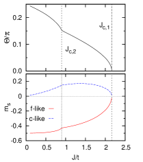
Figure 1: Top: Optimum angle $\Theta$ as a function of $J/t$, $n_{e}=2$, $t_{1}/t=0.3$. Bottom: Ordered moment versus $J/t$.

III Results

Figure 1 shows the angle $\Theta$ which minimizes $E_{0}$ as a function of $J/t$ for $t_{1}/t=0.3$. At approximately $J/t=2.165$ the optimum value of $\Theta$ starts to deviate from zero, indicating a second order transition to the antiferromagnetic phase. It should be noted that no direct Heisenberg exchange between $f$-electrons is included in the Hamiltonian, rather this transition is caused solely by the ‘implicit’ interaction between $f$-spins mediated by the conduction electrons. At $J/t=0.9$ there is an anomaly - i.e. a pronounced upward bend in the curve. This anomaly is absent in the case $t_{1}/t=0$ - see Figure 1 of Ref. afbf . The Figure also shows the $f$-like ordered moment

$$m_{s,f} = \frac{1}{N}\;\sum_{j}\;e^{i{\bm{Q}}\cdot{\bm{R}}_{j}}\langle S_{j,z}\rangle,$$

and an analogous definition for the $c$-like moment. The ordered moments deviate from zero at $J_{c,1}$ and also show the anomaly at $J/t=0.9$. The behavior of the $f$-like ordered moment for $J/t\rightarrow 0$ is somewhat surprising in that its magnitude approaches the saturation value of $1/2$. It should be noted, however, that exactly the same behavior is seen in the Quantum Monte Carlo data for $t_{1}/t=0$ in Ref. Assaad which up to statistical errors are exact results. This highlights the fact that $J/t=0$ is a singular point of the model.

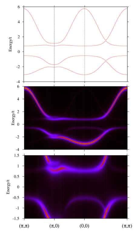
Figure 2: Band structure $E_{\nu,\bf{k}}$ (topmost panel) and spectral density $\rho({\bm{k}},E)$ (lower two panels) for the antiferromagnetic phase of the Kondo insulator, $J/t=1.9$, $t_{1}/t=0.3$. The chemical potential is the zero of energy.

In the following we denote the value of $J$ where the anomaly occurs by $J_{c,2}$. In Ref. afbf it was found that for the case $t_{1}=0$ bond fermion theory predicts the value $J_{c,1}/t=2.3$. As already mentioned this is too large compared to the exact value $J_{c,1}/t=1.45$Assaad , but when $J$ is measured in units of $J_{c,1}$ so that the error in $J_{c,1}/t$ cancels out to some degree, the phase diagram from bond fermion theory is in good agreement with numerical results. Basically the same will be seen to hold true for the band structure.

Figure 3: Quasiparticle gap $\Delta_{QP}$ for $t_{1}/t=0.3$ (top) and $t_{1}/t=0.0$ (bottom) from bond fermion theory (BF) and rescaled bond fermion theory as described in the text (Rescaled) compared to DCA.

To begin with, Figure 2 shows the band structure $E_{\nu,\bf{k}}$ and $c$-like spectral density

$$\rho({\bm{k}},E)=-\frac{1}{\pi}\;Im\;G({\bm{k}},E+i0^{+}),$$

for the antiferromagnetic phase. Here $G({\bm{k}},E)$ is the $c$-electron Green’s function which is readily obtained from the eigenvalues und eigenvectors of $H_{BF}$ and the representation (6). Whereas the band structure shows antiferromagnetic (AF) symmetry this is not at all the case for the spectral density. The individual bands have a strongly ${\bm{k}}$-dependent spectral weight and with the exception of the heavy bands forming the gap around the chemical potential the AF-umklapps have hardly any spectral weight. Along $(0,0)\rightarrow(\pi,\pi)$ in particular this creates the impression as if the strongly dispersive $c$-like band branches into two almost dispersionless bands of low spectral weight. Much the same can be seen in the spectral function obtained by DCA, see Figure 4 in Ref. MartinBerxAssaad and in fact the whole spectral density is quite similar to DCA.
The nature of the anomaly in the $\Theta$ v.s. $J/t$ curve at $J_{c,2}$ seen in Figure 1 becomes clearer in Figure 3. This shows the quasiparticle gap

$$\Delta_{QP}=E_{0}(N_{e}+1)+E_{0}(N_{e}-1)-2E_{0}(N_{e}),$$

as a function of $J/J_{c,1}$. Thereby $E_{0}(N_{e})$ is the ground state energy for $N_{e}$ electrons. In a system described by bands of noninteracting quasiparticles this is the energy gap between the highest occupied and lowest unoccupied energy of the band structure $E_{\nu,\bf{k}}$. For $J/J_{c,1}>1$ there is always a finite gap, that means the system is a paramagnetic insulator. The gap is quite large and to good approximation linear in $J$ - with no indication of the exponential dependence of $T_{K}$ on $J$. At $J_{c,1}$, $\Delta_{QP}$ has an upward kink and then decreases roughly linearly with $J/J_{c,1}$. For $t_{1}/t=0.3$, $\Delta_{QP}$ approaches zero at $J_{c,2}$, whereas for $t_{1}=0$ it extrapolates to zero only at $J=0$. This highlights the importance of Fermi surface nesting for the decoupled conduction electron band. Nonvanishing $t_{1}$ gives a finite dispersion along the antiferromagnetic zone boundary and hence an anisotropic gap. Figure 3 also shows the values of $\Delta_{QP}$ obtained by Martin et al. MartinBerxAssaad by DCA. These authors found $J_{c,1}/t=1.85$, considerably smaller than the value $J_{c,1}/t=2.165$ from bond fermion theory. When both $J$ and $\Delta_{QP}$ are measured in units of $J_{c,1}$, however, the DCA results agree qualitatively with the bond fermion curve, in particular the ratio $J_{c,2}/J_{c,1}\approx 0.4$ for $t_{1}/t=0.3$ is very similar. When the bond fermion values for $\Delta_{QP}/J_{c,1}$ are in addition rescaled by a phenomenological factor of $0.65$ for $t_{1}/t=0.3$ and $0.8$ for $t_{1}/t=0$ the agreement becomes almost perfect for $J>J_{c,2}$ where $\Delta_{QP}$ is so large that it can be resolved in the DCA calculation (the somewhat zigzag shape of the bond Fermion curve is due to the fact that the momenta where the maximum of the lower band/minimum of the upper band are located change with $J/t$). The question then arises as to what is the nature of the ground state for $J\leq J_{c,2}$. Martin et al. arguedMartinBerxAssaad that the system still has a nonvanishing gap even in this parameter range, whereby this gap traces the single impurity Kondo temperature $T_{K}$ which rapidly decreases for small $J/t$ and thus can no longer be resolved by a numerical technique such as DCA for small enough $J/t$. The bond fermion calculation suggests a different interpretation:

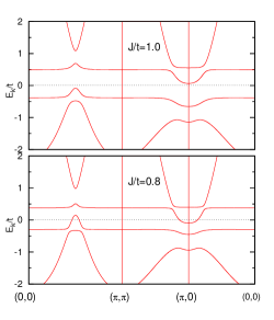
Figure 4: Band structure around $E_{F}$ for $J/t=1.0$ (top) and $J/t=0.8$ (bottom), $t_{1}/t=0.3$.

Figure 4 shows the band structure for two values of $J/t$, one above and one below $J_{c,2}$. The Figure shows that the anomaly corresponds to a transition from an insulator to a semimetal with an electron pocket around $(\pi,0)$ and a hole pocket around $(\frac{\pi}{2},\frac{\pi}{2})$. For $J/t\leq 0.9$ the bond fermion calculation therefore predicts the system to be semimetallic so that $\Delta_{QP}=0$. On the other hand, the transition to the semimetal might also simply indicate the breakdown of the bond fermion description due to its inability to reproduce the energy scale of $T_{K}$. This cannot be decided with the information at hand. Figure 5 shows $J_{c,1}$ and $J_{c,2}$ as functions of $t_{1}/t$.

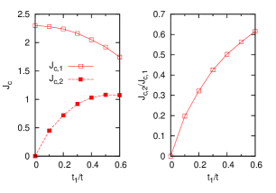
Figure 5: $J_{c,1}$ and $J_{c,2}$ (left) and the ratio $J_{c,2}/J_{c,1}$ (right) versus $t_{1}/t$.

Figure 6: Band structure around $E_{F}$ along $(0,0)\rightarrow(\pi,\pi)$ for different values of $J/t$, $t_{1}/t=0.3$

We now consider in more detail the evolution of the band structure with $J/t$ in the range $J>J_{c,2}$. Figure 6 shows the band structure along $(0,0)\rightarrow(\pi,\pi)$ for different $J/t$ ($t_{1}/t=0.3$). For the relatively large value of $J/t=1.8$ the maximum of the upper occupied band - labeled 2 in Figure 6 - is at $(\pi,\pi)$, the minimum at $(\frac{\pi}{2},\frac{\pi}{2})$. As $J/t$ decreases, the minimum at $(\frac{\pi}{2},\frac{\pi}{2})$ becomes shallower and at $J/t=1.4$ the band is almost dispersionless. Decreasing $J/t$ even more ‘inverts’ the dispersion of the band in that the maximum of the band in question is at $(\frac{\pi}{2},\frac{\pi}{2})$ whereas the minimum is at $(\pi,\pi)$. Exactly the same has also been observed by Martin et al. in their DCA calculation, see Figure 7 in Ref. MartinBerxAssaad . DCA predicts the value of $J/t$ where $(\frac{\pi}{2},\frac{\pi}{2})$ changes from being minimum to being maximum to be around $J/t=1.25=0.68\;J_{c,1}/t$, the bond fermion calculation finds $J/t=1.4=0.65\;J_{c,1}/t$.

Figure 7: Band structure around $E_{F}$ along $(0,0)\rightarrow(\pi,0)$ for different values of $J/t$, $t_{1}/t=0.3$.

Another detail of the evolution of the band structure is shown in Figure 7 which shows the band structure along $(0,0)\rightarrow(\pi,0)$ for larger $J/t$. At $J/t=1.6$ the minimum of the lower unoccupied band - labeled 3 in Figure 7 - is at $(\pi,0)$ (it is this minimum which crosses below $E_{F}$ at $J_{c,2}$). With increasing $J/t$ the difference between the energies at $(0,0)$ and $(\pi,0)$ becomes smaller and for $J/t=1.9$ the band has the same energy at these two momenta. For $J/t=2.0$ the minimum of the band shifts to $(0,0)$. Again, the same behaviour is seen in the DCA spectra, see Figure 8 of Ref. MartinBerxAssaad . DCA finds that the minimum shifts at $J/t=1.55=0.84\;J_{c,1}/t$ whereas the bond fermion calculation gives $J/t=1.90=0.88\;J_{c,1}/t$. As was the case for the phase diagram, bond fermion theory appears to give a ‘rescaled version of reality’: while it does not reproduce absolute energy scales such as the correct $J_{c,1}/t$ or the quasiparticle gap accurately, it reproduces the the band structure and its changes with $J/J_{c,1}$ quite well.

IV Summary and Discussion

In summary we have shown that the bond fermion theory qualitatively reproduces a number of results obtained by numerical methods, in particular the Dynamical Cluster Approximation (DCA) for the KLM. The main deficiency is the overestimation of the value of $J_{c,1}/t$, where the transition to the antiferromagnetic phase occurs. As already mentioned, however, even for numerical methods it is difficult to reproduce this value accurately. The single particle spectral density in the antiferromagnetic phase is in good agreement with DCA and when values of $J$ are measured in units of $J_{c,1}$ the variation of the quasiparticle gap with $J/J_{c,1}$ is similar as obtained by DCA, in particular the value $J_{c,2}/J_{c,1}$ where the quasiparticle gap (approximately) closes is reproduced well. Even fine details in the change of the band structure with $J/J_{c,1}$, such as the shift of band maxima and minima between different point in the Brillouin zone are reproduced well by theory. Interestingly, the shift of the maximum of the topmost occupied band from $(\pi,\pi)$ to $(\frac{\pi}{2},\frac{\pi}{2})$ already foreshadows the Lifshitz transition between the two antiferromagnetic phases for $n_{e}<2$WatanabeOgata ; Asadzadeh ; Kubo ; PetersKawakami , because this is precisely a transition from a pocket around $(\pi,\pi)$ to a pocket around $(\frac{\pi}{2},\frac{\pi}{2})$.
As already mentioned, bond fermion theory is a strong coupling theory by nature and cannot reproduce the single impurity energy scale $T_{K}$. On the other hand, Quantum Monte Carlo finds antiferromagnetic ordering in the 2D KLM for the quite large value $J/t=1.45$ where the quasiparticle gap varies linearly with $J/t$ and no exponential dependence on $J$ is observedAssaad . It is unclear if ordering for such a large value of $J/t$ is special for the planar model but this makes bond Fermion theory useful to discuss antiferromagnetism.
The fact that bond fermion theory describes the KLM reasonably well if $J/t$ is rescaled to lower values can be understood qualitatively by considering the effects of the infinitely strong repulsion between the fermions. First, the repulsion could lead to a reduction of the the hopping integral, $t_{eff}<t$. Second, since presence of a bond fermion at some site $i$ blocks all hopping processes of other fermions involving this site, the repulsion should lead to a loss of kinetic energy per fermion and thus to an increase of the energy $\tilde{e_{0}}$ ascribed to a bond fermion in (7). Since $\tilde{e_{0}}\propto J$ this might have a similar effect as using an effective $J_{eff}>J$ in the bond fermion calculation. Both effects would render $J/t<J_{eff}/t_{eff}$ so if one assumes that the parameters $J$ and $t$ in the above calculations actually correspond to the renormalized $J_{eff}$ and $t_{eff}$ this would explain why the values of $J/t$ have to be reduced to be consistent with numerics. In fact, using a version of bond fermion theory which incorporates the downward renormalization of $t$, Jurecka and Brening found $J_{c,1}/t=1.505$ for $t_{1}=0$JureckaBrenig , remarkably close to the exact value $J_{c,1}/t=1.45$. The way in which the constraint on the bond fermions must be treated needs additional study.
For nonvanishing next-nearest neighbor hopping $t_{1}$ - that means in the absence of $(\pi,\pi)$-nesting for the half-filled decoupled conduction band - bond fermion theory predicts a phase transition to a semimetallic state for small $J/t$. Assuming that a compression of the material would increase the ratio $J/t$ - which is plausible because pressure would tend to increase all hopping integrals and $J$ is proportional to higher powers of these - a hypothetical compound which realizes the semimetallic phase could be driven to the insulating state by applying pressure. This is in contrast to the behaviour of a band insulators with a small gap which would tend to become semimetallic under pressure.

References

- (1) G. R. Stewart, Rev. Mod. Phys. 56, 755 (1984).
- (2) P. A. Lee, T. M. Rice, J. W. Serene, L. J. Sham, and J. W. Wilkins, Comm. in Condensed Matter Phys. 12, 99 (1986).
- (3) G. R. Stewart,Rev. Mod. Phys. 73, 797 (2001).
- (4) H. v. Löhneysen, A. Rosch, M. Vojta, and P. Wölfle, Rev. Mod. Phys. 79, 1015 (2007).
- (5) Q. Si and F. Steglich, Science 329, 1161 (2010).
- (6) A. Yoshimori and A. Sakurai, Progr. Theor. Phys. Supp. 46, 162 (1970).
- (7) C. Lacroix and M. Cyrot, Phys. Rev. B 20, 1969 (1979).
- (8) C. Lacroix, Journal of Magnetism and Magnetic Materials 100, 90 (1991).
- (9) A. Auerbach and K. Levin, Phys. Rev. Lett. 57, 877 (1986).
- (10) S. Burdin, A. Georges, and D. R. Grempel, Phys. Rev. Lett. 85, 1048 (2000).
- (11) G.-M. Zhang and L. Yu, Phys. Rev. B 62, 76 (2000).
- (12) M. Lavagna and C. Pepin, Phys. Rev. B 62, 6450 (2000).
- (13) T. Senthil, M. Vojta, and S. Sachdev, Phys. Rev. B 69, 035111 (2004).
- (14) M. Vojta, Phys. Rev. B 78, 125109 (2008).
- (15) G.-M. Zhang, Y.-H. Su, and L. Yu, Phys. Rev. B 83, 033102 (2011).
- (16) J. Nilsson, Phys. Rev. B 83, 235103 (2011).
- (17) P. Fazekas and E. Müller-Hartmann, Z. Phys. B 85, 285 (1991).
- (18) C. C. Yu and S. R. White, Phys. Rev. Lett. 71, 3866 (1993).
- (19) S. Moukouri and L. G. Caron, Phys. Rev. B. 52,15723(R) (1995).
- (20) S. Moukouri and L. G. Caron, Phys. Rev. B. 54,12212 (1996).
- (21) T. Mutou, N. Shibata, and K. Ueda, Phys. Rev. Lett. 81, 4939 (1998).
- (22) S. Smerat, U. Schollwock, I. P. McCulloch, and H. Schoeller Phys. Rev. B 79, 235107 (2009).
- (23) F. F. Assaad, Phys. Rev. Lett. 83, 796 (1999).
- (24) Z.-P. Shi, R. R. P. Singh, M. P. Gelfand, and Z. Wang Phys. Rev. B 51, 15630(R) (1995).
- (25) W. Zheng and J. Oitmaa, Phys. Rev. B 67, 214406 (2003).
- (26) H. Watanabe and M. Ogata, Phys. Rev. Lett. 99, 136401 (2007).
- (27) M. Z. Asadzadeh, F. Becca, and M. Fabrizio, Phys. Rev. B 87, 205144 (2013).
- (28) K. Kubo, J. Phys. Soc. Jpn. 84, 094702 (2015).
- (29) L. C. Martin and F. F. Assaad, Phys. Rev. Lett. 101, 066404 (2008).
- (30) L. C. Martin, M. Bercx, and F. F. Assaad, Phys. Rev. B 82, 245105 (2010).
- (31) S. Doniach, Physica B 91, 231 (1977).
- (32) J. Kondo, Progress of Theoretical Physics, 32, 37 (1964); K. G. Wilson, Rev. Mod. Phys. 47, 773 (1975).
- (33) M. A. Ruderman and C. Kittel Phys. Rev. 96, 99 (1954); T. Kasuya, Progress of Theoretical Physics, 16, 45 (1956); K. Yosida, Phys. Rev. 106, 893 (1957).
- (34) Q. Si, S. Rabello, K. Ingersent, and J. Smith, Nature 413, 804 (2001).
- (35) Q. Si, S. Rabello, K. Ingersent, and J. L. Smith, Phys. Rev. B 68, 115103 (2003).
- (36) L. De Leo, M. Civelli, and G. Kotliar, Phys. Rev. Lett. 101, 256404 (2008).
- (37) L. Zhu and Q. Si, Phys. Rev. B 66, 024426 (2002).
- (38) J. X. Zhu, D. R. Grempel, and Q. Si, Phys. Rev. Lett. 91, 156404 (2003).
- (39) P. Sun and G. Kotliar, Phys. Rev. Lett. 91, 037209 (2003).
- (40) S. J. Yamamoto and Q. Si, Phys. Rev. Lett. 99, 016401 (2007).
- (41) M. T. Glossop and K. Ingersent, Phys. Rev. Lett. 99, 227203 (2007).
- (42) J.-X. Zhu, S. Kirchner, R. Bulla, and Q. Si, Phys. Rev. Lett. 99, 227204 (2007).
- (43) Q. Si, J. H. Pixley, E. Nica, S. J. Yamamoto, P. Goswami, R. Yu, and S. Kirchner, J. Phys. Soc. Jpn. 83, 061005 (2014).
- (44) E. Abrahams, J. Schmalian, and P. Wölfle, Phys. Rev. B 90, 045105 (2014).
- (45) R. Eder, O. Stoica, and G. A. Sawatzky, Phys. Rev. B. 55, R6109 (1997); R. Eder, O. Rogojanu, and G. A. Sawatzky, Phys. Rev. B. 58, 7599 (1998).
- (46) C. Jurecka and W. Brenig, Phys. Rev. B 64, 092406 (2001).
- (47) R. Eder, K. Grube, and P. Wróbel, Phys. Rev. B 93, 165111 (2016).
- (48) R. Peters and N. Kawakami, Phys. Rev. B 92, 075103 (2015).
- (49) R. Peters and N. Kawakami, Phys. Rev. B 96, 115158 (2017).
- (50) S. Sachdev and R.N. Bhatt, Phys. Rev. B 41, 9323 (1990).
- (51) S. Gopalan, T. M. Rice, and M. Sigrist, Phys. Rev. B 49, 8901 (1994).
- (52) P. Nozieres, Eur. Phys. J. B 6, 447 (1998).
- (53) See, e.g., A. L. Fetter and J. D. Walecka, Quantum Theory of Many Particle Systems (McGraw-Hill, New York, 1971).
- (54) V. N. Kotov, O. Sushkov, ZhengWeihong, and J. Oitmaa, Phys. Rev. Lett. 80, 5790 (1998).
- (55) P. V. Shevchenko, A. W. Sandvik, and O. P. Sushkov Phys. Rev. B 61, 3475 (2000).