One and Two Bit Message Passing for SC-LDPC Codes with Higher-Order Modulation

Abstract

Low complexity decoding algorithms are necessary to meet data rate requirements in excess of $1\text{\,}\mathrm{T}\mathrm{b}\mathrm{p}\mathrm{s}$. In this paper, we study one and two bit message passing algorithms for belief propagation decoding of low-density parity-check (LDPC) codes and analyze them by density evolution. The variable nodes (VNs) exploit soft information from the channel output. To decrease the data flow, the messages exchanged between check nodes (CNs) and VNs are represented by one or two bits. The newly proposed quaternary message passing (QMP) algorithm is compared asymptotically and in finite length simulations to binary message passing (BMP) and ternary message passing (TMP) for spectrally efficient communication with higher-order modulation and probabilistic amplitude shaping (PAS). To showcase the potential for high throughput forward error correction, spatially coupled LDPC codes and a target spectral efficiency (SE) of $3\text{\,}\mathrm{b}\mathrm{i}\mathrm{t}\mathrm{s}\mathrm{/}\mathrm{Q}\mathrm{A}\mathrm{M}\mathrm{s}\mathrm{y}\mathrm{m}\mathrm{b}\mathrm{o}\mathrm{l}$ are considered. Gains of about $0.7\text{\,}\mathrm{d}\mathrm{B}$ and $0.1\text{\,}\mathrm{d}\mathrm{B}$ are observed compared to BMP and TMP, respectively. The gap to unquantized belief propagation (BP) decoding is reduced to about $0.75\text{\,}\mathrm{d}\mathrm{B}$. For smaller code rates, the gain of QMP compared to TMP is more pronounced and amounts to $0.24\text{\,}\mathrm{d}\mathrm{B}$ in the considered example.

I Introduction

Optical coherent transceivers with data rates of $400\text{\,}\mathrm{G}\mathrm{b}\mathrm{p}\mathrm{s}$ are about to be installed in the field [1] and research already considers $1\text{\,}\mathrm{T}\mathrm{b}\mathrm{p}\mathrm{s}$. These data rates require sophisticated optical components, improved digital signal processing algorithms, and FEC (FEC) solutions that can cope with the high speed. While SD (SD) decoders are superior in terms of the NCG (NCG), HD (HD) decoders are appealing when low power consumption and high throughputs are of paramount importance. HD-FEC for optical communications is usually based on product-like codes with RS (RS) or BCH (BCH) component codes of high rate, which can be efficiently decoded via BDD (BDD) (e.g., based on the syndrome). Spatially coupled HD-FEC constructions, such as staircase codes [2] or braided codes [3] achieve additional gains.

Recently, hybrid approaches based on concatenating an inner SD-FEC and an outer HD-FEC have received attention [4, 5]. These ideas have found their way into standards: the optical internet working forum established the 400G ZR standard, a specification to transmit at $400\text{\,}\mathrm{G}\mathrm{b}\mathrm{p}\mathrm{s}$ over data center interconnect links up to $100\text{\,}\mathrm{k}\mathrm{m}$, and agreed on an FEC solution consisting of an inner Hamming code and an outer staircase code, where the inner code decoder is SD and the outer code decoder is HD, with a total of $14.8\%$ overhead and a NCG of $10.8\text{\,}\mathrm{d}\mathrm{B}$.

To exploit the soft-information from the channel, while still only exchanging binary messages during the iterations of BDD, the authors of [6] weight the HD output of the component decoders and recombine it with the soft-information from the channel, after which another HD is made. Similar approaches were also considered in [7, 8], where soft information from the channel is used to exploit particularly reliable and unreliable bits to improve the miscorrection-detection capability of the BDD decoder.

In [9], the authors present a one-bit BMP (BMP) algorithm for LDPC (LDPC) codes. In particular, the VN (VN) processor combines the soft channel message with scaled binary messages from the CN, followed by a HD step. The idea of passing binary messages dates back to the seminal work of Gallager [10], where he presented algorithms that are now called Gallager A and Gallager B.

The internal decoder data flow $F$, defined as the number of bits that are processed in each BP (BP) iteration, is given by

$$F=\frac{2\cdot k_{\text{c}}\cdot q\cdot\bar{d}_{\mathtt{v}}}{R_{\text{c}}}=2\cdot n_{\text{c}}\cdot q\cdot\bar{d}_{\mathtt{v}}$$ (1)

where $k_{\text{c}}$ is the number of information bits, $q$ is the number of bits used to represent a message, $R_{\text{c}}$ is the FEC code rate and $\bar{d}_{\mathtt{v}}$ is average VN degree. Observe that $n_{\text{c}}=k_{\text{c}}/R_{\text{c}}$ is the number of coded bits. Thus, a BMP decoder ($q=1$) allows to reduce the data flow $F$ by a factor of $q$ compared to a decoder using $q$ bits to represent messages. It hereby alleviates the routing congestion problem from which many high throughput, parallel LDPC decoder architectures suffer [11].

The work in [12] extends the BMP algorithm to ternary messages. The third message is an erasure that denotes complete uncertainty about the respective bit value. The algorithm, dubbed TMP (TMP) decoding, closely resembles algorithm E from [13], except that it exploits soft-information at the VN.

These works study decoding for the BSC (BSC) or the AWGN (AWGN) channel with BPSK (BPSK). For coherent, spectrally efficient optical communication, higher-order modulation formats are required and a dedicated code design should take the modulation into account. This is particularly true for PAS (PAS) [14, 15], a coded modulation technique that uses a non-uniform distribution for the constellation points to operate close to the Shannon limit and allows flexible rate adaptation.

The main contributions of this paper are as follows:

• We introduce a QMP (QMP) decoding algorithm as an extension of BMP and TMP. QMP improves the decoding performance for the considered examples by up to $0.24\text{\,}\mathrm{d}\mathrm{B}$ compared to TMP for the same quantization resolution. The gain is particularly pronounced for low FEC code rates.

• We complement the QMP decoding algorithm by deriving its DE (DE) to compute iterative decoding thresholds and obtain the optimal weighting factors required in the decoding algorithm.

• We adapt BMP, TMP, and QMP for higher-order modulation and PAS targeting high-throughput decoding with spectrally efficient signaling and performance close to the Shannon limit by generalizing the DE formulations to take the different BMD (BMD) bit channels into account. Previous work only considered BPSK modulation. We also derive a simplified surrogate channel approach for the initialization of DE for BMD with higher-order modulation.

• We use BMP, TMP, and QMP for SC-LDPC (SC-LDPC) codes and analyze their decoding performance in the finite length regime. The results show that an asymptotic design of the weights via DE also yields very good performance at finite blocklength.

This paper is organized as follows. In Sec. II, we introduce the system model, explain the principles of PAS and review protograph-based SC-LDPC codes. The one bit (BMP) and two bit (TMP, QMP) message passing decoding approaches are described in Sec. III. We develop DE for the three algorithms and higher-order modulation with PAS in Sec. IV. In Sec. V, we present finite length simulation results and compare them to the asymptotic DE predictions. We conclude in Sec. VI.

II Preliminaries

II-A Notation

We refer to the set of natural numbers as $\mathds{N}$; if zero is included, the set is denoted as $\mathds{N}_{0}$. The set of real numbers is $\mathds{R}$, the set of positive real numbers is $\mathds{R}^{+}$ and the set of non-negative real numbers is $\mathds{R}^{+}_{0}$. Other sets are denoted by calligraphic letters such as $\mathcal{A}$. In general, vectors are written in bold font and are assumed to be row vectors, i.e., $\bm{x}=(x_{1},x_{2},\dotsc,x_{n})$. We denote RV with upper case letters, e.g., $X$, and their realizations with lower case letters, e.g., $x$. A discrete RV $X$ has distribution $P_{X}$ on a discrete set $\mathcal{X}$, e.g., for $x\in\mathcal{X}$, $P_{X}(x)=\Pr\{X=x\}$. A continuous RV $X$ takes real values and has density $p_{X}$, e.g., $\int_{-\infty}^{x}p_{X}(\tau)\operatorname{d\!}{\tau}=\Pr\{X\leq x\}$. The expectation of a RV $X$ is denoted by $\operatorname{E}\left[X\right]$. Furthermore, $\operatorname{H}(X)$, $\operatorname{H}(X|Y)$ and $\operatorname{I}(X;Y)$, denote the entropy of the RV $X$, the conditional entropy of the RV $X$ given the RV $Y$ and the mutual information of $X$ and $Y$, respectively.

II-B System Model

Previous works have shown that a discrete time AWGN channel can be considered as an accurate model for dispersion-uncompensated, long-haul optical links [16], where the noise contribution is dominated by amplified spontaneous emission noise from the erbium doped fiber amplifier. A transmitted modulation symbol $X_{i}$ is subject to Gaussian noise $N_{i}$ with zero mean and variance $\sigma^{2}$, and the received samples are

$$Y_{i}=X_{i}+N_{i},\quad i=1,\dotsc,n.$$ (2)

For ease of notation we drop the subscript $i$ whenever possible and we describe the signaling for one real dimension only, i.e., the channel inputs are from an $M$-ary ASK (ASK) set $\mathcal{X}=\{\pm 1,\pm 3,\ldots,\pm(M-1)\}$, where $M$ is even. The extension to a two-dimensional $M^{2}$- QAM (QAM) constellation is straightforward: it can be obtained by the Cartesian product of two real-valued ASK constellations. A four-dimensional dual polarized QAM (DP-QAM) constellation can be obtained as the Cartesian product of two QAM constellations and equivalently, as the Cartesian product of four ASK constellations. The SNR (SNR) is defined as $\text{SNR}=\operatorname{E}\left[X^{2}\right]/\sigma^{2}$.

To use binary FEC codes with higher order modulation formats, we introduce a binary interface for the transmitted constellation points. We define the binary labeling $\chi\colon\mathcal{X}\to\{0,1\}^{m}$ that assigns an $m$-bit binary label $\bm{b}$ to each constellation point $x$, i.e., $\bm{b}=\chi(x)$. For BMD the decoder uses this binary label to calculate a metric for each bit without taking their stochastic dependence into account.

II-C Signaling and Achievable Rates

The maximum rate at which reliable transmission over an AWGN channel is possible is the Shannon capacity [17]. It is achieved when the channel inputs are Gaussian distributed. A uniform distribution on the constellation symbols in $\mathcal{X}$ entails a loss in power efficiency compared to Gaussian signaling. The use of non-uniform probabilities is called PS (PS). Traditionally, the combination of PS and FEC was considered difficult (e.g., see [18, Sec. 6.2], [19]). Recently, the invention of PAS [14] allowed an easy integration of PS with FEC. PAS concatenates a shaping outer code called a DM (DM) [20] and an FEC inner code. This “reverse concatenation” was originally proposed for constrained coding in [21, 22]. The PAS architecture has three properties that distinguishes it from other PS schemes. First, it integrates shaping with existing FEC, second, it achieves the Shannon limit [23, Sec. 10.3], [24], and third, it allows rate adaptation by changing the probability distribution, while leaving the FEC unchanged.

The DM [20] realizes the non-uniform distribution. It takes $k_{\text{dm}}$ uniformly distributed input bits and maps them to a length-$n$ sequence of symbols with the empirical distribution $P_{A}$. For PAS, the DM output set is $\mathcal{A}$ and the DM rate is

$$R_{\text{dm}}=k_{\text{dm}}/n.$$ (3)

The transmission rate $R_{\text{tx}}$ of PAS is [14]

$$R_{\text{tx}}=R_{\text{dm}}+1-(1-R_{\text{c}})\cdot m\quad\text{[$\mathrm{bpcu}$ (bits/channel use)]}$$ (4)

where $R_{\text{c}}$ is the code rate of the FEC code.

An achievable rate for BMD with SD is given by [15]

$$R_{\text{BMD}}(\text{SNR})=\left[\operatorname{H}(\bm{B})-\sum_{k=1}^{m}\operatorname{H}(B_{k}|Y)\right]^{+}\quad[$\mathrm{bpcu}$]$$ (5)

where $[\cdot]^{+}=\max(0,\cdot)$. We introduce $R_{\text{BMD}}^{-1}(\cdot)$ as the inverse function. Its relation to other SD FEC metrics, e.g., the NGMI (NGMI) [25] is explained in [15].

PAS uses the BMD soft-information

$$l_{k}(y)\triangleq\log\frac{P_{B_{k}|Y}(0|y)}{P_{B_{k}|Y}(1|y)},\quad k=1,\dotsc,m$$ (6)

as decoder input, where $P_{B_{k}|Y}(b|y)$ is the probability that the $k$-th bit level of a constellation symbol is equal to $b$ for a given $y$. We have

$$P_{B_{k}|Y}(b|y)\propto\sum_{x\in\mathcal{X}_{k}^{b}}p_{Y|X}(y|x)P_{X}(x)$$ (7)

and $\mathcal{X}_{k}^{b}\triangleq\{x\in\mathcal{X}:[\chi(x)]_{k}=b\}$. The notation $[\bm{b}]_{k}$ refers to the $k$-th component of the vector $\bm{b}$.

II-D Protograph-Based Low-Density Parity-Check Codes

Binary LDPC codes are binary linear block codes defined by an $m_{\text{c}}\times n_{\text{c}}$ sparse parity-check matrix $\bm{H}$. The code dimension is $k_{\text{c}}\geq n_{\text{c}}-m_{\text{c}}$. The Tanner graph of an LDPC code is a bipartite graph $G=(\mathcal{V}\cup\mathcal{C},\mathcal{E})$ consisting of $n_{\text{c}}$ VN and $m_{\text{c}}$ CN. The set $\mathcal{E}$ of edges contains the element $\mathtt{e}_{ij}$, where $\mathtt{e}_{ij}$ is an edge between VN $\mathtt{v}_{j}\in\mathcal{V}$ and CN $\mathtt{c}_{i}\in\mathcal{C}$. Note that $\mathtt{e}_{ij}$ belongs to the set $\mathcal{E}$ if and only if the parity-check matrix element $h_{ij}$ (entry in the $i$-th row and $j$-th column of $\bm{H}$) is equal to $1$. The sets $\mathcal{N}(\mathtt{v}_{j})$ and $\mathcal{N}(\mathtt{c}_{i})$ denote the neighbors of VN $\mathtt{v}_{j}$ and CN $\mathtt{c}_{i}$, respectively. The degree of a VN $\mathtt{v}_{j}$ is denoted by $d_{\mathtt{v}_{j}}$ and it is the cardinality of the set $\mathcal{N}(\mathtt{v}_{j})$. Similarly, the degree of a CN $\mathtt{c}_{i}$ is denoted by $d_{\mathtt{c}_{i}}$ and it is the cardinality of the set $\mathcal{N}(\mathtt{c}_{i})$.

For practical purposes, it is beneficial to impose structure on an LDPC code ensemble. Examples of structured LDPC code ensembles are MET (MET) [26] and protograph-based ensembles [27, 28]. Protograph-based ensembles are defined via a (typically small) basematrix $\bm{B}$ of dimension $m_{\text{p}}\times n_{\text{p}}$ and elements in $\mathds{N}_{0}$. A basematrix may also be represented as a bipartite graph, called a protograph. However, since the elements of the basematrix are not strictly binary, parallel edges are allowed and their numbers correspond to the respective entries in the basematrix. The Tanner graph of an LDPC code can be obtained by lifting a protograph: through copy-and-permute operations copies of the protograph are generated and their edges are permuted such that connectivity constraints imposed by the basematrix are maintained [27]. A protograph-based LDPC code ensemble $\mathcal{C}_{n_{\text{c}}}^{\bm{B}}$ is defined by the set of all length-$n_{\text{c}}$ LDPC codes whose Tanner graph is obtained by lifting $\bm{B}$ by a factor of $Q$ such that $n_{\text{c}}=Q\cdot n_{\text{p}}$. To distinguish the VN and CN in the protograph from those in the lifted parity-check matrix, we introduce the protograph VN set $\mathcal{V}_{\text{p}}=\{\mathtt{V}_{1},\mathtt{V}_{2},\dotsc,\mathtt{V}_{n_{\text{p}}}\}$ and CN set $\mathcal{C}_{\text{p}}=\{\mathtt{C}_{1},\mathtt{C}_{2},\dotsc,\mathtt{C}_{m_{\text{p}}}\}$. Every protograph VN (CN) identifies a VN (CN) type. We use the wording “a type $\mathtt{V}_{i}$ VN” to identify a VN in the lifted Tanner graph of type $\mathtt{V}_{i}$. We also use the convention that a VN $\mathtt{v}_{j}$ in the Tanner graph is of type $\mathtt{V}_{i}$ if $\lceil j/Q\rceil=i$, i.e., consecutive blocks of $Q$ VN in the final parity-check matrix are associated to a given type. The same applies to CN.

II-E Protograph-Based Spatially Coupled LDPC Codes

Consider an SC-LDPC code with a right-unterminated parity-check matrix [29]

$$\bm{H}=\begin{pmatrix}\bm{H}_{0}(0)&&&\\ \bm{H}_{1}(0)&\bm{H}_{0}(1)&&\\ \vdots&\bm{H}_{1}(1)&\bm{H}_{0}(2)&\\ \bm{H}_{\mu}(0)&\vdots&\bm{H}_{1}(2)&\\ &\bm{H}_{\mu}(1)&\vdots&\ddots\\ &&\bm{H}_{\mu}(2)&\ddots\\ &&&\ddots\end{pmatrix}.$$ (8)

In (8), $\mu$ denotes the syndrome former memory of the SC-LDPC code. The index in brackets denotes the spatial position. If the matrices $\bm{H}_{i}(s),i\in\{0,\dotsc,\mu\}$, are the same for all spatial positions $s\in\{0,\dotsc,S-1\}$, the SC-LDPC code is called time-invariant and the index $s$ can be dropped. The dimension of the matrices $\bm{H}_{i}(s)$ is $m_{\text{c}}^{\text{SC}}\times n_{\text{c}}^{\text{SC}}$.

Because of the diagonal structure of $\bm{H}$, a CN is connected to at most $(\mu+1)n_{\text{c}}^{\text{SC}}$ VN. This allows using a window decoding approach [30] that reduces latency, increases throughput, and makes SC-LDPC codes particularly interesting for optical communications [29].

SC-LDPC codes are known to exhibit a phenomenon known as threshold saturation [31] that allows to approach the bit-wise MAP (MAP) decoding threshold of the underlying block code with (unquantized) BP decoding.

SC-LDPC codes can be constructed from protographs and have the structure

$$\bm{B}=\begin{pmatrix}\bm{B}_{0}&&&\\ \bm{B}_{1}&\bm{B}_{0}&&\\ \vdots&\bm{B}_{1}&\bm{B}_{0}&\\ \bm{B}_{\mu}&\vdots&\bm{B}_{1}&\\ &\bm{B}_{\mu}&\vdots&\ddots\\ &&\bm{B}_{\mu}&\ddots\\ &&&\ddots\end{pmatrix}.$$ (9)

The protograph in (9) is then lifted by a factor of $Q$ to obtain the final parity-check matrix $\bm{H}$.

For practical operation, the SC-LDPC code is commonly terminated after a number of $S$ spatial positions. Due to this termination, a rate loss occurs that vanishes for large $S$. The resulting code rate is

$$R_{\text{c}}=1-\frac{\mu+S}{S}\frac{m_{\text{p}}^{\text{SC}}}{n_{\text{p}}^{\text{SC}}}=1-\left(1+\frac{\mu}{S}\right)\frac{m_{\text{p}}^{\text{SC}}}{n_{\text{p}}^{\text{SC}}}$$ (10)

where the basematrices $\bm{B}_{0},\dotsc,\bm{B}_{\mu}$ have dimensions $m_{\text{p}}^{\text{SC}}\times n_{\text{p}}^{\text{SC}}$. The overall size of the matrix $\bm{B}$ is $m_{\text{p}}\times n_{\text{p}}=(\mu+S)m_{\text{p}}^{\text{SC}}\times n_{\text{p}}^{\text{SC}}S$.

III Decoding Algorithms for One And Two Bit Message Passing

In this section, we first review the BMP and TMP decoding algorithms introduced in [9] and [12, Sec. III-A]. In Sec. III-B, we then present a new decoding algorithm that takes full advantage of $2$-bit messages, which we dub QMP.

For the described algorithms, we denote by $m_{\mathtt{c}\to\mathtt{v}}^{(\ell)}$ the message sent from CN $\mathtt{c}$ to its neighboring VN $\mathtt{v}$ at the $\ell$-th iteration. Similarly, $m_{\mathtt{v}\to\mathtt{c}}^{(\ell)}$ is the message sent from VN $\mathtt{v}$ to CN $\mathtt{c}$. The soft information at the input of the decoder for the $j$-th coded bit is denoted by $l_{\text{dec},j}$ and calculated according to (6).

III-A Binary and Ternary Message Passing

For BMP, the exchanged messages are binary, i.e., $m_{\mathtt{v}\to\mathtt{c}}^{(\ell)},m_{\mathtt{c}\to\mathtt{v}}^{(\ell)}\in\mathcal{M}_{\text{BMP}}\triangleq\{-1,+1\}$. For TMP, the exchanged messages are ternary and we have $m_{\mathtt{v}\to\mathtt{c}}^{(\ell)},m_{\mathtt{c}\to\mathtt{v}}^{(\ell)}\in\mathcal{M}_{\text{TMP}}\triangleq\{-1,0,+1\}$. A message value of zero indicates complete uncertainty about the respective bit.

In every decoding iteration, each VN and CN computes extrinsic messages that are forwarded to the neighboring nodes. Specifically, the message from VN $\mathtt{v}$ to CN $\mathtt{c}$ is obtained by combining the channel soft-information $l_{\text{dec}}$ with a weighted version of all other incoming CN messages. Finally, a quantization function $\Psi\colon\mathds{R}\to\mathcal{M}$ is applied to turn the result into binary and ternary messages for BMP and TMP, respectively. The weighting factors $w_{ij}^{(\ell)}$ are real valued and depend on the current iteration number. They can be obtained from the DE analysis as shown in Sec. IV. The quantization function is

$$\Psi(x)=\begin{cases}+1,&x>0\\ -1,&x\leq 0\end{cases}$$ (11)

for BMP and

$$\Psi(x)=\begin{cases}+1,&x>T\\ 0,&-T\leq x\leq T\\ -1,&x<-T\end{cases}$$ (12)

for TMP. The equality signs in (11) and (12) are chosen such that ties are broken. Note that the threshold parameter $T\in\mathds{R}^{+}_{0}$ in (12) depends on the SNR and needs to be chosen for each signaling mode and iteration individually to minimize the decoding threshold. However, numerical studies reveal that a single value that is kept constant over the iterations entails almost no loss in performance. Therefore, we resort to this setting in the following.

For the CN to VN update, a CN sends the product of incoming messages from the other neighboring VN. In the last iteration $\ell_{\text{max}}$, the a-posteriori estimate of each codeword bit is calculated by taking a hard decision on the combined soft-information from all CN neighbors and the channel. The algorithmic procedure for BMP and TMP decoding is summarized in Algorithm 1. The weighting factors $w_{ij}^{(\ell)}$ have been derived as part of the DE for BMP and TMP in [12].

Set $m_{\mathtt{v}_{j}\to\mathtt{c}_{i}}^{(0)}=\Psi(l_{\text{dec},j}),\forall j=1,\ldots,n_{\text{c}},\forall\mathtt{c}_{i}\in\mathcal{N}(\mathtt{v}_{j})$.

$\ell=0$

while $\ell\leq\ell_{\text{max}}$ do

     // CN update

     for $i=1,\dotsc,m{{}_{\text{c}}}$ do

         for $\mathtt{v}_{j}\in\mathcal{N}(\mathtt{c}_{i})$ do

              $m_{\mathtt{c}_{i}\to\mathtt{v}_{j}}^{(\ell)}=\prod\limits_{\mathtt{v}_{j^{\prime}}\in\mathcal{N}(\mathtt{c}_{i})\setminus\{\mathtt{v}_{j}\}}m_{\mathtt{v}_{j^{\prime}}\to\mathtt{c}_{i}}^{({\ell-1})}$

         end for

     end for

     // VN update

     for $j=1,\dotsc,n{{}_{\text{c}}}$ do

         for $\mathtt{c}_{i}\in\mathcal{N}(\mathtt{v}_{j})$ do

              $m_{\mathtt{v}_{j}\to\mathtt{c}_{i}}^{(\ell)}=\Psi\left(l_{\text{dec},j}+\sum\limits_{\mathtt{c}_{i^{\prime}}\in\mathcal{N}(\mathtt{v}_{j})\setminus\{\mathtt{c}_{i}\}}w_{i^{\prime}j}^{(\ell)}m_{\mathtt{c}_{i^{\prime}}\to\mathtt{v}_{j}}^{(\ell)}\right)$

         end for

     end for

     $\ell=\ell+1$

end while

// Final codeword bit estimate

for $j=1,\dotsc,n{{}_{\text{c}}}$ do

     $\hat{c}_{j}=\frac{1}{2}-\frac{1}{2}\operatorname*{sign}\left(l_{\text{dec},j}+\sum\limits_{\mathtt{c}_{i}\in\mathcal{N}(\mathtt{v}_{j})}w_{ij}^{(\ell_{\text{max}})}m_{\mathtt{c}_{i}\to\mathtt{v}_{j}}^{(\ell_{\text{max}})}\right)$

end for

Algorithm 1 BMP and TMP decoding.

III-B Quaternary Message Passing

The TMP algorithm of Sec. III-A requires two bits per exchanged message. We now introduce a QMP decoding algorithm that requires the same number of bits per exchanged message, but allows a more granular quantization of the associated reliability soft-information.

The key idea of QMP is to distinguish between low and high reliability messages. The VN to CN and CN to VN messages, $m_{\mathtt{v}\to\mathtt{c}}^{(\ell)}$ and $m_{\mathtt{c}\to\mathtt{v}}^{(\ell)}$, take values in the quaternary alphabet $\mathcal{M}_{\text{QMP}}\triangleq\{-\mathtt{H},-\mathtt{L},+\mathtt{L},+\mathtt{H}\}$ and $\mathtt{L}$ and $\mathtt{H}$ correspond to messages with low and high reliability, respectively. The quantization function is

$$\Psi(x)=\begin{cases}-\mathtt{H},&x\leq-T\\ -\mathtt{L},&-T<x<0\\ +\mathtt{L},&0\leq x<T\\ +\mathtt{H},&x\geq T.\end{cases}$$ (13)

The QMP decoding algorithm is summarized in Algorithm 2. At the CN, a min-sum decoding rule is employed. At the VN, the incoming messages are weighted and combined with the channel soft-information. In contrast to BMP and TMP, two sets of weighting factors are needed for QMP depending on the magnitude of the received message. The weights $w_{ij,\mathtt{L}}^{(\ell)}$ are used for messages with low reliability (i.e., $m_{\mathtt{c}\to\mathtt{v}}\in\{-\mathtt{L},+\mathtt{L}\})$, whereas $w_{ij,\mathtt{H}}^{(\ell)}$ are used for messages with high reliability (i.e., $m_{\mathtt{c}\to\mathtt{v}}\in\{-\mathtt{H},+\mathtt{H}\}$).

Set $m_{\mathtt{v}_{j}\to\mathtt{c}_{i}}^{(0)}=\Psi(l_{\text{dec},j}),\forall j=1,\ldots,n_{\text{c}},\forall\mathtt{c}_{i}\in\mathcal{N}(\mathtt{v}_{j})$.

$\ell=0$

while $\ell\leq\ell_{\text{max}}$ do

     // CN update

     for $i=1,\dotsc,m{{}_{\text{c}}}$ do

         for $\mathtt{v}_{j}\in\mathcal{N}(\mathtt{c}_{i})$ do

              $\begin{aligned} m_{\mathtt{c}_{i}\to\mathtt{v}_{j}}^{(\ell)}=&\min\limits_{\mathtt{v}_{j^{\prime}}\in\mathcal{N}(\mathtt{c}_{i})\setminus\{\mathtt{v}_{j}\}}|m_{\mathtt{v}_{j^{\prime}}\to\mathtt{c}_{i}}^{(\ell-1)}|\cdot\\ &\prod\limits_{\mathtt{v}_{j^{\prime}}\in\mathcal{N}(\mathtt{c}_{i})\setminus\{\mathtt{v}_{j}\}}\operatorname*{sign}\left(m_{\mathtt{v}_{j^{\prime}}\to\mathtt{c}_{i}}^{(\ell-1)}\right)\end{aligned}$

         end for

     end for

     // VN update

     for $j=1,\dotsc,n{{}_{\text{c}}}$ do

         for $\mathtt{c}_{i}\in\mathcal{N}(\mathtt{v}_{j})$ do

              $l_{\text{av}}^{(\ell)}=\sum\limits_{\mathtt{c}_{i^{\prime}}\in\mathcal{N}\left(\mathtt{v}_{j}\right)\setminus\{\mathtt{c}_{i}\}}\operatorname*{sign}(m^{(\ell)}_{\mathtt{c}_{i^{\prime}}\to\mathtt{v}_{j}})w^{(\ell)}_{i^{\prime}j,|m^{(\ell)}_{\mathtt{c}_{i^{\prime}}\to\mathtt{v}_{j}}|}$

              $m_{\mathtt{v}_{j}\to\mathtt{c}_{i}}^{(\ell)}=\Psi\left(l_{\text{dec},j}+l_{\text{av}}^{(\ell)}\right)$

         end for

     end for

     $\ell=\ell+1$

end while

// Final codeword bit estimate

for $j=1,\dotsc,n{{}_{\text{c}}}$ do

     $l_{\text{in}}=\sum\limits_{\mathtt{c}_{i}\in\mathcal{N}\left(\mathtt{v}_{j}\right)}\operatorname*{sign}(m^{(\ell_{\text{max}})}_{\mathtt{c}_{i}\to\mathtt{v}_{j}})w^{(\ell_{\text{max}})}_{ij,|m^{(\ell)}_{\mathtt{c}_{i}\to\mathtt{v}_{j}}|}$

     $\hat{c}_{j}=\frac{1}{2}-\frac{1}{2}\operatorname*{sign}\left(l_{\text{dec},j}+l_{\text{in}}\right)$

end for

Algorithm 2 QMP decoding.

IV Density Evolution Analysis for QMP

In the following, we describe DE for QMP and protograph-based LDPC code ensembles. The purpose of DE is twofold. First, it provides asymptotic decoding thresholds of the considered ensembles. Second, it allows to compute the optimal weighting factors for the VN update that are needed for the decoding algorithm (optimal in an asymptotic sense, i.e., for infinite block length and lifting factor).

IV-A Symmetry

DE analysis for binary LDPC codes [13] assumes that the channel message and the extrinsic decoder messages fulfill the symmetry constraint

$$p_{L|B}(l|0)=p_{L|B}(-l|1)$$ (14)

where the RV $L$ denotes the soft-information calculated from the channel output. In this case, one can assume that the all-zero codeword is transmitted and track the probability of decoding failure over the iterations. As pointed out in [32], for BMD with higher-order modulation, the bit channels $p_{L_{k}|B_{k}}$ are generally not symmetric, where the RV $L_{k}$ is defined as (cf. (6))

$$L_{k}\triangleq\log\frac{P_{B_{k}|Y}(0|Y)}{P_{B_{k}|Y}(1|Y)},\quad k=1,\dotsc,m.$$ (15)

However, we can use channel adapters [32] to introduce symmetrized counterparts. This can be accomplished by using a pseudo-random, binary scrambling sequence at both the transmitter and receiver, which modifies (15) as

$$\tilde{L}_{k}=L_{k}\cdot(1-2B_{k}).$$ (16)

The resulting bit-channels $p_{\tilde{L}_{k}|B_{k}}$ are symmetric, i.e., we have

$$p_{\tilde{L}_{k}|B_{k}}(l|0)=p_{\tilde{L}_{k}|B_{k}}(-l|1).$$ (17)

IV-B Initialization of Density Evolution for Different Bit Channels

We associate with each VN type a bit level. Let $\phi(j)$ be the bit level on which the VN of type $\mathtt{V}_{j}$ are mapped and let $\mathcal{V}_{\text{p}}^{(k)}\subseteq\mathcal{V}_{\text{p}}$ be the subset of protograph VN that are mapped to the $k$-th bit level. We assume that the number $n_{\text{p}}$ of VN in the protograph is an integer multiple of $m$, such that each bit level is assigned to $n_{\text{p}}/m$ VN.

Let $p_{\mathtt{m}}^{(\ell)}(i,j)$ be the probability that the message sent from $\mathtt{V}_{j}$ to $\mathtt{C}_{i}$ at the $\ell$-th iteration on one of the $b_{ij}$ edges connecting $\mathtt{V}_{j}$ to $\mathtt{C}_{i}$ is equal to $\mathtt{m}\in\{-\mathtt{H},-\mathtt{L},+\mathtt{L}\}$. To initialize DE, we calculate the initial message probabilities as

$$p_{-\mathtt{H}}^{(0)}(i,j) =\int_{-\infty}^{-T}p_{\tilde{L}_{\phi(j)}|B_{\phi(j)}}(l|0)\operatorname{d\!}{l}$$ (18)

$$p_{-\mathtt{L}}^{(0)}(i,j) =\int_{-T}^{0}p_{\tilde{L}_{\phi(j)}|B_{\phi(j)}}(l|0)\operatorname{d\!}{l}$$ (19)

$$p_{+\mathtt{L}}^{(0)}(i,j) =\int_{0}^{T}p_{\tilde{L}_{\phi(j)}|B_{\phi(j)}}(l|0)\operatorname{d\!}{l}.$$ (20)

The integrals in (18)–(20) do not allow a closed form solution, but can be calculated by means of Monte Carlo simulations or transformations of RV. Note that the above calculations need to be performed only once.

In Fig. 1, we show the CDF $\Pr\{\tilde{L}_{k}\leq l\}$ for 8-ASK with uniform and PS signaling obtained via Monte Carlo simulations. The CDF can be used to calculate (18)–(20) as

$$p_{-\mathtt{H}}^{(0)}(i,j) =\Pr\{\tilde{L}_{\Phi(j)}\leq-T\},$$ (21)

$$p_{-\mathtt{L}}^{(0)}(i,j) =\Pr\{\tilde{L}_{\Phi(j)}\leq 0\}-\Pr\{\tilde{L}_{\Phi(j)}\leq-T\},$$ (22)

$$p_{+\mathtt{L}}^{(0)}(i,j) =\Pr\{\tilde{L}_{\Phi(j)}\leq T\}-\Pr\{\tilde{L}_{\Phi(j)}\leq 0\}.$$ (23)

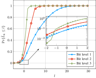
(a)

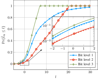
(b)

Figure 1: Comparison of CDF plots for 8-ASK with uniform and PS signaling. Both scenarios are for $\text{SNR}=$9\text{\,}\mathrm{d}\mathrm{B}$$. PS signaling uses an MB distribution with entropy $\operatorname{H}(X)=$2.25\text{\,}\mathrm{b}\mathrm{i}\mathrm{t}\mathrm{s}$$. The dashed lines in the insets denote the CDFs obtained via the surrogate approach.

IV-C Density Evolution for QMP

Similarly to before, let $q_{\mathtt{m}}^{(\ell)}(i,j)$ denote the probability that the message sent from $\mathtt{C}_{i}$ to $\mathtt{V}_{j}$ at the $\ell$-th iteration is equal to $\mathtt{m}\in\mathcal{M}_{\text{QMP}}$.

1. Initialization. For $j=1,2,\ldots,n_{\text{p}}$ and $i=1,2,\ldots,m_{\text{p}}$ with $b_{ij}\neq 0$, compute $p^{(0)}_{-\mathtt{H}}(i,j)$, $p^{(0)}_{-\mathtt{L}}(i,j)$ and $p^{(0)}_{+\mathtt{L}}(i,j)$ according to (18), (19) and (20).

2. For $\ell=1,2,\ldots,\ell_{\text{max}}$ repeat the following three update steps

   Check to variable update. For $j=1,2,\ldots,n_{\text{p}}$ and $i=1,2,\ldots,m_{\text{p}}$, if $b_{ij}\neq 0$ then compute

   $$q^{(\ell)}_{-\mathtt{H}}(i,j)=\frac{1}{2}\left[\prod\limits_{b_{is}\neq 0}\left(1-p^{(\ell-1)}_{-\mathtt{L}}(i,s)-p^{(\ell-1)}_{+\mathtt{L}}(i,s)\right)^{b_{is}-\delta_{sj}}\right.$$ (24)

   $$\left.-\prod\limits_{b_{is}\neq 0}\left(1-2p^{(\ell-1)}_{-\mathtt{H}}(i,s)-p^{(\ell-1)}_{-\mathtt{L}}(i,s)-p^{(\ell-1)}_{+\mathtt{L}}(i,s)\right)^{b_{is}-\delta_{sj}}\right]$$

   $$q^{(\ell)}_{-\mathtt{L}}(i,j)=\frac{1}{2}\left[1-\prod\limits_{b_{is}\neq 0}\left(1-p^{(\ell-1)}_{-\mathtt{L}}(i,s)-p^{(\ell-1)}_{+\mathtt{L}}(i,s)\right)^{b_{is}-\delta_{sj}}\right.$$ (25)

   $$-\prod\limits_{b_{is}\neq 0}\left(1-2p^{(\ell-1)}_{-\mathtt{H}}(i,s)-2p^{(\ell-1)}_{-\mathtt{L}}(i,s)\right)^{b_{is}-\delta_{sj}}$$

   $$\left.+\prod\limits_{b_{is}\neq 0}\left(1-2p^{(\ell-1)}_{-\mathtt{H}}(i,s)-p^{(\ell-1)}_{-\mathtt{L}}(i,s)-p^{(\ell-1)}_{+\mathtt{L}}(i,s)\right)^{b_{is}-\delta_{sj}}\right]$$

   $$q^{(\ell)}_{+\mathtt{L}}(i,j)=\frac{1}{2}\left[1-\prod\limits_{b_{is}\neq 0}\left(1-p^{(\ell-1)}_{-\mathtt{L}}(i,s)-p^{(\ell-1)}_{+\mathtt{L}}(i,s)\right)^{b_{is}-\delta_{sj}}\right.$$ (26)

   $$+\prod\limits_{b_{is}\neq 0}\left(1-2p^{(\ell-1)}_{-\mathtt{H}}(i,s)-2p^{(\ell-1)}_{-\mathtt{L}}(i,s)\right)^{b_{is}-\delta_{sj}}$$

   $$\left.-\prod\limits_{b_{is}\neq 0}\left(1-2p^{(\ell-1)}_{-\mathtt{H}}(i,s)-p^{(\ell-1)}_{-\mathtt{L}}(i,s)-p^{(\ell-1)}_{+\mathtt{L}}(i,s)\right)^{b_{is}-\delta_{sj}}\right].$$

   Variable to check update. For $j=1,2,\ldots,n_{\text{p}}$ and $i=1,2,\ldots,m_{\text{p}}$, if $b_{ij}\neq 0$, compute

   $$\begin{split}p^{(\ell)}_{-\mathtt{H}}(i,j)=&\sum\limits_{z}\Pr\left\{L^{(\ell)}_{\text{av}}=z\right\}\Pr\{\tilde{L}_{\phi(j)}\leq-T-z\}\end{split}$$ (27)

   $$\begin{split}p^{(\ell)}_{-\mathtt{L}}(i,j)=&\sum\limits_{z}\Pr\left\{L^{(\ell)}_{\text{av}}=z\right\}\Pr\{-T-z<\tilde{L}_{\phi(j)}<-z\}\end{split}$$ (28)

   $$\begin{split}p^{(\ell)}_{+\mathtt{L}}(i,j)=&\sum\limits_{z}\Pr\left\{L^{(\ell)}_{\text{av}}=z\right\}\Pr\{-z\leq\tilde{L}_{\phi(j)}<T-z\}\end{split}$$ (29)

   where $L^{(\ell)}_{\text{av}}$ is a RV representing the sum of the LLR of the $d_{\mathtt{v}_{j}}-1$ CN messages at the input of $\mathtt{V}_{j}$ at the $\ell$-th iteration. We have

   $$\Pr\left\{L^{(\ell)}_{\text{av}}=z\right\}=\sum\limits_{\bm{u},\bm{v},\bm{t}}\prod\limits_{b_{sj}\neq 0}{\textstyle\binom{b_{sj}-\delta_{si}}{u_{s},v_{s},t_{s},b_{sj}-\delta_{si}-u_{s}-v_{s}-t_{s}}}\cdot$$ (30)

   $$q^{(\ell)}_{-\mathtt{H}}(s,j)^{u_{s}}q^{(\ell)}_{-\mathtt{L}}(s,j)^{v_{s}}q^{(\ell)}_{+\mathtt{L}}(s,j)^{t_{s}}\cdot$$

   $$\left(1-q^{(\ell)}_{-\mathtt{H}}(s,j)-q^{(\ell)}_{-\mathtt{L}}(s,j)-q^{(\ell)}_{+\mathtt{L}}(s,j)\right)^{b_{sj}-\delta_{si}-u_{s}-v_{s}-t_{s}}$$

   where the outer sum is over all integer vector triplets $\bm{u},\bm{v}$ and $\bm{w}$ for which

   $$\sum\limits_{e=1}^{m_{\text{p}}} \left[w_{ej,\mathtt{L}}^{(\ell)}(t_{e}-v_{e})+\right.$$ (31)

   $$\left.w_{ej,\mathtt{H}}^{(\ell)}(b_{ej}-\delta_{ei}-2u_{e}-v_{e}-t_{e})\right]=z$$

   with

   $$w_{ej,\mathtt{L}}^{(\ell)}=\ln\left(\dfrac{q^{(\ell)}_{+\mathtt{L}}(e,j)}{q^{(\ell)}_{-\mathtt{L}}(e,j)}\right)$$ (32)

   and

   $$w_{ej,\mathtt{H}}^{(\ell)}=\ln\left(\dfrac{1-q^{(\ell)}_{-\mathtt{H}}(e,j)-q^{(\ell)}_{-\mathtt{L}}(e,j)-q^{(\ell)}_{+\mathtt{L}}(e,j)}{q^{(\ell)}_{-\mathtt{H}}(e,j)}\right).$$ (33)

   Specifically, the entries $u_{s}$, $v_{s}$, and $t_{s}$ represent the number of messages $-\mathtt{H}$, $-\mathtt{L}$ and $+\mathtt{L}$, respectively, that $\mathtt{C}_{s}$ sends to $\mathtt{V}_{j}$ on $b_{sj}-\delta_{si}$ of the $b_{sj}$ edges connecting $\mathtt{C}_{s}$ to $\mathtt{V}_{j}$. Thus, for $s=1,2,\ldots,m_{\text{p}}$ we have $0\leq u_{s},v_{s},t_{s}$ and $u_{s}+v_{s}+t_{s}\leq b_{sj}-\delta_{si}$.

   A-posteriori update. For $j=1,2,\ldots,n_{\text{p}}$, compute

   $$P_{\text{app}}^{(\ell)}(j)=\sum\limits_{z}\Pr\left\{L^{(\ell)}_{\text{in}}=z\right\}\Pr\left\{\tilde{L}_{\phi(j)}\leq-z\right\}$$ (34)

   where ${L}^{(\ell)}_{\text{in}}$ is a RV representing the sum of the LLR of all incoming $d_{\mathtt{v}_{j}}$ CN messages at the input of $\mathtt{V}_{j}$ at the $\ell$-th iteration. We have

   $$\Pr\left\{L^{(\ell)}_{\text{in}}=z\right\}=\sum\limits_{{\bm{u}},{\bm{v}},{\bm{t}}}\prod\limits_{b_{sj}\neq 0}{\textstyle\binom{b_{sj}}{{u}_{s},{v}_{s},{t}_{s},b_{sj}-{u}_{s}-{v}_{s}-{t}_{s}}}\cdot$$ (35)

   $$q^{(\ell)}_{-\mathtt{H}}(s,j)^{{u}_{s}}q^{(\ell)}_{-\mathtt{L}}(s,j)^{{v}_{s}}q^{(\ell)}_{+\mathtt{L}}(s,j)^{{t}_{s}}\cdot$$

   $$\left(1-q^{(\ell)}_{-\mathtt{H}}(s,j)-q^{(\ell)}_{-\mathtt{L}}(s,j)-q^{(\ell)}_{+\mathtt{L}}(s,j)\right)^{b_{sj}-{u}_{s}-{v}_{s}-{t}_{s}}$$

   where the outer sum is over all integer vector triplets ${\bm{u}},{\bm{v}}$ and ${\bm{t}}$ for which

   $$\sum\limits_{e=1}^{m_{\text{p}}} \left[w_{ej,\mathtt{L}}^{(\ell)}({t}_{e}-{v}_{e})+w_{ej,\mathtt{H}}^{(\ell)}(b_{ej}-2{u}_{e}-{v}_{e}-{t}_{e})\right]=z$$ (36)

   where $w_{ej,\mathtt{L}}^{(\ell)}$ and $w_{ej,\mathtt{H}}^{(\ell)}$ are given in (32) and (33). The vector elements ${u}_{s}$, ${v}_{s}$, and ${t}_{s}$ represent the number of messages $-\mathtt{H}$, $-\mathtt{L}$ and $+\mathtt{L}$, respectively, that $\mathtt{C}_{s}$ sends to $\mathtt{V}_{j}$ on the $b_{sj}$ edges connecting $\mathtt{C}_{s}$ to $\mathtt{V}_{j}$. Thus, for $s=1,2,\ldots,m_{\text{p}}$ we have $0\leq{u}_{s},{v}_{s},{t}_{s}$ and ${u}_{s}+{v}_{s}+{t}_{s}\leq b_{sj}$.

Remark 1.

With a slight abuse of notation, the weighting factors for QMP in Algorithm 2 are calculated from those derived in this section as

$$w_{ij,\mathtt{H}}^{(\ell)}\Leftrightarrow w_{\lceil i/Q\rceil\lceil j/Q\rceil,\mathtt{H}}^{(\ell)}$$ (37)

$$w_{ij,\mathtt{L}}^{(\ell)}\Leftrightarrow w_{\lceil i/Q\rceil\lceil j/Q\rceil,\mathtt{L}}^{(\ell)}$$ (38)

for $i=1,\dotsc,m_{\text{c}}$ and $j=1,\dotsc,n_{\text{c}}$.

Remark 2.

Practical decoder implementations may also quantize the weighting factors or share the same weighting factors for several iterations. Similar decoding approaches for product codes [6] suggest only minimal performance degradation in this case [33].

IV-D Surrogate Channel Approach for the Density Evolution Initialization

As an alternative to Monte Carlo simulations, we may resort to a surrogate channel approach [34, 35, 36] to approximate the required input probabilities (18)–(20). For this, the bit-channels $p_{\tilde{L}_{k}|B_{k}}$ are replaced by “equivalent” AWGN channels with uniform binary inputs for which the derivation of the CDF is easier. We establish their “equivalence” by requiring that the channel and its surrogate have the same channel uncertainty. Let the surrogate be $\breve{Y}_{k}=\breve{X}_{k}+\breve{N}_{k}$ with $\breve{X}_{k}\in\{-1,+1\}$ and $\breve{N}_{k}\sim\mathcal{N}(0,\breve{\sigma}_{k}^{2})$ for $k=1,\ldots,m$. For each SNR, we calculate the set of equivalent channel parameters

$$\breve{\sigma}_{k}^{2}:\operatorname{H}(\breve{B}_{k}|\breve{Y})=\operatorname{H}(B_{k}|Y),\quad k=1,\ldots,m.$$ (39)

For QMP we obtain the expressions

$$\begin{split}p^{(0)}_{-\mathtt{H}}(i,j)=Q\left(\dfrac{T+\mu_{\text{ch},\phi(j)}}{\sigma_{\text{ch},\phi(j)}}\right)\end{split}$$ (40)

$$\begin{split}p^{(0)}_{-\mathtt{L}}(i,j)=Q\left(\dfrac{\mu_{\text{ch},\phi(j)}}{\sigma_{\text{ch},\phi(j)}}\right)-Q\left(\dfrac{T+\mu_{\text{ch},\phi(j)}}{\sigma_{\text{ch},\phi(j)}}\right)\end{split}$$ (41)

$$\begin{split}p^{(0)}_{+\mathtt{L}}(i,j)=Q\left(\dfrac{-T+\mu_{\text{ch},\phi(j)}}{\sigma_{\text{ch},\phi(j)}}\right)-Q\left(\dfrac{\mu_{\text{ch},\phi(j)}}{\sigma_{\text{ch},\phi(j)}}\right)\end{split}$$ (42)

where $\mu_{\text{ch},k}=2/{\breve{\sigma}_{k}^{2}}$, $\sigma_{\text{ch},k}^{2}=4/{\breve{\sigma}_{k}^{2}}$, and $Q(\cdot)$ is the standard normal Gaussian tail probability, i.e.,

$$Q(x)=\int_{x}^{\infty}(1/\sqrt{2\pi})\exp(-\tau^{2}/2)\operatorname{d\!}{\tau}.$$ (43)

In Fig. 1, we show the approximations of the true CDF by the surrogate approach (dashed lines). A close match of the true CDF and their approximations is observed.

IV-E Density Evolution of Window Decoding for Spatially Coupled Low-Density Parity-Check Codes

We follow the approach of [37] to determine the decoding threshold of protograph-based SC-LDPC code ensembles for window decoding. For this, we apply the DE analysis of Sec. IV for the respective decoding algorithm on a protograph matrix $\bm{B}_{[1:W,1:W]}$ that has been derived from (9) for a given decoding window size of $W$ with $\mu+1\leq W\leq L$. The notation $\bm{B}_{[1:W,1:W]}$ denotes the block matrix of size $W\times W$ that is formed from the first $W$ block rows and $W$ block columns of $\bm{B}$. For instance, for $\mu=2$ and $W=4$ we have

$$\bm{B}_{[1:4,1:4]}=\begin{pmatrix}\bm{B}_{0}&\bm{0}&\bm{0}&\bm{0}\\ \bm{B}_{1}&\bm{B}_{0}&\bm{0}&\bm{0}\\ \bm{B}_{2}&\bm{B}_{1}&\bm{B}_{0}&\bm{0}\\ \bm{0}&\bm{B}_{2}&\bm{B}_{1}&\bm{B}_{0}\end{pmatrix}.$$ (44)

Convergence of the window decoder is declared when the probability of decoding error for the VN in the first block column is (approximately) zero. The respective decoding threshold is referred to $\text{SNR}_{\text{th}}^{\text{BMP}}$ for BMP, $\text{SNR}_{\text{th}}^{\text{TMP}}$ for TMP, and $\text{SNR}_{\text{th}}^{\text{QMP}}$ for QMP, respectively.

V Numerical Results

We investigate the following signaling modes. The first one operates at $1.0\text{\,}\mathrm{b}\mathrm{p}\mathrm{c}\mathrm{u}$, whereas the others operate at a SE (SE) of $1.5\text{\,}\mathrm{b}\mathrm{p}\mathrm{c}\mathrm{u}$:

1. 4U-0.50: 4-ASK uniform with $R_{\text{c}}=0.50$;

2. 4U-0.75: 4-ASK uniform with $R_{\text{c}}=0.75$;

3. 8PS-0.67: 8-ASK PAS with $R_{\text{c}}=0.67$;

4. 8PS-0.83: 8-ASK PAS with $R_{\text{c}}=0.83$.

The required SNR to operate at the respective SE are summarized in Table I.

TABLE I: Operating modes and their Shannon limits for SE = $1.5\text{\,}\mathrm{bpcu}$.

Mode	$R_{\text{tx}}$ [$\mathrm{bpcu}$]	$R_{\text{BMD}}^{-1}(R_{\text{tx}})$ [$\mathrm{d}\mathrm{B}$]
4U-0.50	$1.0$	$5.2803$
4U-0.75	$1.5$	$9.3084$
8PS-0.67	$1.5$	$8.5334$
8PS-0.83	$1.5$	$8.5606$

As FEC codes we consider (asymptotically) regular, protograph-based SC-LDPC codes with VN degrees $d_{\mathtt{v}}=4$ and $d_{\mathtt{v}}=6$, and design code rates $R_{\text{c}}\in\{2/3,3/4,5/6\}$.

The submatrices $\bm{B}_{i}$ in (9) are given by

$$\bm{B}_{i}=\underbrace{(1\quad 1\quad\ldots\quad 1)}_{d_{\text{c}}},\quad i=0,\dotsc,\mu,$$ (45)

where $\mu=d_{\mathtt{v}}-1$. The corresponding right-unterminated ensembles are referred to via their basematrices as $\bm{B}^{d_{\mathtt{v}},d_{\mathtt{c}}}$ in the following.

V-A Asymptotic Decoding Thresholds

The decoding thresholds in Tables II, III and IV were obtained for window decoding and a window size of $W=15$ spatial positions, using the procedure presented in Sec. IV-E. We use $T=1.3$ as a threshold parameter for BMP, TMP, and QMP in all numerical evaluations. A maximum number of $1000$ iterations per window are performed. These parameters were chosen to depict the absolute performance limits. Increasing the window size did not further affect the numerical results. We conclude that the performance of a block-based decoder is similar. For uniform signaling, we use a consecutive bit mapping of the BMD bit channel to each protograph VN, i.e., for $2^{m}$-ASK we have

$$\mathcal{V}_{\text{p}}^{(1)} =\{\mathtt{V}_{1},\mathtt{V}_{1+m},\mathtt{V}_{1+2m},\dotsc,\mathtt{V}_{n_{\text{P}}-(m-1)}\}$$ (46)

$$\vdots$$

$$\mathcal{V}_{\text{p}}^{(m)} =\{\mathtt{V}_{m},\mathtt{V}_{2m},\mathtt{V}_{3m},\dotsc,\mathtt{V}_{n_{\text{P}}}\}.$$ (47)

For PAS, we must take into account that bit-level one (representing the sign of the constellation points [14]) is mainly formed by parity bits and has to be placed accordingly. We choose

$$\mathcal{V}_{\text{p}}^{(1)} =\{\mathtt{V}_{(n_{\text{p}}/m)\cdot(m-1)+1},\mathtt{V}_{(n_{\text{p}}/m)\cdot(m-1)+2},\dotsc,\mathtt{V}_{n_{\text{P}}}\}$$ (48)

$$\mathcal{V}_{\text{p}}^{(2)} =\{\mathtt{V}_{1},\mathtt{V}_{m},\mathtt{V}_{2m-1},\dotsc,\mathtt{V}_{(n_{\text{P}}/m-1)\cdot(m-1)+1}\}$$ (49)

$$\vdots$$

$$\mathcal{V}_{\text{p}}^{(m)} =\{\mathtt{V}_{m-1},\mathtt{V}_{2(m-1)},\mathtt{V}_{3(m-1)},\dotsc,\mathtt{V}_{(n_{\text{p}}/m)\cdot(m-1)}\}.$$ (50)

These mappings are repeated for each spatial position.

The decoding threshold for full BP decoding is obtained via discretized DE [38] with $8$-bit quantization and a dynamic range of the soft-information of $[-16,+16]$. Increasing the resolution had no further effect. The DM rate for the PS modes was chosen according to (3), (4) and the output symbols have an MB distribution [39] with corresponding entropy.

TABLE II: Decoding thresholds in $\mathrm{d}\mathrm{B}$ for 4-ASK uniform and an SE of $1.0\text{\,}\mathrm{b}\mathrm{p}\mathrm{c}\mathrm{u}$.

$\bm{B}$	$\text{SNR}_{\text{th}}^{\text{full}}$	$\text{SNR}_{\text{th}}^{\text{BMP}}$	$\text{SNR}_{\text{th}}^{\text{TMP}}$	$\text{SNR}_{\text{th}}^{\text{QMP}}$
$\bm{B}^{4,8}$	$5.36$	$7.75$	$6.50$	$6.26$

TABLE III: Decoding thresholds in $\mathrm{d}\mathrm{B}$ for 4-ASK uniform and an SE of $1.5\text{\,}\mathrm{b}\mathrm{p}\mathrm{c}\mathrm{u}$.

$\bm{B}$	$\text{SNR}_{\text{th}}^{\text{full}}$	$\text{SNR}_{\text{th}}^{\text{BMP}}$	$\text{SNR}_{\text{th}}^{\text{TMP}}$	$\text{SNR}_{\text{th}}^{\text{QMP}}$
$\bm{B}^{4,16}$	$9.41$	$10.89$	$10.11$	$10.00$
$\bm{B}^{6,24}$	$9.34$	$10.72$	$10.0$	$9.88$

TABLE IV: Decoding thresholds in $\mathrm{d}\mathrm{B}$ for 8-ASK PS and an SE of $1.5\text{\,}\mathrm{b}\mathrm{p}\mathrm{c}\mathrm{u}$.

$\bm{B}$	$\text{SNR}_{\text{th}}^{\text{full}}$	$\text{SNR}_{\text{th}}^{\text{BMP}}$	$\text{SNR}_{\text{th}}^{\text{TMP}}$	$\text{SNR}_{\text{th}}^{\text{QMP}}$
$\bm{B}^{4,12}$	$8.65$	$10.81$	$9.68$	$9.50$
$\bm{B}^{4,24}$	$8.67$	$10.06$	$9.33$	$9.23$
$\bm{B}^{6,18}$	$8.57$	$10.62$	$9.55$	$9.37$
$\bm{B}^{6,36}$	$8.59$	$9.88$	$9.21$	$9.10$

As expected from [31], we see in Tables II–IV that the regular ensembles under full BP decoding are able to come close (within a few hundreds of a $\mathrm{d}\mathrm{B}$) to the theoretic limits for the specific signaling modes. In previous works [9, 12], the authors observed that quantized message passing decoders have a smaller gap to the achievable rate limit for high FEC code rates codes. This is also reflected in the following results.

While BMP, TMP, and QMP have gaps of $2.39\text{\,}\mathrm{d}\mathrm{B}$, $1.14\text{\,}\mathrm{d}\mathrm{B}$, and $0.9\text{\,}\mathrm{d}\mathrm{B}$ to the unquantized BP threshold for 4U-0.50 (i.e., for $R_{\text{c}}=1/2$), the gaps are only $1.48\text{\,}\mathrm{d}\mathrm{B}$, $0.70\text{\,}\mathrm{d}\mathrm{B}$, and $0.59\text{\,}\mathrm{d}\mathrm{B}$ for 4U-0.75 (i.e., for $R_{\text{c}}=3/4$). The gain of TMP over BMP, i.e., using two bits instead of one, is significant and ranges from $0.7\text{\,}\mathrm{d}\mathrm{B}1.25\text{\,}\mathrm{d}\mathrm{B}$ depending on the signaling mode and code ensemble. The gain of QMP over TMP is particularly pronounced for low code rates ($0.24\text{\,}\mathrm{d}\mathrm{B}$ for 4U-0.50) and decreases for higher code rates to about $0.1\text{\,}\mathrm{d}\mathrm{B}$. We note that these gains can be obtained at no increase in data flow. This observation has a particular implication for PAS, where the same transmission rate can be obtained with different FEC code rates by adjusting the signaling distribution: Going from a rate 2/3 to a rate 5/6 code ($\bm{B}^{4,12}$ vs. $\bm{B}^{4,24}$) decreases the decoding threshold by $0.75\text{\,}\mathrm{d}\mathrm{B}$ (BMP), $0.35\text{\,}\mathrm{d}\mathrm{B}$ (TMP) and $0.27\text{\,}\mathrm{d}\mathrm{B}$ (QMP). This is in contrast to full BP, where the decoding threshold even slightly deteriorates. Uniform signaling does not allow this flexibility, as the constellation order and FEC code rate directly determine the transmission rate.

In Table V we show the thresholds for the $\bm{B}^{4,16}$ (uniform) and $\bm{B}^{4,12}$ (PS) ensembles obtained via the surrogate approach of Sec. IV-B. We observe that the decoding thresholds numerically coincide.

TABLE V: Decoding thresholds in $\mathrm{d}\mathrm{B}$ via surrogates of selected ensembles of Table III and Table IV.

$\bm{B}$	$\text{SNR}_{\text{th}}^{\text{BMP}}$	$\text{SNR}_{\text{th}}^{\text{TMP}}$	$\text{SNR}_{\text{th}}^{\text{QMP}}$
$\bm{B}^{4,16}$	$10.89$	$10.11$	$10.0$
$\bm{B}^{4,12}$	$10.81$	$9.68$	$9.50$

V-B Finite Length Simulations

We validate our asymptotic findings by finite length simulations with a block-based decoder for the 4U-0.75 and 8PS-0.83 signaling modes in Fig. 2. We use terminated SC-LDPC codes with $S=50$ spatial positions and an overall blocklength of $n_{\text{c}}=$60\,000\text{\,}\mathrm{b}\mathrm{i}\mathrm{t}\mathrm{s}$$. The resulting code rates are $0.735$ ($\bm{B}^{4,16}$) and $0.8233$ ($\bm{B}^{4,24}$) according to (10) with lifting factors of $Q=300$ and $Q=200$, respectively. We used cyclic liftings and girth optimization techniques to ensure a minimum girth of eight. Because of the termination, the effective SE is $1.47\text{\,}\mathrm{bpcu}$. The weighting factors were chosen as calculated by the DE analysis at the respective decoding threshold.

For both cases, QMP gains about $0.8\text{\,}\mathrm{d}\mathrm{B}$ compared to BMP. As predicted by DE, the performance of QMP improves over TMP in the order of about $0.1\text{\,}\mathrm{d}\mathrm{B}$. The gap of QMP to full BP decoding is about $0.75\text{\,}\mathrm{d}\mathrm{B}$ at a FER (FER) of ${10}^{-4}$.

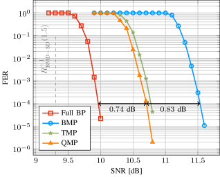
(a)

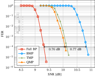
(b)

Figure 2: FER simulation results for uniform (a) and PAS (b) signaling and an SE of $1.5\text{\,}\mathrm{b}\mathrm{p}\mathrm{c}\mathrm{u}$.

VI Conclusion

Reducing the internal LDPC decoder data flow is essential for hardware implementations targeting application specific integrated circuits and constitutes an important prerequisite for high throughput decoders. In this work, we extensively compared one and two bit quantized BP decoding algorithms for higher order modulation and PS. For this, we also introduced a novel two-bit message passing decoding algorithm with a four-ary message alphabet that improves upon the previous TMP approach by up to $0.24\text{\,}\mathrm{d}\mathrm{B}$ for low code rates while having the same internal decoder dataflow. We showed how DE must be modified for the quantized message passing algorithms to account for higher order modulation and PS. The results were applied to protograph-based SC-LDPC codes to show the potential of the decoding algorithms for high throughput optical FEC solutions. Finite length simulation results reflected the predicted gains by DE.

Appendix A Scaling of CN Messages

We motivate the scaling of CN messages with the scaling factor $w$. Consider transmission of a binary symbol $x$ over two channels with transition probabilities $P_{Y_{1}|X}$ and $P_{Y_{2}|X}$. Upon observing $y_{1}$ and $y_{2}$, in order to perform a maximum likelihood decision we may compute

$$l(y_{1},y_{2})=\underbrace{\log\frac{P_{Y_{1}|X}(y_{1}|0)}{P_{Y_{1}|X}(y_{1}|1)}}_{l_{1}(y_{1})}+\underbrace{\log\frac{P_{Y_{2}|X}(y_{2}|0)}{P_{Y_{2}|X}(y_{2}|1)}}_{l_{2}(y_{2})}.$$ (51)

We apply the same principle at each VN processor. Thus, let the first channel be the communication channel for which $l_{1}$ is available. A message sent from a CN to a VN can be modeled as the observation of the RV $X$ after transmission over a binary-input $M$-ary output discrete memoryless extrinsic channel [40]. For an observation $y_{2}$, $l_{2}$ is computed from the transition probabilities of the extrinsic channel, for which accurate estimates can obtained by DE in the large block length regime.

Consider QMP as an example. The $4$-ary extrinsic channel output alphabet is $\mathcal{Y}=\{\pm\mathtt{H},\pm\mathtt{L}\}$, and we have

$$l_{2}(y)=\begin{cases}\log\frac{P_{Y_{2}|X}(\mathtt{H}|0)}{P_{Y_{2}|X}(\mathtt{H}|1)},&y=\mathtt{H}\\ \log\frac{P_{Y_{2}|X}(-\mathtt{H}|0)}{P_{Y_{2}|X}(-\mathtt{H}|1)},&y=-\mathtt{H}\\ \log\frac{P_{Y_{2}|X}(\mathtt{L}|0)}{P_{Y_{2}|X}(\mathtt{L}|1)},&y=\mathtt{L}\\ \log\frac{P_{Y_{2}|X}(-\mathtt{L}|0)}{P_{Y_{2}|X}(-\mathtt{L}|1)},&y=-\mathtt{L}.\end{cases}$$ (52)

Similarly to (14), we require that the extrinsic channel fulfills the symmetry constraint

$$P_{Y_{2}|X}(\mathtt{H}|0)=P_{Y_{2}|X}(-\mathtt{H}|1)$$ (53)

$$P_{Y_{2}|X}(\mathtt{L}|0)=P_{Y_{2}|X}(-\mathtt{L}|1).$$ (54)

Thus, we have

$$|l_{2}(y)|=\begin{cases}\log\frac{P_{Y_{2}|X}(\mathtt{H}|0)}{P_{Y_{2}|X}(\mathtt{H}|1)},&y=\pm\mathtt{H}\\ \log\frac{P_{Y_{2}|X}(\mathtt{L}|0)}{P_{Y_{2}|X}(\mathtt{L}|1)},&y=\pm\mathtt{L}.\end{cases}$$ (55)

Above, we assumed that $P_{Y_{2}|X}(\mathtt{H}|0)>P_{Y_{2}|X}(\mathtt{H}|1)$ and $P_{Y_{2}|X}(\mathtt{L}|0)>P_{Y_{2}|X}(\mathtt{L}|1)$. We have

$$l(y)=l_{1}+\operatorname*{sign}(y)|l_{2}(y)|.$$ (56)

As in (56), the VN update in Algorithm 2 performs a weighting of the extrinsic CN messages. Observe that the weighting factor $w$ in (32) and (33) is defined as $|l_{2}(y)|$ in (55).

References

• [1] A. Schmitt, “OFC 2018: Post-Show Report,” https://www.ofcconference.org/library/images/ofc/2018/Documents/OFC-2018-Show-Report.pdf.
• [2] B. P. Smith, A. Farhood, A. Hunt, F. R. Kschischang, and J. Lodge, “Staircase Codes: FEC for 100 Gb/s OTN,” J. Lightw. Technol., vol. 30, no. 1, pp. 110–117, Jan. 2012.
• [3] A. J. Feltstrom, D. Truhachev, M. Lentmaier, and K. S. Zigangirov, “Braided Block Codes,” IEEE Trans. Inf. Theory, vol. 55, no. 6, pp. 2640–2658, Jun. 2009.
• [4] M. Magarini, R. Essiambre, B. E. Basch, A. Ashikhmin, G. Kramer, and A. J. de Lind van Wijngaarden, “Concatenated Coded Modulation for Optical Communications Systems,” IEEE Photon. Technol. Lett., vol. 22, no. 16, pp. 1244–1246, Aug. 2010.
• [5] L. M. Zhang and F. R. Kschischang, “Low-Complexity Soft-Decision Concatenated LDGM-Staircase FEC for High-Bit-Rate Fiber-Optic Communication,” J. Lightw. Technol., vol. 35, no. 18, pp. 3991–3999, Sep. 2017.
• [6] A. Sheikh, A. Graell i Amat, and G. Liva, “Binary Message Passing Decoding of Product-like Codes,” arXiv:1902.03575 [cs, math], Feb. 2019, submitted to IEEE Trans. Commun.
• [7] G. Liga, A. Sheikh, and A. Alvarado, “A novel soft-aided bit-marking decoder for product codes,” arXiv:1906.09792 [cs, eess, math], Jun. 2019.
• [8] Y. Lei, B. Chen, G. Liga, X. Deng, Z. Cao, J. Li, K. Xu, and A. Alvarado, “Improved Decoding of Staircase Codes: The Soft-aided Bit-marking (SABM) Algorithm,” arXiv:1902.01178 [eess], Feb. 2019.
• [9] G. Lechner, T. Pedersen, and G. Kramer, “Analysis and Design of Binary Message Passing Decoders,” IEEE Trans. Commun., vol. 60, no. 3, pp. 601–607, Mar. 2012.
• [10] R. G. Gallager, “Low-Density Parity-Check Codes,” IRE Trans. Inf. Theory, vol. 8, no. 1, pp. 21–28, 1962.
• [11] P. Schläfer, N. Wehn, M. Alles, and T. Lehnigk-Emden, “A new dimension of parallelism in ultra high throughput LDPC decoding,” in Proc. Signal Process. Syst. (SiPS), Oct. 2013, pp. 153–158.
• [12] E. Ben Yacoub, F. Steiner, B. Matuz, and G. Liva, “Protograph-Based LDPC Code Design for Ternary Message Passing Decoding,” in Proc. Int. ITG Conf. Syst. Commun. Coding (SCC), Rostock, Germany, Feb. 2019.
• [13] T. J. Richardson and R. L. Urbanke, “The Capacity of Low-Density Parity-Check Codes under Message-Passing Decoding,” IEEE Trans. Inf. Theory, vol. 47, no. 2, pp. 599–618, 2001.
• [14] G. Böcherer, F. Steiner, and P. Schulte, “Bandwidth Efficient and Rate-Matched Low-Density Parity-Check Coded Modulation,” IEEE Trans. Commun., vol. 63, no. 12, pp. 4651–4665, Dec. 2015.
• [15] G. Böcherer, P. Schulte, and F. Steiner, “Probabilistic Shaping and Forward Error Correction for Fiber-Optic Communication Systems,” J. Lightw. Technol., vol. 37, no. 2, pp. 230–244, Jan. 2019.
• [16] P. Poggiolini, G. Bosco, A. Carena, V. Curri, Y. Jiang, and F. Forghieri, “The GN-Model of Fiber Non-Linear Propagation and its Applications,” J. Lightw. Technol., vol. 32, no. 4, pp. 694–721, Feb. 2014.
• [17] C. E. Shannon, “A Mathematical Theory of Communication,” Bell Syst. Tech. J., vol. 27, no. 3, pp. 379–423, Jul. 1948.
• [18] R. G. Gallager, Information Theory and Reliable Communication.   John Wiley & Sons, Inc., 1968.
• [19] G. D. Forney, “Trellis Shaping,” IEEE Trans. Inf. Theory, vol. 38, no. 2, pp. 281–300, Mar. 1992.
• [20] P. Schulte and G. Böcherer, “Constant Composition Distribution Matching,” IEEE Trans. Inf. Theory, vol. 62, no. 1, pp. 430–434, Jan. 2016.
• [21] W. G. Bliss, “Circuitry for Performing Error Correction Calculations on Baseband Encoded Data to Eliminate Error Propagation,” IBM Techn. Discl. Bull., no. 23, Mar. 1981.
• [22] M. Mansuripur, “Enumerative Modulation Coding with Arbitrary Constraints and Post-modulation Error Correction Coding for Data Storage Systems,” in Proc. SPIE Conf. Optical Data Storage, vol. 1499, Colorado Springs, CO, Feb. 1991.
• [23] G. Böcherer, “Principles of Coded Modulation,” habilitation thesis, Technical University of Munich, 2018. [Online]. Available: http://www.georg-boecherer.de/bocherer2018principles.pdf
• [24] R. A. Amjad, “Information Rates and Error Exponents for Probabilistic Amplitude Shaping,” in Proc. IEEE Inf. Theory Workshop (ITW), Guangzhou, China, Nov. 2018.
• [25] J. Cho and P. J. Winzer, “Probabilistic Constellation Shaping for Optical Fiber Communications,” J. Lightw. Technol., vol. 37, no. 6, pp. 1590–1607, Mar. 2019.
• [26] T. Richardson and R. Urbanke, “Multi-Edge Type LDPC Codes,” Workshop honoring Prof. Bob McEliece on his 60th birthday, California Institute of Technology, Pasadena, California, pp. 24–25, 2002.
• [27] J. Thorpe, “Low-Density Parity-Check (LDPC) Codes Constructed from Protographs,” IPN progress report, vol. 42, no. 154, pp. 42–154, 2003.
• [28] D. Divsalar, S. Dolinar, C. R. Jones, and K. Andrews, “Capacity-Approaching Protograph Codes,” IEEE J. Sel. Areas Commun., vol. 27, no. 6, pp. 876–888, Aug. 2009.
• [29] L. Schmalen, V. Aref, J. Cho, D. Suikat, D. Rösener, and A. Leven, “Spatially Coupled Soft-Decision Error Correction for Future Lightwave Systems,” J. Lightw. Technol., vol. 33, no. 5, pp. 1109–1116, Mar. 2015.
• [30] A. R. Iyengar, P. H. Siegel, R. L. Urbanke, and J. K. Wolf, “Windowed Decoding of Spatially Coupled Codes,” IEEE Trans. Inf. Theory, vol. 59, no. 4, pp. 2277–2292, Apr. 2013.
• [31] S. Kudekar, T. J. Richardson, and R. L. Urbanke, “Threshold Saturation via Spatial Coupling: Why Convolutional LDPC Ensembles Perform So Well over the BEC,” IEEE Trans. Inf. Theory, vol. 57, no. 2, pp. 803–834, Feb. 2011.
• [32] J. Hou, P. H. Siegel, L. B. Milstein, and H. D. Pfister, “Capacity-Approaching Bandwidth-Efficient Coded Modulation Schemes Based on Low-Density Parity-Check Codes,” IEEE Trans. Inf. Theory, vol. 49, no. 9, pp. 2141–2155, Sep. 2003.
• [33] C. Fougstedt, A. Sheikh, A. Graell i Amat, G. Liva, and P. Larsson-Edefors, “Energy-Efficient Soft-Assisted Product Decoders,” in Proc. Optical Fiber Commun. Conf. (OFC), Mar. 2019, paper W3H.6.
• [34] F. Peng, W. Ryan, and R. Wesel, “Surrogate-Channel Design of Universal LDPC Codes,” IEEE Commun. Lett., vol. 10, no. 6, pp. 480–482, Jun. 2006.
• [35] M. Franceschini, G. Ferrari, and R. Raheli, “Does the Performance of LDPC Codes Depend on the Channel?” IEEE Trans. Commun., vol. 54, no. 12, pp. 2129–2132, Dec. 2006.
• [36] I. Sason, “On Universal Properties of Capacity-Approaching LDPC Code Ensembles,” IEEE Trans. Inf. Theory, vol. 55, no. 7, pp. 2956–2990, Jul. 2009.
• [37] A. R. Iyengar, M. Papaleo, P. H. Siegel, J. K. Wolf, A. Vanelli-Coralli, and G. E. Corazza, “Windowed Decoding of Protograph-Based LDPC Convolutional Codes Over Erasure Channels,” IEEE Trans. Inf. Theory, vol. 58, no. 4, pp. 2303–2320, Apr. 2012.
• [38] S.-Y. Chung, G. D. Forney, T. J. Richardson, and R. Urbanke, “On the Design of Low-Density Parity-Check Codes within 0.0045 dB of the Shannon Limit,” IEEE Commun. Lett., vol. 5, no. 2, pp. 58–60, 2001.
• [39] F. Kschischang and S. Pasupathy, “Optimal Nonuniform Signaling for Gaussian Channels,” IEEE Trans. Inf. Theory, vol. 39, no. 3, pp. 913–929, May 1993.
• [40] A. Ashikhmin, G. Kramer, and S. ten Brink, “Extrinsic Information Transfer Functions: Model and Erasure Channel Properties,” IEEE Trans. Inf. Theory, vol. 50, no. 11, pp. 2657–2673, 2004.