Abstract

Kernels are powerful and versatile tools in machine learning and statistics. Although the notion of universal kernels and characteristic kernels has been studied, kernel selection still greatly influences the empirical performance. While learning the kernel in a data driven way has been investigated, in this paper we explore learning the spectral distribution of kernel via implicit generative models parametrized by deep neural networks. We called our method Implicit Kernel Learning (IKL). The proposed framework is simple to train and inference is performed via sampling random Fourier features. We investigate two applications of the proposed IKL as examples, including generative adversarial networks with MMD (MMD GAN) and standard supervised learning. Empirically, MMD GAN with IKL outperforms vanilla predefined kernels on both image and text generation benchmarks; using IKL with Random Kitchen Sinks also leads to substantial improvement over existing state-of-the-art kernel learning algorithms on popular supervised learning benchmarks. Theory and conditions for using IKL in both applications are also studied as well as connections to previous state-of-the-art methods.

1 Introduction

Kernel methods are among the essential foundations in machine learning and have been extensively studied in the past decades. In supervised learning, kernel methods allow us to learn non-linear hypothesis. They also play a crucial role in statistics. Kernel maximum mean discrepancy (MMD) (Gretton et al.,, 2012) is a powerful two-sample test, which is based on a statistics computed via kernel functions. Even though there is a surge of deep learning in the past years, several successes have been shown by kernel methods and deep feature extraction. Wilson et al., (2016) demonstrate state-of-the-art performance by incorporating deep learning, kernel and Gaussian process. Li et al., (2015); Dziugaite et al., (2015) use MMD to train deep generative models for complex datasets.

In practice, however, kernel selection is always an important step. Instead of choosing by a heuristic, several works have studied kernel learning. Multiple kernel learning (MKL) (Bach et al.,, 2004; Lanckriet et al.,, 2004; Bach,, 2009; Gönen and Alpaydın,, 2011; Duvenaud et al.,, 2013) is one of the pioneering frameworks to combine predefined kernels. One recent kernel learning development is to learn kernels via learning spectral distributions (Fourier transform of the kernel). Wilson and Adams, (2013) model spectral distributions via a mixture of Gaussians, which can also be treated as an extension of linear combination of kernels (Bach et al.,, 2004). Oliva et al., (2016) extend it to Bayesian non-parametric models. In addition to model spectral distribution with explicit density models aforementioned, many works optimize the sampled random features or its weights (e.g. Băzăvan et al., (2012); Yang et al., (2015); Sinha and Duchi, (2016); Chang et al., (2017); Bullins et al., (2018)). The other orthogonal approach to modeling spectral distributions is learning feature maps for standard kernels (e.g. Gaussian). Feature maps learned by deep learning lead to state-of-the-art performance on different tasks (Hinton and Salakhutdinov,, 2008; Wilson et al.,, 2016; Li et al.,, 2017).

In addition to learning effective features, implicit generative models via deep learning also lead to promising performance in learning distributions of complex data (Goodfellow et al.,, 2014). Inspired by its recent success, we propose to model kernel spectral distributions with implicit generative models in a data-driven fashion, which we call Implicit Kernel Learning (IKL). IKL provides a new route to modeling spectral distributions by learning sampling processes of the spectral densities, which is under explored by previous works aforementioned.

In this paper, we start from studying the generic problem formulation of IKL, and propose an easily implemented, trained and evaluated neural network parameterization which satisfies Bochner’s theorem (Section 2). We then demonstrate two example applications of the proposed IKL. Firstly, we explore MMD GAN (Li et al.,, 2017) with IKL on learning to generate images and text (Section 3). Secondly, we consider a standard two-staged supervised learning task with Random Kitchen Sinks (Sinha and Duchi,, 2016) (Section 4). The conditions required for training IKL and its theoretical guarantees in both tasks are also studied. In both tasks, we show that IKL leads to competitive or better performance than heuristic kernel selections and existing approaches modeling kernel spectral densities. It demonstrates the potentials of learning more powerful kernels via deep generative models. Finally, we discuss the connection with existing works in Section 5.

2 Kernel Learning

Kernels have been used in several applications with success, including supervised learning, unsupervised learning, and hypothesis testing. They have also been combined with deep learning in different applications (Mairal et al.,, 2014; Li et al.,, 2015; Dziugaite et al.,, 2015; Wilson et al.,, 2016; Mairal,, 2016). Given data $x\in\mathbb{R}^{d}$, kernel methods compute the inner product of the feature transformation $\phi(x)$ in a high-dimensional Hilbert space $H$ via a kernel function $k:\mathcal{X}\times\mathcal{X}\rightarrow\mathbb{R}$, which is defined as $k(x,x^{\prime})=\langle\phi(x),\phi(x^{\prime})\rangle_{H}$, where $\phi(x)$ is usually high or even infinitely dimensional. If $k$ is shift invariant (i.e. $k(x,y)=k(x-y)$), we can represent $k$ as an expectation with respect to a spectral distribution $\mathbb{P}_{k}(\omega)$.

Bochner’s theorem (Rudin,, 2011)

A continuous, real valued, symmetric and shift-invariant function $k$ on $\mathbb{R}^{d}$ is a positive definite kernel if and only if there is a positive finite measure $\mathbb{P}_{k}(\omega)$ such that

$$k(x-x^{\prime})=\int_{\mathbb{R}^{d}}e^{i\omega^{\top}(x-x^{\prime})}d\mathbb{P}_{k}(\omega)=\mathbb{E}_{\omega\sim\mathbb{P}_{k}}\left[e^{i\omega^{\top}(x-x^{\prime})}\right].$$

2.1 Implicit Kernel Learning

We restrict ourselves to learning shift invariant kernels. According to that, learning kernels is equivalent to learning a spectral distribution by optimizing

$$\begin{array}[]{l}\displaystyle\arg\max_{k\in\mathcal{K}}\sum_{i=1}\mathbb{E}_{x\sim\mathbb{P}_{i},x^{\prime}\sim\mathbb{Q}_{i}}\left[F_{i}(x,x^{\prime})k(x,x^{\prime})\right]=\\ \displaystyle\arg\max_{k\in\mathcal{K}}\sum_{i=1}\mathbb{E}_{x\sim\mathbb{P}_{i},x^{\prime}\sim\mathbb{Q}_{i}}\left[F_{i}(x,x^{\prime})\mathbb{E}_{\omega\sim\mathbb{P}_{k}}\left[e^{i\omega^{\top}(x-x^{\prime})}\right]\right],\end{array}$$ (1)

where $F$ is a task-specific objective function and $\mathcal{K}$ is a set of kernels. (1) covers many popular objectives, such as kernel alignment (Gönen and Alpaydın,, 2011) and MMD distance (Gretton et al.,, 2012). Existing works (Wilson and Adams,, 2013; Oliva et al.,, 2016) learn the spectral density $\mathbb{P}_{k}(\omega)$ with explicit forms via parametric or non-parametric models. When we learn kernels via (1), it may not be necessary to model the density of $\mathbb{P}_{k}(\omega)$, as long as we are able to estimate kernel evaluations $k(x-x^{\prime})=\mathbb{E}_{\omega}[e^{i\omega^{\top}(x-x^{\prime})}]$ via sampling from $\mathbb{P}_{k}(\omega)$ (Rahimi and Recht,, 2007). Alternatively, implicit probabilistic (generative) models define a stochastic procedure that can generate (sample) data from $\mathbb{P}_{k}(\omega)$ without modeling $\mathbb{P}_{k}(\omega)$. Recently, the neural implicit generative models (MacKay,, 1995) regained attentions with promising results (Goodfellow et al.,, 2014) and simple sampling procedures. We first sample $\nu$ from a base distribution $\mathbb{P}(\nu)$ which is known (e.g. Gaussian distribution), then use a deterministic function $h_{\psi}$ parametrized by $\psi$, to transform $\nu$ into $\omega=h_{\psi}(\nu)$, where $\omega$ follows the complex target distribution $\mathbb{P}_{k}(\omega)$. Inspired by the success of deep implicit generative models (Goodfellow et al.,, 2014), we propose an Implicit Kernel Learning (IKL) method by modeling $\mathbb{P}_{k}(\omega)$ via an implicit generative model $h_{\psi}(\nu)$, where $\nu\sim\mathbb{P}(\nu)$, which results in

$$k_{\psi}(x,x^{\prime})=\mathbb{E}_{\nu}\left[e^{ih_{\psi}(\nu)^{\top}(x-x^{\prime})}\right]$$ (2)

and reducing (1) to solve

$$\begin{array}[]{c}\displaystyle\arg\max_{\psi}\sum_{i=1}\mathbb{E}_{x\sim\mathbb{P}_{i},x^{\prime}\sim\mathbb{Q}_{i}}\left[F_{i}(x,x^{\prime})\mathbb{E}_{\nu}\left(e^{ih_{\psi}(\nu)^{\top}(x-x^{\prime})}\right)\right].\\ \end{array}$$ (3)

The gradient of  (3) can be represented as

$$\sum_{i=1}\mathbb{E}_{x\sim\mathbb{P}_{i},x^{\prime}\sim\mathbb{Q}_{i}}\mathbb{E}_{\nu}\left[\nabla_{\psi}F_{i}(x,x^{\prime})e^{ih_{\psi}(\nu)^{\top}(x-x^{\prime})}\right].$$

Thus,  (3) can be optimized via sampling $x,x^{\prime}$ from data and $\nu$ from the base distribution to estimate gradient as shown above (SGD) in every iteration. Next, we discuss the parametrization of $h_{\psi}$ to satisfy Bochner’s Theorem, and describe how to evaluate IKL kernel in practice.

Symmetric $\mathbb{P}_{k}(\omega)$

To result in real valued kernels, the spectral density has to be symmetric, where $\mathbb{P}_{k}(\omega)=\mathbb{P}_{k}(-\omega)$. Thus, we parametrize $h_{\psi}(\nu)=\mbox{{sign}}(\nu)\circ\tilde{h}_{\psi}(\mbox{{abs}}(\nu))$, where $\circ$ is the Hadamard product and $\tilde{h}_{\psi}$ can be any unconstrained function if the base distribution $\mathbb{P}(\nu)$ is symmetric (i.e. $\mathbb{P}(\nu)=\mathbb{P}(-\nu)$), such as standard normal distributions.

Kernel Evaluation

Although there is usually no closed form for the kernel evaluation $k_{\psi}(x,x^{\prime})$ in (2) with fairly complicated $h_{\psi}$, we can evaluate (approximate) $k_{\psi}(x,x^{\prime})$ via sampling finite number of random Fourier features $\hat{k}_{\psi}(x,x^{\prime})=\hat{\phi}_{h_{\psi}}(x)^{\top}\hat{\phi}_{h_{\psi}}(x^{\prime})$, where $\hat{\phi}_{h_{\psi}}(x)^{\top}=[\phi(x;h_{\psi}(\nu_{1})),\dots,\phi(x;h_{\psi}(\nu_{m}))]$, and $\phi(x;\omega)$ is the evaluation on $\omega$ of the Fourier transformation $\phi(x)$ (Rahimi and Recht,, 2007).

Next, we demonstrate two example applications covered by (3), where we can apply IKL, including kernel alignment and maximum mean discrepancy (MMD).

3 MMD GAN with IKL

Given $\{x_{i}\}_{i=1}^{n}\sim\mathbb{P}_{\mathcal{X}}$, instead of estimating the density $\mathbb{P}_{\mathcal{X}}$, Generative Adversarial Network (GAN) (Goodfellow et al.,, 2014) is an implicit generative model, which learns a generative network $g_{\theta}$ (generator). The generator $g_{\theta}$ transforms a base distribution $\mathbb{P}_{\mathcal{Z}}$ over $\mathcal{Z}$ into $\mathbb{P}_{\theta}$ to approximate $\mathbb{P}_{\mathcal{X}}$, where $\mathbb{P}_{\theta}$ is the distribution of $g_{\theta}(z)$ and $z\sim\mathbb{P}_{\mathcal{Z}}$. During the training, GAN alternatively estimates a distance $D(\mathbb{P}_{\mathcal{X}}\|\mathbb{P}_{\theta})$ between $\mathbb{P}_{\mathcal{X}}$ and $\mathbb{P}_{\theta}$, and updates $g_{\theta}$ to minimize $D(\mathbb{P}_{\mathcal{X}}\|\mathbb{P}_{\theta})$. Different probability metrics have been studied (Goodfellow et al.,, 2014; Li et al.,, 2015; Dziugaite et al.,, 2015; Nowozin et al.,, 2016; Arjovsky et al.,, 2017; Mroueh et al.,, 2017; Li et al.,, 2017; Mroueh and Sercu,, 2017; Gulrajani et al.,, 2017; Mroueh et al.,, 2018; Arbel et al.,, 2018) for training GANs.

Kernel maximum mean discrepancy (MMD) is a probability metric, which is commonly used in two-sample-test to distinguish two distributions with finite samples (Gretton et al.,, 2012). Given a kernel $k$, the MMD between $\mathbb{P}$ and $\mathbb{Q}$ is defined as

$$M_{k}(\mathbb{P},\mathbb{Q})=\mathbb{E}_{\mathbb{P},\mathbb{P}}[k(x,x^{\prime})]-2\mathbb{E}_{\mathbb{P},\mathbb{Q}}[k(x,y)]+\mathbb{E}_{\mathbb{Q},\mathbb{Q}}[k(y,y^{\prime})].$$ (4)

For characteristic kernels, $M_{k}(\mathbb{P},\mathbb{Q})=0$ iff $\mathbb{P}=\mathbb{Q}$. Li et al., (2015); Dziugaite et al., (2015) train the generator $g_{\theta}$ by optimizing $\min_{\theta}{M}_{k}(\mathbb{P}_{\mathcal{X}},\mathbb{P}_{\theta})$ with a Gaussian kernel $k$. Li et al., (2017) propose MMD GAN, which trains $g_{\theta}$ via $\min_{\theta}\max_{k\in\mathcal{K}}{M}_{k}(\mathbb{P}_{\mathcal{X}},\mathbb{P}_{\theta})$, where $\mathcal{K}$ is a pre-defined set of kernels. The intuition is to learn a kernel $\mathop{\mathrm{argmax}}_{k\in\mathcal{K}}{M}_{k}(\mathbb{P}_{\mathcal{X}},\mathbb{P}_{\theta})$, which has a stronger signal (i.e. larger distance when $\mathbb{P}_{\mathcal{X}}\neq\mathbb{P}_{\theta}$) to train $g_{\theta}$. Specifically, Li et al., (2017) consider a composition kernel $k_{\varphi}$ which combines Gaussian kernel $k$ and a neural network $f_{\varphi}$ as $k_{\varphi}=k\circ f_{\varphi}$, where

$$k_{\varphi}(x,x^{\prime})=\exp(-\|f_{\varphi}(x)-f_{\varphi}(x)^{\prime}\|^{2}).$$ (5)

The MMD GAN objective then becomes $\min_{\theta}\max_{\varphi}M_{\varphi}(\mathbb{P}_{\mathcal{X}},\mathbb{P}_{\theta})$.

3.1 Training MMD GAN with IKL

Although the composition kernel with a learned feature embedding $f_{\varphi}$ is powerful, choosing a good base kernel $k$ is still crucial in practice (Bińkowski et al.,, 2018). Different base kernels for MMD GAN, such as rational quadratic kernel (Bińkowski et al.,, 2018) and distance kernel (Bellemare et al.,, 2017), have been studied. Instead of choosing it by hands, we propose to learn the base kernel by IKL, which extend (5) to be $k_{\psi,\varphi}=k_{\psi}\circ f_{\varphi}$ with the form

$$k_{\psi,\varphi}(x,x^{\prime})=\mathbb{E}_{\nu}\left[e^{ih_{\psi}(\nu)^{\top}(f_{\varphi}(x)-f_{\varphi}(x^{\prime}))}\right].$$ (6)

We then extend the MMD GAN objective to be

$$\min_{\theta}\max_{\psi,\varphi}M_{\psi,\varphi}(\mathbb{P}_{\mathcal{X}},\mathbb{P}_{\theta}),$$ (7)

where $M_{\psi,\varphi}$ is the MMD distance (4) with the IKL kernel (6). Clearly, for a given $\varphi$, the maximization over $\psi$ in (7) can be represented as (1) by letting $F_{1}(x,x^{\prime})=1$, $F_{2}(x,y)=-2$ and $F_{3}(y,y^{\prime})=1$. In what follows, we will use for convenience $k_{\psi,\varphi}$, $k_{\psi}$ and $k_{\varphi}$ to denote kernels defined in (6), (2) and  (5) respectively.

3.2 Property of MMD GAN with IKL

As proven by Arjovsky and Bottou, (2017), some probability distances adopted by existing works (e.g. Goodfellow et al., (2014)) are not weak (i.e. $\mathbb{P}_{n}\xrightarrow[]{D}\mathbb{P}$ then $D(\mathbb{P}_{n}\|\mathbb{P})\rightarrow 0$), which cannot provide better signal to train $g_{\theta}$. Also, they usually suffer from discontinuity, hence it cannot be trained via gradient descent at certain points. We prove that $\max_{\psi,\varphi}M_{\psi,\varphi}(\mathbb{P}_{\mathcal{X}},\mathbb{P}_{\theta})$ is a continuous and differentiable objective in $\theta$ and weak under mild assumptions as used in (Arjovsky et al.,, 2017; Li et al.,, 2017).

Assumption 1.

$g_{\theta}(z)$ is locally Lipschitz and differentiable in $\theta$; $f_{\varphi}(x)$ is Lipschitz in $x$ and $\varphi\in\Phi$ is compact. $f_{\varphi}\circ g_{\theta}(z)$ is differentiable in $\theta$ and there are local Lipschitz constants, which is independent of $\varphi$, such that $\mathbb{E}_{z\sim\mathbb{P}_{z}}[L(\theta,z)]<+\infty$. The above assumptions are adopted by Arjovsky et al., (2017). Lastly, assume given any $\psi\in\Psi$, where $\Psi$ is compact, $k_{\psi}(x,x^{\prime})=\mathbb{E}_{\nu}\left[e^{ih_{\psi}(\nu)^{\top}(x-x^{\prime})}\right]$ and $|k_{\psi}(x,x^{\prime})|<\infty$ is differentiable and Lipschitz in $(x,x^{\prime})$ which has an upper bound $L_{k}$ for Lipschitz constant of $(x,x^{\prime})$ given different $\psi$.

Theorem 2.

Assume function $g_{\theta}$ and kernel $k_{\psi,\varphi}$ satisfy Assumption 1, $\max_{\psi,\varphi}M_{\psi,\varphi}$ is weak, that is, $\max_{\psi,\varphi}M_{\psi,\varphi}(\mathbb{P}_{\mathcal{X}},\mathbb{P}_{n})\rightarrow 0\Longleftrightarrow\mathbb{P}_{n}\xrightarrow[]{D}\mathbb{P}_{\mathcal{X}}$. Also, $\max_{\psi,\varphi}M_{\psi,\varphi}(\mathbb{P}_{\mathcal{X}},\mathbb{P}_{\theta})$ is continuous everywhere and differentiable almost everywhere in $\theta$.

Lemma 3.

Assume $\mathcal{X}$ is bounded. Let $x,x^{\prime}\in\mathcal{X}$, $k_{\psi}(x,x^{\prime})=\mathbb{E}_{\nu}\left[e^{ih_{\psi}(\nu)^{\top}(x-x^{\prime})}\right]$ is Lipschitz in $(x,x^{\prime})$ if $\mathbb{E}_{\nu}\left[\|h_{\psi}(\nu)\|^{2}\right]<\infty$, which is variance since $\mathbb{E}_{\nu}\left[h_{\psi}(\nu)\right]=0.$

We penalize $\lambda_{h}(\mathbb{E}_{\nu}\left[\|h_{\psi}(\nu)\|^{2}\right]-u)^{2}$ as an approximation of Lemma 3 in practice to ensure that assumptions in Theorem 2 are satisfied. The algorithm with IKL and gradient penalty (Bińkowski et al.,, 2018) is shown in Algorithm 1.

  Input: $\eta$ the learning rate, $B$ the batch size, $n_{c}$ number of $f,h$ updates per $g$ update, $m$ the number of basis, $\lambda_{GP}$ the coefficient of gradient penalty, $\lambda_{h}$ the coefficient of variance constraint.

  Initial parameter $\theta$ for $g$, $\varphi$ for $f$, $\psi$ for $h$

  Define $\mathcal{L}(\psi,\varphi)=M_{\psi,\varphi}(\mathbb{P}_{\mathcal{X}},\mathbb{P}_{\theta})-\lambda_{GP}(\|\nabla_{\hat{x}}f_{\varphi}(\hat{x})\|_{2}-1)^{2}-\lambda_{h}(\mathbb{E}_{\nu}[\|h_{\psi}(\nu)\|^{2}]-u)^{2}$

  while $\theta$ has not converged do

     for $t=1,\ldots,n_{c}$ do

        Sample $\{x_{i}\}_{i=1}^{B}\sim\mathbb{P}(\mathcal{X}),\ \{z_{j}\}_{j=1}^{B}\sim\mathbb{P}(\mathcal{Z}),\ \{\nu_{k}\}_{k=1}^{m}\sim\mathbb{P}(\nu)$

         $(\psi,\varphi)\leftarrow\varphi+\eta\text{Adam}\left((\psi,\varphi),\nabla_{\psi,\varphi}\mathcal{L}(\psi,\varphi)\right)$

     end for

     Sample $\{x_{i}\}_{i=1}^{B}\sim\mathbb{P}(\mathcal{X}),\ \{z_{j}\}_{j=1}^{B}\sim\mathbb{P}(\mathcal{Z}),\ \{\nu_{k}\}_{k=1}^{m}\sim\mathbb{P}(\nu)$

      $\theta\leftarrow\theta-\eta\text{Adam}(\theta,\nabla_{\theta}M_{\psi,\varphi}(\mathbb{P}_{\mathcal{X}},\mathbb{P}_{\theta}))$

  end while

Algorithm 1 MMD GAN with IKL

3.3 Empirical Study

We consider image and text generation tasks for quantitative evaluation. For image generation, we evaluate the inception score (Salimans et al.,, 2016) and FID score (Heusel et al.,, 2017) on CIFAR-10 (Krizhevsky and Hinton,, 2009). We use DCGAN (Radford et al.,, 2016) and expands the output of $f_{\varphi}$ to be 16-dimensional as Bińkowski et al., (2018). For text generation, we consider a length-32 character-level generation task on Google Billion Words dataset. The evaluation is based on Jensen-Shannon divergence on empirical 4-gram probabilities (JS-4) of the generated sequence and the validation data as used by Gulrajani et al., (2017); Heusel et al., (2017); Mroueh et al., (2018). The model architecture follows Gulrajani et al., (2017) in using ResNet with 1D convolutions. We train every algorithm $10,000$ iterations for comparison.

For MMD GAN with fixed base kernels, we consider the mixture of Gaussian kernels $k(x,x^{\prime})=\sum_{q}\exp(-\frac{\|x-x^{\prime}\|^{2}}{2\sigma_{q}^{2}})$ (Li et al.,, 2017) and the mixture of RQ kernels $k(x,x^{\prime})=\sum_{q}(1+\frac{\|x-x^{\prime}\|^{2}}{2\alpha_{q}})^{-\alpha_{q}}$. We tuned hyperparameters $\sigma_{q}$ and $\alpha_{q}$ for each kernel as reported in Appendix F.1.

Lastly, for learning base kernels, we compare IKL with SM kernel (Wilson and Adams,, 2013) $f_{\varphi}$, which learns mixture of Gaussians to model kernel spectral density. It can also be treated as the explicit generative model counter part of the proposed IKL.

In both tasks, $\mathbb{P}(\nu)$, the base distribution of IKL, is a standard normal distribution and $h_{\psi}$ is a 3-layer MLP with $32$ hidden units for each layer. Similar to the aforementioned mixture kernels, we consider the mixture of IKL kernel with the variance constraints $\mathbb{E}[\|h_{\psi}(\nu)\|^{2}]=1/\sigma_{q}$, where $\sigma_{q}$ is the bandwidths for the mixture of Gaussian kernels. Note that if $h_{\psi}$ is an identity map, we recover the mixture of Gaussian kernels. We fix $\lambda_{h}$ to be $10$ and resample $m=1024$ random features for IKL in every iteration. For other settings, we follow Bińkowski et al., (2018) and the hyperparameters can be found in Appendix F.1.

3.3.1 Results and Discussion

We compare MMD GAN with the proposed IKL and different fixed kernels. We repeat the experiments $10$ times and report the average result with standard error in Table 1. Note that for inception score the larger the better; while JS-4 the smaller the better. We also report WGAN-GP results as a reference. Since FID score results (Heusel et al.,, 2017) is consistent with inception score and does not change our discussion, we put it in Appendix C.1 due to space limit. Sampled images on larger datasets are shown in Figure 1.

Method	Inception Scores $(\uparrow)$	JS-4 $(\downarrow)$
Gaussian	$6.726\pm 0.021$	$0.381\pm 0.003$
RQ	$6.785\pm 0.031$	$0.463\pm 0.005$
SM	$6.746\pm 0.031$	$0.378\pm 0.003$
IKL	$\mathbf{6.876\pm 0.018}$	$\mathbf{0.372\pm 0.002}$
WGAN-GP	$6.539\pm 0.034$	$0.379\pm 0.002$

Table 1: Inception scores and JS-4 divergece results.

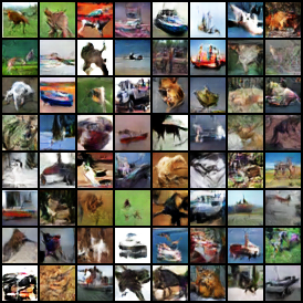
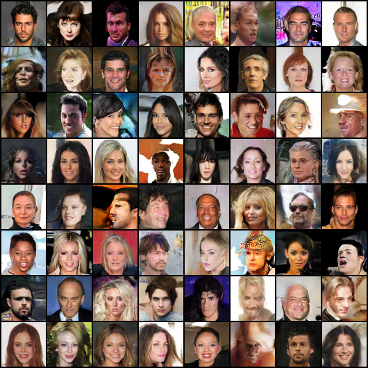
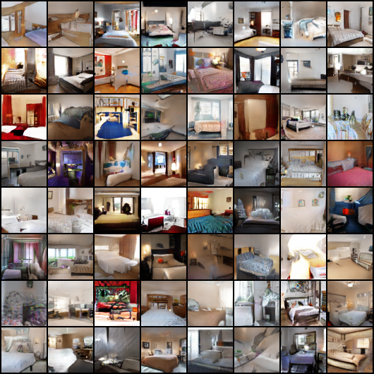
Figure 1: Samples generated by MMDGAN-IKL on CIFAR-10, CELEBA and LSUN dataset.

Pre-defined Kernels

Bińkowski et al., (2018) show RQ kernels outperform Gaussian and energy distance kernels on image generation. Our empirical results agree with such finding: RQ kernels achieve $6.785$ inception score while for Gaussian kernel it is $6.726$, as shown in the left column of Table 1. In text generation, nonetheless, RQ kernels only achieve $0.463$ JS-4 score and are not on par with $0.381$ acquired by Gaussian kernels, even though it is still slightly worse than WGAN-GP. These results imply kernel selection is task-specific. On the other hand, the proposed IKL learns kernels in a data-driven way, which results in the best performance in both tasks. In CIFAR-10, although Gaussian kernel is worse than RQ, IKL is still able to transforms $\mathbb{P}(\nu)$, which is Gaussian, into a powerful kernel, and outperforms RQ on inception scores ($6.876$ v.s. $6.785$). For text generation, from Table 1 and Figure 2, we observe that IKL can further boost Gaussian into better kernels with substantial improvement. Also, we note that the difference between IKL and pre-defined kernels in Table 1 is significant based on the $t$-test at 95% confidence level.

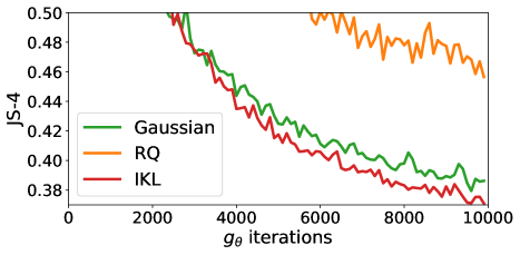
Figure 2: Convergence of MMD GANs with different kernels on text generation.

Learned Kernels

The SM kernel (Wilson and Adams,, 2013), which learns the spectral density via mixture of Gaussians, does not significantly outperforms Gaussian kernel as shown in Table 1, since  Li et al., (2017) already uses equal-weighted mixture of Gaussian formulation. It suggests that proposed IKL can learn more complicated and effective spectral distributions than simple mixture models.

Study of Variance Constraints

In Lemma 3, we prove bounding variance $\mathbb{E}[\|h_{\psi}(\nu)\|^{2}]$ guarantees $k_{\psi}$ to be Lipschitz as required in Theorem 2. We investigate the importance of this constraint. In Figure 3, we show the training objective (MMD), $\mathbb{E}[\|h_{\psi}(\nu)\|^{2}]$ and the JS-4 divergence for training MMD GAN (IKL) without variance constraint, i.e. $\lambda_{h}=0$. We could observe the variance keeps going up without constraints, which leads exploded MMD values. Also, when the exploration is getting severe, the JS-4 divergence starts increasing, which implies MMD cannot provide meaningful signal to $g_{\theta}$. The study justifies the validity of Theorem 2 and Lemma 3.

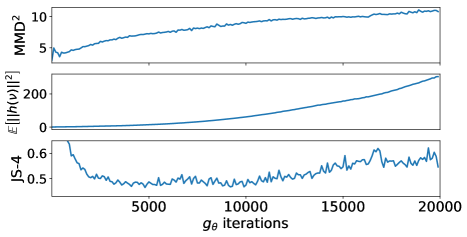
Figure 3: Learning MMD GAN (IKL) without the variance constraint on Google Billion Words datasets for text generation.

Other Studies

One concern of the proposed IKL is the computational overhead introduced by sampling random features as well as using more parameters to model $h_{\psi}$. Since we only use small network to model $h_{\psi}$, the increased computation overhead is almost negligible under GPU parallel computation. The detailed comparison can be found in Appendix C.2. We also compare IKL with Bullins et al., (2018), which can be seen as a variant of IKL without $h_{\psi}$, and studt the variance constraint. Those additional discussions can be found in Appendix C.1.

4 Random Kitchen Sinks with IKL

Rahimi and Recht, (2009) propose Random Kitchen Sinks (RKS) as follows. We sample $\omega_{i}\sim\mathbb{P}_{k}(\omega)$ and transform $x\in\mathbb{R}^{d}$ into $\hat{\phi}(x)=[\phi(x;\omega_{1}),\dots,\phi(x;\omega_{M})]$, where $\sup_{x,\omega}|\phi(x;\omega)|<1$. We then learn a classifier on the transformed features $\hat{\phi}(x;\omega)$. Kernel methods with random features (Rahimi and Recht,, 2007) is an example of RKS, where $\mathbb{P}_{k}(\omega)$ is the spectral distribution of the kernel and $\phi(x;\omega)=\big{[}\cos(\omega^{\top}x),\sin(\omega^{\top}x)\big{]}$. We usually learn a model $\mathbf{w}$ by solving

$$\arg\min_{\mathbf{w}}\frac{\lambda}{2}\|\mathbf{w}\|^{2}+\frac{1}{n}\sum_{i=1}^{n}\ell\left(\mathbf{w}^{\top}\hat{\phi}(x_{i})\right).$$ (8)

If $\ell$ is a convex loss function, the objective (8) can be solved efficiently to global optimum.

Spectral distributions $\mathbb{P}_{k}$ are usually set as a parameterized form, such as Gaussian distributions, but the selection of $\mathbb{P}_{k}$ is important in practice. If we consider RKS as kernel methods with random features, then selecting $\mathbb{P}$ is equivalent to the well-known kernel selection (learning) problem for supervised learning (Gönen and Alpaydın,, 2011).

Two-Stage Approach

We follows Sinha and Duchi, (2016) to consider kernel learning for RKS with a two-stage approach. In stage 1, we consider kernel alignment (Cristianini et al.,, 2002) of the form, $\mathop{\mathrm{argmax}}_{k\in\mathcal{K}}\mathbb{E}_{(x,y),(x^{\prime},y^{\prime})}\sum_{i\neq j}yy^{\prime}k(x,x^{\prime})$. By parameterizing $k$ via the implicit generative model $h_{\psi}$ as in Section 2, we have the following problem:

$$\mathop{\mathrm{argmax}}_{\psi}\mathbb{E}_{(x,y),(x^{\prime},y^{\prime})}yy^{\prime}\mathbb{E}_{\nu}\left[e^{ih_{\psi}(\nu)^{\top}(x-x^{\prime})},\right].$$ (9)

which can be treated as (1) with $F_{1}(x,x^{\prime})=yy^{\prime}$. After solving (9), we learn a sampler $h_{\psi}$ where we can easily sample. Thus, in stage 2, we thus have the advantage of solving a convex problem (8) in RKS with IKL. The algorithm is shown in Algorithm 2.

  Stage 1: Kernel Learning

  Input: $X=\{(x_{i},y_{i})\}_{i=1}^{n}$, the batch size $B$ for data and $m$ for random feature, learning rate $\eta$

  Initial parameter $\psi$ for $h$

  while $\psi$ has not converged or reach maximum iters do

     Sample $\{(x_{i},y_{i})\}_{i=1}^{B}\subseteq X.\$ Fresh sample $\{\nu_{j}\}_{j=1}^{m}\sim\mathbb{P}(\nu)$

      $g_{\psi}\leftarrow\nabla_{\psi}\frac{1}{B(B-1)}\sum_{i\neq i^{\prime}}y_{i}y_{i^{\prime}}\frac{1}{m}\sum_{j=1}^{m}e^{ih_{\psi}(\nu_{j})^{\top}(x_{i}-x_{i^{\prime}}))}$

      $\psi\leftarrow\psi-\eta\text{Adam}(\psi,g_{\psi})$

  end while

  Stage 2: Random Kitchen Sinks

   Sample $\{\nu_{i}\}_{i=1}^{M}\sim\mathbb{P}(\nu)$, note that $M$ is not necessarily equal to $m$

  Transform $X$ into $\phi(X)$ via $h_{\psi}$ and $\{\nu_{i}\}_{i=1}^{M}$

  Learn a linear classifier on $(\phi(X),Y)$

Algorithm 2 Random Kitchen Sinks with IKL

Note that in stage 1, we resample $\{\nu_{j}\}_{j=1}^{m}$ in every iteration to train an implicit generative model $h_{\psi}$. The advantage of Algorithm 2 is the random features used in kernel learning and RKS can be different, which allows us to use less random features in kernel learning (stage 1), and sample more features for RKS (stage 2).

One can also jointly train both feature mapping $\omega$ and the model parameters $\mathbf{w}$, such as neural networks. We remark that our intent is not to show state-of-the-art results on supervised learning, on which deep neural networks dominate (Krizhevsky et al.,, 2012; He et al.,, 2016). We use RKS as a protocol to study kernel learning and the proposed IKL, which still has competitive performance with neural networks on some tasks (Rahimi and Recht,, 2009; Sinha and Duchi,, 2016). Also, the simple procedure of RKL with IKL allows us to provide some theoretical guarantees of the performance, which is sill challenging of deep learning models.

Comparison with Existing Works

Sinha and Duchi, (2016) learn non-uniform weights for $M$ random features via kernel alignment in stage 1 then using these optimized features in RKS in the stage 2. Note that the random features used in stage 1 has to be the same as the ones in stage 2. A jointly training of feature mapping and classifier can be treated as a 2-layer neural networks (Băzăvan et al.,, 2012; Alber et al.,, 2017; Bullins et al.,, 2018). Learning kernels with aforementioned works will be more costly if we want to use a large number of random features for training classifiers. In contrast to implicit generative models,  Oliva et al., (2016) learn an explicit Bayesian nonparametric generative model for spectral distributions, which requires specifically designed inference algorithms. Learning kernels for (8) in dual form without random features has also been proposed. It usually require costly steps, such as eigendecomposition of the Gram matrix (Gönen and Alpaydın,, 2011).

4.1 Empirical Study

We evaluate the proposed IKL on both synthetic and benchmark binary classification tasks. For IKL, $\mathbb{P}(\nu)$ is standard Normal and $h_{\psi}$ is a $3$-layer MLP for all experiments. The number of random features $m$ to train $h_{\psi}$ in Algorithm 2 is fixed to be $64$. Other experiment details are described in Appendix F.2.

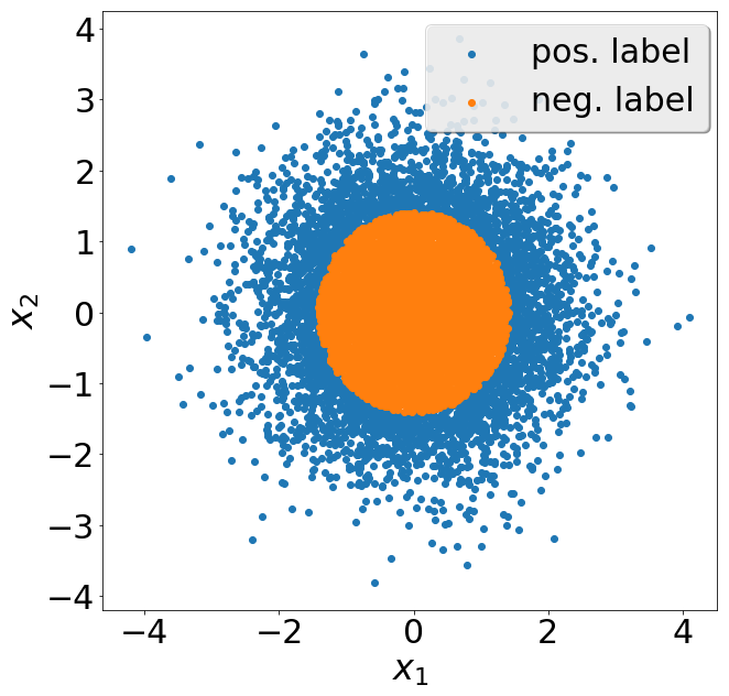
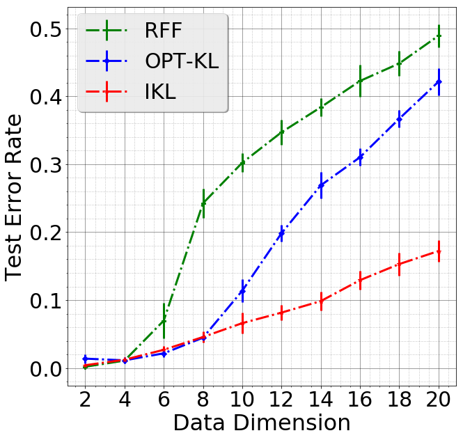
Figure 4: Left figure is training examples when $d=2$. Right figure is the classification error v.s. data dimension.

Kernel learning with a poor choice of $\mathbb{P}_{k}(\omega)$

We generate $\{x_{i}\}_{i=1}^{n}\sim\mathcal{N}(0,I_{d})$ with $y_{i}=\text{sign}(\|x\|_{2}-\sqrt{d})$, where $d$ is the data dimension. A two dimensional example is shown in Figure 4. Competitive baselines include random features (RFF) (Rahimi and Recht,, 2007) as well as OPT-KL (Sinha and Duchi,, 2016). In the experiments, we fix $M=256$ in RKS for all algorithms. Since Gaussian kernels with the bandwidth $\sigma=1$ is known to be ill-suited for this task (Sinha and Duchi,, 2016), we directly use random features from it for RFF and OPT-KL. Similarly, we set $\mathbb{P}(\nu)$ to be standard normal distribution as well.

The test error for different data dimension $d=\{2,4,\ldots,18,20\}$ is shown in Figure 4. Note that RFF is competitive with OPT-KL and IKL when $d$ is small ($d\leq 6$), while its performance degrades rapidly as $d$ increases, which is consistent with the observation in Sinha and Duchi, (2016). More discussion of the reason of failure can be referred to Sinha and Duchi, (2016). On the other hand, although using standard normal as the spectral distribution is ill-suited for this task, both OPT-KL and IKL can adapt with data and learn to transform it into effective kernels and result in slower degradation with $d$.

Note that OPT-KL learns the sparse weights on the sampled random features ($M=256$). However, the sampled random features can fail to contain informative ones, especially in high dimension (Bullins et al.,, 2018). Thus, when using limited amount of random features, OPT-IKL may result in worse performance than IKL in the high dimensional regime in Figure 4.

Performance on benchmark datasets

Next, we evaluate our IKL framework on standard benchmark binary classification tasks. Challenging label pairs are chosen from MNIST (LeCun et al.,, 1998) and CIFAR-10 (Krizhevsky and Hinton,, 2009) datasets; each task consists of $10000$ training and $2000$ test examples. For all datasets, raw pixels are used as the feature representation. We set the bandwidth of RBF kernel by the median heuristic. We also compare with Wilson and Adams, (2013), the spectral mixture (SM) kernel, which uses Gaussian mixture to learn spectral density and can be seen as the explicit generative model counterpart of IKL. Also, SM kernel is a MKL variant with linear combination (Gönen and Alpaydın,, 2011). In addition, we consider the joint training of random features and model parameters, which can be treated as two-layer neural network (NN) and serve as the lower bound of error for comparing different kernel learning algorithms.

The test error versus different $M=\{2^{6},2^{7},\ldots,2^{13}\}$ in the second stage are shown in Figure 5. First, in light of computation efficiency, SM and the proposed IKL only sample $m=64$ random features in each iteration in the first stage, and draws different number of basis $M$ from the learned $h_{\psi}(\nu)$ for the second stage. OPT-KL, on the contrary, the random features used in training and testing should be the same. Therefore, OPT-IKL needs to deal with $M$ random features in the training. It brings computation concern when $M$ is large. In addition, IKL demonstrates improvement over the representative kernel learning method OPT-KL, especially significant on the challenging datasets such as CIFAR-10. In some cases, IKL almost reaches the performance of NN, such as MNIST, while OPT-KL degrades to RFF except for small number of basis $(M=2^{6})$. This illustrates the effectiveness of learning kernel spectral distribution via the implicit generative model $h_{\psi}$. Also, IKL outperforms SM, which is consistent with the finding in Section 3 that IKL can learn more complicated spectral distributions than simple mixture models (SM).

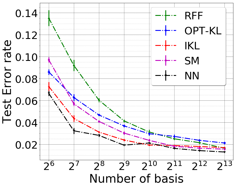
(a) MNIST (4-9)

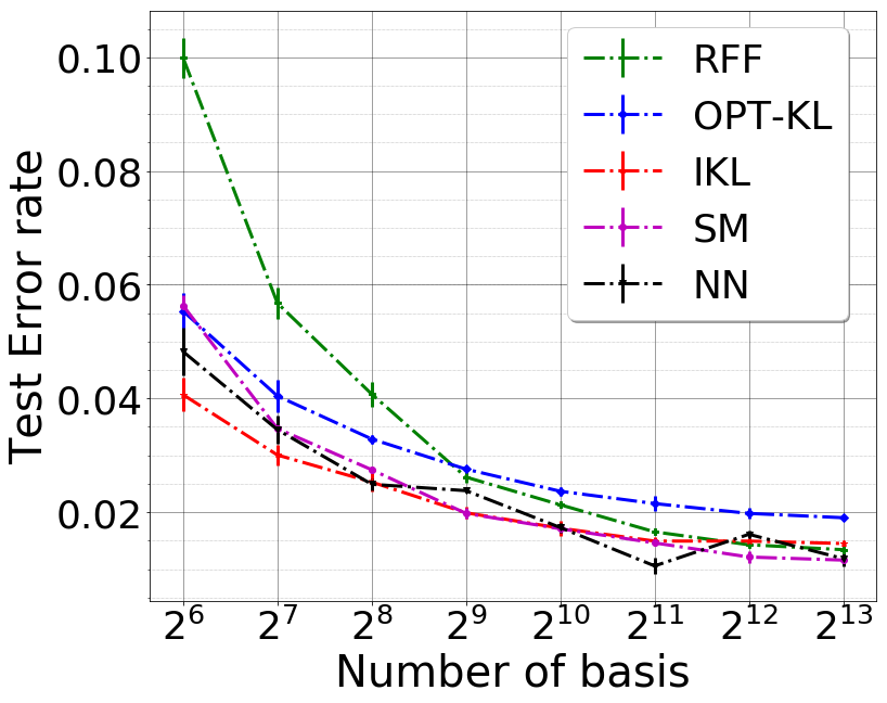
(b) MNIST (5-6)

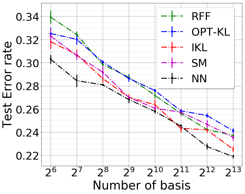
(c) CIFAR-10 (auto-truck)

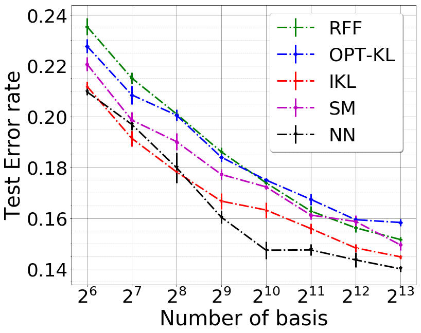
(d) CIFAR-10 (plane-bird)

Figure 5: Test error rate versus number of basis in second stage on benchmark binary classification tasks. We report mean and standard deviation over five runs. Our method (IKL) is compared with RFF (Rahimi and Recht,, 2009), OPT-KL (Sinha and Duchi,, 2016), SM (Wilson and Adams,, 2013) and the end-to-end training MLP (NN).

4.2 Consistency and Generalization

The simple two-stages approach, IKL with RKS, allows us to provide the consistency and generalization guarantees. For consistency, it guarantees the solution of finite sample approximations of  (9) approach to the optimum of  (9) (population optimum), when we increase number of training data and number of random features. We firstly define necessary symbols and state the theorem.

Let $s(x_{i},x_{j})=y_{i}y_{j}$ be a label similarity function, where $|y_{i}|\leq 1$. We use $s_{ij}$ to denote $s(x_{i},x_{j})$ interchangeably. Given a kernel $k$, we define the true and empirical alignment functions as,

$$\begin{array}[]{ccl}T(k)&=&\mathbb{E}\left[s(x,x^{\prime})k(x,x^{\prime})\right]\\ \hat{T}(k)&=&\frac{1}{n(n-1)}\sum_{i\neq j}s_{ij}k(x_{i},x_{j}).\\ \end{array}$$

In the following, we abuse the notation $k_{\psi}$ to be $k_{h}$ for ease of illustration. Recall the definitions of $k_{h}(x,x^{\prime})=\langle\phi_{h}(x),\phi_{h}(x^{\prime})\rangle$ and $\hat{k}_{h}(x,x^{\prime})=\hat{\phi}_{h}(x)^{\top}\hat{\phi}_{h}(x^{\prime})$. We define two hypothesis sets

$$\begin{array}[]{l}\displaystyle\mathcal{F}_{\mathcal{H}}=\{f(x)=\langle w,\phi_{h}(x)\rangle_{H}|h\in\mathcal{H},\langle w,w\rangle\leq 1\}\\ \displaystyle\hat{\mathcal{F}}_{\mathcal{H}}^{m}=\{f(x)=w^{\top}\hat{\phi}_{h}(x)|h\in\mathcal{H},\|w\|\leq 1,w\in\mathbb{R}^{m}\}.\end{array}$$

Definition 4.

(Rademacher’s Complexity) Given a hypothesis set $\mathcal{F}$, where $f:\mathcal{X}\times\mathcal{X}\rightarrow\mathbb{R}$ if $f\in\mathcal{F}$, and a fixed sample $X=\{x_{1},\dots,x_{n}\}$, the empirical Rademacher’s complexity of $\mathcal{F}$ is defined as

$$\mathfrak{R}_{X}^{n}(\mathcal{F})=\frac{1}{n}\mathbb{E}_{\sigma}\left[\sup_{f\in\mathcal{F}}\sum_{i=1}^{n}\sigma_{i}f(x_{i})\right],$$

where $\sigma$ are $n$ i.i.d. Rademacher random variables.

We then have the following theorems showing that the consistency guarantee depends on the complexity of the function class induced by IKL as well as the number of random features. The proof can be found in Appendix D.

Theorem 5.

(Consistency) Let $\hat{h}=\arg\max_{h\in\mathcal{H}}\hat{T}(\hat{k}_{h})$, with i.i.d, samples $\{\nu_{i}\}_{i=1}^{m}$ drawn from $\mathbb{P}(\nu)$. With probability at least $1-3\delta$, we have $|T(\hat{k}_{\hat{h}})-\sup_{h\in\mathcal{H}}T(k_{h})|\leq$

$$\begin{array}[]{c}\displaystyle 2\mathbb{E}_{X}\left[\mathfrak{R}_{X}^{n-1}(\mathcal{F}_{\mathcal{H}})+\mathfrak{R}_{X}^{n-1}(\hat{\mathcal{F}}_{\mathcal{H}}^{m})\right]+\sqrt{\frac{8\log\frac{1}{\delta}}{n}}+\sqrt{\frac{2\log\frac{4}{\delta}}{m}}.\end{array}$$

Applying Cortes et al., (2010), We also have a generalization bound, which depends number of training data $n$, number of random features $m$ and the Rademacher complexity of IKL kernel, as shown in Appendix E. The Rademacher complexity $\mathfrak{R}_{X}^{n}(\mathcal{F}_{\mathcal{H}})$, for example, can be $1/\sqrt{n}$ or even $1/n$ for kernels with different bounding conditions (Cortes et al.,, 2013). We would expect worse rates for more powerful kernels. It suggests the trade-off between consistency/generalization and using powerful kernels parametrized by neural networks.

5 Discussion

We propose a generic kernel learning algorithm, IKL, which learns sampling processes of kernel spectral distributions by transforming samples from a base distribution $\mathbb{P}(\nu)$ into ones for the other kernel (spectral density). We compare IKL with other algorithms for learning MMD GAN and supervised learning with Random Kitchen Sinks (RKS). For these two tasks, the conditions and guarantees of IKL for are studied. Empirical studies show IKL is better than or competitive with the state-of-the-art kernel learning algorithms. It proves IKL can learn to transform $\mathbb{P}(\nu)$ into effective kernels even if $\mathbb{P}(\nu)$ is less less favorable to the task.

We note that the preliminary idea of IKL is mentioned in Băzăvan et al., (2012), but they ended up with a algorithm that directly optimizes sampled random features (RF), which has many follow-up works (e.g. Sinha and Duchi, (2016); Bullins et al., (2018)). The major difference is, by learning the transformation function $h_{\psi}$, the RF used in training and evaluation can be different. This flexibility allows a simple training algorithm (SGD) and does not require to keep learned features. In our studies on GAN and RKS, we show using a simple MLP can already achieve better or competitive performance with those works, which suggest IKL can be a new direction for kernel learning and worth more studies.

We highlight that IKL is not conflict with existing works but can be combined with them. In Section 3, we show combining IKL with kernel learning via embedding (Wilson et al.,, 2016) and mixture of spectral distributions (Wilson and Adams,, 2013). Therefore, in addition to the examples shown in Section 3 and Section 4, IKL is directly applicable to many existing works with kernel learning via embedding (e.g. Dai et al., (2014); Li and Póczos, (2016); Wilson et al., (2016); Al-Shedivat et al., (2016); Arbel et al., (2018); Jean et al., (2018); Chang et al., (2019)). A possible extension is combining with Bayesian inference (Oliva et al.,, 2016) under the framework similar to Saatchi and Wilson, (2017). The learned sampler from IKL can possibly provide an easier way to do Bayesian inference via sampling.

Appendix A Proof of Theorem 2

We first show $\mathbb{P}_{n}\xrightarrow[]{D}\mathbb{P}$ then $\max_{\psi,\varphi}M_{\psi,\varphi}(\mathbb{P},\mathbb{P}_{n})\rightarrow 0$. The results are based on Arbel et al., (2018), which leverages Corollary 11.3.4 of Dudley, (2018). Follows the sketch of Arbel et al., (2018), the only thing we remain to show is proving $\|k_{\psi}(f_{\varphi}(x),\cdot)-k_{\psi}(f_{\varphi}(y),\cdot)\|_{\mathcal{H}_{K}}$ is Lipschitz. By definition, we know that $\|k_{\psi}(f_{\varphi}(x),\cdot)-k_{\psi}(f_{\varphi}(y),\cdot)\|_{\mathcal{H}_{K}}=2(1-k_{\psi}(f_{\varphi}(x),f_{\varphi}(y)))$. Also, since $k_{\psi}(0)=1$ and $k_{\psi}(0)-k_{\psi}(x,x^{\prime})\leq L_{k}\|0-(x-x^{\prime})\|$ (Lipschtiz assumption of $k_{\psi}$), we have

$$\|k_{\psi}(f_{\varphi}(x),\cdot)-k_{\psi}(f_{\varphi}(y),\cdot)\|_{\mathcal{H}_{K}}\leq 2L_{k}\|f_{\varphi}(x)-f_{\varphi}(y)\|\leq 2L_{k}L\|x-y\|,$$

where the last inequality is since $f_{\varphi}$ is also a Lipschitz function with Lipschitz constant $L$.

The other direction, $\max_{\psi,\varphi}M_{\psi,\varphi}(\mathbb{P},\mathbb{P}_{n})\rightarrow 0$ then $\mathbb{P}_{n}\xrightarrow[]{D}\mathbb{P}$, is relatively simple. Without loss of generality, we assume there exists $\psi^{\prime}$ and $\phi^{\prime}$ such that $h_{\psi}$ and $f_{\phi}$ are identity functions (up to scaling), which recover the Gaussian kernel $k$. Therefore, $\max_{\psi,\varphi}M_{\psi,\varphi}(\mathbb{P},\mathbb{P}_{n})\rightarrow 0$ implies $M_{\psi^{\prime},\varphi^{\prime}}(\mathbb{P},\mathbb{P}_{n})\rightarrow 0$, which completes the proof because MMD with any Gaussian kernel is weak (Gretton et al.,, 2012).

A.1 Continuity

Lemma 6.

(Borisenko and Minchenko, (1992)) Define $\tau(x)=\max\{f(x,u)|u\in U\}$. If $f$ is locally Lipschitz in $x$, $U$ is compact and $\bigtriangledown f(x,u^{*}(x))$ exists, where $u^{*}(x)=\arg\max_{u}f(x,u)$, then $\tau(x)$ is differentiable almost everywhere.

We are going to show

$$\max_{\psi,\varphi}M_{\psi,\varphi}(\mathbb{P}_{\mathcal{X}},\mathbb{P}_{\theta})=\mathbb{E}_{x,x^{\prime}}[k_{\psi,\varphi}(x,x^{\prime})]-2\mathbb{E}_{x,z}[k_{\psi,\varphi}(x,g_{\theta}(z))]+\mathbb{E}_{z,z^{\prime}}[k_{\psi,\varphi}(g_{\theta}(z^{\prime}),g_{\theta}(z))]$$ (10)

is differentiable with respect to $\varphi$ almost everywhere by using the auxiliary Lemma 6. We fist show $\mathbb{E}_{z,z^{\prime}}[k_{\psi,\varphi}(g_{\theta}(z^{\prime}),g_{\theta}(z))]$ in (10) is locally Lipschitz in $\theta$. By definition, $k_{\psi,\varphi}(x,x^{\prime})=k_{\psi}(f_{\varphi}(x)-f_{\varphi}(x^{\prime}))$, therefore,

$$\mathbb{E}_{x,x^{\prime}}\bigg{[}k_{\psi,\varphi}\Big{(}g_{\theta}(z),g_{\theta}(z^{\prime})\Big{)}-k_{\psi,\varphi}\Big{(}g_{\theta^{\prime}}(z),g_{\theta^{\prime}}(z^{\prime})\Big{)}\bigg{]}$$

$$= \mathbb{E}_{z,z^{\prime}}\bigg{[}k_{\psi}\Big{(}f_{\varphi}\big{(}g_{\theta}(z)\big{)}-f_{\varphi}\big{(}g_{\theta}(z^{\prime})\big{)}\Big{)}\bigg{]}-\mathbb{E}_{z,z^{\prime}}\bigg{[}k_{\psi}\Big{(}f_{\varphi}\big{(}g_{\theta^{\prime}}(z)\big{)}-f_{\varphi}\big{(}g_{\theta^{\prime}}(z^{\prime})\big{)}\Big{)}\bigg{]}$$

$$\leq \mathbb{E}_{z,z^{\prime}}\bigg{[}L_{k}\Big{\|}f_{\varphi}\big{(}g_{\theta}(z)\big{)}-f_{\varphi}\big{(}g_{\theta}(z^{\prime})\big{)}-f_{\varphi}\big{(}g_{\theta^{\prime}}(z)\big{)}+f_{\varphi}\big{(}g_{\theta^{\prime}}(z^{\prime})\big{)}\Big{\|}\bigg{]}$$

$$\leq \mathbb{E}_{z,z^{\prime}}\Big{[}L_{k}L(\theta,z)\|\theta-\theta^{\prime}\|+L_{k}L(\theta,z^{\prime})\|\theta-\theta^{\prime}\|\Big{]}$$

$$= 2L_{k}\mathbb{E}_{z}\big{[}L(\theta,z)\big{]}\|\theta-\theta^{\prime}\|.$$

The first inequality is followed by the assumption that $k$ is locally Lipschitz in $(x,x^{\prime})$, with a upper bound $L_{k}$ for Lipschitz constants. By Assumption 1, $\mathbb{E}_{z}\big{[}L(\theta,z)\big{]}<\infty$, we prove $\mathbb{E}_{z,z^{\prime}}\Big{[}k_{\psi}\big{(}f_{\varphi}(g_{\theta}(z))-f_{\varphi}(g_{\theta}(z^{\prime}))\big{)}\Big{]}$ is locally Lipschitz. The similar argument is applicable to other terms in (10); therefore, (10) is locally Lipschitz in $\theta$.

Last, with the compactness assumption on $\Phi$ and $\Psi$, and differentiable assumption on $M_{\psi,\varphi}(\mathbb{P}_{\mathcal{X}},\mathbb{P}_{\theta})$, applying Lemma 6 proves Theorem 2.

Appendix B Proof of Lemma 3

Without loss of the generality, we can rewrite the kernel function as $k_{\psi}(t)=\mathbb{E}_{\nu}\Big{[}\cos\big{(}h_{\psi}(\nu)^{\top}t\big{)}\Big{]}$, where $t$ is bounded. We then have

$$\begin{array}[]{ccl}\|\nabla_{t}k_{\psi}(t)\|&=&\Big{\|}\mathbb{E}_{\nu}\Big{[}\sin\big{(}h_{\psi}(\nu)^{\top}t\big{)}h_{\psi}(\nu)\Big{]}\Big{\|}\\ &\leq&\mathbb{E}_{\nu}\Big{[}\big{|}\sin(h_{\psi}(\nu)^{\top}t)\big{|}\times\|h_{\psi}(\nu)\|\Big{]}\\ &\leq&\mathbb{E}_{\nu}\big{[}\|t\|\|h_{\psi}(\nu)\|^{2}\big{]}\end{array}$$

The last inequality follows by $|\sin(x)|<|x|$. Since $t$ is bounded, if $\mathbb{E}_{\nu}[\|h_{\psi}(\nu)\|^{2}]<\infty$, there exist a constant $L$ such that $\|\nabla_{t}k_{\psi}(t)\|<L,\forall t$.

By mean value theorem, for any $t$ and $t^{\prime}$, there exists $s=\alpha t+(1-\alpha)t^{\prime}$, where $\alpha\in[0,1]$, such that

$$k_{\psi}(t)-k_{\psi}(t^{\prime})=\nabla_{s}k_{\psi}(s)^{\top}(t-t^{\prime}).$$

Combining with $\|\nabla_{t}k_{\psi}(t)\|<L,\forall t$, we prove

$$k_{\psi}(t)-k_{\psi}(t^{\prime})\leq L\|t-t^{\prime}\|.$$

Appendix C Additional Studies of MMD GAN with IKL

C.1 Additional Quantitative Results

We show the full quantitative results on MMD GANs with different kernels with mean and standard error in Table 2. In every tasks, IKL is the best among the predefined base kernels (Gaussian, RQ) and the competitive kernel learning algorithm (SM). The difference in FID is less significant than inception score and JS-4, but we note that FID score is a biased evaluation metric as discussed in Bińkowski et al., (2018).

Method	Inception Scores $(\uparrow)$	FID Scores $(\downarrow)$	JS-4 $(\downarrow)$
Gaussian	$6.726\pm 0.021$	$32.50\pm 0.07$	$0.381\pm 0.003$
RQ	$6.785\pm 0.031$	$32.20\pm 0.09$	$0.463\pm 0.005$
SM	$6.746\pm 0.031$	$32.43\pm 0.08$	$0.378\pm 0.003$
IKL	$\mathbf{6.876\pm 0.018}$	$\mathbf{31.98\pm 0.05}$	$\mathbf{0.372\pm 0.002}$
WGAN-GP	$6.539\pm 0.034$	$36.413\pm 0.05$	$0.379\pm 0.002$

Table 2: Inception scores, FID scores, and JS-4 divergece results.

C.2 Computational Issues of GAN trainings with IKL

Model Capacity

For $f_{\varphi}$, the number of parameters for DCGAN is around $0.8$ million for size $32\times 32$ images and $3$ millions for size $64\times 64$ images. The ResNet architecture used in Gulrajani et al., (2017) has around $10$ millions parameters. In contrast, in all experiments, we use simple three layer MLP as $h_{\psi}$ for IKL, where the input and output dimensions are 16, and hidden layer size is 32. The total parameters are just around 2,000. Compared with $f_{\phi}$, the additional number of parameters used for $h_{\psi}$ is almost negligible.

Computational Time

The potential concern of IKL is sampling random features for each examples. In our experiments, we use $m=1024$ random features for each iteration. We measure the time per iteration of updating critic iterations ($f$ for WGAN-GP and MMD GAN with Gaussian kernel; $f$ and $h$ for IKL) with different batch sizes under Titan X. The difference between WGAN-GP, MMD GAN and IKL are not significant. The reason is computing MMD and random feature is highly parallelizable, and other computation, such as evaluating $f_{\phi}$ and its gradient penalty, dominates the cost because $f_{\phi}$ has much more parameters as aforementioned. Therefore, we believe the proposed IKL is still cost effective in practice.

C.3 Detailed Discussion of Variance Constraints

In Section 3, we propose to constrain variance via $\lambda_{h}(\mathbb{E}_{\nu}\left[\|h_{\psi}(\nu)\|^{2}\right]-u)^{2}$. There are other alternatives, such as constraining $L^{2}$ penalty or using Langrange. In practice, we do not observe significant difference.

Although we show the necessity of the variance constraint in language generation in Figure 3, we remark that the proposed constraint is a sufficient condition. For CIFAR-10, without the constraint, we observe that the variance is still bouncing between $1$ and $2$ without explosion as Figure 3. Therefore, the training leads to a satisfactory result with $6.731\pm 0.034$ inception score, but it is slightly worse than IKL in Table 1. The necessary or weaker sufficient conditions are worth further studying as a future work.

C.4 IKL with and without Neural Networks on GAN training

Instead of learning a transform function $h_{\psi}$ for the spectral distribution as we proposed in Section 2 (IKL-NN), the other realization of IKL is to keep a pool of finite number learned random features $\Omega=\{\hat{\omega_{i}}\}_{i=1}^{m}$, and approximate the kernel evaluation by $\hat{k}_{\Omega}(x,x^{\prime})=\hat{\phi}_{\Omega}(x)^{\top}\hat{\phi}_{\Omega}(x^{\prime})$, where $\hat{\phi}_{\Omega}(x)^{\top}=[\phi(x;\hat{\omega}_{1}),\dots,\phi(x;\hat{\omega}_{m})]$. During the learning, it directly optimize $\hat{\omega_{i}}$. Many existing works study this idea for supervised learning, such as Băzăvan et al., (2012); Yang et al., (2015); Sinha and Duchi, (2016); Chang et al., (2017); Bullins et al., (2018). We call the latter realization as IKL-RFF. Next, we discuss and compare the difference between IKL-NN and IKL-RFF.

The crucial difference between IKL-NN and IKL-RFF is, IKL-NN can sample arbitrary number of random features by first sampling $\nu\sim\mathbb{P}(\nu)$ and transforming it via $h_{\psi}(\nu)$, while IKL-RFF is restricted by the pool size $m$. If the application needs more random features, IKL-RFF will be memory inefficient. Specifically, we compare IKL-NN and IKL-RFF with different number of random features in Figure 6. With the same number of parameters (i.e., $|h_{\psi}|=m\times dim(\nu)$) , IKL-NN outperforms IKL-RFF of $m=128$ on Inception scores ($6.876$ versus $6.801$). For IKL-RFF to achieve the same or better Inception scores of IKL-NN, the number of random features $m$ needs increasing to $4096$, which is less memory efficient than the IKL-NN realization. In particular, $h_{\psi}$ of IKL-NN is a three-layers MLP with $2048$ number of parameters ($16\times 32+32\times 32+32\times 16$), while IKL-RFF has $2048,65536$ number of parameters, for $m=128,4096$, respectively.

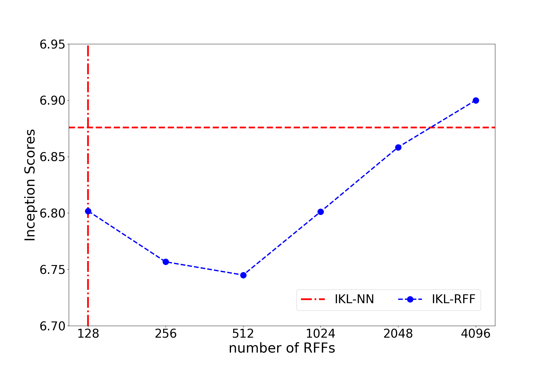
Figure 6: The comparison between IKL-NN and IKL-RFF on CIFAR-10 under different number of random features.

Algorithm	JS-4
IKL-NN	$0.372\pm 0.002$
IKL-RFF	$0.383\pm 0.002$
IKL-RFF (+2)	$0.380\pm 0.002$
IKL-RFF (+4)	$0.377\pm 0.002$
IKL-RFF (+8)	$0.375\pm 0.002$

Table 3: The comparison between IKL-NN and IKL-RFF on Google Billion Word.

On the other hand, using large $m$ for IKL-RFF not only increases the number of parameters, but might also enhance the optimization difficulty. Zhang et al., (2017) discuss the difficulty of optimizing RFF directly on different tasks. Here we compare IKL-NN and IKL-RFF on challenging Google Billion Word dataset. We train IKL-RFF with the same setting as Section 3.3 and Appendix F.1, where we set the pool size $m$ to be $1024$ and the updating schedule between critic and generator to be $10:1$, but we tune the Adam optimization parameter for IKL-RFF for fair comparison. As discussed above, please note that the number of parameters for $h_{\psi}$ is $2048$ while IKL-RFF uses $16384$ when $m=1024$. The results are shown in Table 3. Even IKL-RFF is using more parameters, the performance $0.383$ is not competitive as IKL-NN, which achieves $0.372$.

In Algorithm 1, we update $f_{\varphi}$ and $h$ in each iteration with $n_{c}$ times, where we use $n_{c}=10$ here. We keep the number of updating $f_{\varphi}$ to be $10$, but increase the number of update for $\{\hat{\omega_{i}}\}_{i=1}^{1}024$ to be $12,14,18$ in each iteration. The result is shown in Table 3 with symbols +2, +4 and +8 respectively. Clearly, we see IKL-RFF need more number of updates to achieve competitive performance with IKL-NN. The results might implies IKL-RFF is a more difficult optimization problem with more parameters than IKL-NN. It also confirms the effectiveness of learning implicit generative models with deep neural networks Goodfellow et al., (2014), but the underlying theory is still an open research question. A better optimization algorithm Zhang et al., (2017) may improve the performance gap between IKL-NN and IKL-RFF, which worth more study as future work.

Appendix D Proof of Theorem 5

We first prove two Lemmas.

Lemma 7.

(Consistency with respect to data) With probability at least $1-\delta$, we have

$$\sup_{h\in\mathcal{H}}|\hat{T}(k_{h})-T(k_{h})|\leq 2\mathbb{E}_{X}\bigg{[}\mathfrak{R}_{X}^{n-1}(\mathcal{F}_{\mathcal{H}})\bigg{]}+\sqrt{\frac{2}{n}\log{\frac{1}{\delta}}}$$

Proof.

Define

$$\rho(x_{1},\dots,x_{n})=\sup_{h\in\mathcal{H}}|\hat{T}(k_{h})-T(k_{h})|,$$

since $|k_{h}(x,x^{\prime})|\leq 1$, it is clearly

$$\begin{array}[]{cl}\displaystyle\sup_{x_{1},\dots,x_{i},x_{i}^{\prime},\dots,x_{n}}&|\rho(x_{1},\dots,x_{i},\dots x_{n})-\\ &\rho(x_{1},\dots,x_{i}^{\prime},\dots x_{n})|\leq\frac{2}{n}.\end{array}$$

Applying McDiarmids Inequality, we get

$$\mathbb{P}\left(\rho(x_{1},\dots,x_{n})-\mathbb{E}[\rho(x_{1},\dots,x_{n})]\geq\epsilon\right)\leq\exp\left(\frac{-n\epsilon^{2}}{2}\right).$$

By Lemma 8, we can bound

$$\mathbb{E}[\rho(x_{1},\dots,x_{n})]\leq 2\mathbb{E}_{X}\bigg{[}\mathfrak{R}_{X}^{n-1}(\mathcal{F}_{\mathcal{H}})\bigg{]}$$

and finish the proof. ∎

Lemma 8.

Given $X=\{x_{1},\dots,x_{n}\}$, define

$$\rho(x_{1},\dots,x_{n})=\sup_{h\in\mathcal{H}}|\hat{T}(k_{h})-T(k_{h})|,$$

we have

$$\mathbb{E}\bigg{[}\rho(x_{1},\dots,x_{n})\bigg{]}\leq 2\mathbb{E}_{X}\bigg{[}\mathfrak{R}_{X}^{n-1}(\mathcal{F}_{\mathcal{H}})\bigg{]},$$

Proof.

The proof is closely followed by Dziugaite et al., (2015). Given $h$, we first define $t_{h}(x,x^{\prime})=s(x,x^{\prime})k_{h}(x,x^{\prime})$ as a new kernel function to simplify the notations. We are then able to write

$$\begin{array}[]{cl}&\mathbb{E}\bigg{[}\rho(x_{1},\dots,x_{n})\bigg{]}\\ =&\displaystyle\mathbb{E}_{X}\bigg{[}\sup_{h_{\in}\mathcal{H}}\left|\mathbb{E}\bigg{[}t_{h}(z,z^{\prime})\bigg{]}-\frac{1}{n(n-1)}\sum_{i\neq j}t_{h}(x_{i},x_{j})\right|\bigg{]}\\ \leq&\displaystyle\mathbb{E}_{X,Z}\bigg{[}\sup_{h_{\in}\mathcal{H}}\left|\frac{1}{n(n-1)}\sum_{i\neq j}\left(t_{h}(z_{i},z_{j})-t_{h}(x_{i},x_{j})\right)\right|\bigg{]}\end{array}$$

by using Jensen’s inequality. Utilizing the conditional expectation and introducing the Rademacher random variables $\{\sigma_{i}\}_{i=1}^{n-1}$, we can write the above bound to be

$$\displaystyle\frac{1}{n}\sum_{i}\mathbb{E}_{X_{-i},Z_{-i}}\mathbb{E}_{x_{i},z_{i}}\bigg{[}\sup_{h_{\in}\mathcal{H}}\left|\frac{\sum_{i\neq j}t_{h}(z_{i},z_{j})-t_{h}(x_{i},x_{j})}{n-1}\right|\bigg{]}$$

$$=\displaystyle\mathbb{E}_{X,Z}\mathbb{E}_{X^{\prime},Z^{\prime},\sigma}\bigg{[}\sup_{h\in\mathcal{H}}\left|\frac{1}{n-1}\sum_{i=1}^{n-1}\sigma_{i}(t_{h}(z^{\prime},z_{n})-t_{h}(x^{\prime},x_{n}))\right|\bigg{]}$$ (11)

The equality follows by $X-X^{\prime}$ and $-(X-X^{\prime})$ has the same distributions if $X$ and $X^{\prime}$ are independent samples from the same distribution. Last, we can bound it by

$$\begin{array}[]{cl}\leq&\displaystyle\mathbb{E}_{X}\mathbb{E}_{\sigma,X^{\prime}}\bigg{[}\sup_{h\in\mathcal{H}}\left|\frac{2}{n-1}\sum_{i=1}^{n-1}\sigma_{i}t_{h}(x^{\prime},x_{i})\right|\bigg{]}\\ \leq&\displaystyle\mathbb{E}_{X}\mathbb{E}_{\sigma}\bigg{[}\sup_{f\in\mathcal{F}_{k_{\mathcal{H}}}}\left|\frac{2}{n-1}\sum_{i=1}^{n-1}\sigma_{i}f(x_{i})\right|\bigg{]}\\ =&2\mathbb{E}_{X}[\mathfrak{R}_{X}^{n-1}(\mathcal{F}_{\mathcal{H}})]\end{array}$$

The second inequality follows by $s(x,x^{\prime})\phi(x^{\prime})\in\mathcal{F}$ since $|s(x,x^{\prime})|\leq 1$.

∎

Lemma 9.

(Consistency with respect to sampling random features) With probability $1-\delta$, we have

$$|\sup_{h\in\mathcal{H}}\hat{T}(k_{h})-\sup_{h\in\mathcal{H}}\hat{T}(\hat{k}_{h})|\leq\sqrt{\frac{2\log\frac{4}{\delta}}{m}}$$

Proof.

Let the optimal solutions be

$$\begin{array}[]{ccl}h^{*}&=&\arg\max_{h\in\mathcal{H}}\hat{T}(k_{h})\\ \hat{h}&=&\arg\max_{h\in\mathcal{H}}\hat{T}(\hat{k}_{h}),\end{array}$$

By definition,

$$\begin{array}[]{cl}&\hat{T}(\hat{k}_{h})\\ =&\displaystyle\frac{1}{n(n-1)}\sum_{i\neq j}s_{ij}\left(\frac{1}{m}\sum_{k=1}^{m}\cos(h(\nu_{k})^{\top}(x_{i}-x_{j}))\right)\\ =&\displaystyle\frac{1}{m}\sum_{k=1}^{m}\left(\frac{1}{n(n-1)}s_{ij}\cos(h(\nu_{k})^{\top}(x_{i}-x_{j}))\right)\end{array}$$

It is true that $|\frac{1}{n(n-1)}s_{ij}\cos(h(\nu_{k})^{\top}(x_{i}-x_{j})|\leq 1$ since $|s_{ij}|<1$ and $|\cos(x)|<1$. we then have

$$\begin{array}[]{cl}&\mathbb{P}(|\sup_{h\in\mathcal{H}}\hat{T}(k_{h})-\sup_{h\in\mathcal{H}}\hat{T}(\hat{k}_{h})|>\epsilon)\\ \leq&\mathbb{P}(|\hat{T}(k_{h^{*}})-\hat{T}(\hat{k}_{h^{*}})|>\epsilon)+\mathbb{P}(|\hat{T}(k_{\hat{h}})-\hat{T}(\hat{k}_{\hat{h}})|>\epsilon)\\ \leq&\displaystyle 4\exp\left(-\frac{m\epsilon^{2}}{2}\right),\end{array}$$

where the last inequality follows from the Hoeffding’s inequality. ∎

With Lemma 7 and Lemma 9, we are ready to prove Theorem 5. We can decompose

$$\begin{array}[]{cl}&\displaystyle|T(\hat{k}_{\hat{h}})-\sup_{h\in\mathcal{H}}T(k_{h})|\\ \leq&\displaystyle|\sup_{h\in\mathcal{H}}T(k_{h})-\sup_{h\in\mathcal{H}}\hat{T}(k_{h})|+|\sup_{h\in\mathcal{H}}\hat{T}(k_{h})-\hat{T}(\hat{k}_{\hat{h}})|+|\hat{T}(\hat{k}_{\hat{h}})-T(\hat{k}_{\hat{h}})|\\ \leq&\displaystyle\sup_{h\in\mathcal{H}}|T(k_{h})-\hat{T}(k_{h})|+|\sup_{h\in\mathcal{H}}\hat{T}(k_{h})-\hat{T}(\hat{k}_{\hat{h}})|+\sup_{h\in\mathcal{H}}|\hat{T}(\hat{k}_{h})-T(\hat{k}_{h})|\end{array}$$

We then bound the first and third terms by Lemma 7 and the second term by Lemma 9. Last, using a union bound completes the proof.

Appendix E Generalization of Random Kitchen Sinks with IKL

Theorem 10.

(Generalization (Cortes et al.,, 2010)) Define the true and empirical misclassification for a classifier $f$ as $R(f)=\mathbb{P}(Yf(X)<0)$ and $\hat{R}_{\gamma}(h)=\frac{1}{n}\sum_{i=1}^{n}\min\left\{1,[1-yf(x_{i})/\gamma]_{+}\right\}$. Then

$$\sup_{f\in\hat{\mathcal{F}}_{\mathcal{H}}}\{R(f)-\hat{R}_{\gamma}(f)\}\leq\frac{2}{\gamma}\mathfrak{R}_{X}^{n}(\hat{\mathcal{F}}_{\mathcal{H}})+3\sqrt{\frac{\log\frac{2}{\delta}}{2n}}$$

with probability at least $1-\delta$.

Appendix F Hyperparameters

We report the hyperparameters used in the experiments.

F.1 GAN

For Gaussian kernels, we use $\sigma_{q}=\{1,2,4,8,16\}$ for images and $\sigma_{q}=\{0.5,1,2,4,8\}$ for text; for RQ kernels, we use $\alpha_{q}=\{0.2,0.5,1,2,5\}$ for images and $\alpha_{q}=\{0.04,0.1,0.2,0.4,1\}$ for text. We used Adam as optimizer. The learning rate for training both $f_{\phi}$ and $g_{\theta}$ is $0.0005$ and $0.0001$ for image and text experiments, respectively. The batch size $B$ is $64$. We set hyperparameter $n_{c}$ for updating critic to be $n_{c}=5$ and $n_{c}=10$ for CIFAR10 and Google Billion Word datasets. The learning rate of of $h_{\psi}$ for Adam is $10^{-6}$.

F.2 Random Kitchen Sinks with IKL

For OPT-KL, we use the code provided by Sinha and Duchi, (2016). We tune the hyperparameter $\rho=\{1.25,1.5,2,4,16,64\}$ on the validation set. For RFF, OPT-KL, and IKL, the linear classifier is Logistic Regression Fan et al., (2008), as to make reasonable comparison with MLP. We use $3$-fold cross validation to select the best $C$ on training set and present the error rate on test set. For CIFAR-10 and MNIST, we normalize data to be zero mean and one standard deviation in each feature dimension. The learning rate for Adam is $10^{-6}$. We follow Bullins et al., (2018) to use early stopping when performance on validation set does not gain.

References

- Al-Shedivat et al., (2016) Al-Shedivat, M., Wilson, A. G., Saatchi, Y., Hu, Z., and Xing, E. P. (2016). Learning scalable deep kernels with recurrent structure. arXiv preprint arXiv:1610.08936.
- Alber et al., (2017) Alber, M., Kindermans, P.-J., Schütt, K., Müller, K.-R., and Sha, F. (2017). An empirical study on the properties of random bases for kernel methods. In NIPS.
- Arbel et al., (2018) Arbel, M., Sutherland, D. J., Bińkowski, M., and Gretton, A. (2018). On gradient regularizers for mmd gans. In NIPS.
- Arjovsky and Bottou, (2017) Arjovsky, M. and Bottou, L. (2017). Towards principled methods for training generative adversarial networks. In ICLR.
- Arjovsky et al., (2017) Arjovsky, M., Chintala, S., and Bottou, L. (2017). Wasserstein GAN. In ICML.
- Bach, (2009) Bach, F. R. (2009). Exploring large feature spaces with hierarchical multiple kernel learning. In NIPS.
- Bach et al., (2004) Bach, F. R., Lanckriet, G. R., and Jordan, M. I. (2004). Multiple kernel learning, conic duality, and the smo algorithm. In ICML.
- Băzăvan et al., (2012) Băzăvan, E. G., Li, F., and Sminchisescu, C. (2012). Fourier kernel learning. In ECCV.
- Bellemare et al., (2017) Bellemare, M. G., Danihelka, I., Dabney, W., Mohamed, S., Lakshminarayanan, B., Hoyer, S., and Munos, R. (2017). The cramer distance as a solution to biased wasserstein gradients. arXiv preprint arXiv:1705.10743.
- Bińkowski et al., (2018) Bińkowski, M., Sutherland, D. J., Arbel, M., and Gretton, A. (2018). Demystifying mmd gans. In ICLR.