Reliable Deep Grade Prediction with Uncertainty Estimation

Abstract.

Currently, college-going students are taking longer to graduate than their parental generations. Further, in the United States, the six-year graduation rate has been 59% for decades. Improving the educational quality by training better-prepared students who can successfully graduate in a timely manner is critical. Accurately predicting students’ grades in future courses has attracted much attention as it can help identify at-risk students early so that personalized feedback can be provided to them on time by advisors. Prior research on students’ grade prediction include shallow linear models; however, students’ learning is a highly complex process that involves the accumulation of knowledge across a sequence of courses that can not be sufficiently modeled by these linear models. In addition to that, prior approaches focus on prediction accuracy without considering prediction uncertainty, which is essential for advising and decision making. In this work, we present two types of Bayesian deep learning models for grade prediction under a course-specific framework: i)Multilayer Perceptron (MLP) and ii) Recurrent Neural Network (RNN). These course-specific models are based on the assumption that prior courses can provide students with knowledge for future courses so that grades of prior courses can be used to predict grades in a future course. The MLP ignores the temporal dynamics of students’ knowledge evolution. Hence, we propose RNN for students’ performance prediction. To evaluate the performance of the proposed models, we performed extensive experiments on data collected from a large public university. The experimental results show that the proposed models achieve better performance than prior state-of-the-art approaches. Besides more accurate results, Bayesian deep learning models estimate uncertainty associated with the predictions. We explore how uncertainty estimation can be applied towards developing a reliable educational early warning system. In addition to uncertainty, we also develop an approach to explain the prediction results, which is useful for advisors to provide personalized feedback to students.

1. Introduction

The average six-year graduation rate for undergraduate programs in the United States has been around 59% for over a decade (Stillwell and Sable, 2013). More than half of the graduating students take six years to finish four-year programs. The additional time required by students and low graduation rates has high human, monetary and societal costs with regards to workforce training and economic growth. Lack of proper academic preparation and planning are some of the main reasons that lead to student failure in higher education (Anschuetz, 2015). To improve retention rates and help students graduate in a timely manner, we aim to develop analytics-driven early warning and degree planning systems that can identify at-risk students; so that advisors can provide them timely and personalized feedback/advice. Grade prediction is fundamental for these systems.

Prior next-term grade prediction methods usually train a one-size-fits-all model that predicts students’ grades in multiple courses (Polyzou and Karypis, 2016a). However, different courses have different characteristics such as prerequisites, knowledge content, instructors and difficulty level. To address this problem, Polyzou et al. proposed a course-specific framework, which was shown to be successful for accurately predicting students’ grades (Polyzou and Karypis, 2016a, b). Course-specific methods identify a subsets of prior courses on a course-by-course basis to predict a student’s grade in a target course. They are based on the assumption that students accumulate necessary knowledge to take future courses by taking a sequence of prior courses. Our models are based upon this course-specific framework.

From the perspective of educational psychology, learning is affected by both external and internal factors such as motivation, study habits, attention and instructor pedagogy (Mangal, 2002; Benjamin, 2014), which bring about challenges for grade prediction. These challenges are further exacerbated by the fact that learning is a reflection of human cognition which is a complex process (Piech et al., 2015). Existing course-specific models are linear shallow learners, e.g. linear regression or low-rank matrix factorization. These shallow learners may not be capable of capturing complex interactions underlying student’s learning. To better model students’ learning process, we propose to use deep learning models. Another drawback of traditional grade prediction methods is that the predicted grade is a point estimation. To make informed decision based on the predicted results, we need to know if the prediction system is confident or not. If the system is confident enough about the predictions, we can rely on them and take corresponding actions. However, if the prediction is not reliable, human advisors should decide what to do. Compared to traditional deep learning models, Bayesian deep learning models can provide principled uncertainty estimation.

Specifically, we propose two types of Bayesian deep learning models, (I) Multilayer Perceptron (MLP) (Rosenblatt, 1961), (II) Long Short Term Memory (LSTM) networks (Hochreiter and Schmidhuber, 1997). MLP consists of hierarchical hidden layers that maps the input vector to an output target. The input vector is treated as static and hence the temporal dynamics of the input data are ignored by MLP. To capture student’s knowledge evolution, we also propose a LSTM model. Theoretically, RNNs are able to model arbitrarily long sequential data. However, in practice, because of the vanishing gradient problem, vanilla RNNs fail to capture long-term dependencies. For grade prediction, a course taken several semesters ago might still have influence on the student’s performance in a future course. To model such long-term dependencies, we choose to use LSTM model.

The proposed models are evaluated on datasets extracted from University X by using different evaluation metrics. The results show that the proposed models outperform the comparative state-of-the-art methods in all aspects. To trust the predictions from a model, we need to know if the system is confident about its predictions or not. We provide empirical results about model uncertainty and investigate case studies towards developing a reliable educational early warning system. We also propose a method to explain the models’ predictions, which identifies a list of influential prior courses that lead to a student’s failure in the target course.

The main contributions of this work can be summarized as follows:

• We propose two types of course-specific Bayesian deep learning models for grade prediction, namely, course-specific MLP and LSTM. Compared to existing methods, the proposed models have better modeling capability and prediction accuracy.

• The proposed models can provide prediction uncertainty which is essential for decision making. Based on uncertainty estimation, we show how uncertainty can help build a reliable educational early warning system.

• In addition to uncertainty estimation, we propose a method to explain the prediction results, which can identify influential courses that results in a student’s failure of a course.

• We propose a method to evaluate the models’ capability of catching at-risk students. The evaluation results show that the proposed methods outperform several baseline methods for this task.

2. Related Work

The application of analytics to improve educational quality can be seen in many areas related to modeling of learners (Lan et al., 2014), predicting and advising learners (Elbadrawy et al., 2016), automated content enhancement (Agrawal et al., 2014), knowledge tracing (Yudelson et al., 2013; Corbett and Anderson, 1994) and course/topic recommendations to students (Elbadrawy and Karypis, 2016). Among them, student’s academic performance prediction has attracted much attention, as it underlies applications to several AI-based decision making systems including educational early warning systems, degree planning and academic trajectory planning (Elbadrawy et al., 2016). In light of this paper’s scope, we only review approaches for student’s performance prediction and predictive uncertainty estimation.

2.1. Student Performance Prediction

Several machine learning algorithms have been applied to tackle the student performance prediction problem (Bydžovská, 2015b; Sorour et al., 2015). Al-Barak et al. applied decision trees for grade prediction by using students’ transcript data (Al-Barrak and Al-Razgan, 2016). Umair et al. used Support Vector Machines (SVMs) to select key training instances for grade prediction (Umair and Sharif, 2018). Recommender systems based methods including collaborative filtering (Bydžovská, 2015a), matrix factorization (Koren et al., 2009) and factorization machines (Sweeney et al., 2016) have been proposed for grade prediction. These approaches use a one-size-fits-all framework for training the model and prediction. Polyzou et al. proposed a personalized model that is specific to each course and student (Polyzou and Karypis, 2016b). Student-course enrollment patterns have grouping structures which result in missing not at random patterns of student grade data. Leveraging this, Elbadrawy et al. proposed a domain-aware grade prediction algorithm for student’s performance prediction and course recommendation (Elbadrawy and Karypis, 2016). Since students accumulate knowledge by taking courses sequentially within the academic programs, it is assumed that the knowledge state of the students is evolving. Ren et al. proposed a temporal course-wise influence model which incorporates the influence of prior courses in a sequential way, however, up to two terms (Ren et al., 2017).

Several works use deep learning to model student learning habits and predict performance. Livieris et al. developed a neural network based classifier to predict whether a student will have poor performance in a Math course (Livieris et al., 2012). Gedeon et al. trained a feedforward neural network to predict a student’s final grade in a computer science course using data from teaching sessions and provided interpretability of the prediction results by generating a set of rules (Gedeon and Turner, 1993). Yang et al. designed a time series neural network using a student’s clickstream data while watching video lectures in massive open online courses (MOOCs) (Yang et al., 2017). Okubo et al. proposed a recurrent neural network classifier to predict a student’s grade by using data from various logs of learning activities (OKUBO et al., [n. d.]). For modeling student’s learning process within Intelligent Tutoring Systems (ITS), Piech et al. proposed using deep knowledge tracing (Piech et al., 2015). Most of the proposed neural network models were developed for in-class prediction or for intelligent tutoring systems that model student learning in a single course. The DKT models are similar to our proposed LSTM model; however, the DKT models only incorporate one response each time step. Our proposed LSTM model is more flexible and can incorporate several (responses) grades of prior courses taken together in the same semester.

The existing deep learning models either ignore the temporal dynamics of student’s grade data or are designed only for a single course by using data within that single course. In this paper, our proposed models aim to predict student’s performance by using data across several teaching sessions and the LSTM model can take into account the sequential aspect of a student accumulating knowledge across multiple semesters.

2.2. Predictive Uncertainty

Deep learning models have achieved state-of-the-art performance in many areas due to their abilities to model complex patterns (LeCun et al., 2015). However, general deep learning models cannot represent uncertainty, which is critical for decision-making. Bayesian models have the advantage of providing principled uncertainty estimation. Therefore, combining Bayesian approaches with deep learning models is a way to obtain benefits from these two perspectives. Figure 1 shows the difference between a traditional deep learning (neural network) and Bayesian deep learning model.

Bayesian deep learning models place a prior distribution over model parameters; the model is updated by Bayes’ rule with observed data. The posterior distribution of the model parameters is the learned model. Due to possible non-linear activation functions that can be applied to neurons, exact model posterior is not available. Approximate inference methods are used for model training, such as variational inference (Gal and Ghahramani, 2015). However, these methods have a high computational cost and are hard to scale in practice.

Recently, Monte Carlo (MC) dropout has been proposed by Gal et al. (Gal and Ghahramani, 2016), which is efficient for uncertainty estimation and requires no change in the designed model architecture. In this work, we adopt MC dropout as a way to estimate prediction uncertainty and explain the details in Section 3.4.

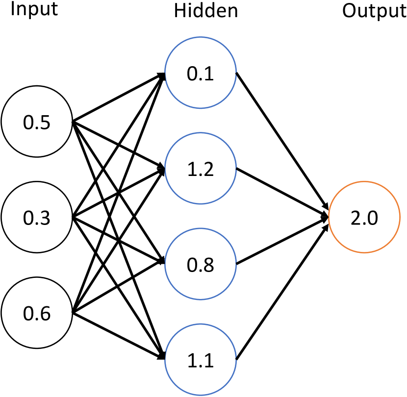
(a) Neural Netowrk

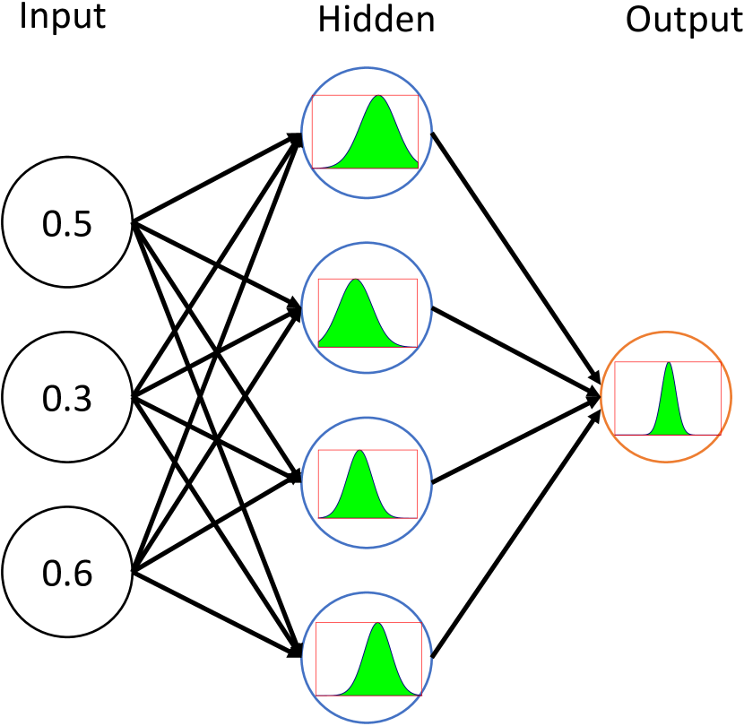
(b) Bayesian Neural Network

Figure 1. Comparision of Neural Network and Bayesian Neural Network

3. Methods

3.1. Model Learning Framework

Given records of $n$ students and $m$ courses, we extract the grades to form a sparse grade matrix $\mathbf{G}\in\mathbf{R}^{n\times m}$. In addition, we have the information associated with the semester (time) when the particular grade was obtained. Further, the data includes student-related features (e.g., academic level, previous GPAs, major, etc.) and course-related features (e.g., course level, discipline, credit hours, etc.). These content features are combined to form a feature vector associated with a student-course pair.

Given a student’s grades in the courses taken before the target course (referred to as prior courses), the objective of the next-term grade prediction problem is to predict the grade that the student will achieve in a course to be taken in the next semester (term). To predict grade in a course-wise manner, we adopt course-specific framework (Polyzou and Karypis, 2016b). Under this framework, different models are learnt for different courses. To predict a student’s grades in next courses, his/her grades from prior courses are fed into corresponding models.

3.2. Multilayer Perceptron

Traditional grade prediction models are linear models, such as linear regression. Compared to linear models, the key advantage of multilayer perceptron comes from its hierarchical hidden layers that capture complex interactions and non-linearities. The theoretical foundation is given by the Kolmogorov-Arnold representation theorem (Arnold, 1957; Kolmogorov, 1963); every multivariate continuous function can be represented as a superposition of one-dimensional continuous functions.

Given an input vector $\bm{x}$, the task of the multilayer perceptron algorithm is to map $\bm{x}$ to output $\bm{y}$, which has the following form

(1) $$\bm{y}=F(\bm{x})$$

To estimate a student’s grade in course $c$ by using the course-specifc MLP model $F^{c}$, we have

(2) $$\hat{y}^{c}=F^{c}(\mathbf{s})$$

where $\mathbf{s}\in\mathbb{R}^{m}$ is the vector of the student’s grades in the prior courses.

3.3. Long Short Term Memory

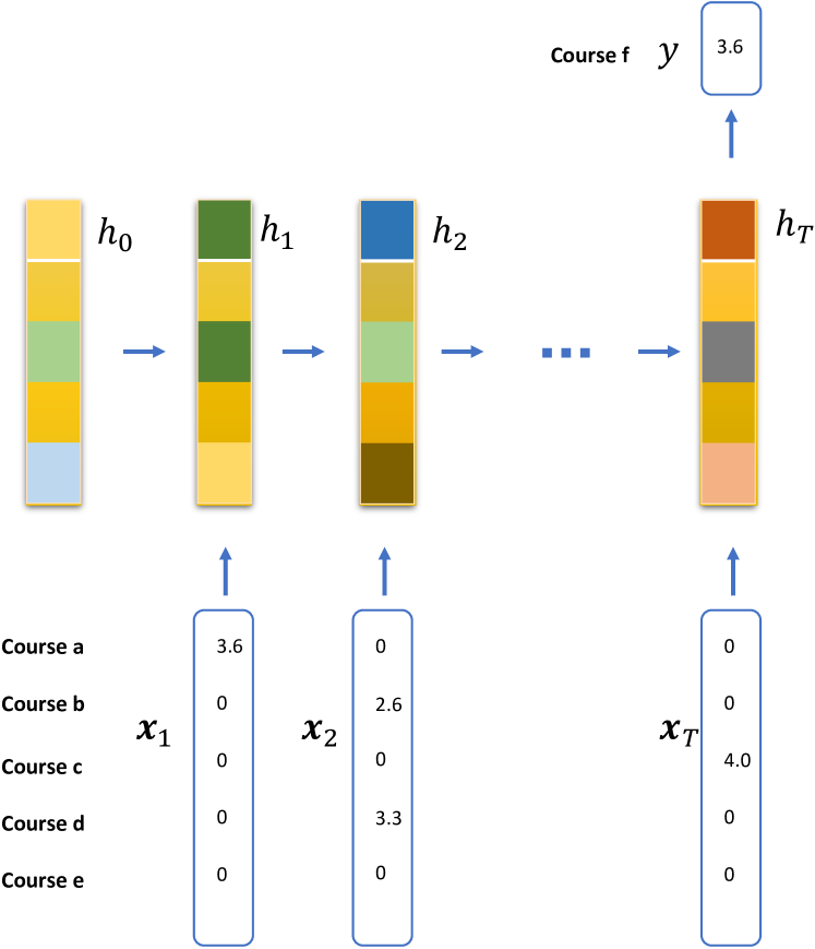
Figure 2. In this example, we want to predict a student’s grade in target course $f$ by using grades of the courses taken prior to course $f$ include $a,b,c,d,e$. $\bf{x}_{t}$ represents the grades of courses in term $t$. $y$ represents the predicted grade. The student took courses ($a$), ($b$, $d$), …, ($c$) in semester 1, 2, …, $T$ and obtained (3.6), (2.6, 3.3), …, (4.0) in this example, respectively.

To capture the sequential characteristics of students’ grades in prior courses, we model the learning behavior and performance using recurrent neural networks with long short term memory (Hochreiter and Schmidhuber, 1997) (LSTM). The standard RNN model has the vanishing gradient problem and is unable to capture long-range dependencies. In our case, an course taken several semesters before, such as a prerequisite, plays an important role in determining a student’s performance in a target course. To solve the long-term dependency problem, LSTM is proposed for sequential data. The hidden states of LSTM capture the student’s knowledge states, which models a student’s knowledge evolution. The hidden states are updated as the student enrolls for courses and obtain grades in them. Figure 2 shows the LSTM approach for modeling student’s learning process. At the beginning, a student has some prior knowledge before taking any courses; the student’s knowledge states evolve as he/she take courses, as indicated by different colors at each time step in Figure 2. A student’s knowledge states influences his/her performance in a course .The last hidden state $\mathbf{h}_{T}$ is used to predict his/her grade in a target course within the course-specific framework.

LSTM is a gated recurrent neural network, which consists of forget gate and input gate. The forget gate decides which part of the information to forget from the cell state. This is useful when the same knowledge can be obtained by taking two different courses. A student’s knowledge state corresponding to knowledge acquired by taking the first course can be discarded while renewed by using the second one. When student takes a new course, his/her knowledge state is updated. In LSTM, this is done by the information layer and input gate; input gate decides which new information should be added into the cell state. The output from LSTM is hidden state which represent student’s current knowledge state.

To estimate a student’s grade in the target course by using LSTM model, we first extract the student’s grades in the prior courses with timestamp i.e., in which terms the prior courses are taken. The grades in term $t$ are represented as multiple-hot encoded vector $\mathbf{x}_{t}$ — as more than one course can be taken together in one semester — where the entries of $\mathbf{x}_{t}$ corresponds to the grades of courses taken in semester $t$; $0$ represents the corresponding courses are not taken. If the grade obtained is 0 (F), we use a small number (0.1) to represent it to differentiate it from courses that are not taken. We input the sequence of the encoded vectors $\mathbf{x}_{1},\mathbf{x}_{2},...,\mathbf{x}_{T}$ to the model and the hidden state from the last step $\mathbf{h}_{T}$ is fed into a fully connected layer, the output of which is the predicted grade:

(3) $$y=\mathbf{w}_{yh}\cdot\mathbf{h}_{T}+b_{y}$$

where $\mathbf{h}_{T}$ is the last hidden state, $\mathbf{w}_{yh}$ is the parameters of the fully connected layer and $b_{y}$ is the bias term.

Table 1. Dataset Statistics

Major	Fall 2016			Spring 2017
	#S	#C	#G	#S	#C	#G
CS	2,664	18	22,246	3,728	19	33,039
ECE	1,160	16	16,415	1,421	15	23,459
BIOL	2,736	19	20,984	6,002	20	42,895
PSYC	2,980	20	14,966	4,628	20	23,560
CEIE	1,525	18	23,954	1,873	17	28,198
Overall	11065	91	98,565	17652	91	151,151

• #S number of students, #C number of courses, #G number of grades

3.4. Uncertainty Estimation

Given input data $\mathbf{x}$, the output of an Bayesian deep learning model $f(\cdot)$ is mean $\hat{y}$ and standard deviation $\sigma$, where $\sigma$ is treated as uncertainty; the lower the standard deviation, the higher the predictive confidence. Bayesian models such as Gaussian Process provide principled uncertainty estimation, however, they are computationally prohibitive and hard to scale to large-scale datasets. Yarin et al., showed that dropout can be interpreted as a Bayesian approximation and Monte Carlo (MC) dropout is proposed to obtain prediction uncertainty (Gal and Ghahramani, 2016). Dropout is first proposed as a method for preventing overfitting in neural networks. The basic idea of MC dropout is that for each input, we repeat the prediction for $T$ iterations to get $T$ different outputs, at each iteration neurons are randomly set to zero with some dropout probability. In the next section, we describe how to obtain uncertainty by using Monte Carlo dropout.

Given an deep learning model trained with dropout probability $p$, we sample T sets of model parameters ${W_{1},W_{2},...,W_{T}}$ with different dropout masks to have different model realizations $f^{W_{1}},f^{W_{2}},...,f^{W_{T}}$. For an input $\mathbf{x}_{i}$, the outputs from $T$ model realizations are

(4) $$\hat{y}_{i}^{t}=f^{W_{t}}(\mathbf{x}_{i})$$

The prediction mean $\overline{y}$ is estimated as

(5) $$\overline{y}\approx\frac{1}{T}\sum_{t=1}^{T}\hat{y}_{i}^{t}$$

The prediction variance is estimated as

(6) $$\sigma_{i}^{2}=\tau^{-1}+\frac{1}{T}\sum_{t=1}^{T}(\hat{y}_{i}^{t})^{2}-\overline{y}^{2}$$

which equals sample variance plus model uncertainty $\tau^{-1}$, where $\tau$ is a hyperparameter which needs to be tuned for different datasets (Gal and Ghahramani, 2016).

Given prediction mean $\overline{y}$ and variance $\sigma_{i}^{2}$, an $\alpha$-level prediction interval is calculated as

(7) $$[\overline{y}-z_{a/2}\sigma,\;\overline{y}+z_{a/2}\sigma]$$

where $z_{a/2}$ is the upper $(1-C)/2$ critical value for standard normal distribution. For example, $95\%$ prediction interval can be calculated as $[\overline{y}-1.96\sigma,\;\overline{y}+1.96\sigma]$.

3.5. Interpretability

When a model is used for decision making, it is necessary for practitioners to have confidence in the predictions in order to act upon them (Ribeiro et al., 2016; Li et al., 2016; Avati et al., 2017). When an instructor is notified of an at-risk student, they need to know not only the predicted grades but also the reasons associated with the corresponding predictions (e.g., which prior courses lead to a student’s failure in the target course). Towards this end, we develop an approach to explain the predictions made by the proposed model. The course-specific model assumes that the knowledge needed for a course is accumulated when taking the prior courses. As such, one of the factors associated with student’s performance is his grade/performance in the prior courses. We compute the influence of a prior course in the following way. Given a trained model $M$ and a student $s$, the grade predicted by the model for this student is denoted as $\hat{y}_{s}$. Let $p$ be a prior course and $\hat{y}(\neg p)_{s}$ be the predicted grade if the corresponding grade of course $p$ is set to full grade, namely, 4.0 in the input to the model. For student $s$, the influence of course $c$ — denoted by $I_{c}(s,p)$ — is computed as

(8) $$I_{c}(s,p)=\hat{y}(\neg p)_{s}-\hat{y}_{s}$$

The intuition behind this approach is that if a student could have obtained higher grades in a prior course, he/she is likely to have better performance in the target course. Based on this information a student could be advised to prepare or review the material in these influential courses so as to be successful in the target course.

This can also be used to improve the curriculum structure. By considering students collectively, if there exists a prior course that consistently has a high influence for a target course across several students, then this prior course material needs to be a prerequisite or reviewed in class (if not already present). To compute the influence of a prior course on a target course, we observe that different students have a different grade in a prior course. Instead of setting the grade of a prior course to 4.0, we increase its grade by a fixed value of 1.0 The following equations describe how to compute the influence of a prior course on a target course.

(9) $$I^{*}_{c}(s,p)=y^{*}(p_{+1.0})-\hat{y}_{s}$$

(10) $$I_{c}(p)=\sum_{s\in S}I^{*}_{c}(s,p)$$

where $p$ is the prior course, $S$ is all the students that have taken target course $c$, $y^{*}(p_{+1.0})$ is the predicted grade if grade of prior course $p$ is increased by 1.

4. Experimental Protocols

4.1. Dataset Description

The methods are evaluated on a dataset from University X. We choose the largest five undergraduate majors including: (i) Computer Science (CS), (ii) Electrical Engineering (ECE), (iii) Biology (BIOL), (iv) Psychology (PSYC) and (v) Civil Engineering (CEIE). To build a course-specific model for a target course, we choose the prior courses according to the University Catalog from Fall 2009 to Spring 2017.

The evaluation simulates the real-world scenario of predicting the next-term grades for students. Specifically, the models are trained on the data up to term $T-1$ and tested on term $T$. The last two terms are chosen as testing terms, i.e., Fall 2016 and Spring 2017. As an example, to evaluate the performance of predictions on term Fall 2016, the model is trained on data from Fall 2009 to Fall 2015; and data from Spring 2016 is used for selecting hyperparameters. Dataset statistics are in Table 1.

4.2. Model Training

The deep learning models are trained by using the Adam (Kingma and Ba, 2014) optimizer. For the hyperparameters, we use the grid search to choose the best combination on the validation dataset as described above. Every 50 iterations, we take a snapshot of the model and the model that performs the best on the validation dataset is selected for final evaluation on the test set. The hyper-parameters for MLP include the number of layers (ranging from 2 to 10) and the number of neurons in each of the hidden layers (ranging from 2 - 50). For the stacked-LSTM, the parameters include the number of hidden dimensions (ranging from 10 to 100) and the number of stacked layers (ranging from 1 to 5). The activation function is Rectified Linear Unit (ReLU) and the learning rate was set to 0.001. The configuration parameters for Adam are set to default values ($\beta_{1}$ is 0.9, $\beta_{2}$ is 0.999 and $\epsilon$ is 10e-8).

4.3. Evaluation Metrics

We employ different evaluation metrics including the Mean Absolute Error (MAE) and Percentage of Tick Accuracy (PTA) (Polyzou and Karypis, 2016a). In the grading system, there are 11 letter grades (A+, A, A-, B+, B, B-, C+, C, C-, D, F) which correspond to (4, 4, 3.67, 3.33, 3, 2.67, 2.33, 2, 1.67, 1, 0). A tick is defined as the difference between two consecutive letter grades. The performance of a model is assessed based on how many ticks away the predicted grade is from the true grade. For example, a true grade of B vs. prediction of B is zero tick; true grade of B vs prediction of B- is one tick and true grade of B vs a prediction of C+ is two ticks. Table 2 shows an example. To assess the performance of the models by using PTA, we first convert the predicted numerical grades to the closest letter grades and then compute the percentages of each of the $x$ ticks.

Table 2. Tick error example

True Grade	Predicted Grade	Tick Error
B	B	= 0
B	B-, B, B+	$\leq$ 1
B	C+, B-, B, B+, A-	$\leq$ 2

4.4. Comparative Methods

We compare the proposed models with different approaches including matrix factorization and the traditional course-specific models.

4.4.1. Bias Only (BO)

The Bias Only method only takes into account a student’s bias, course’s bias and global bias (Hu et al., 2017). The predicted grade $\hat{g}_{s,c}$ by using this model is estimated as

(11) $$\hat{g}_{s,c}=b_{0}+b_{s}+b_{c}$$

where $b_{0}$, $b_{s}$ and $b_{c}$ are the global bias, student bias and course bias, respectively.

4.4.2. Matrix Factorization (MF)

To use matrix factorization for a student’s grade prediction, we assume that students and courses can be jointly represented in low-dimensional latent space (Hu et al., 2017). The grade of student $s$ in a future course $c$ can be predicted as

(12) $$\hat{g}_{s,c}=b_{0}+bs_{s}+bc_{c}+\bf{p}_{s}^{T}\bf{q}_{c}$$

where $b_{0}$, $b_{s}$ and $b_{c}$ are the global bias, student bias and course bias, respectively; $\bf{p}_{s}$ and $\bf{q}_{c}$ are latent vectors corresponding to student $s$ and course $c$.

4.4.3. Course-Specific Regression with Prior Courses

The course-specific regression with prior courses (CSR_PC) (Polyzou and Karypis, 2016b) predicts the grade of a student $s$ in a course $c$ as a linear combination of the grades in prior courses.

4.4.4. Course-Specific Regression with Content Features

The Course-Specific Regression with Content Features (CSR_CF) model (Hu et al., 2017) predicts a student’s grade in a course using content features related to the student (e.g., academic level, previous GPAs, major, etc) and the course (e.g., course, discipline, credit hours, etc.).

4.4.5. Course-Specific Hybrid Model

The course-specific hybrid model (CSR_HY) predicts a student’s grade in a future course by combining the content features and grades of prior courses (Hu et al., 2017).

5. Results and Discussion

5.1. Comparative Performance

Table 3. Comparative Performance of different models using MAE. ($\downarrow$ is better)

Method Fall 2016 Spring 2017 CS ECE BIOL PSYC CEIE CS ECE BIOL PSYC CEIE BO 0.725 0.690 0.541 0.595 0.586 0.763 0.604 0.621 0.609 0.617 MF 0.718 0.679 0.542 0.609 0.579 0.701 0.589 0.625 0.622 0.583 CS_MF 0.715 0.666 0.536 0.567 0.573 0.696 0.540 0.624 0.603 0.572 CSR_PC 0.680 0.673 0.537 0.493 0.601 0.666 0.506 0.566 0.567 0.517 CSR_CF 0.718 0.677 0.476 0.474 0.609 0.683 0.553 0.586 0.565 0.461 CSR_HY 0.669 0.663 0.505 0.485 0.583 0.663 0.502 0.560 0.558 0.465 MLP 0.590 0.450 0.429 0.353 0.395 0.606 0.368 0.517 0.491 0.419 LSTM 0.588 0.367 0.412 0.316 0.324 0.579 0.286 0.500 0.392 0.253

Table 3 shows the comparison of the proposed MLP and LSTM models with various baselines using MAE for the Fall 2016 and Spring 2017 semesters. We observe that the deep learning models have the best performance on all datasets and LSTM outperforms MLP approach. Specifically, the LSTM model outperforms the best performing baseline by 12 to 45% across the different majors and the two semesters. Compared to MLP, the LSTM model is able to achieve better performance. The reason is that LSTM can model the temporal dynamics associated with students’ knowledge evolution, which can not be captured by MLP and other traditional methods. In addition, LSTM are able to handle long-term dependencies within the knowledge evolution. For example, an important course such as the prerequisite taken several semesters away can have a significant effect on the course to be predicted, which can be modeled by LSTM.

Table 4. Comparative Performance of Different Models using Tick Error ($\uparrow$ is better)

Fall 2016 Spring 2017 Method CS ECE BIOL PSYC CEIE CS ECE BIOL PSYC CEIE $\text{PTA}_{0}$ BO 6.71 10.38 15.36 27.07 20.08 13.41 13.41 23.22 33.20 28.28 MF 7.11 13.11 15.90 28.34 21.26 18.49 17.07 23.36 33.21 27.87 CS_MF 6.72 12.57 16.17 28.98 21.26 20.80 14.31 22.38 31.55 31.56 CSR_PC 19.57 20.77 28.84 34.08 27.17 21.87 17.68 25.17 35.19 31.97 CSR_CF 13.44 16.39 28.03 27.39 29.13 15.10 16.78 24.48 33.25 38.52 CSR_HY 19.76 22.40 30.73 35.35 26.38 21.26 18.62 26.15 36.17 37.70 MLP 26.48 42.62 38.17 46.50 39.40 26.38 42.07 31.61 39.56 33.20 LSTM 28.23 50.27 41.40 50.85 52.81 28.88 53.05 35.92 45.36 54.92 $\text{PTA}_{1}$ BO 29.84 33.33 28.84 45.54 35.83 48.84 43.29 46.79 60.81 70.49 MF 29.84 31.15 29.65 43.95 34.25 48.69 41.46 47.69 60.80 68.03 CS_MF 30.24 33.87 29.38 45.86 34.65 47.46 40.85 48.95 61.57 70.08 CSR_PC 48.22 55.19 62.80 61.15 52.76 42.84 37.19 46.01 62.37 67.21 CSR_CF 44.66 51.37 70.89 64.97 52.76 45.76 36.59 49.59 65.29 66.39 CSR_HY 49.80 55.19 67.38 61.78 53.15 42.68 36.58 49.73 61.89 66.80 MLP 57.51 67.76 72.31 72.29 70.99 59.87 73.17 65.03 64.56 65.98 LSTM 58.05 78.69 73.66 77.97 78.79 60.71 78.05 67.04 73.43 84.84 $\text{PTA}_{2}$ BO 60.67 58.47 62.80 69.75 58.66 66.56 62.80 60.22 78.54 82.79 MF 59.88 57.92 61.46 68.15 57.48 67.79 60.36 61.70 78.64 83.19 CS_MF 61.26 59.02 61.19 71.97 57.48 67.80 60.36 61.79 80.97 83.61 CSR_PC 74.31 73.22 81.40 79.62 69.69 65.02 57.31 63.98 77.18 84.02 CSR_CF 73.52 75.96 87.87 83.44 66.14 65.95 56.71 62.54 78.91 80.10 CSR_HY 75.10 74.32 82.75 78.66 69.29 63.64 57.31 63.84 77.69 81.97 MLP 79.25 83.61 87.90 86.31 90.91 78.99 90.24 82.66 80.34 86.48 LSTM 79.32 88.52 87.63 87.80 88.74 79.97 92.07 83.66 86.97 92.62

To gain better insights into the types of errors made by different methods, Table 4 presents the experimental results evaluated by using tick errors as defined in Section 4.3. The LSTM model achieves the best performance (with exceptions in BIOL and CEIE majors for Fall 2016). Similar to results evaluated by using MAE, MLP is inferior to LSTM but better than the other competing methods. We also observe that the gap between the proposed methods and the baselines is smaller for PTA₂ that allows for errors up to two ticks to be counted as correct. The baseline models with content features show better performance than methods that do not use content features. This suggests that content features are informative for performance prediction.

5.2. Identifying At-Risk Students

Table 5. Predictive Power at Identifying At-Risk Students for Spring 2017 ($\uparrow$ is better)

Method CS ECE BIOL PSYC CEIE Acc F-1 Acc F-1 Acc F-1 Acc F-1 Acc F-1 BO 0.751 0.320 0.798 0.547 0.814 0.616 0.859 0.194 0.938 0.651 MF 0.730 0.358 0.780 0.571 0.805 0.621 0.854 0.189 0.893 0.458 CS_MF 0.779 0.243 0.835 0.542 0.807 0.568 0.873 0.133 0.938 0.482 CSR_PC 0.773 0.369 0.823 0.452 0.806 0.560 0.868 0.181 0.889 0.228 CSR_CF 0.776 0.248 0.786 0.222 0.805 0.490 0.893 0.120 0.913 0.160 CSR_HY 0.779 0.375 0.829 0.517 0.808 0.559 0.864 0.200 0.922 0.296 MLP 0.796 0.388 0.878 0.714 0.830 0.636 0.859 0.236 0.938 0.516 LSTM 0.819 0.425 0.920 0.826 0.833 0.624 0.907 0.274 0.954 0.666 • In Spring 2017, the percentage of at-risk students for each major is CS (22.19%), ECE (23.78%), BIOL (26.01%), PSYC (10.68%), CEIE (8.61%).

One of the important applications of student’s performance prediction is to develop an early-warning system that can identify students at-risk of failing courses they plan to take in the next term (or future). We define at-risk students as those whose grades are below 2.0 (C and lower). We convert all the grades above 2.0 as not-at-risk and below 2.0 as at-risk, and treat the prediction as a classification problem. The experimental procedures are similar to grade prediction except that the predicted grades over 2.0 are treated as pass and below 2.0 as fail. We choose accuracy and F-1 score as evaluation metrics, due to the fact that the number of at-risk and non-at-risk students is imbalanced. The experimental results are shown in Table 5 for Spring 2017. Higher value is better. We observe that the proposed methods outperform all the baselines and in most cases, LSTM performs better than MLP.

5.3. Uncertainty Evaluation

In this section, we evaluate the quality of our uncertainty estimation in several aspects. The first one is coverage, which can be evaluated by using calibration plot. The calibration plot can be explained by observing that if a prediction is made at $95\%$ confidence level, then the probability that the prediction falls in the prediction interval should be $0.95$. Figure 3 shows the calibration plot evaluated on our datasets. The x-axis of the plot is the expected confidence level and the y-axis is the empirical confidence level. From the figure, we can see that the calibration curves across the five majors are close to the optimal calibration curve.

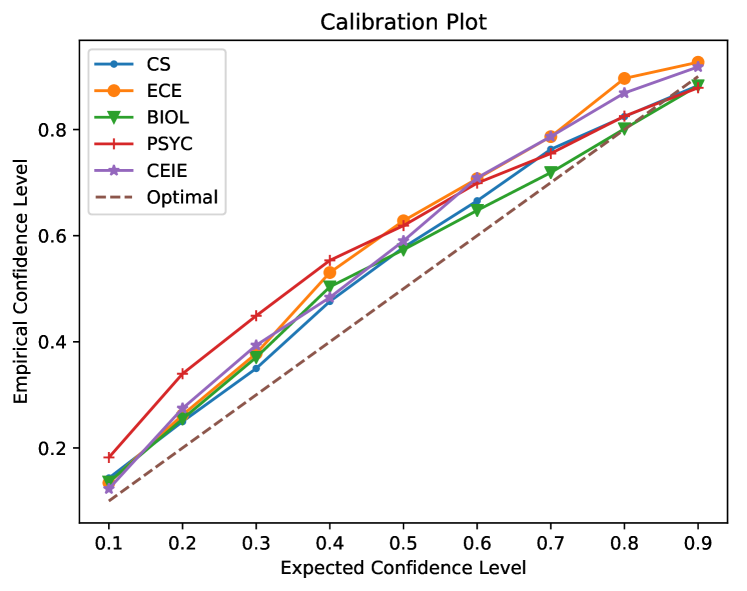
Figure 3. Empirical confidence level vs. expected confidence level

The second way to evaluate uncertainty estimation is that a model should make less errors on predictions that it is confident about. Therefore, we evaluate the model as a function of confidence score and we propose error@k:

$$E@k=\text{error}(\text{k most confident predictions}),$$

where error can be mean absolute error or tick error, the predictions are ranked in terms of predictive variance, lower predictive variance is more confident. Figure 4 shows mean absolute error with respect to top-k confident predictions. The figure shows that as the predictions become less confident, the prediction errors become higher.

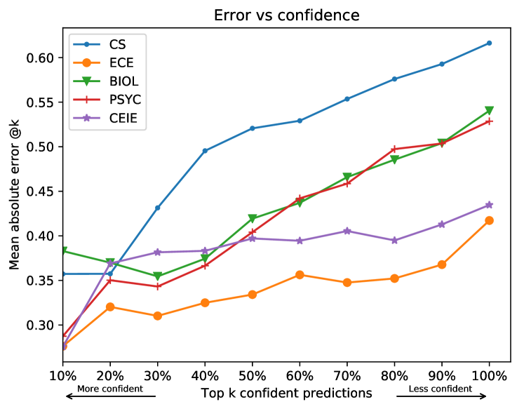
Figure 4. MAE as a function of confidence.

Grade prediction is fundamental for early-warning student facing system. The application case of educational early-warning system is that when an instructor/advisor is informed that a student will fail a course, the instructor will reach out to the student and provide the student personalized advising and help. In this process, we want to make sure students who are not failing are not predicted as failing students (false positives) so as to reduce wasted educational resources; and the failing students are not predicted as passing students (false negatives) so that they can get much needed timely help. Prediction confidence is useful for reducing these kind of errors by only taking action on confident predictions. We also evaluate uncertainty estimation on the application of identification of at-risk students. Figure 5 shows false negative rate (FNR) and false positive rate (FPR) as a function of prediction confidence.

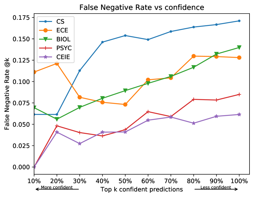
(a) FNR vs confidence

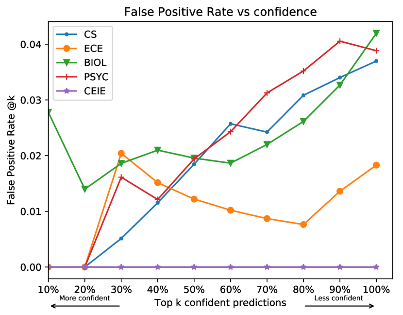
(b) FPR vs confidence

Figure 5. FNR and FPR as a function of prediction confidence

We observe in most cases as prediction confidence decreases, there are more errors. To make less errors, we can choose to take actions only on confident predictions. However, more confident predictions have less coverage. In practice, we propose to set an appropriate confidence threshold to make a tradeoff between coverage and accuracy. All the uncertainties are estimated by using MLP and we levae uncertainty estimation using LSTM to future work.

5.4. Case Studies: Influential Courses

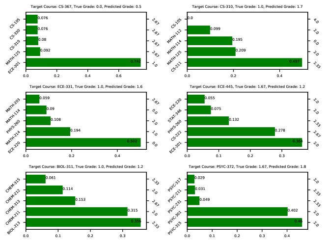
Figure 6. Influence of prior courses. For every subfigure, x-axis is influence value, left y-axis is top five most influential prior courses, right y-axis is student’s grade in corresponding prior course. In the titles, target course means the course for which we are predicting grade, predicted grade is the predicted grade for the student, and true grade is the student’s real grade in the target course.

To incorporate the developed next-term grade approaches within personalized advising system, we seek to not only report the predicted grades for the student but identify the list of prior courses that were most influential for determining future success in a given target course.

Figure 6 shows examples of use case scenarios for students in different disciplines. We choose six at-risk students from CS, ECE, BIOL and PSYCH majors. If a student has grade lower than 2.0, he/she is identified as at-risk student. We compute the influence of the prior courses on the prediction as described in Section 3.5 and only prior courses contributing to the increase in the prediction are reported. The influence is computed by using the LSTM model. The influence index is sorted and normalized and only the top five prior courses are shown in the table. From the top left subfigure, we can see that the student’s true grade in class CS-367 (this course is about computer systems and programming) is 0.0, the predicted grade is 0.5 and the most influential prior course is ECE-301 (class about digital electronics) which is a prerequisite. The influence of a prior course is computed by increasing the grade of that course to full grade (i.e. 4.0). This does not suggest that a course with a lower grade has higher influence than a course with higher grade. For example, in top right subfigure, the lowest grade of the student is from MATH-114 (about calculus), but the most influential is course CS-211 (about object-oriented programming) (prerequisite of the target course). The left column of second row shows the third example. The target course is ECE-331 (about digital system design). For this student, the actual grade in the target course is 1.0 and predicted grade is 1.6. The most influential course is ECE-220 (about signals and systems), as this student performed very poorly in this course (grade was 0.0). From the results, we can see that the proposed approach is able to identify influential prior courses that explain the prediction results.

Target Course Top 5 Influential Prior Courses CS-367 ECE-301 CS-310 MATH-125 CS-262 MATH-213 ECE-433 ECE-333 MATH-203 STAT-346 PHYS-160 ENGR-107 PSYC-372 PSYC-325 PSYC-301 PSYC-300 PSYC-211 PSYC-100 BIOL-311 BIOL-213 CHEM-211 CHEM-212 CHEM-313 BIOL-214 CEIE-331 PHYS-261 CEIE-210 STAT-344 PHYS-161 MATH-113

Table 6. Top 5 influential prior courses for a target course. Bolded course is the pre-requisite.

Table 6 shows the influence of prior courses on a target course for groups of students. We choose five representative courses from each major. From the table, we observe that for all the courses their prerequisites are one of the top five most influential courses. Although, most of the time, the most influential prior course for a target course is not necessarily the prerequisite, the most influential course is very relevant to the target course. For example, course CS-367 about low-level computer system such as machine-level programming; the most influential course ECE-301 is digital electronics, which is about designing logic circuits and relevant to low-level computer system. Providing a list of influential courses for a target course can help stakeholders improve the curriculum and program structure.

6. Conclusions

In this work, we proposed two course-specific Bayesian deep learning models for next-term grade prediction. The first is a multi-layer perceptron which treats the feature vector as static and ignores the temporal dynamics of a student’s knowledge evolution. To overcome this issue, we also developed a Long Short Term Memory model that takes into account the sequential aspect of student’s knowledge accumulating process by taking courses across semester/terms.

We highlight the strengths of our proposed approach by incorporating the predictions within three application scenarios: (i) identify at-risk students and (ii) provide explainable results so as to identify a list of influential courses associated with a target course. (iii) provide prediction uncertainty for building a reliable educational early warning system.

We conducted comprehensive experiments to evaluate the proposed models. The experiments demonstrate that the proposed models exhibit better performance at predicting students’ grades than state-of-the-art baselines. The experiments also show that the proposed models have better capability at identifying at-risk students.

- (1)
- Agrawal et al. (2014) Rakesh Agrawal, Maria Christoforaki, Sreenivas Gollapudi, Anitha Kannan, Krishnaram Kenthapadi, and Adith Swaminathan. 2014. Mining videos from the web for electronic textbooks. In International Conference on Formal Concept Analysis. Springer, 219–234.
- Al-Barrak and Al-Razgan (2016) Mashael A Al-Barrak and Muna Al-Razgan. 2016. Predicting students final GPA using decision trees: a case study. International Journal of Information and Education Technology 6, 7 (2016), 528.
- Anschuetz (2015) Nika Anschuetz. 2015. Breaking the 4-year myth: Why students are taking longer to graduate? http://college.usatoday.com/2015/12/16/breaking-the-4-year-myth-why-students-are-taking-longer-to-graduate/
- Arnold (1957) Vladimir I Arnold. 1957. On functions of three variables. In Dokl. Akad. Nauk SSSR, Vol. 114. 679–681.
- Avati et al. (2017) Anand Avati, Kenneth Jung, Stephanie Harman, Lance Downing, Andrew Ng, and Nigam H Shah. 2017. Improving palliative care with deep learning. arXiv preprint arXiv:1711.06402 (2017).
- Benjamin (2014) Aaron Benjamin. 2014. Factors Influencing Learning. (2014).
- Bydžovská (2015a) Hana Bydžovská. 2015a. Are collaborative filtering methods suitable for student performance prediction?. In Portuguese Conference on Artificial Intelligence. Springer, 425–430.
- Bydžovská (2015b) Hana Bydžovská. 2015b. Student performance prediction using collaborative filtering methods. In International Conference on Artificial Intelligence in Education. Springer, 550–553.
- Corbett and Anderson (1994) Albert T Corbett and John R Anderson. 1994. Knowledge tracing: Modeling the acquisition of procedural knowledge. User modeling and user-adapted interaction 4, 4 (1994), 253–278.
- Elbadrawy and Karypis (2016) Asmaa Elbadrawy and George Karypis. 2016. Domain-aware grade prediction and top-n course recommendation. In Proceedings of the 10th ACM Conference on Recommender Systems. ACM, 183–190.
- Elbadrawy et al. (2016) Asmaa Elbadrawy, Agoritsa Polyzou, Zhiyun Ren, Mackenzie Sweeney, George Karypis, and Huzefa Rangwala. 2016. Predicting student performance using personalized analytics. Computer 49, 4 (2016), 61–69.
- Gal and Ghahramani (2015) Yarin Gal and Zoubin Ghahramani. 2015. On modern deep learning and variational inference. In Advances in Approximate Bayesian Inference workshop, NIPS, Vol. 2.
- Gal and Ghahramani (2016) Yarin Gal and Zoubin Ghahramani. 2016. Dropout as a Bayesian approximation: Representing model uncertainty in deep learning. In international conference on machine learning. 1050–1059.
- Gedeon and Turner (1993) TD Gedeon and S Turner. 1993. Explaining student grades predicted by a neural network. In Neural Networks, 1993. IJCNN’93-Nagoya. Proceedings of 1993 International Joint Conference on, Vol. 1. IEEE, 609–612.
- Hochreiter and Schmidhuber (1997) Sepp Hochreiter and Jürgen Schmidhuber. 1997. Long short-term memory. Neural computation 9, 8 (1997), 1735–1780.
- Hu et al. (2017) Qian Hu, Agoritsa Polyzou, George Karypis, and Huzefa Rangwala. 2017. Enriching Course-Specific Regression Models with Content Features for Grade Prediction. (2017).
- Kingma and Ba (2014) Diederik P Kingma and Jimmy Ba. 2014. Adam: A method for stochastic optimization. arXiv preprint arXiv:1412.6980 (2014).
- Kolmogorov (1963) Andrei Nikolaevich Kolmogorov. 1963. On the representation of continuous functions of many variables by superposition of continuous functions of one variable and addition. Translations American Mathematical Society 2, 28 (1963), 55–59.
- Koren et al. (2009) Yehuda Koren, Robert Bell, and Chris Volinsky. 2009. Matrix factorization techniques for recommender systems. Computer 42, 8 (2009).
- Lan et al. (2014) Andrew S Lan, Andrew E Waters, Christoph Studer, and Richard G Baraniuk. 2014. Sparse factor analysis for learning and content analytics. The Journal of Machine Learning Research 15, 1 (2014), 1959–2008.
- LeCun et al. (2015) Yann LeCun, Yoshua Bengio, and Geoffrey Hinton. 2015. Deep learning. nature 521, 7553 (2015), 436.
- Li et al. (2016) Jiwei Li, Will Monroe, and Dan Jurafsky. 2016. Understanding neural networks through representation erasure. arXiv preprint arXiv:1612.08220 (2016).
- Livieris et al. (2012) Ioannis E Livieris, Konstantina Drakopoulou, and Panagiotis Pintelas. 2012. Predicting students’ performance using artificial neural networks. In 8th PanHellenic Conference with International Participation Information and Communication Technologies in Education. 321–328.
- Mangal (2002) SK Mangal. 2002. Advanced educational psychology. PHI Learning Pvt. Ltd.
- OKUBO et al. ([n. d.]) Fumiya OKUBO, Takayoshi YAMASHITA, Atsushi SHIMADA, and Shin’ichi KONOMI. [n. d.]. Students’ Performance Prediction Using Data of Multiple Courses by Recurrent Neural Network. ([n. d.]).
- Piech et al. (2015) Chris Piech, Jonathan Bassen, Jonathan Huang, Surya Ganguli, Mehran Sahami, Leonidas J Guibas, and Jascha Sohl-Dickstein. 2015. Deep knowledge tracing. In Advances in Neural Information Processing Systems. 505–513.
- Polyzou and Karypis (2016a) Agoritsa Polyzou and George Karypis. 2016a. Grade prediction with course and student specific models. In Pacific-Asia Conference on Knowledge Discovery and Data Mining. Springer, 89–101.
- Polyzou and Karypis (2016b) Agoritsa Polyzou and George Karypis. 2016b. Grade prediction with models specific to students and courses. International Journal of Data Science and Analytics 2, 3-4 (2016), 159–171.
- Ren et al. (2017) Zhiyun Ren, Xia Ning, and Huzefa Rangwala. 2017. Grade Prediction with Temporal Course-wise Influence. arXiv preprint arXiv:1709.05433 (2017).
- Ribeiro et al. (2016) Marco Tulio Ribeiro, Sameer Singh, and Carlos Guestrin. 2016. Why should i trust you?: Explaining the predictions of any classifier. In Proceedings of the 22nd ACM SIGKDD International Conference on Knowledge Discovery and Data Mining. ACM, 1135–1144.
- Rosenblatt (1961) Frank Rosenblatt. 1961. Principles of neurodynamics. perceptrons and the theory of brain mechanisms. Technical Report. CORNELL AERONAUTICAL LAB INC BUFFALO NY.
- Sorour et al. (2015) Shaymaa E Sorour, Kazumasa Goda, and Tsunenori Mine. 2015. Student Performance Estimation Based on Topic Models Considering a Range of Lessons. In International Conference on Artificial Intelligence in Education. Springer, 790–793.
- Stillwell and Sable (2013) Robert Stillwell and Jennifer Sable. 2013. Public School Graduates and Dropouts from the Common Core of Data: School Year 2009-10. First Look (Provisional Data). NCES 2013-309. National Center for Education Statistics (2013).
- Sweeney et al. (2016) Mack Sweeney, Huzefa Rangwala, Jaime Lester, and Aditya Johri. 2016. Next-term student performance prediction: A recommender systems approach. arXiv preprint arXiv:1604.01840 (2016).
- Umair and Sharif (2018) Sajid Umair and Muhammad Majid Sharif. 2018. Predicting Students Grades Using Artificial Neural Networks and Support Vector Machine. In Encyclopedia of Information Science and Technology, Fourth Edition. IGI Global, 5169–5182.
- Yang et al. (2017) Tsung-Yen Yang, Christopher G Brinton, Carlee Joe-Wong, and Mung Chiang. 2017. Behavior-Based Grade Prediction for MOOCs Via Time Series Neural Networks. IEEE Journal of Selected Topics in Signal Processing 11, 5 (2017), 716–728.
- Yudelson et al. (2013) Michael V Yudelson, Kenneth R Koedinger, and Geoffrey J Gordon. 2013. Individualized bayesian knowledge tracing models. In International Conference on Artificial Intelligence in Education. Springer, 171–180.