Brownian motion tree models are toric

Abstract.

Felsenstein’s classical model for Gaussian distributions on a phylogenetic tree is shown to be a toric variety in the space of concentration matrices. We present an exact semialgebraic characterization of this model, and we demonstrate how the toric structure leads to exact methods for maximum likelihood estimation. Our results also give new insights into the geometry of ultrametric matrices.

1. Introduction

Brownian motion tree models are classical statistical models for phylogenetic trees. They were introduced by Felsenstein [Fel73] to examine continuous measurements of phenotypes in evolutionary biology. The vertices of the tree represent real-valued random variables, whose joint distribution obeys a Gaussian law.

Let $\tilde{T}$ be a tree with $n+1$ leaves, labelled $0,1,\ldots,n$, and with no vertices of degree two. Let $T$ be the rooted tree obtained from $\tilde{T}$ by directing all edges away from $0$. The set $V$ of non-root vertices of $T$ is in natural bijection with the set of edges of $T$. A vertex $u\in V$ is a descendant of $v\in V$ if there is a directed path from $v$ to $u$. The set of all leaves of $T$ that are descendants of $v$ is denoted by ${\rm de}(v)$. We fix a total order on $V$ such that $u\leq v$ if ${\rm de}(u)\subseteq{\rm de}(v)$. Given $u,v\in V$, we write $w={\rm lca}(u,v)$ for their most recent common ancestor. Figure 1 shows our running example.

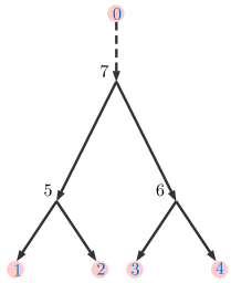
Figure 1. A tree $T$ with $n{=}4$ leaves, $|V|{=}7$ edges, and its matrix representation.

In the space $\mathbb{S}^{n}$ of symmetric $n\times n$ matrices $\Sigma=(\sigma_{ij})$ we consider the subspace

$$\mathcal{L}_{T}\;=\;\bigl{\{}\,\Sigma\in\mathbb{S}^{n}:\;\sigma_{ij}=\sigma_{kl}\,\mbox{ if }\,{\rm lca}(i,j)={\rm lca}(k,l)\,\bigr{\}}.$$

Using parameters $(t_{v}:v\in V)$, the matrices in $\mathcal{L}_{T}$ satisfy $\sigma_{ij}=t_{v}$ for $v={\rm lca}(i,j)$. This furnishes a representation of the tree $T$ by a matrix, as shown in Figure 1.

We are interested in Gaussian distributions on $\mathbb{R}^{n}$ with covariance matrix in $\mathcal{L}_{T}$. Their concentration matrices $K=(\kappa_{ij})$ form the $|V|$-dimensional algebraic variety

$$\mathcal{L}_{T}^{-1}\,\,=\,\,\bigl{\{}\,K=\Sigma^{-1}\,:\,\Sigma\in\mathcal{L}_{T}\,\bigr{\}}\quad\subset\,\,\,\mathbb{S}^{n}.$$

We identify $\mathcal{L}_{T}^{-1}$ with its Zariski closure in the projective space $\mathbb{P}(\mathbb{S}^{n})\simeq\mathbb{P}^{\binom{n+1}{2}-1}$. In this paper we show that the variety $\mathcal{L}_{T}^{-1}$ is linearly isomorphic to a toric variety in $\mathbb{P}^{\binom{n+1}{2}-1}$. In tropical geometry [MS15, Remark 4.3.11] and algebraic combinatorics [BFF18, Theorem 4.6], one associates a toric ideal $I_{\tilde{T}}$ with the unrooted tree ${\tilde{T}}$ as follows. The ideal $I_{\tilde{T}}$ has the quadratic generators $p_{ik}p_{jl}-p_{il}p_{jk}$ where $\{i,j\}$ and $\{k,l\}$ are cherries in the induced $4$-leaf subtree on any quadruple $i,j,k,l\in\{0,1,\ldots,n\}$.

To reveal the toric structure, we introduce a change of coordinates in $\mathbb{S}^{n}$ as follows:

(1) $$\begin{matrix}p_{ij}&=&-\kappa_{ij}\quad&\quad{\rm for}\,\,1\leq i<j\leq n,\\ p_{0i}&=&\sum_{j=1}^{n}\kappa_{ij}&{\rm for}\,\,1\leq i\leq n.\end{matrix}$$

With this, the concentration matrix $K=(\kappa_{ij})$ is the reduced Laplacian of the complete graph on $n{+}1$ vertices with edge labels $p_{ij}$. See [MSUZ16, Example 4.9], where the matrix for $n=3$ is shown in equation (4.6). Here is the same scenario for $n=4$:

Example 1.1.

We fix coordinates $\,p_{01},p_{02},\ldots,p_{34}\,$ on $\,\mathbb{P}(\mathbb{S}^{4})=\mathbb{P}^{9}\,$ by setting

$$\small K\,\,=\,\,\begin{bmatrix}p_{01}{+}p_{12}{+}p_{13}{+}p_{14}\!&-p_{12}&-p_{13}&-p_{14}\\ -p_{12}&\!p_{02}{+}p_{12}{+}p_{23}{+}p_{24}\!&-p_{23}&-p_{24}\\ -p_{13}&-p_{23}&\!p_{03}{+}p_{13}{+}p_{23}{+}p_{34}\!&-p_{34}\\ -p_{14}&-p_{24}&-p_{34}&\!p_{04}{+}p_{14}{+}p_{24}{+}p_{34}\end{bmatrix}\!.$$

Fix the tree $T$ in Figure 1. The $6$-dimensional toric variety $\mathcal{L}_{T}^{-1}$ in $\mathbb{P}^{9}$ is defined by

$$I_{\tilde{T}}\,=\,\langle\,p_{01}p_{23}-p_{02}p_{13},\,p_{01}p_{24}-p_{02}p_{14},\,p_{03}p_{14}-p_{04}p_{13},\,p_{03}p_{24}-p_{04}p_{23},\,p_{13}p_{24}-p_{14}p_{23}\,\rangle.$$

These quadrics vanish for the inverse of any matrix with the structure in Figure 1. ∎

The title of this paper is an abridged version of the following statement:

Theorem 1.2.

The variety $\mathcal{L}^{-1}_{T}$ of concentration matrices in the Brownian motion tree model, in coordinates (1), coincides with the toric variety defined by the ideal $I_{\tilde{T}}$.

The proof of this theorem will be given in Section 3. First, however, in Section 2, we offer an introduction to the statistical model and its phylogenetic applications. Our statistical models correspond to semialgebraic subsets of $\mathcal{L}_{T}$ or $\mathcal{L}^{-1}_{T}$. We are interested in two subsets of $\mathcal{L}_{T}$, namely the spectrahedron $\mathcal{L}_{T}\,\cap\,\mathbb{S}_{+}^{n}$, obtained by intersection with the cone $\,\mathbb{S}_{+}^{n}\,$ of positive definite matrices, and the polyhedral cone

$$\mathcal{L}_{T,\geq}\;=\;\ \bigl{\{}\,\Sigma\in\mathcal{L}_{T}:\;0\leq\sigma_{ij}\leq\sigma_{kl}\,\mbox{ whenever}\,{\rm lca}(i,j)\leq{\rm lca}(k,l)\bigr{\}}.$$

We shall see that $\mathcal{L}_{T,\geq}$ is a simplicial cone, contained in the spectrahedron $\mathcal{L}_{T}\cap\mathbb{S}_{+}^{n}$.

Matrices in $\mathcal{L}_{T,\geq}$ play an important role in statistics. By Proposition 3.14 in [DMSM14], every matrix $\Sigma$ in $\mathcal{L}_{T,\geq}$ is an ultrametric matrix in $\mathbb{S}^{n}$, i.e. it satisfies $\,\sigma_{ij}\geq\min\{\sigma_{ik},\sigma_{jk}\}\geq 0\,$ for all $i,j,k$. By Theorem 3.16, every ultrametric matrix lies in $\mathcal{L}_{T,\geq}$ for some tree $T$. Ultrametric matrices appear in the potential theory of finite state Markov chains, which is the context of [DMSM14]. Our motivation came from phylogenetics [Fel73] and Gaussian maximum likelihood estimation [ZUR17].

Every matrix $\Sigma$ in $\mathbb{S}_{+}^{n}$ represents a Gaussian distribution on $\mathbb{R}^{n}$. Both $\mathcal{L}_{T}\cap\mathbb{S}_{+}^{n}$ and $\mathcal{L}_{T,\geq}$ belong to the class of linear Gaussian covariance models [And70, ZUR17].

The main result of this paper is Theorem 2.6. This is an extension of Theorem 1.2 which features toric inequalities $p_{ik}p_{jl}\leq p_{ij}p_{kl}$ in addition to the quadratic binomial equations in $I_{\tilde{T}}$. It offers an exact semialgebraic description of the model $\mathcal{L}_{T,\geq}^{-1}$ in terms of the nonnegative coordinates $p_{ij}$. The proof of this result is presented in Section 5. It rests on formulas that express $p_{ij}$ in terms of treks as in [STD10].

Section 4 is about fitting Brownian motion tree models to data, given by a sample covariance matrix $S$ in $\mathbb{S}^{n}_{+}$. We do so by maximizing the log-likelihood function

(2) $$\ell(\Sigma)\;=\;-\log\det\Sigma-{\rm trace}(S\Sigma^{-1}).$$

This function is non-convex. The expression in terms of $K=\Sigma^{-1}$ equals

(3) $$\ell(K)\;=\;\log\det K-{\rm trace}(SK).$$

This function is convex in $K$, which motivates analyzing maximum likelihood estimation for Brownian motion tree models as an optimization problem over $\mathcal{L}_{T}^{-1}$. As we will show in Section 4, in this parameterization maximum likelihood estimation boils down to solving a system of polynomial equations on $\mathcal{L}_{T}^{-1}$. The paper concludes with a brief discussion on how Theorem 2.6 might be applied to likelihood inference.

2. Tree models and their parameters

Brownian motion is a stochastic process that characterizes the random motion of particles. It is a Wiener process $W_{t}$ satisfying $W_{0}=0$, with independent increments, and such that $W_{t}-W_{s}$ for $t\geq s$ has a Gaussian distribution with mean zero and variance $t-s$. Brownian motion on a rooted binary tree $T$ can also be described using the Wiener process. The process starts at vertex $0$. At time $t=t_{2n-1}$, it splits into two, and each of the two processes starts evolving independently at value $W_{t_{2n-1}}$. It again proceeds according to the Wiener process until another splitting event occurs. We think about this process as evolving along $T$, where the parameters $t_{v}$ for inner vertices $v$ represent the times of splitting events. This construction is a continuous interpretation of the Gaussian structural equation model (4) discussed next.

Given a rooted tree $T$, we define a Gaussian distribution on $T$ as follows. First, set $Y_{0}\equiv 0$. Then to each vertex $v\in V$ we associate independently a Gaussian random variable $\epsilon_{v}$ with mean zero and variance $\theta_{v}\geq 0$. The corresponding Markov process on $T$ is a collection of real-valued random variables $Y_{v}$ for $v\in V$. They satisfy

(4) $$Y_{v}=Y_{u}+\epsilon_{v}\quad\mbox{for every edge }\,u\to v\in E.$$

Since a linear transformation of a Gaussian vector is also Gaussian, we conclude that the random vector $Y=(Y_{v})_{v\in V}$ is Gaussian. The set of covariance matrices of the marginal distributions on the leaf-variables $(Y_{1},\ldots,Y_{n})$ is the polyhedral cone $\mathcal{L}_{T,\geq}$.

Proposition 2.1.

The random vector $(Y_{1},\ldots,Y_{n})$ is normally distributed with mean zero, and the entries $\sigma_{ij}={\rm cov}(Y_{i},Y_{j})$ of its covariance matrix $\Sigma_{\theta}$ are

(5) $$\sigma_{ij}\,\,\;=\;\sum_{v\leq{\rm lca}(i,j)}\theta_{v}\qquad{\rm for}\,\,i,j=1,\ldots,n.$$

The resulting Gaussians on $\mathbb{R}^{n}$ are precisely those with covariance matrices in $\mathcal{L}_{T,\geq}$.

Proof..

Using (4) recursively, we can write each $Y_{i}$ in terms of the error terms as

$$Y_{i}\,\,=\,\,\sum_{v\leq i}\epsilon_{v}.$$

Equation (5) follows from this and the fact that all $\epsilon$’s are mutually independent. The linear inequalities $\,\sigma_{ij}\leq\sigma_{kl}\,$ that define the polyhedral cone $\mathcal{L}_{T,\geq}$ inside the linear space $\mathcal{L}_{T}$ are equivalent to the requirement that the $\theta_{i}$’s be nonnegative. ∎

Example 2.2.

Consider the tree in Figure 1. The random variables for the inner vertices of the tree are $Y_{0}=0$, $Y_{7}=\epsilon_{7}$, $Y_{5}=\epsilon_{7}+\epsilon_{5}$, $Y_{6}=\epsilon_{7}+\epsilon_{6}$, and we have $\,Y_{1}=\epsilon_{7}+\epsilon_{5}+\epsilon_{1},\;Y_{2}=\epsilon_{7}+\epsilon_{5}+\epsilon_{2},\;Y_{3}=\epsilon_{7}+\epsilon_{6}+\epsilon_{3},\;Y_{4}=\epsilon_{7}+\epsilon_{6}+\epsilon_{4}\,$ for the leaves.

The $\epsilon_{v}$ are independent univariate Gaussians with mean $0$ and variance $\theta_{v}$. Hence the marginal distribution of $(Y_{1},Y_{2},Y_{3},Y_{4})$ is Gaussian with the covariance matrix

(6) $$\small\Sigma_{\theta}\,\,=\,\,\begin{bmatrix}\theta_{1}+\theta_{5}+\theta_{7}&\theta_{5}+\theta_{7}&\theta_{7}&\theta_{7}\\ \theta_{5}+\theta_{7}&\theta_{2}+\theta_{5}+\theta_{7}&\theta_{7}&\theta_{7}\\ \theta_{7}&\theta_{7}&\theta_{3}+\theta_{6}+\theta_{7}&\theta_{6}+\theta_{7}\\ \theta_{7}&\theta_{7}&\theta_{6}+\theta_{7}&\theta_{4}+\theta_{6}+\theta_{7}\end{bmatrix}.$$

This is the matrix in (5) and in Figure 1. The constraint that the $\theta_{i}$ are nonnegative translates into the inequalities $t_{1},t_{2}\geq t_{5}$ and $t_{3},t_{4}\geq t_{6}$ and $t_{5},t_{6}\geq t_{7}\geq 0$. ∎

The extreme rays of the polyhedral cone $\mathcal{L}_{T,\geq}$ are as follows. Let $g_{v}\in\{0,1\}^{n}$ be the vector with $(g_{v})_{i}=1$ if $i\in{\rm de}(v)$ and $(g_{v})_{i}=0$ otherwise. The corresponding rank one matrices $G_{v}=g_{v}g_{v}^{T}$ form a basis for $\mathcal{L}_{T}$. In fact, the matrix in (5) equals

(7) $$\Sigma\;=\;\sum_{v\in V}\theta_{v}G_{v}.$$

Corollary 2.3.

The cone $\mathcal{L}_{T,\geq}$ is a simplicial cone, spanned by the rank one matrices $G_{v}$ associated with vertices $v\in V$. It is contained in the spectrahedral cone $\mathcal{L}_{T}\cap\mathbb{S}_{+}^{n}$.

Note that this inclusion is strict. For instance, the matrix $\Sigma_{\theta}$ in (6) is positive definite if we set $\,\theta_{1}=\theta_{2}=\theta_{3}=\theta_{4}=5$, $\theta_{5}=\theta_{6}=0$ and $\theta_{7}=-1$. This means that the linear covariance model is strictly larger than the Brownian motion tree model.

We next interpret our model in the context of distance-based phylogenetics. Using the natural bijection between non-root vertices and edges, we label each edge of $T$ with a parameter $\theta_{v}$. This is shown in the tree on the right in Figure 1. We think of $\theta_{v}\geq 0$ as the length of the associated edge. We compute the distance between any two leaves of $\tilde{T}$ by summing the lengths of edges on the unique path joining them. The collection of resulting distances $d_{ij}$ for $i,j=0,1,\ldots,n$ is a tree metric on $\tilde{T}$.

The correspondence between ultrametric $n\times n$ matrices and tree metrics on $n+1$ taxa is known in phylogenetics as the Farris transform. The formulas are

$$\left\{\begin{array}[]{ll}\sigma_{ii}\;\;=\;\;d_{0i}&\mbox{for }1\leq i\leq n\\ \sigma_{ij}\;\;=\;\;\frac{1}{2}(d_{0i}+d_{0j}-d_{ij})&\mbox{for }1\leq i<j\leq n,\end{array}\right.$$

and these are equivalent to (5). The inverse of the Farris transform is given by

$$\left\{\begin{array}[]{ll}d_{0i}\;\;=\;\;\sigma_{ii}&\mbox{for }1\leq i\leq n\\ d_{ij}\;\;=\;\;\sigma_{ii}+\sigma_{jj}-2\sigma_{ij}&\mbox{for }1\leq i\leq j\leq n.\end{array}\right.$$

Proposition 2.4.

The model $\mathcal{L}_{T,\geq}$ is identified with the cone of tree metrics on $\tilde{T}$ via the Farris transform $(d_{ij})\mapsto(\sigma_{ij})$. The parameters $\theta_{v}$ are the lengths of the edges.

Proof..

The diagonal entry $\sigma_{ii}$ of the covariance matrix is the sum of the lengths $\theta_{v}$ of the incoming edges for all vertices $v$ on the path from the root $0$ to leaf $i$. Therefore, $d_{0i}=\sigma_{ii}$ is the distance from $0$ to $i$ in the unrooted tree $\tilde{T}$. Each off-diagonal entry $\sigma_{ij}$ is the length of the path from the root $0$ to ${\rm lca}(i,j)$. Hence $\sigma_{ii}-\sigma_{ij}$ is the length of the path from ${\rm lca}(i,j)$ to the leaf $i$. We conclude that $d_{ij}=(\sigma_{ii}-\sigma_{ij})+(\sigma_{jj}-\sigma_{ij})$ is the length of the path from leaf $i$ to leaf $j$ in $\tilde{T}$. Since the Farris transform is an invertible linear transformation, it identifies the two simplicial cones in $\mathbb{R}^{\binom{n+1}{2}}$. ∎

We next turn to the space of all tree metrics, which is a key object in phylogenetics. A classical result of Buneman [Bun71] states that a metric $D=(d_{ij})$ on $\{0,\ldots,n\}$ is a tree metric (for some tree) if and only if it satisfies the four point condition:

(8) $$d_{ij}+d_{kl}\;\leq\;\max\{d_{ik}+d_{jl},d_{il}+d_{jk}\}\quad\hbox{for all $\,i,j,k,l\in\{0,1,\ldots,n\}$.}$$

If $D$ is a tree metric on $\tilde{T}$ then the following additional equation holds:

(9) $$\quad d_{ik}+d_{jl}\;=\;d_{il}+d_{jk}\qquad\hbox{if $\{i,j\},\,\{k,l\}$ are cherries in the quartet on $i,j,k,l$}.$$

The constraints (8) and (9) are well-known also in tropical geometry [MS15, §4.3] where one identifies the space of tree metrics with the tropical Grassmannian that parametrizes tropical lines in $\mathbb{R}^{n+1}/\mathbb{R}{\bf 1}$. This is related to Theorem 1.2 as follows.

Remark 2.5.

If we set $p_{ij}=e^{-d_{ij}}$ then the linear relations (9) that hold for tree metrics on ${\tilde{T}}$ are precisely the equations $p_{ik}p_{jk}=p_{il}p_{jk}$ that define the toric ideal $I_{\tilde{T}}$.

We now state our main result. It augments Theorem 1.2 by incorporating the inequalities in (8). The unrooted tree obtained from $\tilde{T}$ by restricting to any four leaves $i,j,k,l$ is called a quartet of $\tilde{T}$. If equality holds in (8) then this four-leaf tree is a star quartet. If the inequality in (8) is strict then we call it a trivalent quartet.

Theorem 2.6.

Given any rooted tree $T$, the set $\mathcal{L}_{T,\geq}^{-1}$ of concentration matrices in the Brownian motion tree model is the set of positive definite matrices $K$ satisfying

(10) $$\begin{matrix}&p_{ij}\,\geq\,0&\hbox{for all}\quad 0\leq i<j\leq n,\\ &p_{ik}p_{jl}\;=\;p_{il}p_{jk}\;=\;p_{ij}p_{kl}&\hbox{for all star quartets}\,\,\,ijkl,\\ \hbox{and}\quad&p_{ik}p_{jl}\;=\;p_{il}p_{jk}\;\leq\;p_{ij}p_{kl}&\quad\hbox{for all trivalent quartets}\,\,\,ij|kl.\end{matrix}$$

Remark 2.7.

These inequalities are satisfied by $p_{ij}=e^{-d_{ij}}$ where $(d_{ij})$ is any tree metric on $\tilde{T}$. Thus, the set of models $\mathcal{L}_{T,\geq}^{-1}$, where $T$ ranges over all rooted trees on $n$ leaves, is a multiplicative realization of the space of phylogenetic trees. This is reminiscent of the space of phylogenetic oranges studied by Moulton and Steel [MS04].

We illustrate the contents of Theorem 2.6 for our running example.

Example 2.8.

Fix the tree in Figure 1 with covariance matrix $\Sigma_{\theta}$ in (6). Set $s:={\rm det}(\Sigma_{\theta})>0$. Writing the concentration matrix $K=\Sigma_{\theta}^{-1}$ as in Example 1.1, we have

$$\small\begin{matrix}p_{13}s\,=\,\theta_{2}\theta_{4}\theta_{7},\,\,p_{14}s\,=\,\theta_{2}\theta_{3}\theta_{7},\,\,p_{23}s\,=\,\theta_{1}\theta_{4}\theta_{7},\,\,p_{24}s\,=\,\theta_{1}\theta_{3}\theta_{7},\,\,(p_{03}p_{12}-p_{02}p_{13}){s}=\theta_{4}\theta_{5},\\ (p_{04}p_{12}-p_{02}p_{14}){s}\,=\,\theta_{3}\theta_{5}\,,\,\,\,(p_{01}p_{34}-p_{04}p_{13}){s}\,=\,\theta_{2}\theta_{6}\,,\,\,\,(p_{02}p_{34}-p_{04}p_{23}){s}\,=\,\theta_{1}\theta_{6}\,,\vskip 3.0pt plus 1.0pt minus 1.0pt\\ (p_{12}p_{34}-p_{14}p_{23}){s}\,=\,\theta_{5}\theta_{6}+\theta_{5}\theta_{7}+\theta_{6}\theta_{7}\,,\\ p_{01}s\,=\,(\theta_{3}\theta_{4}+\theta_{3}\theta_{6}+\theta_{4}\theta_{6})\theta_{2}\,,\quad p_{02}s\,=\,(\theta_{3}\theta_{4}+\theta_{3}\theta_{6}+\theta_{4}\theta_{6})\theta_{1}\,,\\ p_{03}s\,=\,(\theta_{1}\theta_{2}+\theta_{1}\theta_{5}+\theta_{2}\theta_{5})\theta_{4}\,,\quad p_{04}s\,=\,(\theta_{1}\theta_{2}+\theta_{1}\theta_{5}+\theta_{2}\theta_{5})\theta_{3}\,,\\ p_{12}s\,=\,\theta_{3}\theta_{4}\theta_{5}+\theta_{3}\theta_{4}\theta_{7}+\theta_{3}\theta_{5}\theta_{6}+\theta_{3}\theta_{5}\theta_{7}+\theta_{3}\theta_{6}\theta_{7}+\theta_{4}\theta_{5}\theta_{6}+\theta_{4}\theta_{5}\theta_{7}+\theta_{4}\theta_{6}\theta_{7}\,,\\ p_{34}s\,=\,\theta_{1}\theta_{2}\theta_{6}+\theta_{1}\theta_{2}\theta_{7}+\theta_{1}\theta_{5}\theta_{6}+\theta_{1}\theta_{5}\theta_{7}+\theta_{1}\theta_{6}\theta_{7}+\theta_{2}\theta_{5}\theta_{6}+\theta_{2}\theta_{5}\theta_{7}+\theta_{2}\theta_{6}\theta_{7}.\end{matrix}$$

The five quadratic binomials in $I_{\tilde{T}}$ are zero for these $p_{ij}$. Assuming this, Theorem 2.6 says that these $15$ expressions are nonnegative if and only if $\theta_{1},\ldots,\theta_{7}\geq 0$.

3. Toric ideals from trees

In this section we prove Theorem 1.2. The proof of Theorem 2.6 is given in Section 5. The following code in Macaulay2 [M2] provides the quadratic generators for our running example. It also shows that the rooted tree $T$ need not be binary.

Example 3.1.

Example 1.1 can be verified in Macaulay2 [M2] by running this code:

R = QQ[t1,t2,t3,t4,t5,t6,t7,p01,p02,p03,p04,p12,p13,p14,p23,p24,p34];
S = matrix {{t1,t5,t7,t7},
            {t5,t2,t7,t7},
            {t7,t7,t3,t6},
            {t7,t7,t6,t4}};
K = matrix {{p01+p12+p13+p14, -p12, -p13, -p14},
            {-p12, p02+p12+p23+p24, -p23, -p24},
            {-p13, -p23, p03+p13+p23+p34, -p34},
            {-p14, -p24, -p34, p04+p14+p24+p34}};
id4 = matrix {{1,0,0,0},{0,1,0,0},{0,0,1,0},{0,0,0,1}};
I = eliminate({t1,t2,t3,t4,t5,t6,t7},minors(1,S*K-id4))
codim I, degree I, betti mingens I

As claimed, the toric ideal has codimension $3$, degree $5$ and five quadratic generators.

We now examine non-binary trees. First we replace the two occurrences of t6 by t7 in the covariance matrix S. The resulting tree has $|V|=6$. By running the modified Macaulay2 code, we see that the ideal is still toric. It has codimension $4$, degree $8$ and 7 quadratic generators. Finally, we replace both t5 and t6 with t7. Now the unrooted tree $\tilde{T}$ has $|V|=5$. It is the star tree with leaves $0,1,2,3,4$. Its toric ideal $I_{\tilde{T}}$ is the ideal of the second hypersimplex. It has codimension $5$ and degree $11$, with 10 quadratic generators. Modifying the code confirms these data. ∎

Proof of Theorem 1.2.

We use the following parametric representation for the toric variety of the ideal $I_{\tilde{T}}$ associated with the unrooted tree ${\tilde{T}}$. It is given by Laurent monomials in the entries $t_{v}$ of the matrix representation of the rooted tree $T$:

(11) $$\begin{matrix}p_{ij}&\mapsto&t_{{\rm lca}(i,j)}/(t_{i}t_{j})&\quad{\rm for}\,\,1\leq i<j\leq n,\\ p_{0i}&\mapsto&1/t_{i}&{\rm for}\,\,1\leq i\leq n.\end{matrix}$$

The ideal $I_{\tilde{T}}$ is the kernel of the ring homomorphism $\mathbb{R}[p]\rightarrow\mathbb{R}[t^{\pm}]$ given by (11).

The variety $\mathcal{L}_{T}^{-1}$ is a cone in $\mathbb{S}^{n}$ given parametrically by mapping a covariance matrix $\Sigma$ to its inverse $K=\Sigma^{-1}$. Since the parametrization is homogeneous, we may replace the inverse by the adjoint. By slight abuse of notation we set $K={\rm det}(\Sigma)\cdot\Sigma^{-1}$. The entries $\kappa_{ij}$ of the matrix $K$ are homogeneous polynomials of degree $n-1$ in the parameters $t=(t_{v})$ for $v\in V$. The same holds for the coordinates $p_{ij}$ in (1). We write $P_{ij}(t)$ for these homogeneous polynomials. Our claim states that the toric ideal $I_{\tilde{T}}$ coincides with the kernel of the ring homomorphism $\mathbb{R}[p]\rightarrow\mathbb{R}[t],\,p_{ij}\mapsto P_{ij}(t)$.

To prove this, we examine the initial monomials and the irreducible factorization of the polynomials $P_{ij}(t)$. Here we fix the degree reverse lexicographic order on $\mathbb{R}[t]$ given by $t_{u}\succ t_{v}$ if $u\leq v$ in $T$. For $1\leq i<j\leq n$, the polynomial $P_{ij}(t)$ is equal (up to sign) to the determinant of the $(n-1)\times(n-1)$ submatrix of $\Sigma$ that is obtained by deleting row $i$ and column $j$. The initial monomial is the product of the entries of that submatrix which appear along the main diagonal. To be precise, we find

$${\rm in}(P_{ij}(t))\,\,=\,\,t_{1}t_{2}\cdots t_{n}\cdot t_{{\rm lca}(i,j)}/(t_{i}t_{j}).$$

The polynomial $P_{0i}(t)$ is the determinant of the $n\times n$ matrix obtained from $\Sigma$ by replacing the $i$th row with the all-ones vector $(1,1,\ldots,1)$. Its initial monomial equals

$${\rm in}(P_{0i}(t))\,\,=\,\,t_{1}t_{2}\cdots t_{n}\cdot(1/t_{i}).$$

Hence, by (11), the relations among the initial monomials are precisely given by $I_{\tilde{T}}$. We claim that each of the quadratic binomial relations among the above Laurent monomials lifts to exactly the same relation among the full polynomials $P_{ij}(t)$ and $P_{0i}(t)$. We shall prove this by examining the factorizations of these polynomials.

In what follows we first assume that $T$ is a binary tree, i.e. every vertex in $V\backslash\{1,2,\ldots,n\}$ has precisely two children in $T$. At the end of the proof, we shall derive Theorem 1.2 for non-binary trees from the same statement for binary trees.

For any inner vertex $k$ in the rooted binary tree $T$, let $T_{k}$ denote the rooted tree obtained from $T$ by deleting all edges and vertices below $k$. Thus $T_{k}$ is a rooted tree with leaves $\{k\}\cup(\{1,\ldots,n\}\backslash{\rm de}(k))$. Let $D_{k}(t)$ denote the determinant of its covariance matrix. This is a homogeneous polynomial of degree $n+1-|{\rm de}(k)|$. For any directed edge $u\rightarrow v$ of the tree $T$, we consider the submatrix of $\Sigma$ with row indices ${\rm de}(u)\backslash{\rm de}(v)$ and column indices $({\rm de}(u)\backslash{\rm de}(v))\cup\{k\}$, for any fixed $\,k\in{\rm de}(v)$. This matrix does not depend on $k$, and it has one more column than rows. We make it square by placing the all-ones vector $(1,\ldots,1)$ into the first row. We write $E_{uv}(t)$ for the determinant of that square matrix. This is a homogeneous polynomial in $(t_{v})_{v\in V}$ of degree $|{\rm de}(u)\backslash{\rm de}(v)|$. By convention, $E_{0v}=1$ for the root edge $0\to v$.

Consider the path between any two leaves $i$ and $j$ in the unrooted tree $\tilde{T}$. Each vertex $u$ in the interior of such a path has a unique child $v$ in the rooted tree $T$ that is not on the path. Here we are using the assumption that $T$ is a binary tree. The only exception is the top vertex $u={\rm lca}(i,j)$ on the path between $i$ and $j$ in $T$.

We find that the polynomial $P_{0i}(t)$ is equal to the product of all determinants $E_{uv}(t)$ where $u\rightarrow v$ is any edge on the path from $0$ to $i$. Similarly, the $(n-1)\times(n-1)$ determinant $P_{ij}(t)$ is equal to $D_{{\rm lca}(i,j)}(t)$ times the product of all $E_{uv}(t)$ where the vertex $u\not={\rm lca}(i,j)$ is on the path from leaf $i$ to leaf $j$. One verifies this by examining for which parameter values $t$ these expressions vanish, and by noting that the initial monomials coincide with the products of the initial monomials of the factors:

$$\begin{matrix}{\rm in}(D_{k}(t))&=&t_{k}\cdot\prod\{t_{i}\,:\,i\in\{1,\ldots,n\}\backslash{\rm de}(k)\},\\ {\rm in}(E_{uv}(t))&=&\prod\{t_{i}\,:\,i\in{\rm de}(v)\}.\end{matrix}$$

The above factorizations of $P_{0i}(t)$ and $P_{ij}(t)$ into the determinants $D_{\bullet}(t)$ and $E_{\bullet}(t)$ show that each generator $p_{ik}p_{jl}-p_{il}p_{jk}$ of $I_{\tilde{T}}$ vanishes on our variety. By our analysis of the leading monomials, there are no relations among the polynomials $P_{ij}(t)$ and $P_{0i}(t)$ beyond those in $I_{\tilde{T}}$. In fact, our analysis shows that these polynomials form a Khovanskii basis (cf. [KM19]) for the reverse lexicographic monomial order on the $t_{i}$.

We now know that Theorem 1.2 holds for all binary trees. It remains to derive from this the same statement for all non-binary trees. The property for rooted trees to be binary translates into the property for unrooted trees to be trivalent. Let $\tilde{T}$ be any non-trivalent tree and let $[\tilde{T}]$ be the set of all trivalent trees $\tilde{U}$ that are obtained by refining $\tilde{T}$. One verifies that the following identity among toric ideals holds:

(12) $$I_{\mathcal{\tilde{T}}}\quad=\quad\sum_{\tilde{U}\in[\tilde{T}]}I_{\tilde{U}}.$$

Similarly, the linear space $\mathcal{L}_{T}$ is the intersection of all the linear spaces $\mathcal{L}_{U}$, where $\tilde{U}$ runs over $[\tilde{T}]$. Since matrix inversion is a birational isomorphism, the variety $\mathcal{L}_{T}^{-1}$ is the intersection of the toric varieties $\mathcal{L}_{U}^{-1}$ where $\tilde{U}$ runs over the trivalent trees in $[\tilde{T}]$. The Nullstellensatz implies that the sum of toric ideals (12) cuts out $\mathcal{L}_{T}^{-1}$ set-theoretically. This shows that $\mathcal{L}_{T}^{-1}$ is a toric variety, with toric ideal in (12). ∎

Example 3.2.

Consider the binary tree in Figure 1 and Examples 1.1 and 3.1. The special determinants defined above are the following polynomials:

$$E_{51}=t_{2}-t_{5}\,,\,\,E_{52}=t_{1}-t_{5}\,,\,\,E_{63}=t_{4}-t_{6}\,,\,\,E_{64}=t_{3}-t_{6}\,,$$

$$\small E_{75}\,\,=\,\,{\rm det}\begin{bmatrix}1&1&1\\ t_{7}&t_{3}&t_{6}\\ t_{7}&t_{6}&t_{4}\end{bmatrix},\quad E_{76}\,\,=\,\,{\rm det}\begin{bmatrix}1&1&1\\ t_{1}&t_{5}&t_{7}\\ t_{5}&t_{2}&t_{7}\end{bmatrix}.$$

We are interested in the projective variety in $\mathbb{P}^{9}$ that is parametrized by

$$\begin{matrix}p_{01}\,=\,E_{75}E_{51},\,\,p_{02}\,=\,E_{75}E_{52},\,\,p_{03}\,=\,E_{76}E_{63},\,\,p_{04}\,=\,E_{76}E_{64},\,\,p_{12}\,=\,D_{5},\,\,p_{34}\,=\,D_{6},\\ p_{13}\,=\,E_{51}D_{7}E_{63},\,\,\,p_{14}\,=\,E_{51}D_{7}E_{64},\,\,\,p_{23}\,=\,E_{52}D_{7}E_{63},\,\,\,p_{24}\,=\,E_{52}D_{7}E_{64}.\end{matrix}$$

One verifies that this is the variety defined by the toric ideal $I_{\tilde{T}}$ seen in Example 1.1. Furthermore, the same toric variety is also parametrized by the initial monomials ${\rm in}(p_{01})=t_{2}t_{3}t_{4},\,{\rm in}(p_{02})=t_{1}t_{3}t_{4},\,\ldots\,,\,{\rm in}(p_{24})=t_{1}t_{3}t_{7}$, and $\,{\rm in}(p_{34})=t_{1}t_{2}t_{6}$. ∎

Remark 3.3.

Tropical geometers know that the toric ideals $I_{\tilde{T}}$ are precisely the monomial-free initial ideals of the Plücker ideal that defines the Grassmannian of lines. The latter arises in a manner that is similar to our passage from covariance matrices to concentration matrices, namely by inverting matrices $\Sigma$ that have a Hankel structure. This is the content of [MSUZ16, Proposition 7.2]. We do not know whether this is related to the present paper. Is it possible to derive Theorem 1.2 by a degeneration argument from the relationship between Hankel matrices $\Sigma$ and Bézout matrices $K$?

4. Maximum likelihood algebra

The log-likelihood function for Gaussian random variables is the function $\ell(\Sigma)$ in (2). Here $S=(s_{ij})$ is a fixed sample covariance matrix, i.e. $S=\frac{1}{N}XX^{T}$ where $X$ is a real $n\times N$ matrix whose columns are the observed samples. Maximum likelihood estimation is concerned with maximizing the expression (2) over all covariance matrices $\Sigma=(\sigma_{ij})$ in the model of interest. This optimization problem is equivalent to maximizing the expression (3) over all concentration matrices $K$ in the model.

The optimal solution to this problem is denoted by $\hat{\Sigma}=({\hat{\sigma}}_{ij})$ or $\hat{K}=({\hat{\kappa}}_{ij})$. This is called the maximum likelihood estimate (MLE) for the data $S$. Here the model is fixed but the data $S$ can vary. We therefore think of the MLE as a function of $S$.

In this section we study the MLE for the Brownian motion tree model $\mathcal{L}_{T,\geq}$. The idea is to take advantage of the toric structure revealed in Theorem 1.2. Thus, we use the coordinate change (1) that writes the concentration matrix $K$ as the reduced Laplacian for the complete graph on $n+1$ vertices with edge labels $p_{ij}$. With this, the expression (3) is a function of the $p_{ij}$, subject to the toric constraints in $I_{\tilde{T}}$. This gives us the flexibility to choose a convenient parametrization of the toric variety.

In algebraic statistics, one distinguishes two kinds of polynomial constraints for a statistical model, namely equations and inequalities. It is customary to first focus on the equations and examine the MLE in that setting before incorporating inequalities.

In our paper, the model is given by the semialgebraic set $\mathcal{L}_{T,\geq}^{-1}$. This set satisfies the inequalities in Theorem 2.6. For the discussion of MLE in the current section, we ignore the inequality constraints and identify the set $\mathcal{L}_{T,\geq}^{-1}$ with its Zariski closure, which is the toric variety $\mathcal{L}_{T}^{-1}=\mathcal{V}(I_{\tilde{T}})$. The critical points of the likelihood function $\ell(K)$ on that variety are defined by a system of polynomial equations, known in statistics as the likelihood equations. These can be derived by using Lagrange multipliers, or via a monomial parametrization of the toric variety $\mathcal{V}(I_{\tilde{T}})$.

The maximum likelihood degree of the model is, by definition, the number of complex solutions to the likelihood equations for generic data $S$. This number is an algebraic invariant of the ideal $I_{\tilde{T}}$. To compute it we take $S$ to be a general symmetric $n\times n$ matrix of full rank $n$ and we count all complex critical points of $\ell(K)$.

Proposition 4.1.

The maximum likelihood degree of the Brownian motion tree model on a binary tree $\tilde{T}$ with $\,n=2,3,4,5,6,7,8\,$ leaves is equal to $\,1,1,5,17,61,233,917$.

Proof..

This result was found by symbolic computation, namely using the Gröbner basis package in the computer algebra system maple. For $n\geq 6$ the computation was carried out over a finite field. All combinatorial types of trees were considered. See Example 4.4 for an illustration of the case $n=4$ where the ML degree is $5$. ∎

This result is complementary to the usual approach in computational statistics where one maximizes the likelihood function using a local numerical method, such as the Newton-Raphson algorithm. Local methods perform best in a regime where the likelihood function is concave. Such a regime was identified in [ZUR17], where concavity was shown to hold with high probability when the dimension $n$ is small relative to the sample size $N$. In that analysis it was essential to use all constraints of the model, i.e., not just the equations but also the inequalities.

The maximum likelihood degree being equal to one means that the MLE can be written as a rational function of the data. Proposition 4.1 says that this happens for our model when $n=2$ and $n=3$. We next present the formulas for these two cases.

Example 4.2 ($n=2$).

The toric ideal $I_{\tilde{T}}$ equals $\{0\}$, so our model is the full Gaussian family. This means that the MLE equals the sample covariance matrix:

$$\hat{\sigma}_{11}=s_{11},\,\,\hat{\sigma}_{12}=s_{12},\,\,\hat{\sigma}_{22}=s_{22}.$$

Since the MLE of the parameters is $\hat{t}_{1}=s_{11}$, $\hat{t}_{2}=s_{22}$, $\hat{t}_{3}=s_{12}$, this leads to valid parameters for the Brownian motion tree model if $\min\{s_{11},s_{22}\}\geq s_{12}\geq 0$. ∎

Example 4.3 ($n=3$).

We label the rooted tree $T$ so that $\{1,2\}$ is a clade. Hence $\{1,2\}$ and $\{0,3\}$ are the cherries in the unrooted tree $\tilde{T}$. Our toric ideal is principal:

$$I_{\tilde{T}}\,=\,\langle p_{01}p_{23}-p_{02}p_{13}\rangle\,=\,\langle\kappa_{11}\kappa_{23}-\kappa_{12}\kappa_{13}+\kappa_{12}\kappa_{23}-\kappa_{13}\kappa_{22}\rangle.$$

This is equivalent to setting $\sigma_{13}=\sigma_{23}$ in the covariance matrix $\Sigma=K^{-1}$. The MLE is a rational function of the entries $s_{ij}$ of the sample covariance matrix $S$. We define

$$c\,=\,(s_{11}-2s_{12}+s_{22})s_{33}-(s_{13}-s_{23})^{2}.$$

The entries $\hat{\sigma}_{ij}$ of the estimated covariance matrix $\hat{\Sigma}$ satisfy $\,\hat{\sigma}_{33}=s_{33}\,$ and

$$\begin{matrix}\hat{\sigma}_{11}&\!=\!&s_{11}-2(s_{13}{-}s_{23})(s_{11}s_{33}{-}s_{12}s_{33}{-}s_{13}^{2}{+}s_{13}s_{23})(s_{11}s_{23}{-}s_{12}s_{13}{-}s_{12}s_{23}{+}s_{13}s_{22})/c^{2},\\ \hat{\sigma}_{12}&\!=\!&s_{12}-\,(s_{13}{-}s_{23})(s_{11}s_{33}{-}s_{13}^{2}{-}s_{22}s_{33}{+}s_{23}^{2})(s_{11}s_{23}-s_{12}s_{13}-s_{12}s_{23}+s_{13}s_{22})/c^{2},\\ \hat{\sigma}_{22}&\!=\!&s_{22}-2(s_{13}{-}s_{23})(s_{12}s_{33}{-}s_{13}s_{23}{-}s_{22}s_{33}{+}s_{23}^{2})(s_{11}s_{23}{-}s_{12}s_{13}{-}s_{12}s_{23}{+}s_{13}s_{22})/c^{2}.\end{matrix}$$

The remaining two matrix entries must be equal:

$$\begin{matrix}&\hat{\sigma}_{13}&=&s_{13}-(s_{13}-s_{23})(s_{11}s_{33}-s_{13}^{2}-s_{12}s_{33}+s_{13}s_{23})/c\\ =&\hat{\sigma}_{23}&=&s_{23}-(s_{23}-s_{13})(s_{22}s_{33}-s_{23}^{2}-s_{12}s_{33}+s_{13}s_{23})/c.\end{matrix}$$

The following two linear forms are preserved when passing from data to MLE:

$$\hat{\sigma}_{11}-2\hat{\sigma}_{12}+\hat{\sigma}_{22}\;=\;s_{11}-2s_{12}+s_{22}\qquad{\rm and}\qquad\hat{\sigma}_{33}=s_{33}.$$

Writing $K=(k_{ij})=S^{-1}$ for the sample concentration matrix, we note that $K-\hat{K}$ is a rank $2$ matrix which depends only on $s_{33}$, $s_{13}-s_{23}$, and $s_{11}-2s_{12}+s_{22}$. Also, $c\;=\;(k_{11}+2k_{12}+k_{22})/{\rm det}(K).$ ∎

Example 4.4 ($n=4$).

We consider the tree $\tilde{T}$ in Figure 1. Its toric variety $\mathcal{V}(I_{\tilde{T}})=\mathcal{L}_{T}^{-1}\subset\mathbb{P}^{9}$ was discussed in Examples 1.1, 3.1 and 3.2. We shall prove that the MLE for this model cannot be expressed in radicals. For this, we fix the parametrization

(13) $$\begin{matrix}p_{01}=u_{1},\,p_{02}=u_{2},\,p_{03}=u_{3},\,p_{04}=u_{4},\,\,p_{12}=u_{1}u_{2}u_{6},\,p_{13}=u_{1}u_{3}u_{5},\,\\ \qquad\quad p_{14}=u_{1}u_{4}u_{5},\,\,\,p_{23}=u_{2}u_{3}u_{5},\,\,\,p_{24}=u_{2}u_{4}u_{5},\,\,\,p_{34}=u_{3}u_{4}u_{7}.\end{matrix}$$

We substitute this into the concentration matrix $K$ in Example 1.1. The determinant of that $4\times 4$ matrix is a polynomial of degree $10$ with $81$ terms:

$${\rm det}(K)\,=\,u_{1}^{4}u_{2}u_{3}u_{4}u_{5}^{2}u_{6}+3u_{1}^{3}u_{2}^{2}u_{3}u_{4}u_{5}^{2}u_{6}+u_{1}^{3}u_{2}u_{3}^{2}u_{4}u_{5}^{3}+\,\cdots\,+u_{1}u_{2}u_{3}u_{4}^{2}u_{7}+u_{1}u_{2}u_{3}u_{4}.$$

For our computation we now take the sample covariance matrix

(14) $$\small S\,\,=\,\,\begin{bmatrix}5&3&1&2\\ 3&5&1&1\\ 1&1&5&3\\ 2&1&3&4\\ \end{bmatrix}.$$

Thus ${\rm trace}(SK)=4u_{1}u_{2}u_{6}+8u_{1}u_{3}u_{5}+\cdots+5u_{3}+4u_{4}$. Our goal is to maximize the likelihood function $\log(\det(K))-{\rm trace}(SK)$ where $(u_{1},u_{2},\ldots,u_{7})$ ranges over $\mathbb{R}^{7}$. Its seven partial derivatives are rational functions in the $u_{j}$. We clear denominators and impose ${\rm det}(K)\not=0$. This results in a system of polynomial equations. We fix the lexicographic term order with $u_{1}>u_{2}>\cdots>u_{7}$, we compute the reduced Gröbner basis in maple, and we find that it has a triangular shape. For $i=1,2,\ldots,6$, the Gröbner basis has an element $u_{i}-p_{i}(u_{7})$, where $p_{i}$ is a univariate polynomial of degree six with large rational coefficients. In addition, we see the quintic polynomial

(15) $$\small\quad\begin{matrix}5955844829180400\,u_{7}^{5}\,-\,203897411425749580\,u_{7}^{4}\,+\,129689372089999498\,u_{7}^{3}\\ -\,139971736881354888\,u_{7}^{2}\,+\,44907572962723196\,u_{7}\,-\,5517030143672333.\end{matrix}$$

This polynomial has precisely one real root at $\hat{u}_{7}=33.607528...$. By back-substitution, we compute the estimated concentration matrix $\widehat{K}$, and we find its inverse to be

$$\small\widehat{\Sigma}\,=\begin{bmatrix}4.757115029565996&\!3.040016668717226&\!1.418803877886187&\!1.418803877886187\\ 3.040016668717226&\!5.322918307868457&\!1.418803877886187&\!1.418803877886187\\ 1.418803877886187&\!1.418803877886187&\!5.295621559259030&\!3.094192269251272\\ 1.418803877886187&\!1.418803877886187&\!3.094192269251272&\!3.892762979243514\end{bmatrix}\!\!.$$

Note that this matrix lies in $\mathcal{L}_{T,\leq}$, so it is the true MLE for the statistical model.

Using maple, we also check that the Galois group of the polynomial (15) over the rational numbers $\mathbb{Q}$ is the symmetric group on $5$ letters. Hence $\hat{u}_{7}$ cannot be written in radicals over $\mathbb{Q}$. This implies that the MLE cannot be written in radicals. ∎

Proposition 4.1 only applies to rooted trees $T$ that are binary. This raises the question what happens for degenerate tree topologies. At first glance, one might think that the ML degree decreases for special trees. However, this is not the case:

Example 4.5 ($n=4$ revisited).

Let $\tilde{T}$ be the star tree on five leaves, so $T$ is the directed tree obtained from the tree in Figure 1 by shrinking the edges labeled $\theta_{5}$ and $\theta_{6}$. Recall from Example 3.1 that $I_{\tilde{T}}$ has codimension $5$ and degree $11$. It has $10$ quadratic generators. We obtain a parametrization by setting $u_{5}=u_{6}=u_{7}$ in (13).

Performing the same computation as in Example 4.4, we find that the ML degree of this star tree model is 21. For the sample covariance matrix $S$ in (14), we find

$$\small\widehat{\Sigma}\,=\begin{bmatrix}2.945585253871356&3.350776006974025&3.350776006974025&3.350776006974025\\ \!3.350776006974025&\!5.654229276230780&\!3.350776006974025&\!3.350776006974025\\ \!3.350776006974025&\!3.350776006974025&\!\!11.10861203686456&\!3.350776006974025\\ \!3.350776006974025&\!3.350776006974025&\!3.350776006974025&\!5.509927633167128\end{bmatrix}\!\!.$$

The matrix entries in $\widehat{\Sigma}$ are algebraic numbers of degree 21 over $\mathbb{Q}$. ∎

In the case of star trees, the MLE problem can be formulated via (2) as follows:

• Minimize $\,\log(\det\Sigma)-{\rm trace}(S\Sigma^{-1})\,$ over the set of symmetric matrices $\Sigma\in\mathbb{S}^{n}_{+}$ whose off-diagonal entries are equal and smaller than the diagonal entries.

We obtained the following result concerning the algebraic degree of this optimization problem. Just like Proposition 4.1, this was found using computations with maple.

Proposition 4.6.

The maximum likelihood degree of the Brownian motion star tree model with $\,n=2,3,4,5,6,7,8,9\,$ is equal to $\,\delta_{n}=1,7,21,51,113,239,493,1003$.

It is natural to conjecture that this degree always satisfies $\,\delta_{n+1}=2(\delta_{n}+n)+1$.

Remark 4.7.

The estimated matrix $\widehat{\Sigma}$ in Example 4.5 lies in the spectrahedron $\mathcal{L}_{T}\cap\mathbb{S}^{4}_{+}$. It is not in the model $\mathcal{L}_{T,\geq}$ for the star tree $\tilde{T}$ because the upper left entry is smaller than the off-diagonal entry in the first row. This discrepancy motivates studying the inequalities in Theorem 2.6, whose proof is given in the next  section.

5. Being on trek in semialgebraic statistics

Our goal is to prove that the inequalities in Theorem 2.6 are valid for our model. Namely, we show that $p_{ij}$ and $p_{ij}p_{kl}-p_{il}p_{jk}$ are nonnegative on $\mathcal{L}_{T,\geq}$. This is done by applying the theory of treks due to Sullivant, Talaska and Draisma [STD10].

A symmetric $n\times n$ matrix $K$ is an M-matrix if $K$ is positive definite and $\kappa_{ij}\leq 0$ for all $i\neq j$. Moreover, $K$ is diagonally dominant if $|\kappa_{ii}|\geq\sum_{j\neq i}|\kappa_{ij}|$ for all $i$. If $K$ is an M-matrix then it is diagonally dominant if and only if the vector $K\mathbf{1}$ has nonnegative entries. Therefore, a matrix $K=[\kappa_{ij}]$ is a diagonally dominant M-matrix if and only $K\in\mathbb{S}^{n}_{+}$ and the quantities $p_{ij}=-\kappa_{ij}$ and $p_{0i}=\sum_{j=1}^{n}\kappa_{ij}$ in (1) are nonnegative.

It is known in linear algebra [VN93, Theorem 2.2] that the inverse of any symmetric ultrametric matrix is a diagonally dominant M-matrix. This explains why all points in $\mathcal{L}_{T,\geq}^{-1}$ have nonnegative coordinates. This constraint is the first in (10). The validity of the other inequality constraints arises from the following key lemma.

Lemma 5.1.

The determinant ${\rm det}(\Sigma)$ times the quantity $\,p_{ij}p_{kl}-p_{il}p_{jk}\,$ in (10) is a sum of products of parameters $\theta_{i}$, so it is nonnegative when the $\theta_{i}$ are nonnegative.

The proof of this lemma is given below. The case $n=4$ was seen in Example 2.8. To provide some intuition, we now prove Lemma 5.1 and Theorem 2.6 for $n\leq 3$.

Example 5.2 ($n\leq 3$).

Let $n=2$. There are no constraints in (10), and we have

$$\small K\,=\,\Sigma^{-1}\;\;=\;\;\begin{bmatrix}\theta_{1}+\theta_{3}&\theta_{3}\\ \theta_{3}&\theta_{2}+\theta_{3}\end{bmatrix}^{-1}\;\;=\;\;\frac{1}{\theta_{1}\theta_{2}+\theta_{1}\theta_{3}+\theta_{2}\theta_{3}}\begin{bmatrix}\theta_{2}+\theta_{3}&-\theta_{3}\\ -\theta_{3}&\theta_{1}+\theta_{3}\end{bmatrix}.$$

Assuming that $K$ lies in $\mathbb{S}^{2}_{+}$, then the vector $(p_{01},p_{02},p_{03})$ is nonnegative if and only if $(\theta_{1},\theta_{2},\theta_{3})={\rm det}(\Sigma){\cdot}(p_{02},p_{01},p_{12})$ is nonnegative. This proves Theorem 2.6 for $n=2$.

Let $n=3$ and $T$ be the binary tree with clade $\{1,2\}$. Theorem 2.6 asserts that the model $\mathcal{L}_{T,\geq}^{-1}$ is equal to the set of all diagonally dominant M-matrices satisfying

(16) $$p_{01}p_{23}\;=\;p_{02}p_{13}\;\leq\;p_{03}p_{12}.$$

The former is contained in the latter because a direct calculation reveals that

(17) $$p_{01}\det\Sigma=\theta_{2}\theta_{3},\quad p_{02}\det\Sigma=\theta_{1}\theta_{3},\quad p_{03}\det\Sigma=\theta_{1}\theta_{2}+\theta_{1}\theta_{4}+\theta_{2}\theta_{4},$$

$$p_{12}\det\Sigma=\theta_{3}\theta_{4}+\theta_{3}\theta_{5}+\theta_{4}\theta_{5},\quad p_{13}\det\Sigma=\theta_{2}\theta_{5},\quad p_{23}\det\Sigma=\theta_{1}\theta_{5},$$

$$(p_{03}p_{12}-p_{01}p_{23})\det\Sigma\;=\;\theta_{4}.$$

Conversely, let $K$ be a diagonally dominant M-matrix satisfying (16). By Theorem 1.2, the equation in (16) implies that $K\in\mathcal{L}_{T}^{-1}$. Since $K$ is invertible, we can define $\Sigma=K^{-1}$. Then $\Sigma=\Sigma_{\theta}$ for some real vector $(\theta_{1},\ldots,\theta_{5})$ that satisfies (17). From (16) we obtain $\theta_{4}\geq 0$. Nonnegativity of $p_{0i},p_{ij}$ implies that $\theta_{1},\theta_{2},\theta_{3},\theta_{5}$ are either all nonpositive or all nonnegative. We want to show that they are all nonnegative. Suppose they are negative. Since $p_{03}\det\Sigma\geq 0$ and $p_{12}\det\Sigma\geq 0$, we have

$$\theta_{4}\;\leq\;-\frac{\theta_{1}\theta_{2}}{\theta_{1}+\theta_{2}},\qquad\theta_{4}\;\leq\;-\frac{\theta_{3}\theta_{5}}{\theta_{3}+\theta_{5}}.$$

However, $\,\det\Sigma\;=\;\theta_{4}(\theta_{1}+\theta_{2})(\theta_{3}+\theta_{5})+\theta_{1}\theta_{2}(\theta_{3}+\theta_{5})+(\theta_{1}+\theta_{2})\theta_{3}\theta_{5}\;>\;0\,$ and so

$$\theta_{4}\;>\;-\frac{\theta_{1}\theta_{2}}{\theta_{1}+\theta_{2}}-\frac{\theta_{3}\theta_{5}}{\theta_{3}+\theta_{5}}.$$

This is a contradiction and hence Theorem 2.6 holds for $n\leq 3$. ∎

Fix the tree $T$ with $n$ leaves as before. A trek from leaf $i$ to leaf $j$ is a pair $\gamma=(P_{L},P_{R})$, where $P_{L}$ is a directed path from some vertex $v$ to $i$ and $P_{R}$ is a directed path from $v$ to $j$. The leaf $i$ is the initial vertex, the leaf $j$ is the final vertex, and $v=v(\gamma)$ is the top of the trek. The parameter $\theta_{v(\gamma)}$ is the weight of the trek. We also allow treks between $i=0$ and $j$, in which case the associated weight is $1$. Given two sets $A$ and $B$ with the same cardinality, a trek system $\Gamma$ from $A$ to $B$ consists of $|A|$ treks whose initial vertices exhaust the set $A$ and whose final vertices exhaust the set $B$. The weight of a trek system is the product of the weights of all its treks.

In our application either $A=\{1,\ldots,n\}\backslash\{j\}$ and $B=\{1,\ldots,n\}\backslash\{i\}$ if $1\leq i\leq j\leq n$, or $A=\{0,1,\ldots,n\}\backslash\{j\}$ and $B=\{1,\ldots,n\}$ if $0=i<j\leq n$. We assume that all treks are mutually vertex-disjoint. Equivalently, we consider the set $\mathcal{T}_{i,j}$ of trek systems $\Gamma$ from $A$ to $B$ that consist of the following $|A|$ vertex-disjoint treks:

1. one trek from $i$ to $j$,

2. $|A\cap B|$ treks from $k$ to $k$ for each $k\in A\cap B$.

In Figure 2 we display the set $\mathcal{T}_{1,2}$ for our running example. Its elements are the eight trek systems from $A=\{1,3,4\}$ to $B=\{2,3,4\}$ in the tree $T$ shown in Figure 1.

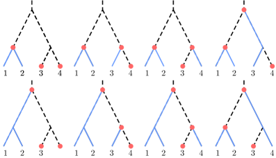
Figure 2. Eight trek systems from $A=\{1,3,4\}$ to $B=\{2,3,4\}$. Treks are indicated by solid edges. Dots mark the tops of the treks.

Proposition 5.3.

The following identity holds for all indices $\,0\leq i<j\leq n$:

$$p_{ij}\det\Sigma\;=\;\sum_{\Gamma\in\mathcal{T}_{i,j}}\prod_{\gamma\in\Gamma}\theta_{v(\gamma)}$$

Moreover, each monomial appears in this sum only once.

Proof..

We first prove the second assertion: each trek system in $\mathcal{T}_{i,j}$ gives a different monomial. Suppose there are two different trek systems $\Gamma$, $\Gamma^{\prime}$ such that $\prod_{\gamma\in\Gamma}\theta_{v(\gamma)}=\prod_{\gamma\in\Gamma^{\prime}}\theta_{v(\gamma)}$. Let $\gamma,\gamma^{\prime}$ be two treks in $\Gamma,\Gamma^{\prime}$ with the initial point $k$ and the final point $l$ (either $k=l$ or $k=i$, $l=j$). Both $v(\gamma)$ and $v(\gamma^{\prime})$ lie on the path between $0$ and ${\rm lca}(k,l)$. If $v(\gamma)\neq v(\gamma^{\prime})$ then one lies above the other, say $v(\gamma)<v(\gamma^{\prime})$. But then $v(\gamma^{\prime})$ lies on the trek of $\Gamma$ from $k$ to $l$ and so it cannot be at the top of another trek in $\Gamma$ because treks must be mutually disjoint. This leads to a contradiction unless $\gamma=\gamma^{\prime}$. We conclude that $\Gamma=\Gamma^{\prime}$.

We now prove the main formula. Consider first the case $1\leq i\leq j\leq n$. We have

$$\kappa_{ij}\det\Sigma\;=\;(-1)^{i+j}\det\Sigma_{A,B},$$

where $A=\{1,\ldots,n\}\backslash\{j\}$ and $B=\{1,\ldots,n\}\backslash\{i\}$. Let $\Lambda=[\lambda_{uv}]\in\{0,1\}^{V\times V}$ be the matrix with $\lambda_{uv}=1$ if $u\to v$ in $T$ and $\lambda_{uv}=0$ otherwise, and let $D_{\theta}$ be the diagonal matrix with entries $\theta=(\theta_{v})$. The covariance matrix of the model (4) equals

$$\Xi\;\;=\;\;(I-\Lambda)^{-T}D_{\theta}(I-\Lambda)^{-1}.$$

The principal submatrix of $\Xi$ corresponding to the leaves of $T$ is $\Sigma$. Hence $\det\Sigma_{A,B}=\det\Xi_{A,B}$. Every trek system between $A$ and $B$ gives rise to a permutation $\pi\in S_{n-1}$ and we define ${\rm sign}(\Gamma):={\rm sign}(\pi)$. If $\Gamma\in\mathcal{T}_{i,j}$ then ${\rm sign}(\pi)=(-1)^{i+j+1}$ unless $i=j$ in which case $\pi$ is the identity. Using equation (2) in [DST13], we conclude that

$$\det\Sigma_{A,B}\;=\;\begin{cases}\phantom{-}\sum_{\Gamma\in\mathcal{T}_{i,i}}\prod_{\gamma\in\Gamma}\theta_{v(\gamma)}&\mbox{if }i=j,\\ -\sum_{\Gamma\in\mathcal{T}_{i,j}}(-1)^{i+j}\prod_{\gamma\in\Gamma}\theta_{v(\gamma)}&\mbox{if }i\neq j.\end{cases}$$

The formula in [DST13] involves all trek systems between $A$ and $B$, but the sum can be restricted to trek systems with no sided intersections [DST13, Definition 3.2]. In our case this is equivalent to treks being mutually vertex-disjoint. It follows that

$$\kappa_{ij}\det\Sigma\;=\;\begin{cases}\phantom{-}\sum_{\Gamma\in\mathcal{T}_{i,i}}\prod_{\gamma\in\Gamma}\theta_{v(\gamma)}&\mbox{if }i=j,\\ -\sum_{\Gamma\in\mathcal{T}_{i,j}}\prod_{\gamma\in\Gamma}\theta_{v(\gamma)}&\mbox{if }i\neq j.\end{cases}$$

This proves the desired formula for $p_{ij}\det\Sigma$ in the case when $i\neq 0$.

It remains to consider the case $i=0$. Here we have

$$p_{0j}\det\Sigma\;=\;(\kappa_{jj}+\sum_{k\neq j}\kappa_{jk})\det\Sigma\;=\;\sum_{\Gamma\in\mathcal{T}_{j,j}}\prod_{\gamma\in\Gamma}\theta_{v(\gamma)}-\sum_{k\neq j}\sum_{\Gamma\in\mathcal{T}_{j,k}}\prod_{\gamma\in\Gamma}\theta_{v(\gamma)}.$$

We claim that this expression equals $\sum_{\Gamma\in\mathcal{T}_{0,j}}\prod_{\gamma\in\Gamma}\theta_{v(\gamma)}$. For a fixed $k$, pick $\Gamma\in\mathcal{T}_{j,k}$ with associated monomial $\prod_{\gamma\in\Gamma}\theta_{v(\gamma)}$. Replace the trek $(P_{L},P_{R})$ from $j$ to $k$ in $\Gamma$ with the trek $(P_{R},P_{R})$ from $j$ to $j$. The resulting trek system $\tilde{\Gamma}\in\mathcal{T}_{j,j}$ has the same weight. This shows that the monomials in the second sum all appear in the first sum. Since each monomial appears at most once in a trek system, they mutually cancel each other out. The only terms of the first sum that remain are the ones not containing $\theta_{v}$ for $v\leq j$. These are precisely the monomials in $\,\sum_{\Gamma\in\mathcal{T}_{0,j}}\prod_{\gamma\in\Gamma}\theta_{v(\gamma)}$. ∎

Example 5.4.

Fix the tree in Figure 1. Proposition 5.3 confirms the formula for $p_{12}\det\Sigma$ in Example 2.8. There are eight vertex-disjoint trek systems from $A=\{1,3,4\}$ to $B=\{2,3,4\}$ as shown in Figure 2. The trek systems in the first row have the weights $\theta_{3}\theta_{4}\theta_{5}$, $\theta_{4}\theta_{5}\theta_{6}$, $\theta_{3}\theta_{5}\theta_{6}$, $\theta_{4}\theta_{5}\theta_{7}$. In the second row we get $\theta_{3}\theta_{4}\theta_{7}$, $\theta_{4}\theta_{6}\theta_{7}$, $\theta_{3}\theta_{6}\theta_{7}$, $\theta_{3}\theta_{5}\theta_{7}$. The sum of these eight monomials equals $p_{12}\det\Sigma$. ∎

We shall now prove the key lemma that was stated at the beginning of this section.

Proof of Lemma 5.1.

Let $ij|kl$ be a trivalent quartet in $\tilde{T}$. Our goal is to show that $p_{ij}p_{kl}-p_{ik}p_{jl}$ is a sum of products of the parameters $\theta_{v}$. Let $s=\det\Sigma$. By Proposition 5.3, we have

(18) $$(p_{ij}p_{kl}-p_{ik}p_{jl})s^{2}=\sum_{\Gamma\in\mathcal{T}_{i,j}}\sum_{\Gamma^{\prime}\in\mathcal{T}_{k,l}}\prod_{\gamma\in\Gamma}\theta_{v(\gamma)}\prod_{\gamma\in\Gamma^{\prime}}\!\theta_{v(\gamma)}-\sum_{\Gamma\in\mathcal{T}_{i,k}}\sum_{\Gamma^{\prime}\in\mathcal{T}_{j,l}}\prod_{\gamma\in\Gamma}\theta_{v(\gamma)}\prod_{\gamma\in\Gamma^{\prime}}\!\theta_{v(\gamma)}.\!\!$$

It suffices to show that each term in the right sum lies also in the left sum. Fix a pair $\Gamma_{ik}\in\mathcal{T}_{i,k}$, $\Gamma_{jl}\in\mathcal{T}_{j,l}$. We will construct trek systems $\Gamma_{ij}\in\mathcal{T}_{i,j}$, $\Gamma_{kl}\in\mathcal{T}_{k,l}$ such that

(19) $$\prod_{\gamma\in\Gamma_{ik}}\theta_{v(\gamma)}\prod_{\gamma\in\Gamma_{jl}}\theta_{v(\gamma)}\;\;=\;\;\prod_{\gamma\in\Gamma_{ij}}\theta_{v(\gamma)}\prod_{\gamma\in\Gamma_{kl}}\theta_{v(\gamma)}.$$

The idea of the construction is shown in Figure 3.

Since $ij|kl$ is a trivalent quartet in $\tilde{T}$, either $v(\gamma_{ik})\leq j$ or $v(\gamma_{jl})\leq i$. Otherwise the paths $\overline{ik}$ and $\overline{jl}$ do not intersect. Similarly, either $v(\gamma_{ik})\leq l$ or $v(\gamma_{jl})\leq k$. Without loss of generality, we consider the case $v(\gamma_{ik})\leq j$ and $v(\gamma_{ik})\leq l$. (The proof is similar for the other three cases). Replace $P_{R}$ in $\gamma_{ik}=(P_{L},P_{R})$ with a path from $v(\gamma_{ik})$ to $j$ to obtain trek $\gamma_{ij}$ from $i$ to $j$. Replace $P_{L}^{\prime}$ in $\gamma_{jl}=(P_{L}^{\prime},P_{R}^{\prime})$ with a path from $v(\gamma_{jl})$ to $k$ to obtain trek $\gamma_{kl}$ from $k$ to $l$. The quartet $ij|kl$ has two inner vertices $u,v$. Removing the path $\overline{uv}$ between $u$ and $v$ in $T$ together with all incident edges induces a split of $T$ into $\geq 4$ blocks. Since $\overline{uv}$ appears in $\gamma_{ik}$ and $\gamma_{jl}$, it cannot be a part of any other trek in $\Gamma_{ik},\Gamma_{jl}$. Therefore, all treks in both trek systems (apart from $\gamma_{ik},\gamma_{jl}$) are entirely contained in one of the $\geq 4$ blocks. Denote the blocks containing $j,k$ by $A_{j},A_{k}$, respectively. Let $\Gamma_{ij}$ be the trek system obtained from $\Gamma_{ik}$ by replacing $\gamma_{ik}$ with $\gamma_{ij}$ and all treks in $A_{j}\cup A_{k}$ with the treks of $\Gamma_{jl}$ contained in $A_{j}\cup A_{k}$. Similarly, let $\Gamma_{kl}$ be the trek system obtained from $\Gamma_{jl}$ by replacing $\gamma_{jl}$ with $\gamma_{kl}$ and all treks in $A_{j}\cup A_{k}$ with the treks of $\Gamma_{ik}$ contained in $A_{j}\cup A_{k}$.

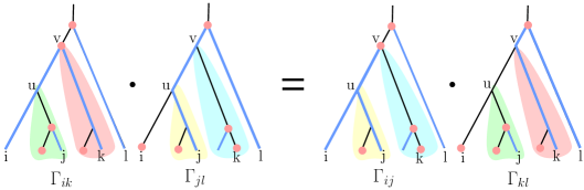
Figure 3. Illustration of the construction for (19) in the proof of Lemma 5.1.

By construction, the power of $\theta_{v}$ coincides on both sides of (19) and so the corresponding terms in (18) will cancel out. What is left is a sum of weights of trek systems, and hence a sum of products of parameters $\theta_{i}$. ∎

Remark 5.5.

A similar construction, also based on Proposition 5.3, can be used to show that the terms in $p_{ik}p_{jl}s^{2}$ are precisely equal to the terms in $p_{il}p_{jk}s^{2}$. This gives an alternative proof of the equations in (10) and hence of Theorem 1.2.

We now prove the semialgebraic characterization of Brownian motion tree models.

Proof of Theorem 2.6.

We first claim that it suffices to show the result for binary trees. Indeed, just like in (12), non-binary models are intersections of binary models:

(20) $$\mathcal{L}_{T,\geq}^{-1}\quad=\quad\bigcap_{\tilde{U}\in[\tilde{T}]}\mathcal{L}_{U,\geq}^{-1}$$

Moreover, the inequalities for $T$ in (10) are those for binary $U$, as $\tilde{U}$ runs over $[\tilde{T}]$. Hence we can assume that $T$ is binary. Suppose that $K\in\mathcal{L}_{T,\geq}^{-1}$. By [VN93, Theorem 2.2], we know that $K$ is positive definite and $p_{ij}\geq 0$ for all $0\leq i<j\leq n$. Theorem 1.2 shows that $K$ satisfies the equalities in (10). In Lemma 5.1 we saw that the inequalities in (10) hold for $K$. Hence all constraints in (10) are satisfied for $K$.

For the converse, let $K\in\mathbb{S}^{n}_{+}$ satisfy (10). By Theorem 1.2, the equations in (10) imply that $K\in\mathcal{L}_{T}^{-1}$. Since $K$ is invertible we can define $\Sigma=K^{-1}$ and $\Sigma=\Sigma_{\theta}$ for some real vector $\theta$. To complete the proof, we must show that $\theta$ is nonnegative.

For any subset $A\subset\{1,\ldots,n\}$ denote by $T_{A}$ the tree whose vertices $V_{A}$ are ${\rm lca}(i,j)$ for $i,j\in A$. There is a directed edge $u\to v$ in $T_{A}$ if there is a directed path from $u$ to $v$ in $T$ containing no other vertices of $T_{A}$. As before, we attach an extra vertex $0$ to the root. Moreover, if $T$ has edge weights $\theta_{v}$ for $v\in V$ then $T_{A}$ has edge weights

(21) $$\tilde{\theta}_{v}\;=\;\sum_{u<w\leq v}\theta_{w}\qquad\mbox{ for }u\to v\,\,\mbox{ in }T_{A}.$$

For example, if $T$ is the tree in Figure 1 and $A=\{1,2,3\}$ then $T_{A}$ has vertices $V_{A}=\{1,2,3,5,7\}$ and edges $0{\to}7$, $7{\to}3$, $7{\to}5$, $5{\to}1$, $5{\to}2$. The weights of $T_{A}$ are

$$\tilde{\theta}_{1}=\theta_{1},\quad\tilde{\theta}_{2}=\theta_{2},\quad\tilde{\theta}_{3}=\theta_{3}+\theta_{6},\quad\tilde{\theta}_{5}=\theta_{5},\quad\tilde{\theta}_{7}=\theta_{7}.$$

If $\Sigma$ lies in the subspace $\mathcal{L}_{T}$ of $\mathbb{S}^{n}$, with weights $\theta_{w}\in\mathbb{R}$, then its principal submatrix $\Sigma_{A,A}$ lies in the subspace $\mathcal{L}_{T_{A}}$ of $\mathbb{S}^{|A|}$. Indeed, the entries of $\Sigma_{A,A}$ are

$$\sigma_{ij}\;\,=\,\sum_{v\leq{\rm lca}(i,j)}\theta_{v}\quad\;=\sum_{v\in V_{A}:\;v\leq{\rm lca}(i,j)}\!\!\!\tilde{\theta}_{v}.$$

In other words, $\Sigma_{A,A}$ can be written as a matrix in $\mathcal{L}_{T_{A}}$ with edge weights (21).

As the main step in the proof, we will now show that the constraints in (10) behave nicely with respect to marginalization to the subtree induced on the subset $A$. Namely, we claim that $\tilde{K}=(\Sigma_{A,A})^{-1}$ is a diagonally dominant M-matrix satisfying

(22) $$\tilde{p}_{ik}\tilde{p}_{jl}\;=\;\tilde{p}_{il}\tilde{p}_{jk}\;\leq\;\tilde{p}_{ij}\tilde{p}_{kl}$$

for all $i,j,k,l\in A\cup\{0\}$ such that the paths $\overline{ij}$, $\overline{kl}$ in $\tilde{T}_{A}$ have no edges in common.

The fact that $\tilde{K}=(\Sigma_{A,A})^{-1}$ is a diagonally dominant M-matrix follows directly from [CM79, Corollary 2]. To show the second part of the claim, we shall assume $|A|=n-1$, say $A=\{1,\ldots,n-1\}$. The general case will then follow by induction.

If $K=\Sigma^{-1}$ then $\tilde{K}=K_{A,A}-\frac{1}{\kappa_{nn}}K_{A,n}K_{n,A}$, by taking the Schur complement. Hence

$$\begin{matrix}\tilde{p}_{ij}&=&p_{ij}+\frac{1}{\kappa_{nn}}p_{in}p_{jn}&&&\hbox{for all $i,j\in A$},\vskip 3.0pt plus 1.0pt minus 1.0pt\\ \tilde{p}_{0i}&=&p_{0i}+p_{in}-\frac{1}{\kappa_{nn}}p_{in}\sum_{j=1}^{n-1}p_{jn}&=&p_{0i}+\frac{1}{\kappa_{nn}}p_{0n}p_{in}&\hbox{for $i\in A$}.\end{matrix}$$

For the quartet $ij|kl$ we conclude

$$\begin{matrix}\tilde{p}_{ik}\tilde{p}_{jl}&=&p_{ik}p_{jl}+\frac{1}{\kappa_{nn}}p_{ik}p_{jn}p_{ln}+\frac{1}{\kappa_{nn}}p_{in}p_{kn}p_{jl}+\frac{1}{\kappa_{nn}^{2}}p_{in}p_{jn}p_{kn}p_{ln},\vskip 3.0pt plus 1.0pt minus 1.0pt\\ \tilde{p}_{il}\tilde{p}_{jk}&=&p_{il}p_{jk}+\frac{1}{\kappa_{nn}}p_{il}p_{jn}p_{kn}+\frac{1}{\kappa_{nn}}p_{in}p_{ln}p_{jk}+\frac{1}{\kappa_{nn}^{2}}p_{in}p_{jn}p_{kn}p_{ln}.\end{matrix}$$

By assumption, $p_{ik}p_{jl}=p_{il}p_{jk}$. We must show that the following expression is zero:

(23) $$\tilde{p}_{ik}\tilde{p}_{jl}-\tilde{p}_{il}\tilde{p}_{jk}\;\;=\;\;\frac{1}{\kappa_{nn}}\left(p_{ik}p_{jn}p_{ln}+p_{in}p_{kn}p_{jl}-p_{il}p_{jn}p_{kn}-p_{in}p_{ln}p_{jk}\right).$$

Figure 4 shows the five cases of where $n$ can be located in $\tilde{T}$. First rewrite (23) as

$$\begin{matrix}\frac{1}{\kappa_{nn}}\left(p_{jn}(p_{ik}p_{ln}-p_{il}p_{kn})+p_{in}(p_{kn}p_{jl}-p_{ln}p_{jk})\right).\end{matrix}$$

In the three cases in the top row of Figure 4, the paths $\overline{in}$ and $\overline{jn}$ do not intersect with the path $\overline{kl}$. This implies, by our assumption on $K$, that $p_{ik}p_{ln}-p_{il}p_{kn}=p_{kn}p_{jl}-p_{ln}p_{jk}=0$ and so (23) is zero. For the remaining two cases we write (23) as

$$\begin{matrix}\frac{1}{\kappa_{nn}}\left(p_{ln}(p_{ik}p_{jn}-p_{in}p_{jk})+p_{kn}(p_{in}p_{jl}-p_{il}p_{jn})\right).\end{matrix}$$

Since the path $\overline{ij}$ does not intersect the paths $\overline{kn}$ and $\overline{ln}$, we conclude the identities $\,p_{ik}p_{jn}-p_{in}p_{jk}=p_{in}p_{jl}-p_{il}p_{jn}=0$. This again implies that (23) is zero.

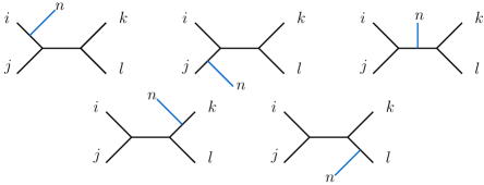
Figure 4. The five cases for adding a leaf $n$ to the quartet $ij|kl$.

It remains to show that $\tilde{p}_{il}\tilde{p}_{jk}\leq\tilde{p}_{ij}\tilde{p}_{kl}$. Similarly as above we obtain

$$\tilde{p}_{il}\tilde{p}_{jk}-\tilde{p}_{ij}\tilde{p}_{kl}\;=\;(p_{il}p_{jk}-p_{ij}p_{kl})+\frac{1}{\kappa_{nn}}\left(p_{il}p_{jn}p_{kn}+p_{in}p_{ln}p_{jk}-p_{ij}p_{kn}p_{ln}-p_{in}p_{jn}p_{kl}\right).$$

By assumption $p_{il}p_{jk}-p_{ij}p_{kl}\leq 0$. We will show that the second term, denoted by $C$, is also nonpositive. Consider the five cases in Figure 4 and write $C$ in two ways:

(24) $$\begin{matrix}C&=&\frac{1}{\kappa_{nn}}\left(p_{kn}(p_{il}p_{jn}-p_{ij}p_{ln})+p_{in}(p_{ln}p_{jk}-p_{jn}p_{kl})\right)\\[5.69046pt] &=&\frac{1}{\kappa_{nn}}\left(p_{jn}(p_{il}p_{kn}-p_{in}p_{kl})+p_{ln}(p_{in}p_{jk}-p_{ij}p_{kn})\right).\end{matrix}$$

The following table shows the signs of the four relevant terms according to each case:

	1	2	3	4	5
$p_{il}p_{jn}-p_{ij}p_{ln}$	$0$	$+$	$-$	$-$	$-$
$p_{ln}p_{jk}-p_{jn}p_{kl}$	$-$	$-$	$-$	$0$	$+$

	1	2	3	4	5
$p_{il}p_{kn}-p_{in}p_{kl}$	$-$	$-$	$-$	$+$	$0$
$p_{in}p_{jk}-p_{ij}p_{kn}$	$+$	$0$	$-$	$-$	$-$

Writing $C$ as in the first line of (24) implies nonpositivity in cases 1, 3, and 4. For the two remaining cases we use the second line. We conclude that $C\leq 0$ in all five cases. This completes the proof of the claim  (22).

We now finally show that $\theta_{v}\geq 0$ for every edge $u\to v$ in $T$. Fix $A=\{i,j,k\}\subset\{1,\ldots,n\}$ such that $v={\rm lca}(i,j)$ and $k\in{\rm de}(u)\backslash{\rm de}(v)$ so that ${\rm lca}(i,k)={\rm lca}(j,k)=u$. Here we allow for $i=j$ if $v$ is a leaf and no $k$ if $u=0$. These two cases with $|A|=2$ will be considered separately; for now assume $|A|=3$. Consider the induced tree $T_{A}$. By construction, $u\to v$ is an edge of $T_{A}$. By the claim above, $\Sigma_{A,A}\in\mathcal{L}_{T_{A}}$ is parameterized by $\tilde{\theta}$ with $\tilde{\theta}_{v}=\theta_{v}$. Example 5.2 ensures that $\tilde{\theta}$ is a nonnegative vector; in particular $\tilde{\theta}_{v}=\theta_{v}\geq 0$. The case when $v$ is a leaf or when $u=0$ are similar, but here $|A|=2$, so we use the case $n=2$. This shows that, for any matrix $\Sigma$ satisfying the constraints (10), it follows that $\Sigma^{-1}\in\mathcal{L}_{T,\geq}^{-1}$. This completes the proof. ∎

Theorem 2.6 offers a geometric understanding of maximum likelihood estimation for Brownian motion tree models. Given any sample covariance matrix $S$, the estimated concentration matrix $\hat{K}$ satisfies (10). If all inequalities are strict for the estimates $\hat{p}_{ij}$ then we are in the situation of Section 4. Otherwise, we have $\hat{p}_{ij}=0$ or $\hat{p}_{il}\hat{p}_{jk}=\hat{p}_{ij}\hat{p}_{kl}$ for some choice of indices in (10). This corresponds to $\hat{\Sigma}={\hat{K}}^{-1}$ lying on a proper face of the simplicial cone $\mathcal{L}_{T,\geq}$. It is interesting to record these faces.

Example 5.6 ($n=4$).

Fix the tree $T$ in Figure 1. The following experiment was performed $1000$ times. We fix the parameters $\,\theta_{1}=\cdots=\theta_{7}=1\,$ and the sample sizes $N=5$ and $N=20$. We sample $N$ vectors from $\mathbb{R}^{4}$ using the Gaussian distribution $\Sigma_{\theta}$ and we record the resulting sample covariance matrix $S$. In each case we compute the MLE $\hat{\Sigma}$ using the standard function for constrained optimization in the statistical software R. For every iteration we check the KKT conditions to see whether the convergence criterion was met. In the affirmative case we identify the face of the $7$-dimensional cone $\mathcal{L}_{T,\geq}$ that contains $\hat{\Sigma}$ in its relative interior. The following table shows the empirical distribution of the codimension of the faces that were found:

codim	0	1	2	3	>3
$N=20$	816	183	1	0	0
$N=5$	487	374	119	20	0

The numbers in the last column are zero because the faces of dimension less than four have empty intersection with the cone of positive definite matrices. In the majority of the experiments, the MLE occurred in the interior of $\mathcal{L}_{T,\geq}$. In this case, the analysis in Example 4.4 applies: the MLE $\hat{\Sigma}$ has algebraic degree five over the data $S$. ∎

Every face of the simplicial cone $\mathcal{L}_{T,\geq}$ has the form $\mathcal{L}_{T^{\prime},\geq}$, where $T^{\prime}$ is obtained from $T$ by contracting some edges. If MLE $\hat{\Sigma}$ lies on that face, then the algebraic complexity of the MLE is governed by the ML degree for $T^{\prime}$. This underscores the relevance of results like Proposition 4.6, even if the tree $T$ of interest is not binary.

Theorem 2.6 implies that the facial structure of the simplicial cone $\mathcal{L}_{T,\geq}$ translates into a stratification of the boundary of $\mathcal{L}_{T,\geq}^{-1}$. This enables a detailed geometric analysis of the MLE across all strata. We shall pursue this in a forthcoming paper.

References

- [And70] Theodore W. Anderson. Estimation of covariance matrices which are linear combinations or whose inverses are linear combinations of given matrices. In I. M. Mahalanobis, P. C. Rao, C. R. Bose, R.C. Chakravarti and K. J. C. Smith, editors, Essays in Probability and Statistics, pages 1–24. Univ. of North Carolina Press, Chapel Hill, 1970.
- [BFF18] Lara Bossinger, Xin Fang, Ghislain Fourier, Milena Hering and Martina Lanini. Toric degenerations of Gr(2,n) and Gr(3,6) via plabic graphs. Annals of Combinatorics 22(3): 491–512, 2018.
- [Bun71] Peter Buneman. The recovery of trees from measures of dissimilarity. In F. Hodson et al., editor, Mathematics in the Archaeological and Historical Sciences, pages 387–395. Edinburgh University Press, 1971.
- [CM79] David Carlson and Thomas L Markham. Schur complements of diagonally dominant matrices. Czechoslovak Mathematical Journal, 29(2):246–251, 1979.
- [DMSM14] Claude Dellacherie, Servet Martinez, and Jaime San Martin. Inverse M-matrices and ultrametric matrices, volume 2118. Springer, 2014.
- [DST13] Jan Draisma, Seth Sullivant, and Kelli Talaska. Positivity for Gaussian graphical models. Advances in Applied Mathematics, 50(5):661–674, 2013.
- [Fel73] Joseph Felsenstein. Maximum-likelihood estimation of evolutionary trees from continuous characters. American Journal of Human Genetics, 25(5):471–492, September 1973.
- [M2] Daniel Grayson and Michael Stillman. Macaulay2, a software system for research in algebraic geometry. Available at http://www.math.uiuc.edu/Macaulay2/.
- [KM19] Kiumars Kaveh and Christopher Manon. Khovanskii bases, higher rank valuations and tropical geometry. SIAM Journal on Applied Algebra and Geometry, 2019.
- [MS15] Diane Maclagan and Bernd Sturmfels. Introduction to Tropical Geometry, volume 161 of Graduate Studies in Mathematics. American Mathematical Society, Providence, 2015.
- [MSUZ16] Mateusz Michałek, Bernd Sturmfels, Caroline Uhler, and Piotr Zwiernik. Exponential varieties. Proceedings of the London Mathematical Society (3), 112(1):27–56, 2016.
- [MS04] Vincent Moulton and Mike Steel. Peeling phylogenetic ’oranges’, Advances in Applied Mathematics, 33(4): 710-727, 2004.
- [STD10] Seth Sullivant, Kelli Talaska, and Jan Draisma. Trek separation for Gaussian graphical models. Annals of Statistics, 38(3):1665–1685, 2010.
- [VN93] Richard S. Varga and Reinhard Nabben. On symmetric ultrametric matrices. Numerical Linear Algebra (eds L. Reichel et al.), de Gruyter, New York, pp. 193–199, 1993.
- [ZUR17] Piotr Zwiernik, Caroline Uhler, and Donald Richards. Maximum likelihood estimation for linear Gaussian covariance models. Journal of the Royal Statistical Society: Series B (Statistical Methodology), 79(4):1269–1292, 2017.